Stratification Breakdown by Fall Cold Front Winds over the Louisiana Shelf in the Northern Gulf of Mexico: A Numerical Experiment

Abstract

Cold fronts are meteorological phenomena that impact the northern Gulf of Mexico, mostly between the fall and spring seasons. On average, they pass the region every 3–7 days, with a duration ranging between 24 and 74 h. In the present study, a high-resolution FVCOM model with an unstructured mesh was used to simulate the effect of the fall cold front winds on water column mixing over the Louisiana shelf, which is often stratified in the summer, leading to hypoxia. Numerical experiments were conducted for October 2009, a period with five consecutive cold front events. Winds from an offshore station forced the model, while climatological temperature/salinity profiles prepared by NOAA for September were used for model initialization. The model performance was evaluated by comparing it with the surface current measurements at two offshore stations, and the results showed a good agreement between the model results and observations. Shelf mixing and stratification were investigated through examining the simulated sea surface temperature as well as the longitudinal and cross-shelf vertical sections. Simulation results showed a significant effect on shelf mixing, with the mixed layer depth increasing from the initial values of 5 m to 25 m at the end of simulation at different parts of the shelf, with maximum mixed layer depths corresponding to the peak of cold fronts. The buoyancy frequency, Richardson number, and the average potential energy demand (APED) for mixing the water column were used to quantify the stratification at two selected locations over the shelf. Results showed that all these parameters almost continuously decreased due to mixing induced by cold front wind events during this time. At the station off the Terrebonne Bay with a water depth of 20 m, the water column became fully mixed after three of the cold front events, with Richardson numbers smaller than 0.25 and approaching zero. This continued mixing trend was also proven by obtaining a decreasing trend of APED from 100 to 5 kg/m.s² with several close to zero energy demand values.

1. Introduction

The stratification over the Louisiana continental shelf in the northern Gulf of Mexico has a seasonal variation [1]. Starting from the late spring to the end of summer, due to weak wind stress and increasing solar radiation during this time of the year, the water column significantly stratifies, with the Richardson number being much larger than the mixing threshold of 0.25 [2]. The other significant contributor to increasing the stratification in this region during the summertime is the discharge of fresh water from the Mississippi River to the shelf, with its peak during January–June [3,4,5], significantly increasing the water column buoyancy.

This strong stratification substantially influences the continental shelf hydrodynamics and biogeochemical processes [6,7,8]. With the reduced surface wind stress, water column stratification can influence the pattern of shelf currents at the surface and bottom [6,9,10]. Summertime stratification is the main physical factor contributing to the seasonal hypoxia in the northern Gulf of Mexico extending west of the Bird’s Foot Delta over the Texas–Louisiana Shelf [11,12,13,14]. During this time, the strong stratification across the water column significantly limits the reaeration of the water beneath the stratified surface layer, especially the bottom water. At the same time, the enhanced biogeochemical activities across the water column due to high water temperature and the large load of nutrients from the Mississippi River substantially increase the oxygen consumption. This causes the water oxygen concentration, especially at the bottom, to decline to less than 2 mg/L, reaching hypoxic conditions [12]. This shelf-wide lack of oxygen in the bottom water during the summer continues until fall. It may be occasionally broken down by tropical cyclones that pass over the shelf from June to November [15,16]. For instance, during Hurricane Katrina, the stratification was broken down for a short time period before and after the final landfall of the hurricane within a region of 50 km of the track. However, these extreme atmospheric events affect the shelf within a short period, from several hours to days. Their mixing effect is mostly local, with significant mixing only in the vicinity of the track [16]. Therefore, their impact on mixing is ephemeral, and the stratification starts to rebuild right after the storm wind is dissipated. In the case of Hurricane Katrina over the shelf, the stratification started to rebound 6–12 h after the landfall, even for regions in the proximity of the track.

Continuous wind forcing can cause sustained mixing across the water column. An example of this is monsoon winds in the northern Arabian Sea and the Gulf of Oman that persist for three to four months in the summer and cause significant mixing and coastal upwelling in these regions [17]. Unlike tropical cyclones in the northern Gulf of Mexico, cold fronts occur frequently and more regularly in non-summer seasons. Together with the increased wind stress, cold fronts also bring cold air from the north and reduce the ocean temperature, thereby contributing even more to the destruction of stratification established in the summer. This situation can be sustained in the region during the fall and spring when cold fronts are frequent [18,19,20,21,22]. Their outbreak period is every 3–7 days, and their duration is 24–74 h, associated with generally northerly winds. A myriad of studies has shown that cold fronts impact various hydrodynamic, biogeochemical, and transport properties of the estuaries, bays and continental shelf (e.g., [23,24]). Feng and Li [23] showed that, during the cold fronts, substantial flushing of the coastal bays takes place toward the inner shelf. A numerical model of the shelf currents by Allahdadi et al. [24] demonstrated that cold fronts contribute discharge of a high load of sediments from the Atchafalaya–Vermillion Bay system to the Louisiana shelf during the high stage of the Atchafalaya River. This sediment load is then transported westward under the upcoast shelf currents and contributes to the formation of Chenier plains along the west coast of Louisiana.

One less-studied effect of severe cold fronts on the Louisiana shelf is their role in mixing the water column and breaking down the summertime strong stratification over the shelf that maintains the hypoxia. Although the weakening of the solar radiation during the fall can also contribute to reducing the stratification, the intense mixing caused by strong wind shear stress can also be a significant contributor. As shown by Allahdadi et al. [2], there is a direct relationship between the seasonally variable wind stress and the horizontal shear observed in the vertical current profiles at different locations over the shelf. They concluded that, during the low wind stress season of summer, the current shear is one order of magnitude smaller than the high wind stress season of fall. This higher current shear during the fall can be a major driving force for weakening and eventually breaking down of the stratification sustained during the summer. The study of Allahdadi et al. 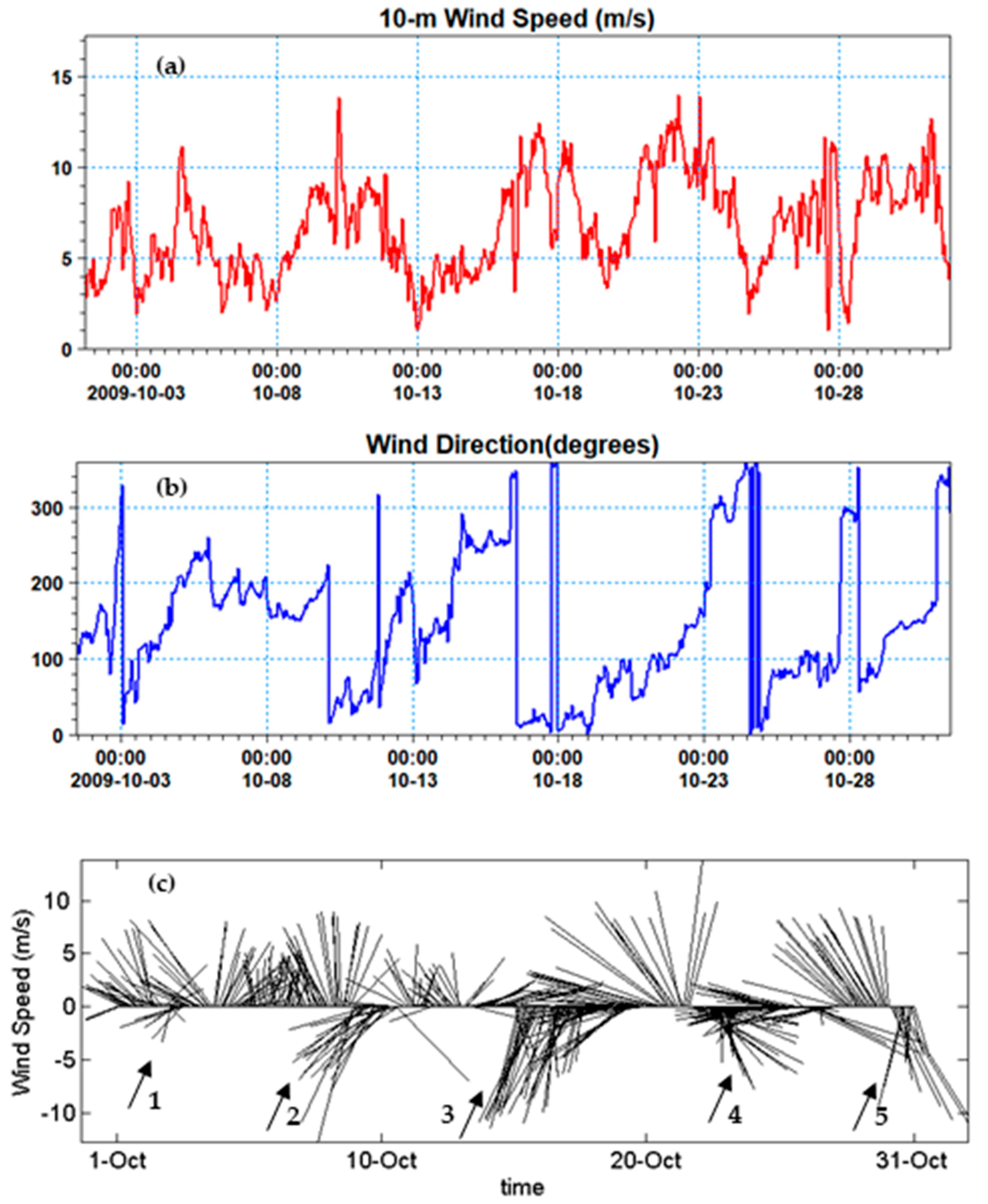[2] is one of the few studies investigating the mixing of the Louisiana shelf during different seasons, although only current velocity data were used. More studies are needed to address the mechanism and pattern of shelf mixing during the fall season and demonstrate the effect of high wind stress as a result of consecutive cold front events on shelf mixing. This will help the understanding of the physical mechanisms contributing to the seasonal hypoxia in the region and for a better approach to quantify and predict the evolution of seasonal hypoxic events each year. In the present study, numerical experiments using FVCOM were performed to study if/how the cold front wind stress can turn a strong stratification across the water column into a more mixed water column. A one-month continuous simulation forced by only wind stress during October 2009, a month that included five consecutive cold front events, was implemented. No solar radiation input was included in the simulation to focus on the effect of wind stress. The model performance was evaluated using the observed currents from two WAVCIS stations off Barataria and also the Terrebonne/Timalier Bay. The evolution of the stratified water column to a mixed water column over the shelf was investigated using the along- and cross-shelf transects. The stratification/mixing during the simulation period was quantified using the Richardson number, buoyancy (Brunt–Väisälä) frequency, and average potential energy demand (APED).

2. Study Region

The focus of this study is the Louisiana continental shelf in the northern Gulf of Mexico (Figure 1). The shelf is characterized by a rather complicated bathymetry with higher depths of up to 60–70 m right on the west of the Mississippi Bird’s Foot Delta (east side of the shelf) and smaller depths less than 10–15 m off the Atchafalaya Bay on the west side of the shelf (Figure 2a). Approaching the west regions, the shelf slope significantly decreases, which can substantially affect the shelf hydrodynamics and temperature/salinity response to storm events [24]. The coastline on the north of the shelf has a complex geometry. It includes several bay–estuarine systems like Barataria Bay, Terrebonne/Timbalier Bay, and Atchafalaya Bay. During cold fronts, flushing [23] from these bays to the shelf area highly contributes to the hydrodynamics and biogeochemical processes on the shelf.

3. Numerical Model Specification

3.1. Model

In this study, the finite volume community ocean model (FVCOM) is used for simulating the effect of consecutive cold fronts in fall on the shelf mixing. FVCOM is a circulation/heat/salt/pollutant transport model that solves the three-dimensional (3D) governing equations (momentum balance, continuity, energy conservation, and mass conservation) on an unstructured triangular mesh using the finite volume method [25]. A hydrostatic pressure balance across the water column is assumed, which is a reasonable assumption due to the negligible vertical acceleration in most practical cases. The momentum equation uses the Boussinesq approximation to resolve the density variations, which is acceptable for most oceanic, coastal, and estuarine waters. Horizontal momentum terms are resolved using the Smagorinsky turbulent closure scheme, while, for vertical eddy viscosity and diffusivity, the Mellor–Yamada level 2.5 turbulence closures are applied. Two parameters associated with the vertical eddy viscosity (background eddy viscosity and the coefficient B for calculating the turbulence energy dissipation) are used for tuning simulated currents, temperature, and salinity. More details on the FVCOM model and its implementation are presented in Appendix A.

3.2. Study Area and Computational Mesh

A modeling area with a circular open boundary extending from Mobile, Alabama, on the east to Sabine Lake, Texas, on the west of the Mississippi Bird’s Foot Delta was used (Figure 2a). The model boundary is extended to the outer shelf to consider the exchange between the inner and outer shelves that affects the shelf temperature and salinity. An unstructured computational mesh generated by triangular elements is used (Figure 2b). This computational mesh, with a coarse resolution of 10 km along the offshore boundary, was refined to about 500 m over the inner shelf. Selection of the computational resolution through examining different meshes and comparing the results (mesh sensitivity analysis) was done thoroughly at the beginning of this study. Sensitivity analysis was done on the mesh resolution. Coastal resolutions from 100 m to 700 m were tried, and it was found that the current pattern and values and temperature/salinity were similar for resolution between 100 and 600 m. Therefore, a coastal resolution of 500 m was used as the optimally computational resolution for the present modeling. The external and internal time steps were assumed to be 6 s and 60 s, respectively, based on CFL criteria.

3.3. Initial Temperature/Salinity Profiles

The stratification status at the beginning of the simulation was defined by introducing the shelf-wide profiles of temperature and salinity. Since the intended simulation period in this study is October 2009, temperature and salinity profiles around 1 October are required. However, there are no such observations available. Hence, climatological data were used as the model initial condition for temperature and salinity. The climatological data represent each month’s average temperature and salinity across the water column and can represent the average stratified conditions established in the summer. In this paper, climatological profiles from the World Ocean Atlas (WOA) database were selected as the initial condition (http://www.nodc.noaa.gov/access/allproducts.html, accessed on 15 March 2023) for the month prior to the simulation (September). The horizontal resolution of this gridded dataset is 0.25 degrees, and temperature and salinity are represented at 57 depths from the surface to a depth of 1500 m at the open boundary. The vertical resolution is 5 m for the upper 100 m, 25 m for the depths 100–500 m, and 50 m for the depths 500–1500 m. Several studies, including those of Koohestani et al. [7] and Pan and Sun [26], showed the proper accuracy of these data as the model’s initial condition during the storm conditions. In the version of FVCOM used in this simulation, the initial conditions should be represented at each computational grid point of the unstructured mesh. Hence, we interpolated the climatological data with 0.25 degree resolution on the computational mesh across the standard vertical levels (consistent with the vertical resolution of climatological data) defined in the model setup. Figure 3 shows a sample of climatological profiles used for September at a location off Terrebonne/Timbalier Bay with a water depth of 250 m.

3.4. Wind Data

The model was forced with the wind measured at the WAVCIS station CSI-6 in October 2009. The measured wind speeds at this station were reduced to the standard level of 10 m above the sea level, and wind speed and direction were uniformly applied to the model. Several former studies, including [1,22], showed that the measured wind at a station over the shelf could result in acceptable hydrodynamics during the cold fronts if uniformly applied to a shelf-wide model. Another study by Chaichitehrani et al. [27] showed that, even for the summer mild storms, the speed and direction of wind over the Louisiana shelf could approximately be considered uniform. Examining the spatially varied wind fields simulated by the Climate System Forecast Reanalysis (CFSR) showed that, during the peak of cold fronts in October 2009, the wind field over the Louisiana shelf was almost uniform (Figure 4). Spatially varied patterns were mostly observed during the frontal passage when the wind direction was changing from southern to northern quadrants. This time period is relatively short, and a constant wind field is an approximation valid for most of the time period on time scales longer than inertial periods.

The measured wind data at CSI-6 showed five consecutive cold front events with different intensities and directions from northwest to northeast (Figure 5b,c). For the three events between 8 and 25 October, wind speeds exceeded 10 m/s and reached 13 m/s for two of them.

3.5. Model Setup

Using the bathymetry and the computational mesh shown in Figure 2, the FVCOM model was setup for the Louisiana shelf. It should be noted that no boundary conditions for hydrodynamics and temperature/salinity were applied along the model’s open boundary, so the model could only consider the effect of wind-induced mixing. For bottom friction, the default value of 0.0025 was used. The simulation included 25 vertical sigma layers to resolve the vertical currents, temperature, and salinity variations appropriately.

3.6. Verification of Hydrodynamics Model

The results from the hydrodynamics model were verified by comparing with the measured surface currents at stations WAVCIS CSI-6 and CSI-9 (Figure 1 for location). Sensitivity tests showed that using a constant value for vertical eddy viscosity resulted in a better match-up with measurement than using turbulent closures. This conclusion is consistent with other Louisiana shelf modeling studies, including [24,28]. The best match-up with measurements was obtained using 0.005 m²/s as the constant vertical eddy viscosity. Since no tidal boundary condition was used in the simulation, the measured currents were de-tided and compared with the simulation results (Figure 6). The differences between the simulated and observed currents at these two WAVCIS stations could partly be attributed to the outer shelf dynamics like the effect of the loop-current eddy variations ([24]) not included in the model open boundary in this study. It could also be partly due to the uniform wind field that has been used in the simulation, especially during the frontal passage time when wind shear exists.

4. Results

4.1. Cold-Front-Induced Surface Circulation

For brevity, in this paper we only present the results for temperature structure when discussing the cold-front-induced mixing over the shelf. Cold front wind direction typically changes from southerly to northerly and the system moves from the northwest to southeast and then to northeast. All these can affect the surface currents, depending on the exact movement of the front and wind direction variation, coastal geometry, and the local shelf bathymetry; the speeds and directions of currents are also variable. The wind time series shown in Figure 5 includes the intermittent (episodic) outbreaking of cold front winds with prefrontal southwesterly to southeasterly winds in between. Hence, the resulting circulation during the 1-month simulation includes both offshore-ward and shore-ward current fields (Figure 7). The cold front no. 2 of October 2009 occurred before 10 October. The wind direction at the peak of the cold front is northeasterly, causing southwestward to westward currents on the shelf. On the outer shelf outside of the Mississippi Bird’s Foot Delta and at the shelf break, larger surface current speeds up to 0.25 m/s result due to the significant increase in water depth (larger than 50 m) and thus the decreasing effect of bottom friction. Due to smaller depths on the western part of the Louisiana shelf (10–20 m) and a wider continental shelf in this region, current directions rotate clockwise and direct toward west. The third cold front (no. 3) of the month occurred between 15 and 19 October with the direction of northeasterly to the north; hence the generated currents are expected to be directed more offshore. The current field for 17 October (Figure 7b) shows that, at the peak of the post cold front, northerly winds are going in the southwesterly to southerly directions on the shelf and nearshore region, while the peak of currents in the nearshore region reaches 0.3 m/s. The current field shown on 22 October (Figure 7c) is related to the pre-frontal phase of the next cold front (cold front no. 4). This phase includes changing wind direction to the southern quadrants that produces currents toward the inner shelf with the general direction of northward. After the passage of cold front no. 4, the wind direction is from the northwest, generating southeasterly shelf currents (Figure 7d). The peak of the wind speed and duration of winds for this event is smaller than events 2 and 3; thereby, smaller current speeds with peak values of 0.2 m/s are generated. It should be noted that the bottom currents (not shown) over the Louisiana shelf are not to the same as the surface current or wind and have different directions (generally opposite) compared with the surface currents since they are controlled by the pressure gradient over the shelf [29].

4.2. Sea Surface Temperature

The initial SST over the shelf, as defined by the climatological temperature profiles (e.g., Figure 3a) is 30–30.5 °C. The water column mixing and shelf circulation (as of Section 4.1) contribute to the evolution of this distribution. Ten days into the simulation (at 12:00 a.m., 10 October), the SST over the offshore shelf region decreases to 29.5–29.8 °C, while, at the coastal regions, the SST still maintains the original values of greater than 30 °C. Higher current speeds over the offshore area as a result of peak post-frontal wind associated with cold front no. 2 (Figure 7a) cause more mixings over these areas that entrain the colder water beneath the water surface to the surface and decrease the SST. A similar pattern and mechanism are observed on 17 October at 12:00 a.m. (Figure 8b), corresponding to the peak of post-frontal wind of cold front no. 3 and the general surface shelf current directed southwestward (Figure 7b). At this time, under the intense circulation and mixing, the SST drops to 29.2 °C. The shelf SST cooling during the post-frontal phase after cold front no. 4 continues, with SST values of 28.5 °C and 29.2 °C for the offshore and mid-shelf regions, respectively. At this point, the surface cooling is due to both the shear entrainment across the water column and the favorable upwelling winds from the southwest (Figure 8c). The high gradient of the SST over the shelf is the result of the dominant wind-induced surface current from the southwest that pushes the water toward the inner shelf. After the peak wind after cold front no. 4 on 27 October, almost the whole shelf reaches SST values less than 29.5 °C, with values less than 30 °C observed everywhere except on the shelf in front of the Atchafalaya Bay (Figure 8d). At this time, the offshore SST drops to 28 °C, about 2 degrees less than the initial SST.

As mentioned earlier, the main objective of this study is examining the effect of cold front wind-induced shelf mixing in breaking down the summertime stratification. Therefore, no solar energy input and no temperature/salinity along the model open boundary were applied for simplicity and for isolating the major effect of wind stress from other factors. Furthermore, due to a lack of field data, the climatological profiles have been used as the initial conditions for temperature and salinity. Therefore, although satellite SST data are available to be compared with simulated SSTs, since the model setup does not include all the temperature forcing, a detailed comparison is not possible.

The SST maps prepared based on the OI-SST product (https://www.remss.com/measurements/sea-surface-temperature/oisst-description/, last access: 28 February 2023) are presented in Figure 9 at times corresponding to Figure 8. As seen, although the observed SST is generally consistent with model simulation, there are some discrepancies as well as anticipated because the model is dependent on climatological initial condition and only forced by wind.

4.3. Shelf-Wide Cross Sections

Time variations of the simulated water temperature across the water column have been investigated across the cross sections along and across the Louisiana shelf. Temperature variations along the shelf have been examined through the longitudinal section AS1 (Figure 1 for location). This section extends from the Mississippi Bird’s Foot Delta on the east to the offshore of Sabine Bank, TX, on the west. The maximum water depth along this section is 65 m on the west of the Mississippi delta, and the minimum is 7 m off the Terrebonne/Timbalier Bay (Figure 10). Water depth on the west of this location shows a relatively shallow shelf with an approximate depth around 20 m. Water temperature variation along this section and across the water column shows a continuous temperature redistribution across the depth, causing more mixing and increasing the mixing depth along the shelf (Figure 10a–f). At 12:00 a.m. on 1 October, the initial temperature profile along the shelf is specified based on climatological data (Figure 10a). The initial shelf-wide temperature profile shows horizontal contour lines corresponding to a strong stratification at the beginning of the simulation. As the wind is applied to the model, shelf-wide temperature distribution across the water column changes, and temperature contours become more inclined and, in some cases, become completely vertical, which is a sign of complete mixing across the water column. On 10 October, after the first cold front affected the region, on the western part of the shelf, especially off the Atchafalaya Bay, the horizontal patterns of the temperature contours are disturbed, and the mixing depth increases from the initial value of 12 m to 16 m. On the eastern part of the Mississippi Bight, the isotherms slope toward the delta under the effect of shelf hydrodynamics and mixing forces (Figure 10b). It should be noted that, over the western shelf, the increase in mixing depth is associated with an increase in water temperature, resulting from the advection of warm water from the offshore area at lower depths by the reversed bottom currents. As stated by Allahdadi et al. [16] for the mixing effect of Hurricane Katrina over the Louisiana shelf, baroclinic instability, which is related to the horizontal gradient of buoyancy, is one of the important re-stratification mechanisms after a storm. Furthermore, lateral gradients of water density itself could cause re-stratification due to gravitational circulation. Both these mechanisms are partly controlled by horizontal (lateral) advection. The intermittent effect of the cold fronts causes almost fully mixed regions for the relatively shallow shelves on the east and west of the shoal off the Barataria Bay, where the water depth is smaller than 30 m (Figure 10e). Even in the deeper regions of the Mississippi Bight, the 30 m upper water column is fully or partially mixed. The average water temperature across the section during the one-month simulation shows a similar trend (Figure 10f). It shows that, over the shallow shelf on the west of the section, the temperature mixing depth increases from 12 m at the beginning of the simulation to 15 m on average at the end of the one-month simulation. In contrast, the deeper shelf on the east of the section, on average, shows a partially mixed water column for the upper 20 m.

Simulated temperature variations across the water column have also been examined along the cross-shelf transect CS A (Figure 1 for location). This transect is located between the Terrebonne/Timbalier and Atchafalaya Bays and extends from the shoreline to a water depth of 65 m across the shelf. Corresponding to the times for which hydrodynamics and shelf-wide temperatures were examined (Figure 7, Figure 8 and Figure 10), cross-shelf temperature variation is also presented (Figure 11). The shelf initial stratification (Figure 11a) shows a 12 m upper mixed layer with the temperature varying from 30 °C at the surface to 22 °C at 60 m depth. Right after the second cold front with southwesterly surface currents, the lower temperature waters in the deeper parts of the water column are mixed with the warmer surface water, especially in the deeper parts of the section (Figure 11b). After the passage of the third cold front (on 17 October), the mixing across the upper 20 m of the water column increases, and the mixing depth in the offshore region increases up to 18 m with a smaller temperature than the initial (28.5 °C vs. 30.0 °C). However, during the pre-frontal phase of the next cold front, the generally northward currents disrupt the mixing produced by the post cold front’s southward currents; thereby, the temperature distribution across the cross-section is similar to 10 October (Figure 11d). Shelf mixing reaches its maximum after the fourth cold front on 22 October, which is associated with northeasterly winds and generated southeasterly surface currents (Figure 11e). At this time, the upper water column up to 20 m depth is mixed for the entire section, with different mixed layer temperatures at offshore, mid-shelf, and coastal regions. Although the one-month average temperature across the section does not show a distinct upper mixed layer, as seen on 22 October, it clearly indicates that the section is in the process of mixing with the temperature isobars inclined offshore-ward, a sign that colder deep water is on the verge of mixing with surface water (Figure 11f).

5. Quantifying Shelf Mixing

In the previous section, the effect of cold front winds on the continuous mixing of the Louisiana shelf was demonstrated qualitatively by examining simulated SST and water column temperature for along-shelf and cross-shelf sections. The gradient Richardson number and buoyancy frequency are used to quantify the shelf mixing or stratification. The Richardson number is calculated as the ratio of buoyancy forces to the shear forces across the water column [30]:

$$R_i=\frac{N^2}{{\left(\frac{\partial u}{\partial z}\right)}^2+{(\frac{\partial v}{\partial z})}^2}$$

(1)

$$N^2=-\frac{g}{{\rho }_0}\frac{\partial \rho }{\partial z}$$

(2)

In the above equations, u and v are horizontal velocity components. Variations of current components in the vertical (z) direction cause vertical mixing. $\rho$ is water density calculated using water temperature and salinity, g is the acceleration of gravity (m/s²), and $N^2$ is buoyancy (Brunt–Väisälä) frequency. The strength of stratification at each depth is indicated by the Richardson number. A Richardson number larger than 1 corresponds to the dominancy of buoyancy forces over shear forces. Hence stratification is stable, and the water column is considered stratified. When the Richardson number is smaller than 0.25, shear and turbulence forces dominate, thereby making the water column unstable, and the water column is mixed [30,31,32].

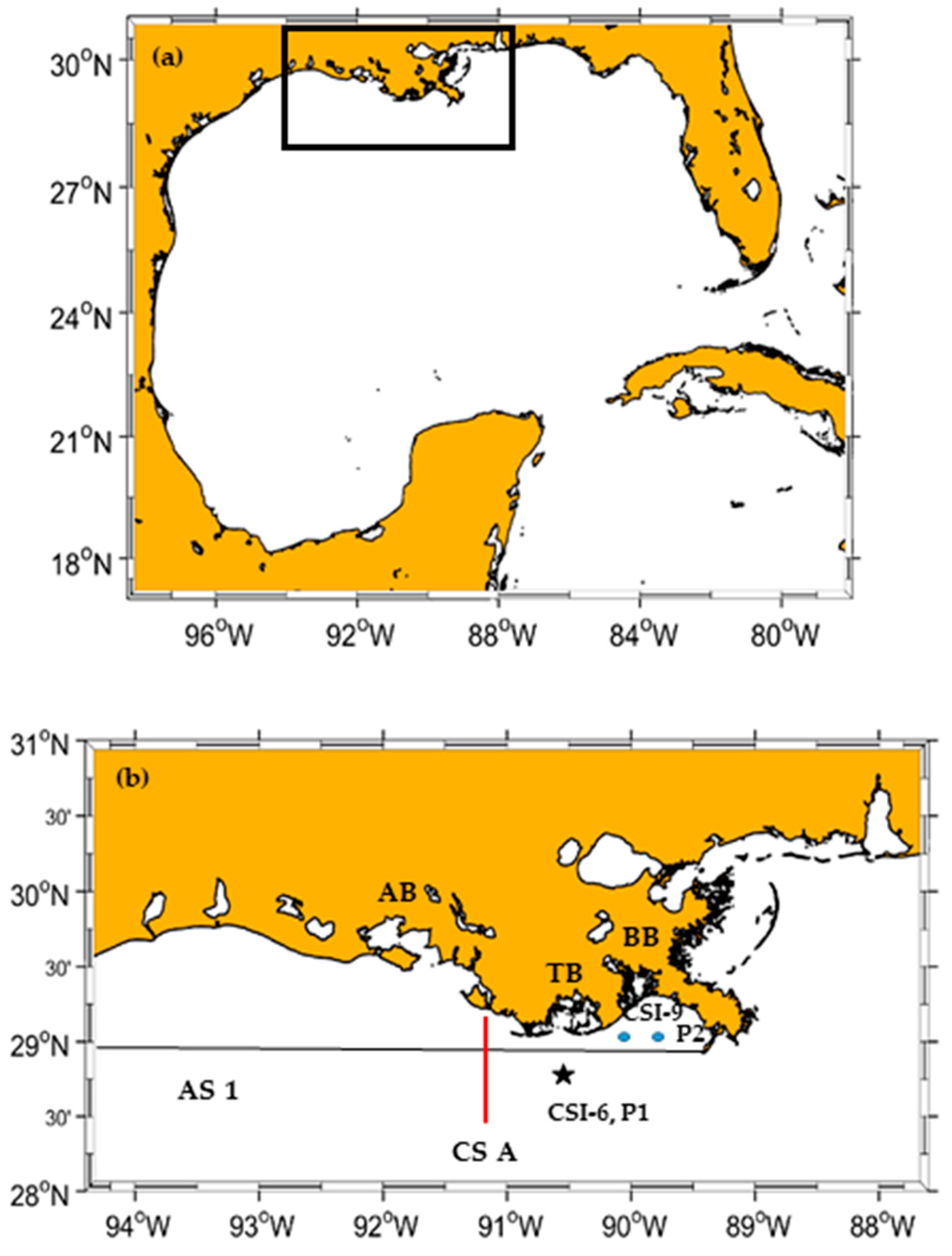
P1 and P2 stations on the shelf were selected for quantifying their mixing/stratification properties during the one-month simulation period (Figure 1 for locations). Station P1 corresponds to the same location as WAVCIS station CSI-6 located off Terrebonne/Timbalier Bay, where the water depth is 20 m. Station P2 is located northeast of station P1, off the Barataria Bay within the Mississippi Bight, with a water depth of ~30 m. 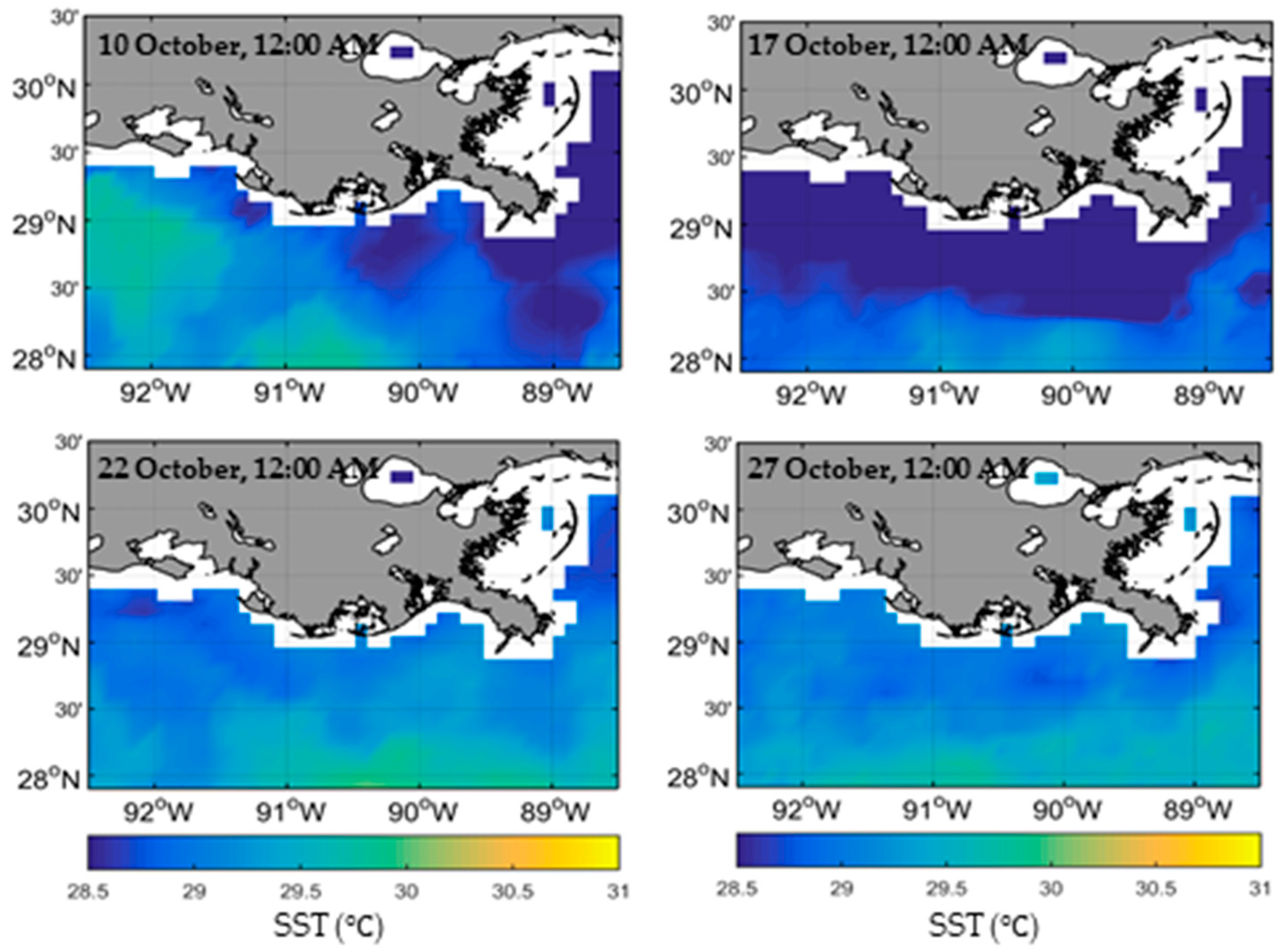Time series of the simulated SST and water temperature across water depth are shown in Figure 12. At both stations, SST continuously decreases during October 2009 due to mixing between the warmer surface water and the colder deep water. It should be noted that here the whole SST reduction is attributed to the wind-induced mixing since no surface heat flux or buoyancy flux were included in this numerical experiment. In Station P1, the SST decreases from the initial value of 31 °C to 29.8 °C, while, at station P2, a smaller value of SST (28.7 °C) results at the end of the simulation. This could be due to the larger depth of station P2 that facilitates mixing colder deep water with the surface warm water at this station. Time series of water temperature across water depth at each station (Figure 12 lower panels) show the time evolution of mixing at these locations. The initially warmer (30.7 °C) upper stratified layer at station P1 (Figure 12, lower left panel) evolves to an almost mixed water column after 10 October with a lower temperature (30.2 °C). Depending on the time of cold air outbreaks, intermittent fully mixed water columns are observed. At the end of the simulation on 31 October, the water column is again fully mixed with the lowest temperature during the simulation (29.7 °C). The upper layer stratification at station P2 is more persistent than that of station P1, and it takes until 20 October for this layer to fully disappear due to mixing. This is due to the more active hydrodynamics at station P1, which is further offshore relative to station P2 (Figure 7) and thereby is exposed to larger mixing forces. Furthermore, the smaller water depth at station P1 can result in larger current speeds. The initial 5 m mixing depth at station P2 increases to 15 m at the end of October when the mixed layer temperature is 29 °C.

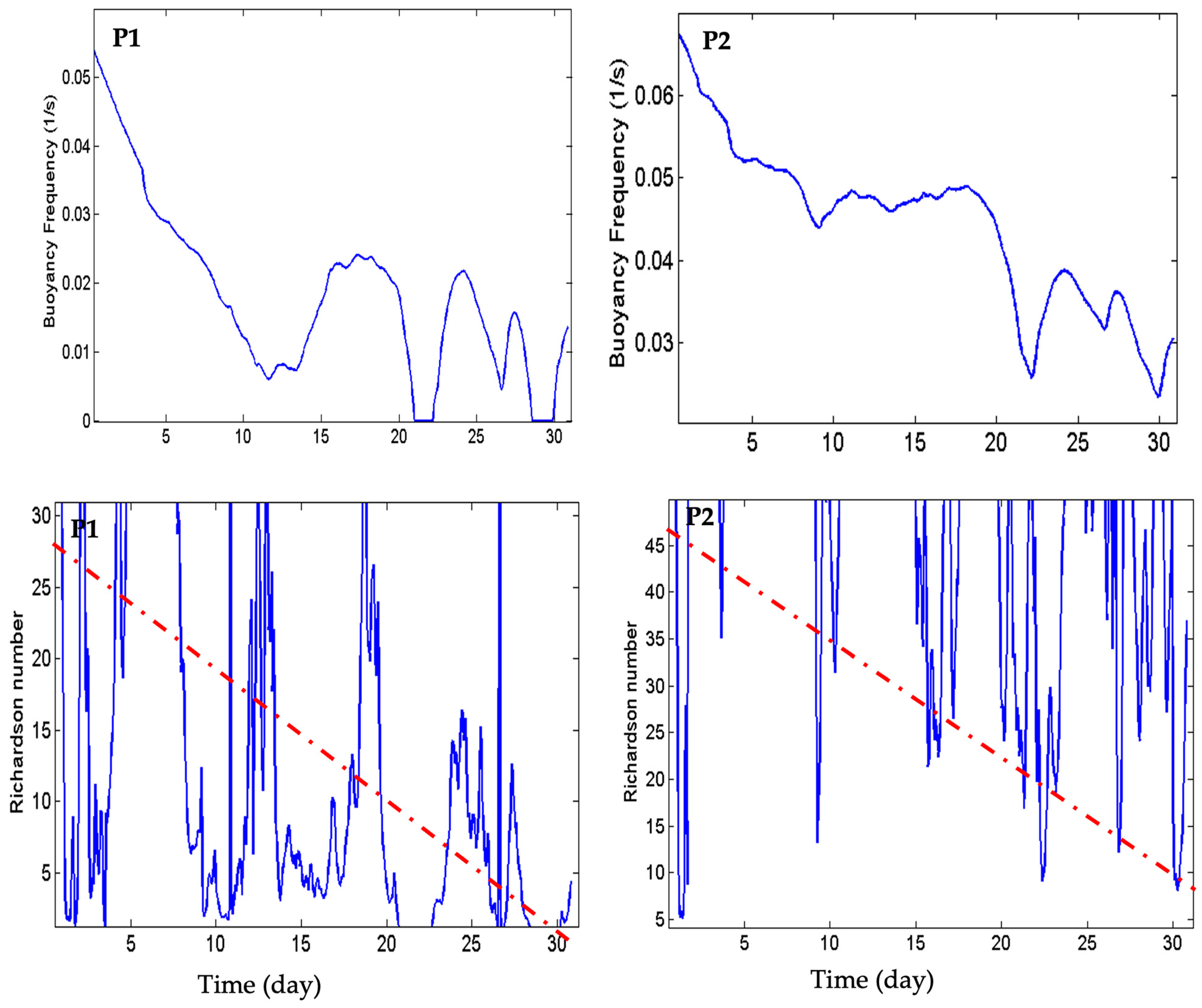
SST and water temperature at both P1 and P2 show a consistent decrease with increases in the mixing depth. Time series of the buoyancy frequency and Richardson number at both stations (Equations (1) and (2)) show similar consistent increases in mixing (Figure 13). Both quantities were calculated at the stations’ mid-depth. Selecting the mid-depth is due to the specific structure of horizontal current across the water depth over the inner Louisiana shelf. Several studies have shown that in this region during different conditions, including cold front, fair-weather conditions and hurricanes, the cross-shelf current follows a two-layer baroclinic system with different and sometimes opposite current directions ([28,29,33]). The change of current direction takes place approximately in the vicinity of the mid-depth; hence the maximum current-induced shear can be observed at the mid-depth. Therefore, the u and v components of current, along with simulated temperature and salinity at the surface and mid-depth, were used in calculations. The general declining trend of the buoyancy frequency at both stations indicates the weakening of stratification strength through time. The buoyancy frequency decreases to a smaller value at P1 compared with that of P2 (0.01 and 0.03/s, respectively), which is consistent with the more mixed water column at station P1, as illustrated in Figure 12.

The calculated mid-depth Richardson numbers also have a declining trend at both stations (Figure 13, lower panels). At the beginning of the simulation and before the intense cold front winds produce relatively large current speeds over the shelf, the very stable stratification at both stations result in very large Richardson numbers (>30–45). The cold-front-event-associated winds produce the shelf currents, contributing to substantial mixings, as indicated by a significant decrease in the Richardson number. At station P1, the Richardson number decreases from about one after the second cold front on 10 October to less than 0.25 (fully mixed water column) on 20 October, before the fourth cold front. Another fully mixed case is observed after the fourth cold front on 27 October. During the pre-frontal time (southeasterly to southwesterly winds) that are dominant between the cold front events, the Richardson number increases to large numbers (strong stratification). However, the general trend of the Richardson number for the whole simulation month (the dashed red line) is to decrease. The decreasing trend of the Richardson number and episodic decreases during and after cold front events is similar at station P2. However, much higher Richardson numbers show a more stable stratification at station P2.

The intensity and duration of the fronts as well as the pre-storm stratification condition contribute to recovering time after each storm. Time series of the shelf mixing/stratification, Richardson number and buoyancy frequency (Figure 12 and Figure 13) can be good manifestations of these effects. Based on these figures and noting that the peak of cold fronts no. 2–5 occurs on 10, 17, 22, and 27 October, respectively, we see that the water column at both P1 and P2 experiences more intense mixings associated with smaller Richardson numbers and buoyancy frequencies compared with the times before the cold fronts. It is also seen that right after cold fronts no. 4 and 5 (after 22 and 27 October) the water column became fully mixed at P1 and more mixed at P2 compared with other events. This more intense mixing after cold fronts no. 4 and 5 could likely be due to the shorter recovering time b, especially the effect of recovering time between each of these and the previous cold front event (7 days between no. 2 and no. 3, 5 days between no. 3 and 5, and 5 days between no. 4 and 5).

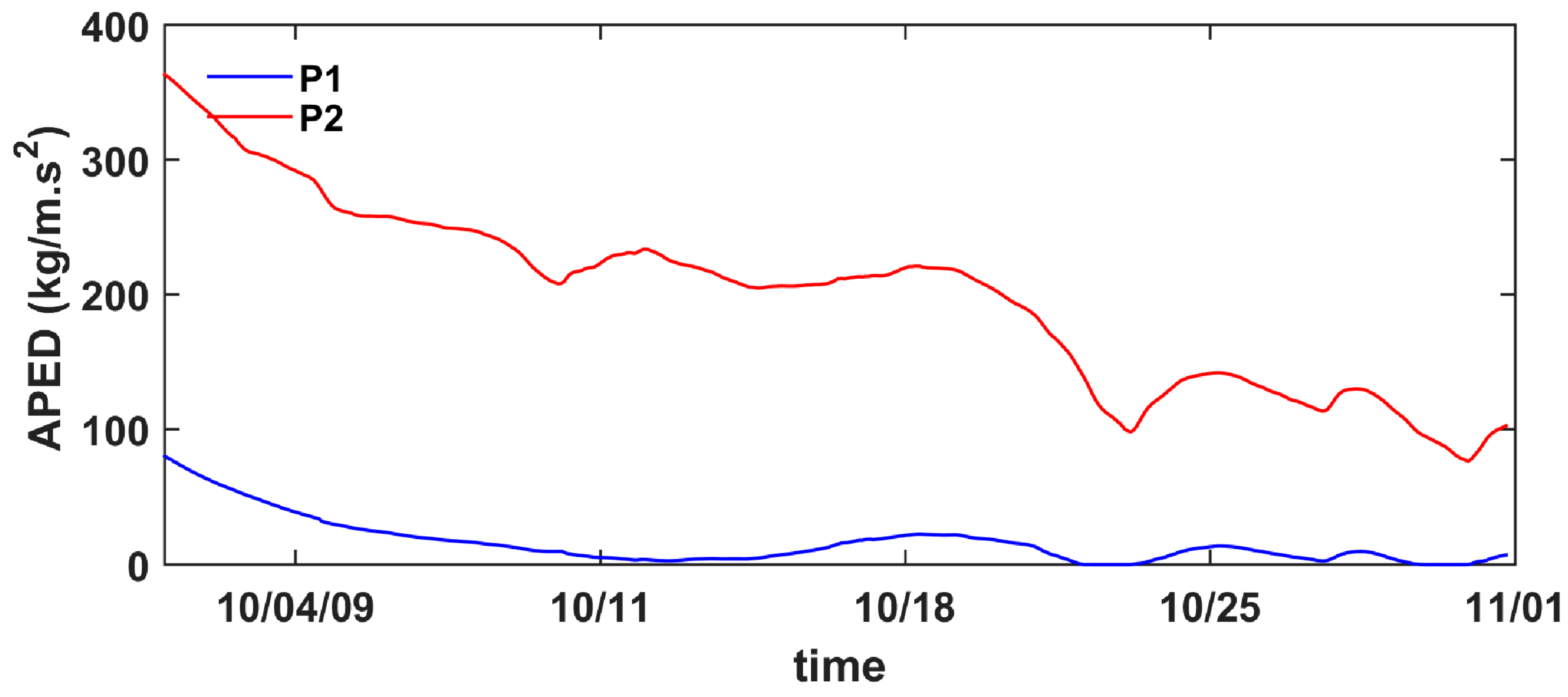
To further investigate the mixing and stratification state at P1 and P2, the average potential energy demand (APED) across the water column (the energy required per horizontal area for a complete vertical mixing) was calculated at each location [34,35] based on the simulated temperature and salinity across the water column:

$$\varphi =\frac{1}{h} \underset{-h}{\overset{\zeta }{\int }}(\overline{\rho }-\rho ) g z dz$$

(3)

In this equation, h is the total static water depth, $\zeta$ is water level above the static depth, $\overline{\rho }$ is the average water density across the water column, $\rho$is water density at each specific depth, g is gravitational acceleration (9.81 m²/s), and z is the vertical coordinate. The temporal variations of this parameter provide the information about the overall water column stratification through time [34,35]. Calculated time series of APED at stations P1 and P2 are compared in Figure 14. At both stations the time variation shows a decreasing trend demonstrating that, under the effect of several consecutive cold fronts, water columns at both stations are becoming more and more mixed, although, due to the smaller water depth and likely more active hydrodynamics, APED at P1 is much smaller and at times is close to zero, which demonstrates a fully mixed water column, as shown in Figure 12. At P1, APED at the beginning of simulation (1 October) was 80 Kg/m.s² and decreased to 5 kg/m.s² at the end of simulation (31 October), while at P2 the start and end values were 370 and 100, respectively, showing a more stable stratification across the water column at this station. The occasional increase in APED may have corresponded to the changes in wind direction and magnitude.

We did not analyze the direct effect of the cold front strength and/or duration of the previous cold front events on the duration of the mixing effect of the next cold front since this would require more numerical experiences and sensitivity analysis by changing the intensity of the cold fronts to different values and examining the results, which was not in the scope of this study. However, what can be implied from Figure 12 and Figure 13 is that the pre-storm state of shelf stratification can be crucial for the amount of mixing caused by the next events.

6. Conclusions

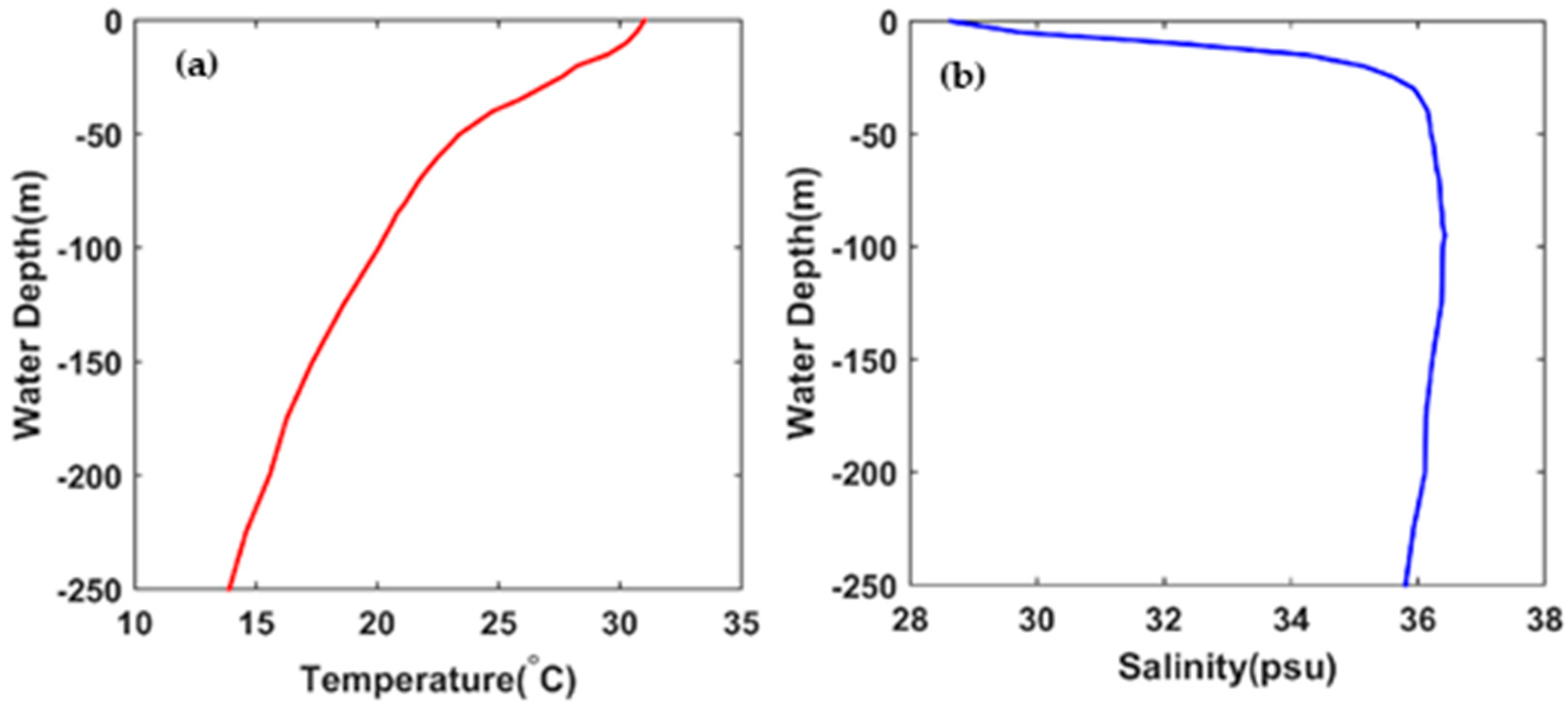
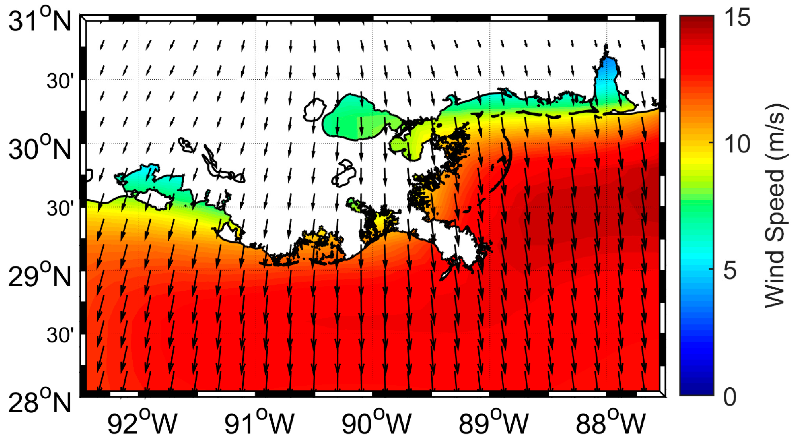
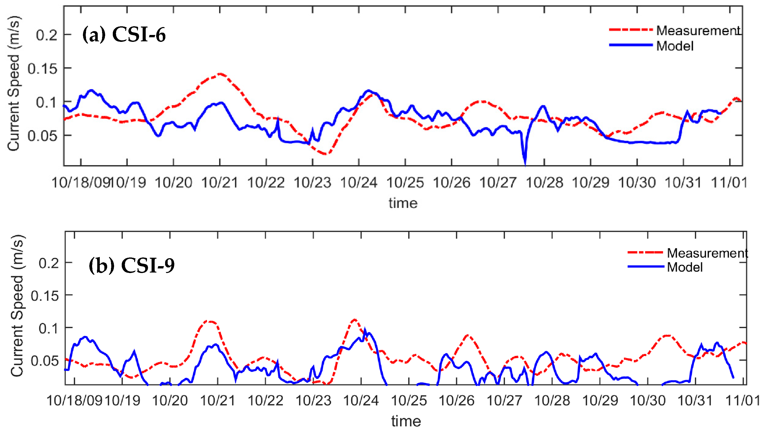
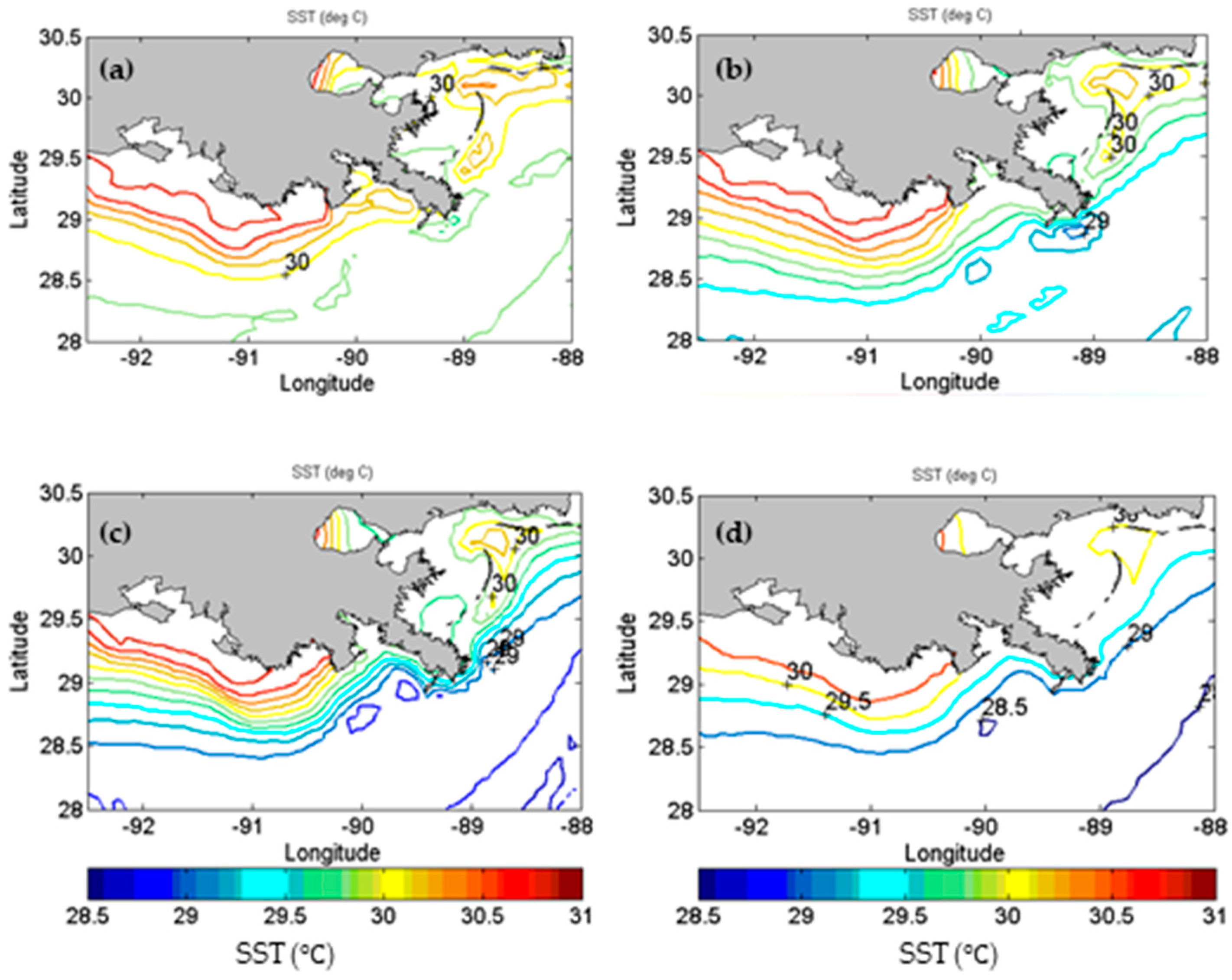
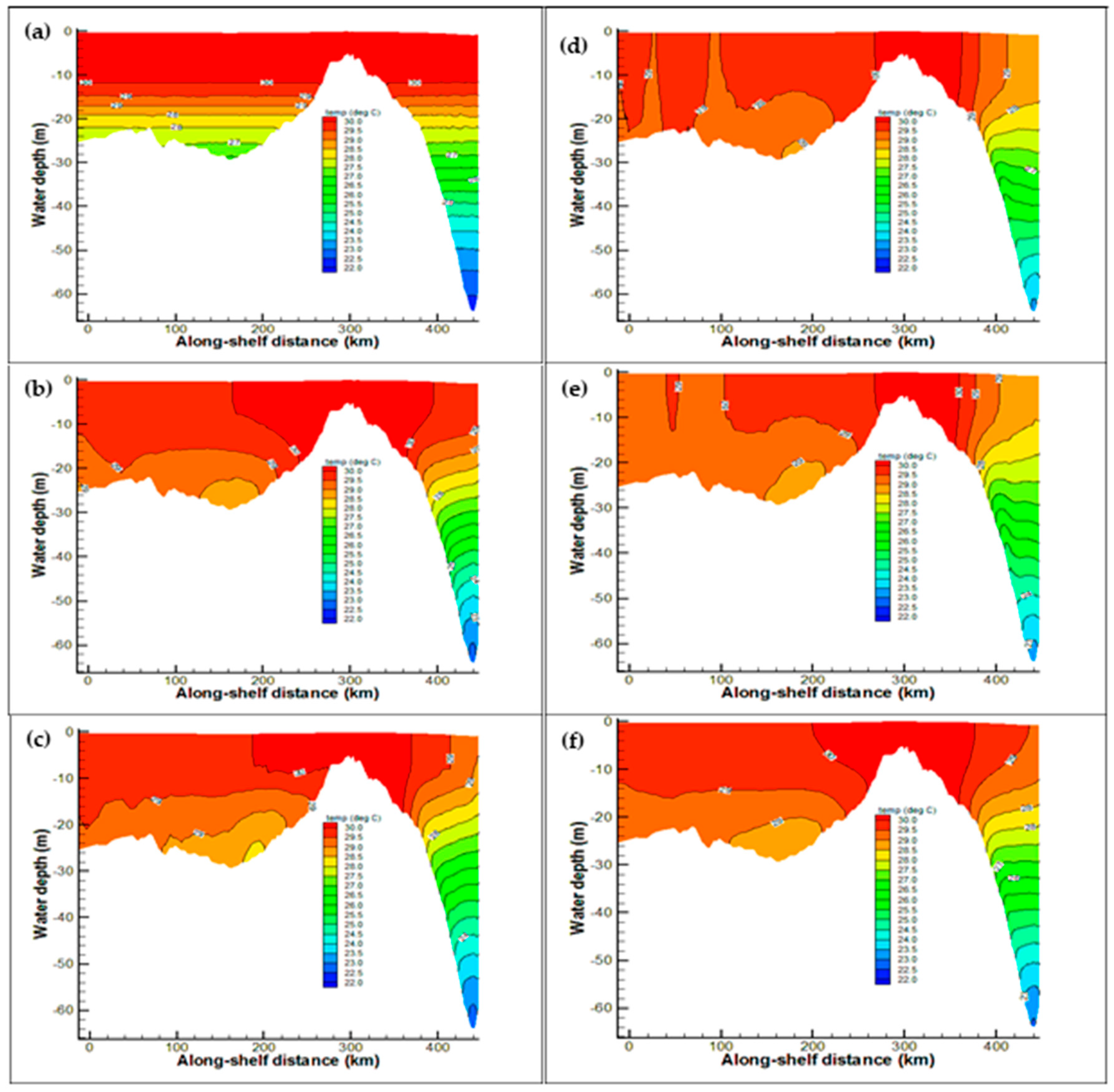
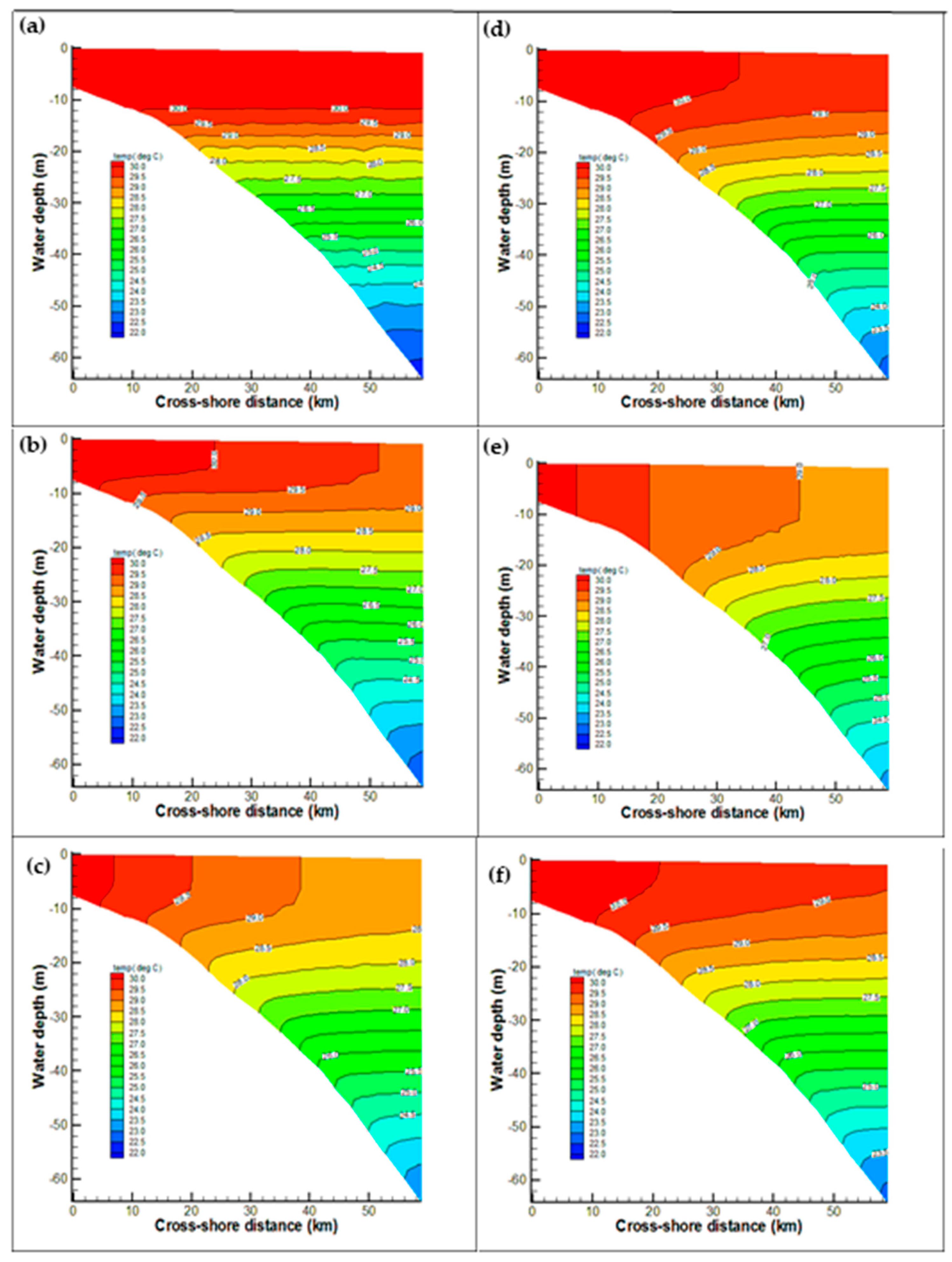
A numerical experiment was implemented to examine the mixing effect of a series of cold front events on water column stratification over the Louisiana continental shelf during October 2009. The experiment only included wind as the model forcing, and no solar radiation was used. The model hydrodynamics was verified using the measured de-tided currents at the WAVIS stations CSI-6 and CSI-9. Climatological profiles of temperature and salinity as the only available data were used to introduce the model’s initial stratification. This is reasonable because the main purpose was examining the stratification breakdown by the onset of strong cold fronts in the fall season. Model hydrodynamics showed relatively large surface currents (up to 0.3 m/s) after the passage of the cold fronts. The surface current followed the wind. The consecutive cold events caused a continuous decrease in SST, with the largest drop of SST over the Mississippi Bight and the deep shelf on the southwest of the Bird’s Foot Delta. Vertical profiles of temperature both along and across shelf cross-sections showed that, during and right after the cold front events, the water column started to mix, and the mixing depth over the shelf increased to 15–20 m depending on the location and the intensity of the storm. The mixing process significantly decreased before the next frontal passage. The stratification and mixing process were quantified at two locations over the shelf by calculating the mid-depth Richardson number and buoyancy frequency. The variation trends for both parameters at the two stations were decreasing, meaning the stratification was weakening, while their SST decreased between 1 °C and 1.5 °C during the simulation time due to the shelf mixing process. It was shown that the minimum values for both parameters occurred after the cold front event or before the next frontal passage. Two fully mixed water column events were observed for the station off Terrebonne/Timbalier Bay (water depth of 20 m), with the Richardson number being smaller than 0.25 and even close to zero. For the other station with a water depth of 30 located in the Mississippi Bight, the Richardson number was decreasing from the very stable stratification of 45 at the beginning of the simulation to less than 5 at the end of the one-month simulation. In addition to the Richardson number and buoyancy frequency, the average potential energy demand (APED) was calculated as a quantity across the water column at each station showing the amount of energy per unit area across the water column needed for a full water column mixing. This parameter also showed a trend of significant decreasing under the impact of repeated cold fronts. At P1 with a smaller water depth and more active hydrodynamics, the APED varied between 80 kg/m.s² at the start of simulation and 5 kg/m.s² at the end, respectively, with occasional zero values, while much larger energies were required to make a fully mixed water column at P2 (370 kg/m.s² at the start and 100 kg/m.s² at the end of simulation).

The results of this numerical experiment clearly showed the mixing effect of the winds associated with consecutive cold front events over the Louisiana shelf in destroying the strong stratification established in the summer over the Louisiana shelf. These winds, usually starting in mid-September, along with the decrease in solar radiation, can significantly mix the water column over the shelf and modulate the biogeochemical processes, including oxygen dynamics. It should be noted that cold fronts, as specified by their naming, are associated with cold air outbreak over the region and intense decrease in air temperature. This causes an increase in the heat loss at the water surface and decreases in the SST, which is a step toward a more mixed water column. Low heat loss at the surface can actually cause a strong stratification over the Louisiana shelf, as reported by Allahdadi and Li [36].

Although these northeasterly to northwesterly winds occur annually between September and May, the changes in their characteristics, including speed, direction, duration, and the occurrence interval imposed by different local and global atmospheric changes, can change the characteristics of mixing and the associated processes over the Louisiana shelf. Therefore, the effect of El Nino, La Nina, and climate change on these events and their implication for shelf mixing deserve to be investigated.

References

1. Wang, L.; Justić, D. A modeling study of the physical processes affecting the development of seasonal hypoxia over the inner Louisiana-Texas shelf: Circulation and stratification. Cont. Shelf Res. 2009, 29, 1464–1476. [Google Scholar] [CrossRef]
2. Allahdadi, M.N.; Jose, F.; Patin, C. Seasonal Hydrodynamics along the Louisiana Coast: Implications for Hypoxia Spreading. J. Coast. Res. 2013, 29, 1092–1100. [Google Scholar] [CrossRef]
3. Turner, R.E. Variability in the discharge of the Mississippi River and tributaries from 1817 to 2020. PLoS ONE 2022, 17, e0276513. [Google Scholar] [CrossRef] [PubMed]
4. Allison, M.A.; Kineke, G.C.; Gordon, E.S.; Goni, M.A. Development and reworking of a seasonal flood deposit on the inner continental shelf off the Atchafalaya River. Cont. Shelf Res. 2000, 20, 2267–2294. [Google Scholar] [CrossRef]
5. Sanial, V.; Shiller, A.M.; Joung, D.; Ho, P. Extent of Mississippi River water in the Mississippi Bight and Louisiana Shelf based on water isotopes. Estuarine. Coast. Shelf Sci. 2019, 226, 106196. [Google Scholar] [CrossRef]
6. Jansen, M.F. Glacial ocean circulation and stratification explained by reduced atmospheric temperature. Proc. Natl. Acad. Sci. USA 2017, 114, 45–50. [Google Scholar] [CrossRef] [Green Version]
7. Koohestani, K.; Allahdadi, M.N.; Chaichitehrani, N. Oceanic Response to Tropical Cyclone Gonu (2007) in the Gulf of Oman and the Northern Arabian Sea: Estimating Depth of the Mixed Layer Using Satellite SST and Climatological Data. J. Mar. Sci. Eng. 2021, 9, 1244. [Google Scholar] [CrossRef]
8. McGee, L.; He, R. Mesoscale and submesoscale mechanisms behind asymmetric cooling and phytoplankton blooms induced by hurricanes: A comparison between an open ocean case and a continental shelf sea case. Ocean. Dyn. 2018, 68, 1443–1456. [Google Scholar] [CrossRef] [Green Version]
9. Zhang, J.L.; Steele, M. Effect of vertical mixing on the Atlantic water layer circulation in the Arctic Ocean. J. Geophys. Res. Ocean. 2007, 112, 1.e9. [Google Scholar] [CrossRef]
10. Keen, T.R.; Glenn, S.M. Factors influencing model skill for hindcasting shallow water currents during Hurricane Andrew. J. Atmos. Ocean. Technol. 1998, 15, 221.e236. [Google Scholar] [CrossRef]
11. Matli, V.R.R.; Fang, S.; Guinness, J.; Rabalais, N.N.; Craig, J.K.; Obenour, D.R. Space-Time Geostatistical Assessment of Hypoxia in the Northern Gulf of Mexico. Environ. Sci. Technol. 2018, 52, 12484–12493. [Google Scholar] [CrossRef]
12. Scavia, D.; Bertani, I.; Obenour, D.R.; Turner, R.E.; Forrest, D.R.; Katin, A. Ensemble modeling informs hypoxia management in the northern Gulf of Mexico. Proc. Natl. Acad. Sci. USA 2017, 114, 8823–8828. [Google Scholar] [CrossRef] [Green Version]
13. Rabalais, N.N.; Baustian, M.M. Historical Shifts in Benthic Infaunal Diversity in the Northern Gulf of Mexico since the Appearance of Seasonally Severe Hypoxia. Diversity 2020, 12, 49. [Google Scholar] [CrossRef] [Green Version]
14. Rabalais, N.N.; Turner, R.E. Gulf of Mexico Hypoxia: Past, Present, and Future. Limnol. Oceanogr. Bull. 2019, 28, 117–124. [Google Scholar] [CrossRef] [Green Version]
15. Scavia, D.; Justić, D.; Obenour, D.R.; Craig, J.K.; Wang, L. Hypoxic volume is more responsive than hypoxic area to nutrient load reductions in the northern Gulf of Mexico—And it matters to fish and fisheries. Environ. Res. Lett. 2019, 14, 024012. [Google Scholar] [CrossRef]
16. Allahdadi, M.N.; Li, C.; Chaichitehrani, N. Numerical Experiments of Temperature Mixing and Post-Storm Re-Stratification over the Louisiana Shelf during Hurricane Katrina (2005). J. Mar. Sci. Eng. 2022, 10, 1082. [Google Scholar] [CrossRef]
17. Chaichitehrani, N.; Allahdadi, M.N. Overview of Wind Climatology for the Gulf of Oman and the Northern Arabian Sea. Am. J. Fluid Dyn. 2018, 8, 1–9. [Google Scholar]
18. Romero-Arteaga, A.; Ruiz de Alegría-Arzaburu, A.; Rivas, D.; Juarez, B. Nearshore current variations during the passage of cold fronts in NW Gulf of Mexico. Cont. Shelf Res. 2022, 238, 104697. [Google Scholar] [CrossRef]
19. Romero-Arteaga, A.; Ruiz de Alegría-Arzaburu, A. Spatial variability of currents associated with different cold fronts along the southern Texas coast. Ocean. Dyn. 2022, 72, 279–294. [Google Scholar] [CrossRef]
20. Li, C.; Weeks, E.; Huang, W.; Milan, B.; Wu, R. Weather-induced transport through a tidal channel calibrated by an unmanned boat. J. Atmos. Ocean. Technol. 2017, 35, 261–279. [Google Scholar] [CrossRef]
21. Lin, J.; Li, C.; Boswell, K.M.; Kimball, M.; Rozas, L. Examination of winter circulation in a northern Gulf of Mexico estuary. Estuar. Coasts 2016, 39, 879–899. [Google Scholar] [CrossRef]
22. Li, C.; Chen, C. Shelf circulation prior to and post a cold front event measured from vessel-based acoustic Doppler current profiler. J. Mar. Syst. 2014, 139, 38–50. [Google Scholar] [CrossRef]
23. Feng, Z.; Li, C. Cold-front-induced flushing of the Louisiana Bays. J. Mar. Syst. 2010, 82, 252–264. [Google Scholar] [CrossRef]
24. Allahdadi, M.N.; Jose, F.; D’Sa, E.J.; Ko, D.S. Effect of wind, river discharge, and outer-shelf phenomena on circulation dynamics of the Atchafalaya Bay and shelf. Ocean. Eng. 2017, 129, 567–580. [Google Scholar] [CrossRef]
25. Chen, C.S.; Beardsley, R.C.; Cowles, G. An Unstructured Grid, Finite-Volume Coastal Ocean Model, FVCOM User Manual; University of Massachusetts, Dartmouth: New Bedford, MA, USA, 2006. [Google Scholar]
26. Pan, J.; Sun, Y. Estimate of Ocean Mixed Layer Deepening after a Typhoon Passage over the South China Sea by Using Satellite Data. J. Phys. Oceanogr. 2012, 43, 498–506. [Google Scholar] [CrossRef]
27. Chaichitehrani, N.; Allahdadi, M.N.; Li, C. Simulation of Low Energy Waves during Fair-Weather Summer Conditions in the Northern Gulf of Mexico: Effect of Whitecapping Dissipation and the Forcing Accuracy. Atmosphere 2022, 13, 2047. [Google Scholar] [CrossRef]
28. Zhang, Z.; Hetland, R.; Zhang, X. Wind-modulated buoyancy circulation over the Texas-Louisiana shelf. J. Geophys. Res. Ocean. 2014, 119, 5705–5723. [Google Scholar] [CrossRef]
29. Allahdadi, M.N.; Li, C. Numerical Simulation of Louisiana Shelf Circulation under Hurricane Katrina. J. Coast. Res. 2018, 34, 67–80. [Google Scholar] [CrossRef]
30. Lyons, R.; Panofsky, H.A.; Wollaston, S. The critical Richardson number and its implication for forecast problems. J. Appl. Meteorol. 1964, 3, 136–142. [Google Scholar] [CrossRef]
31. Turner, J.S. Buoyancy Effects in Fluids; Cambridge University Press: Cambridge, UK, 1973; p. 367. [Google Scholar]
32. Galperin, B.; Sukoriansky, S.; Anderson, P.S. On the critical Richardson number in stably stratified turbulence. Atmos. Sci. Lett. 2007, 8, 65–69. [Google Scholar] [CrossRef]
33. Huguenard, K.D.; Bogucki, D.J.; Ortiz-Suslow, D.G.; MacMahan, J.H. Nearshore response to cold air outbreaks in the Gulf of Mexico. Estuarine. Coast. Shelf Sci. 2020, 235, 106604. [Google Scholar] [CrossRef]
34. Li, C.; Swenson, E.; Weeks, E.; White, J.R. Asymmetric tidal straining across an inlet: Lateral inversion and variability over a tidal cycle. Estuar. Coast. Shelf Sci. 2009, 85, 651–660. [Google Scholar] [CrossRef]
35. Simpson, J.H.; Brown, J.; Matthews, J.; Allen, G. Tidal straining, density currents, and stirring in the control of estuarine stratification. Estuaries 1990, 13, 125–132. [Google Scholar] [CrossRef]
36. Allahdadi, M.N.; Li, C. Numerical experiment of stratification induced by diurnal solar heating over the Louisiana shelf. In Modeling Coastal Hypoxia: Numerical Simulations of Patterns, Controls and Effects of Dissolved Oxygen Dynamics, 1st ed.; Justic, D., Rose., K., Hetland, R., Fennel, K., Eds.; Springer: Berlin/Heidelberg, Germany, 2017; Chap 1. [Google Scholar]
Figure 1. (a) Location of the Louisiana shelf (the black box) in the northern Gulf of Mexico, (b) A close view of the Louisiana shelf geographical extent. The horizontal black line (LS 1) is the along-shelf section later used to examine the simulated temperatures across the water column. The red north–south line is the cross-section A used to represent temperature results across the water column. The location of station CSI-6 used for evaluation of the hydrodynamics model is shown by a star. AB: Atchafalaya Bay, TB: Terrebonne/Timbalier Bay, and BB: Barataria Bay.
Jmse 11 00673 g001
Figure 2. (a) Modeling area and bathymetry, (b) computational mesh. MB in panel (a) stands for Mississippi Bight.
Jmse 11 00673 g002
Figure 3. Temperature (a) and salinity (b) profiles from the WOA database for September at a location on the Louisiana shelf off Terrebonne Bay.
Jmse 11 00673 g003
Figure 4. A sample of CFSR wind filed during the peak of cold front no.2 over the Louisiana shelf.
Jmse 11 00673 g004
Figure 5. Time series of wind vectors measured at CSI-6 during October 2009, (a) wind speed, (b) wind direction, and (c) wind vectors. The numbered arrows in panel (c) show the approximate time corresponding to each of the five cold front events in October 2009.
Jmse 11 00673 g005
Figure 6. Comparison of simulated current speed and measured de-tided current speed at (a) CSI-6 and, (b) CSI-9.
Jmse 11 00673 g006
Figure 7. Simulated wind-induced surface currents over the Louisiana shelf during and after different cold front events, (a) 10 October 12:00 a.m., (b) 17 October 12:00 a.m., (c) 22 October 12:00 a.m., (d) 27 October 12:00 a.m.
Jmse 11 00673 g007
Figure 8. Simulated SST over the Louisiana shelf after different cold front events, (a) 10 October 12:00 a.m., (b) 17 October 12:00 a.m., (c) 22 October 12:00 a.m., (d) 27 October 12:00 a.m.
Jmse 11 00673 g008
Figure 9. Satellite OI SST maps over the Louisiana shelf at times corresponding to the different cold front events in October 2009.
Jmse 11 00673 g009
Figure 10. Distribution of simulated temperature across section AS 1 (see Figure 1 for location) on (a) 1 October, (b) 10 October, (c) 17 October, (d) 22 October, (e) 27 October, (f) 1-month average. All snapshots from a) to (e) were taken at 12:00 a.m.
Jmse 11 00673 g010
Figure 11. Distribution of simulated temperature across transect A (Figure 1 for location) (a) 1 October, (b) 10 October, (c) 17 October, (d) 22 October, (e) 27 October, (f) 1-month average.
Jmse 11 00673 g011
Figure 12. Variations of SST and water temperature across the water column during one-month simulation in October 2009 for: (left panels) station P1 and (right panel) station P2. Location of stations is based on Figure 1.
Jmse 11 00673 g012
Figure 13. Variations of buoyancy frequency and the Richardson number across the water column during one-month simulation during October 2009 for: (left panels) station P1 and (right panel) station P2. The red dash line shows the trend of the Richardson number variations during the simulation.
Jmse 11 00673 g013
Figure 14. Time variations of calculated APED at locations P1 and P2.
Jmse 11 00673 g014
Disclaimer/Publisher’s Note: The statements, opinions and data contained in all publications are solely those of the individual author(s) and contributor(s) and not of MDPI and/or the editor(s). MDPI and/or the editor(s) disclaim responsibility for any injury to people or property resulting from any ideas, methods, instructions or products referred to in the content.