Automated Atmospheric Correction of Nanosatellites Using Coincident Ocean Color Radiometer Data

Abstract

Here we present a machine-learning-based method for utilizing traditional ocean-viewing satellites to perform automated atmospheric correction of nanosatellite data. These sensor convolution techniques are required because nanosatellites do not usually possess the wavelength combinations required to atmospherically correct upwelling radiance data for oceanographic applications; however, nanosatellites do provide superior ground-viewing spatial resolution (~3 m). Coincident multispectral data from the Suomi National Polar-Orbiting Partnership Visible Infrared Imaging Radiometer Suite (Suomi NPP VIIRS; referred to herein as “VIIRS”) were used to remove atmospheric contamination at each of the nanosatellite’s visible wavelengths to yield an estimate of spectral water-leaving radiance [L_w(l)], which is the basis for surface ocean optical products. Machine learning (ML) algorithms (KNN, decision tree regressors) were applied to determine relationships between L_w and top-of-atmosphere (L_t)/Rayleigh (L_r) radiances within VIIRS training data, and then applied to test cases for (1) the Marine Optical Buoy (MOBY) in Hawaii and (2) the AErosol RObotic Network Ocean Color (AERONET-OC), Venice, Italy. For the test cases examined, ML-based methods appeared to improve statistical results when compared to alternative dark spectrum fitting (DSF) methods. The results suggest that ML-based sensor convolution techniques offer a viable path forward for the oceanographic application of nanosatellite data streams.

1. Introduction

The prevailing mission-based paradigm for ocean color remote sensing typically involves high-cost satellite platforms launched and operated by government agencies such as NASA, NOAA, ESA, and JAXA. These platforms host state-of-the-art ocean-viewing radiometers with design and sensitivity specifications appropriate for delineating a comparatively weak water-leaving radiance from the total radiant signal detected at the top of the atmosphere. The current suite of such operational ocean color sensors includes NASA’s Moderate Resolution Imaging Spectroradiometer (MODIS; Aqua satellite), NOAA’s VIIRS (SNPP and NOAA-20 satellites), the Ocean and Land Colour Instrument (OLCI; Sentinel-3 A/B satellites), and the Second-Generation Global Imager (SGLI) onboard the GCOM-C satellite. All of these sensors provide multi-spectral band sets (visible, near-infrared (NIR), and shortwave infrared (SWIR)) with daily coverage at approximately kilometer-scale spatial resolution. However, even kilometer-scale spatial resolution may be unable to resolve finer-scale features near rivers and estuaries that are critical for scientific and environmental resource management applications.

In contrast to government-sponsored, large satellite missions, commercial entities are now deploying low-cost cubesats with much higher spatial resolution imaging capability. Planet Labs currently has ~200 (as of November 2022) orbiting nanosatellites that provide high-temporal-resolution monitoring of the Earth’s surface at a spatial resolution previously available only by the high-cost tasking of a few specialized satellites such as WorldView 3/4 [1]. The majority of these nanosatellites (known collectively as PlanetScope (PS)) host a multispectral digital camera with blue, green, red, and NIR bands, which image the earth at very high spatial resolution (3.125 m ground resolution at nadir). PS data have been used to monitor volcano activity [2], assess vegetative index [3,4], aid agriculture studies [5,6], study lake dynamics [7], determine high-resolution topography [8], detect oil spills [9], monitor rangeland [10], and monitor disasters [11]. PS applications for aquatic environments include monitoring coral reefs [12] and water quality [13,14], Sargassum detection [15], detection of river ice and water velocities [16], high-resolution bathymetry [17], and monitoring seagrass beds [18].

Other commercial groups are also exploiting nanosatellite technology for a wide variety of remote sensing applications [19,20,21,22,23]. However, there have been only a small number of studies to assess these commercial nanosatellite data sources as a viable solution for ocean color remote sensing, i.e., detection of the water-leaving radiant signal in the visible bands after removal of the intervening atmospheric contamination [24]. Maciel et al. studied the potential for cubesats to provide remote sensing reflectance over very turbid inland lakes [25]. Vanhellemont applied the dark spectrum fitting (DSF) aerosol correction method [26,27] to PS data [14] and also found success in the PS red bands over very turbid waters.

More generalized ocean color applications of PS data will require removal of the atmospheric portion of the total sensor signal at the top of the atmosphere. Nearly 30 years ago, Gordon and Wang set the standard for atmospheric correction by using a relationship between two relatively narrow NIR or SWIR bands to estimate the aerosol radiance contribution in a satellite’s total path radiance, Lt [28,29]. The use of two NIR bands is still one of the primary methods used today for characterizing and removing the aerosol radiance during atmospheric correction. However, the design of many small satellites is focused on terrestrial observation, and these sensors do not have the NIR/SWIR wavelengths needed for the standard method of atmospheric correction for ocean color. This inadequacy suggests that alternative methods should be explored for atmospheric correction [30,31]. In this paper, we present an alternative atmospheric correction method in order to exploit PS data for ocean color applications. We selected machine learning (ML)-based techniques as a means to convolve data from traditional ocean color sensors, which permit a complete atmospheric correction, with PS data that are otherwise inadequate for this purpose.

2. Materials and Methods

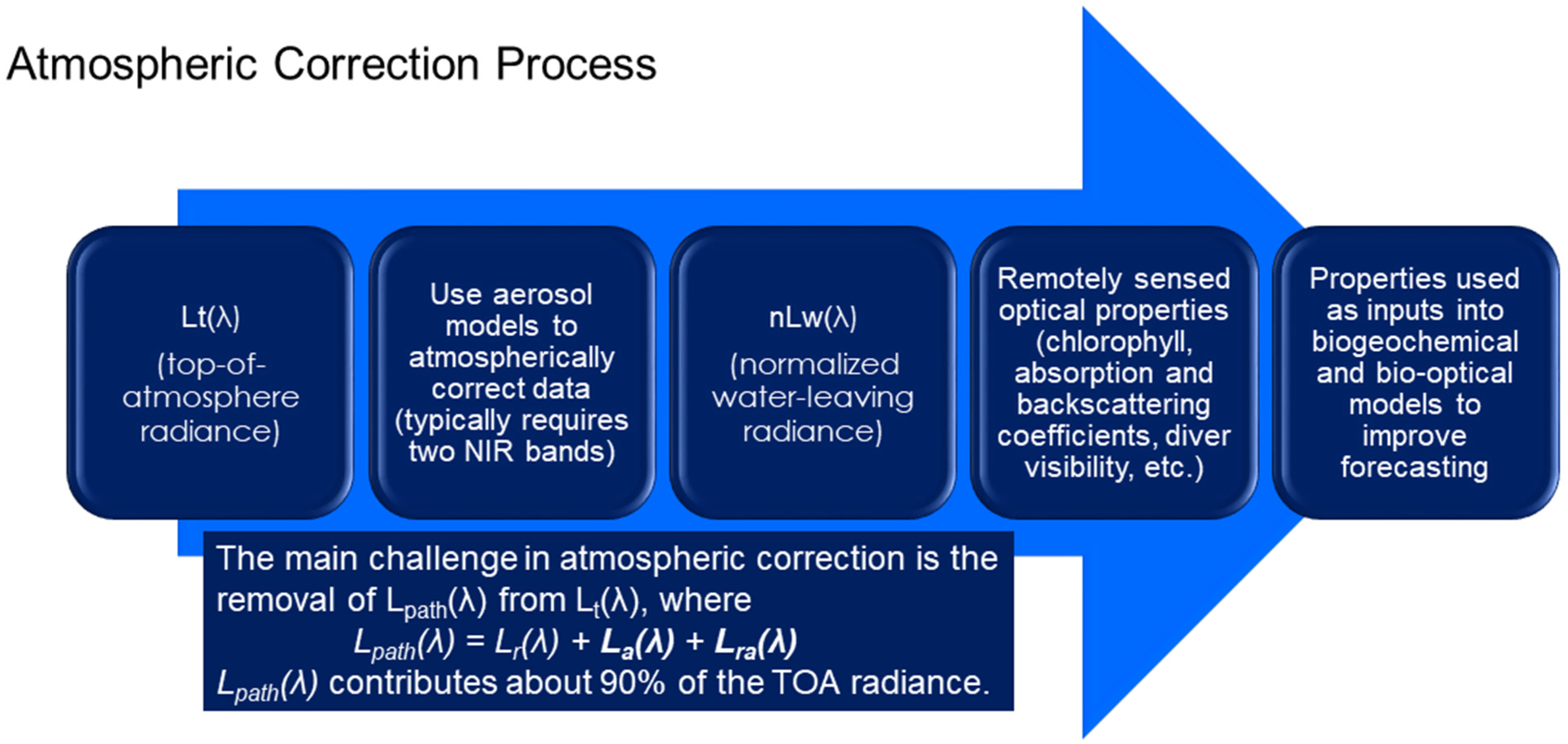
The lack of NIR/SWIR bands in PS data, as well as most other small satellites launched primarily to monitor land, represents a challenge in performing atmospheric correction. Roughly 90% of the total Lt recorded by the satellite represents atmospheric radiance and must be removed prior to calculating Lw, and ultimately the follow-on products, whichinclude bio-optical water properties. The atmospheric signal consists of Rayleigh scattering (Lr, scattering by molecules, calculated from sensor viewing geometry) and aerosol scattering (La, modeled from radiances in two NIR/SWIR bands). Typical coarse-resolution ocean color sensors such as MODIS, VIIRS, SGLI, and Sentinel-3 OLCI have 9, 11, and 21 bands, respectively, two or more of which are at NIR or SWIR wavelengths needed to atmospherically correct the visible bands. These types of sensors are equipped with bands that are fairly narrow, roughly 15–20 nm in bandwidth. For the PS nanosatellites, however, there are typically only 4–5 bands available, with broader bandwidths (60–90 nm) and only one NIR band. Planet has started to launch flocks of “Super Dove” nanosatellites equipped with an additional red-edge band (705 nm) that could potentially aid in improved atmospheric correction, at least in open ocean areas where the signal is dominated by water. Thus, while it is promising that PlanetScope nanosatellites and other small satellites typically have 1 NIR band and current and future “Super Dove” nanosatellites possess a red-edge band, scientific challenges exist due to the lack of additional bands required for correction routines.

The Hyperspectral Imager for the Coastal Ocean (HICO) was a sensor developed by the Naval Research Laboratory (NRL) and housed on the International Space Station from late 2009 to 2014 [32]. It measured Lt from 352 to 1079 nm at a bandwidth of about 5 nm. In order to atmospherically correct HICO using the standard Gordon and Wang atmospheric correction, Rayleigh coefficient and aerosol model coefficient look up tables (LUTs) were developed for HICO by NASA’s Ocean Biology Processing Group (OBPG). In addition, values for other required parameters for processing Planet nanosatellite data, such as solar irradiance, Rayleigh optical depth, and the absorption and backscatter of pure water, were available at 1 nm intervals. These LUT coefficients and values were convolved against the Planet Relative Spectral Response (RSR) functions to generate the Rayleigh and aerosol model tables and other coefficients representative of the Planet bands’ wavelength characteristics. Additionally, not every Planet nanosatellite has the same RSR. The RSR varies depending on the flock (group of nanosatellites that are built and launched together), which can lead to different center wavelengths during the convolving process (e.g., red wavelength centered at 635 nm for the PlanetScope “0F” Series and 644 nm for the PlanetScope “E” Series).

There is a difference between the wavelength centers of the closest Planet and VIIRS bands.

Table 1. Blue, green, and red Center Wavelengths for VIIRS and Planet’s PlanetScope Nanosatellites.

Color	VIIRS Center Wavelength	Nanosatellite Center Wavelength
Blue	486 nm	“0C” and “0D” series: 490 nm (not in this study) “10”, “0E”, and “0F” series: 494 nm
Green	551 nm	All series: 545 nm
Red	671 nm	“10” and “0F” series: 635 nm “0E” series: 644 nm “0C and “0D” series: 649 nm (not in this study)

shows that the Planet nanosatellite center wavelengths are within 4–8 nm (when compared to VIIRS) for the blue band, 6 nm for the green band, and 27–36 nm for the red band. The variation in the blue and red bands represents the range of wavelengths in the 4 different series of the initial Planet sensors. The blue and green bands are close enough to the VIIRS center wavelengths to use coincident VIIRS imagery in building a model to atmospherically correct the nanosatellites, but the red band is likely too distant to be reliably used for this approach. All of the imagery from the nanosatellites used in this study were from the PlanetScope “10”, “0E”, and “0F” series. All three of these series have the blue band centered at 494 nm, but the “10” and “0F” series have the red band centered at 635 nm while the “0E” series is centered at 644 nm.

During this study, we demonstrate how we can atmospherically correct satellite sources, such as Planet nanosatellites, that are not primarily designed for ocean color remote sensing. We use two different methods and assess the result of each method. The first method uses the nanosatellites’ red and NIR bands to automatically select a pair of bounding aerosol models to remove the aerosol contribution from Lt within the visible bands. This method uses the traditional Gordon–Wang approach for aerosol model selection and the convoluted LUTs and parameters mentioned prior. The impact of using a red band as the first NIR band in data processing is that the signal in the red band is interpreted as aerosol radiance. As a result, if there is valid non-aerosol water leaving radiance such as in sediment-laden waters, the estimation of the aerosol component can be artificially high and the Lw estimates in the visible bands will be negatively impacted. This is more evident in the locations where the red band has higher signal, for example in turbid coastal waters. However, there is another artifact of this approach. During the Gordon–Wang atmospheric correction process, the signal in the second NIR band identified as “aer_wave_long” within the atmospheric correction module and red band in the cast of Planet data is iteratively reduced towards 0 during the execution of the algorithm. When using two true NIR bands, after atmospheric correction, the values in the two NIR bands will already be close to 0 even in turbid waters. This is irrelevant in further processing since those NIR bands are not used in ocean color bio-optical algorithms. However, in the case of the Planet datasets, this is a significant drawback since the red band, used as the “aer_wave_short” band, is needed for bio-optical algorithms. Therefore, this other artifact of using a red band as the “aer_wave_short” band in processing is that after processing there is almost no signal remaining in the red band to use in bio-optical ocean color algorithms.

In order to address the negative impact on the red band’s nLw value caused by using the red band as “aer_wave_short” in the atmospheric correction process, the red band in the Planet L1B file was duplicated, allowing one of the duplicated bands to participate as the “aer_wave_short” band and the other to participate as the visible red band to be used in ocean color bio-optical algorithms. The creation of the Planet standard L1B data files was adjusted to duplicate the red band. This resulted in a 5-band Planet L1B file with the 4th band being a duplication of the 3rd band. All supporting sensor data files were adjusted to accommodate for this duplication. The computation in processing then used the 4th and 5th bands as the “aer_wave_short” and “aer_wave_long” bands, leaving the 3rd band as a visible red band. The atmospheric correction process reduced the nLw values in the 4th and 5th bands towards 0 as it selected an aerosol model used to compute the aerosol radiance (La) estimate. Then, the La and Lr estimates were subtracted from the visible bands’ Lt measurements to compute their Lw and ultimately their nLw values. The 3rd band was treated as the visible red band in this process and its nLw values were computed along with the nLw estimates for the other two visible bands.

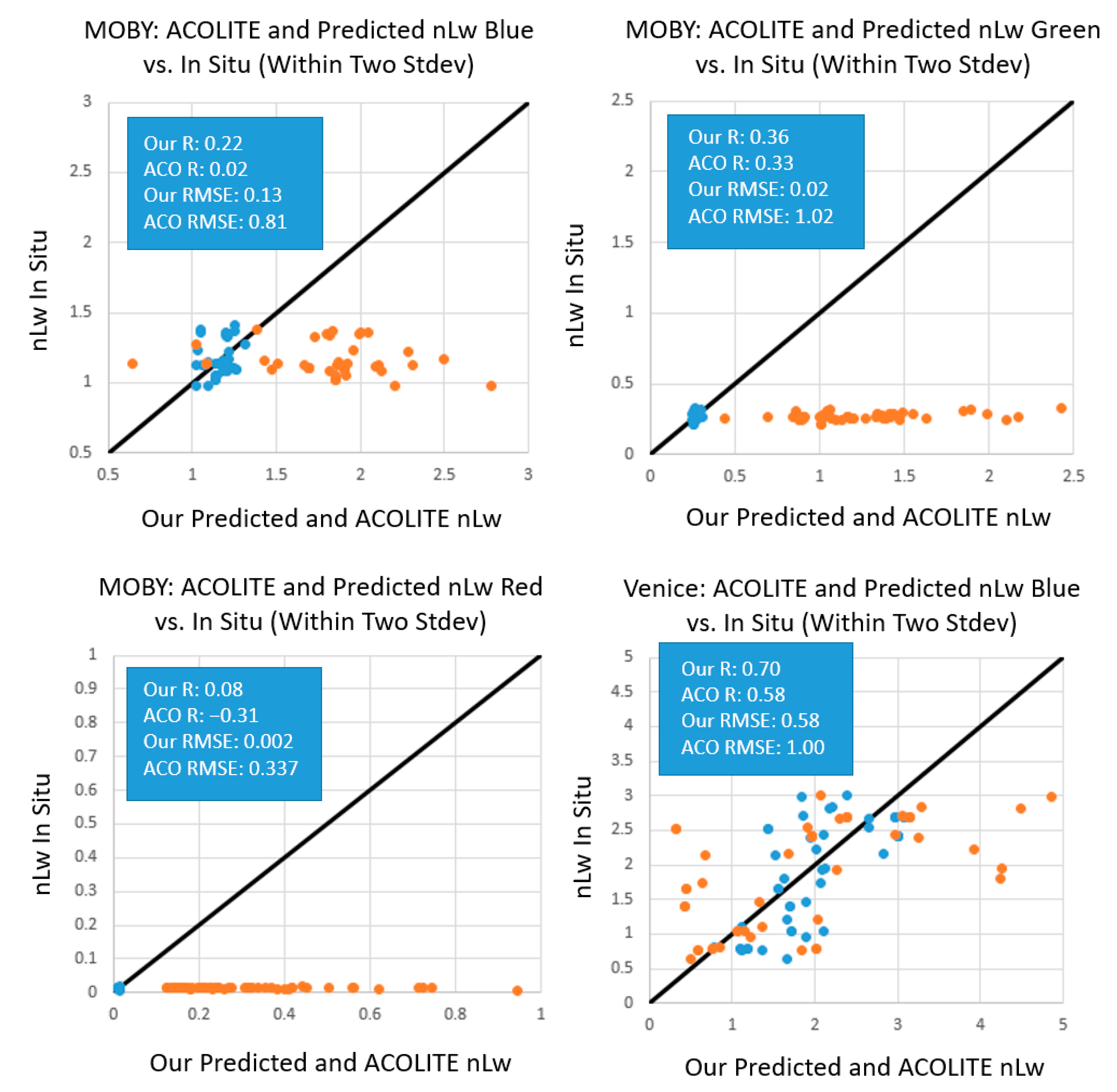
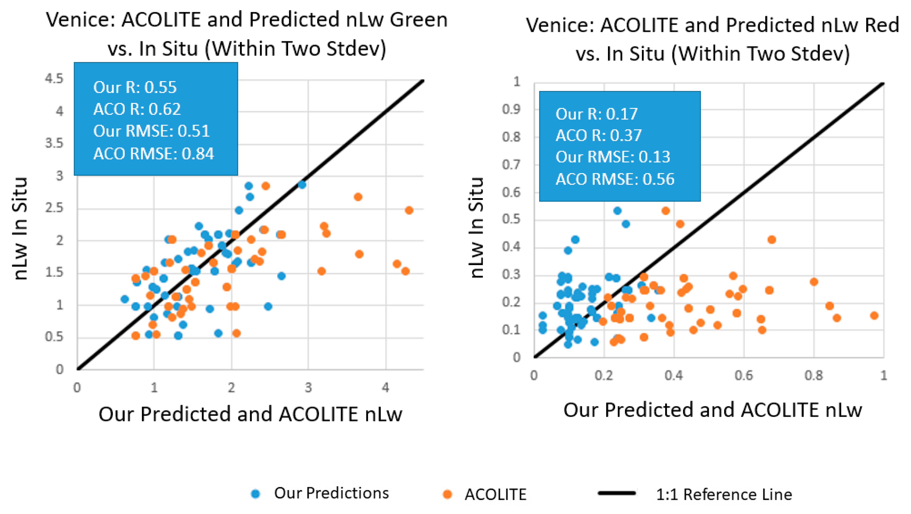
This solution yields a “baseline” for an automated solution to atmospherically correct imagery from satellites that do not have the required bands needed for atmospheric correction. The Gordon–Wang aerosol model selection process using two bands in the NIR/SWIR is very sensitive, so using the red band where the water-leaving radiance is greater than 0 leads to higher uncertainties in the derived water-leaving radiances. The second method for atmospherically correcting these datasets is to develop models that determine relationships between Lt, Lr, and nLw for each of the VIIRS’ visible bands that closely coincide with those from Planet’s nanosatellites. Once an atmospheric correction model was developed from VIIRS training values and evaluated against VIIRS values not within the training set, it was applied to the nanosatellite Lt and Lr values to predict nLw at any given pixel location within the scene that was geographically coincident to the training locations (MOBY and AERONET-OC Venice in situ locations). Finally, we compared our results to those produced from ACOLITE, which uses the dark spectrum fitting (DSF) atmospheric correction approach.

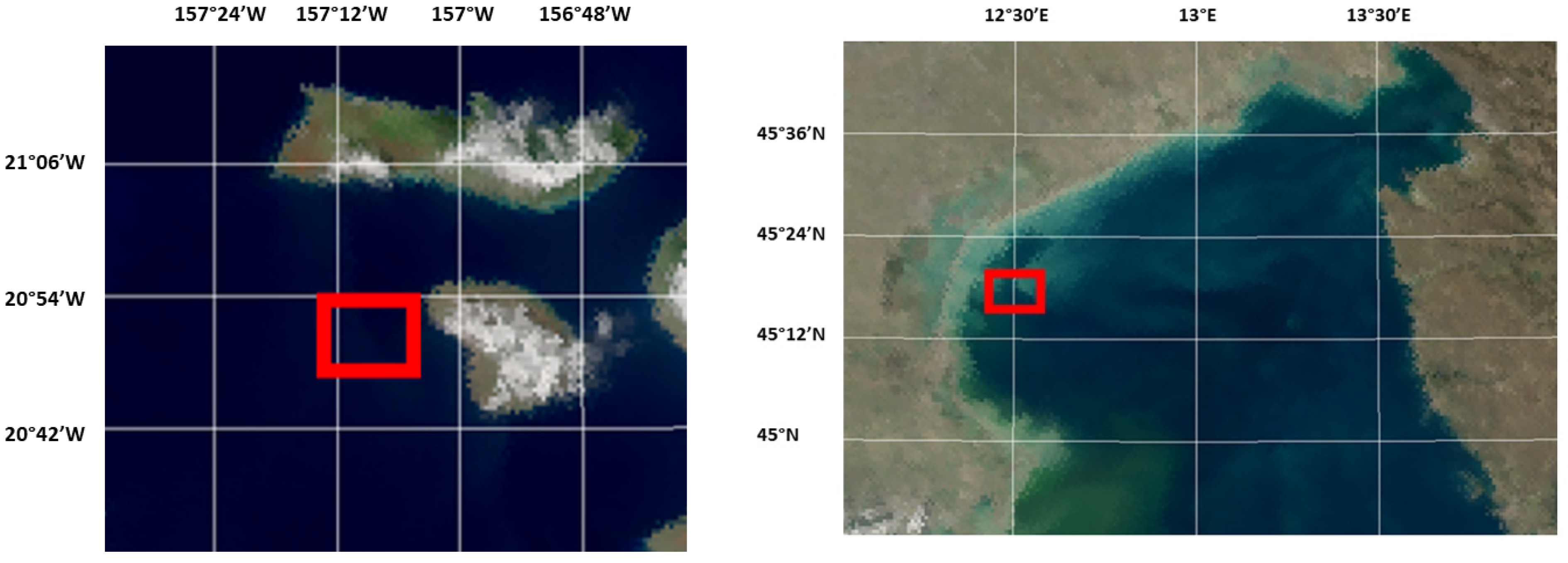
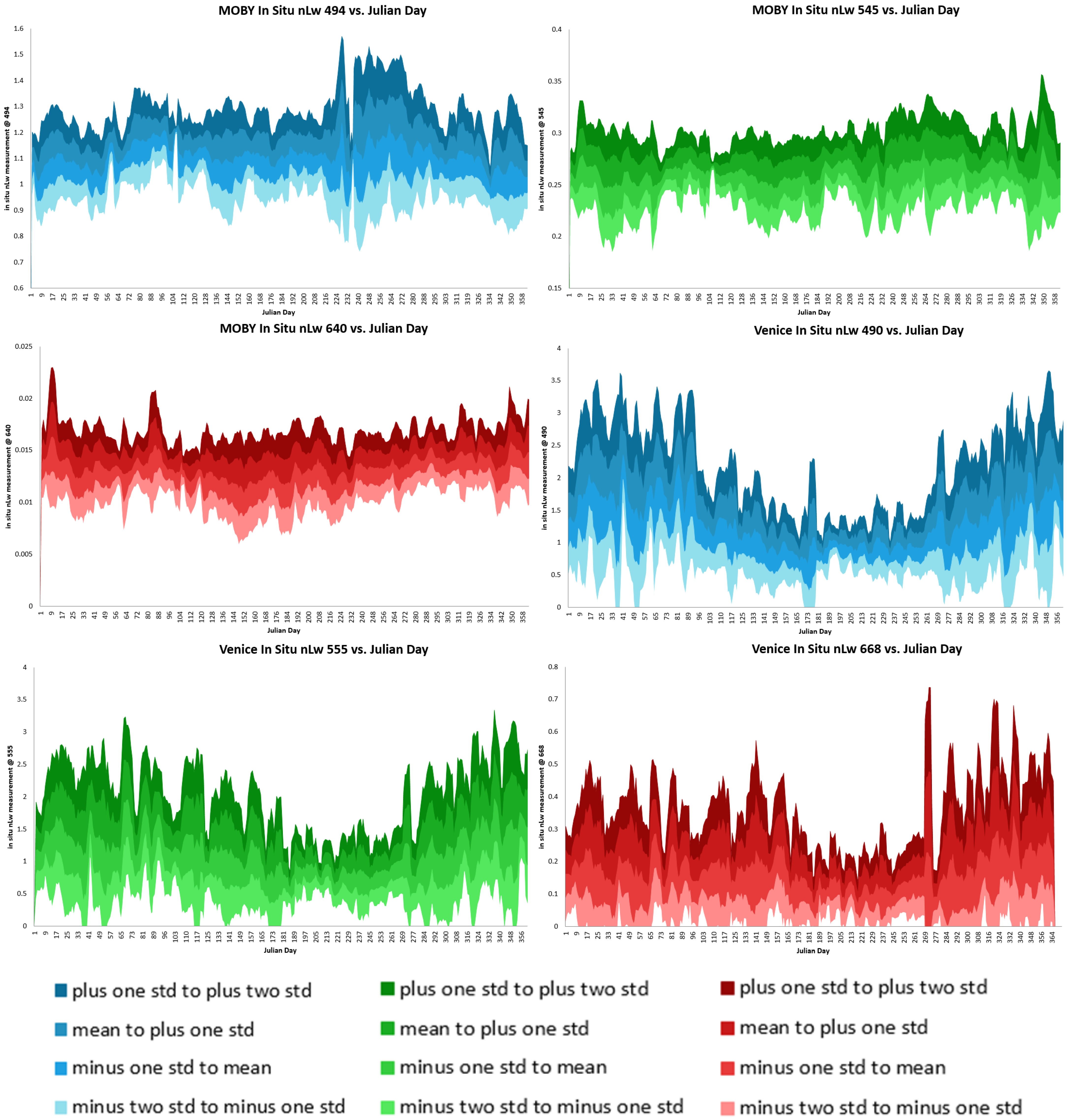
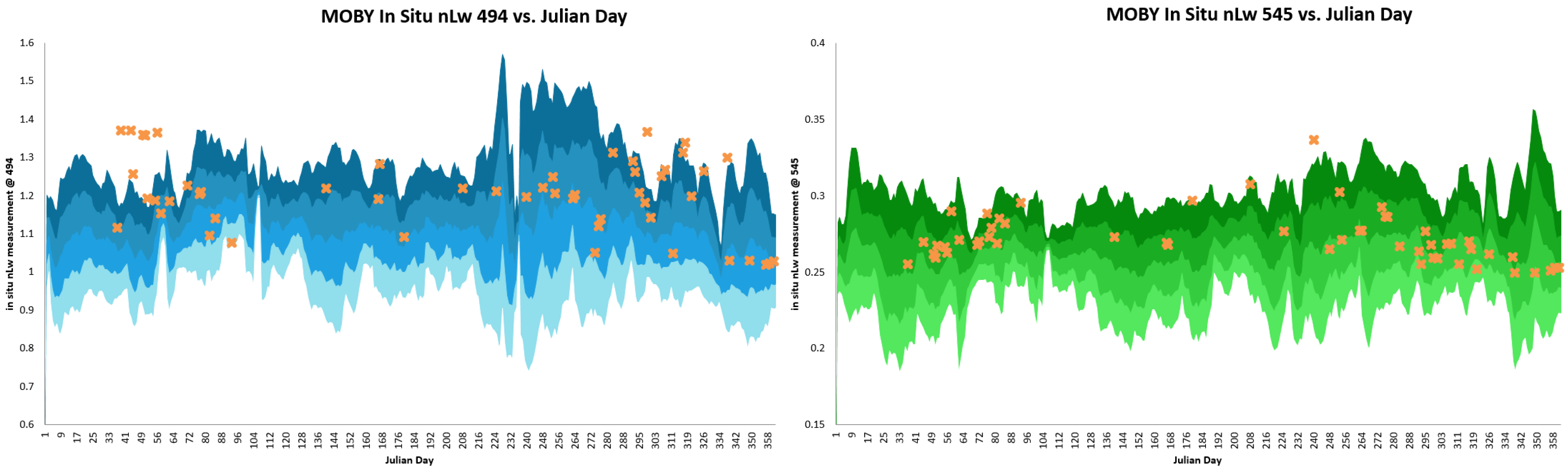
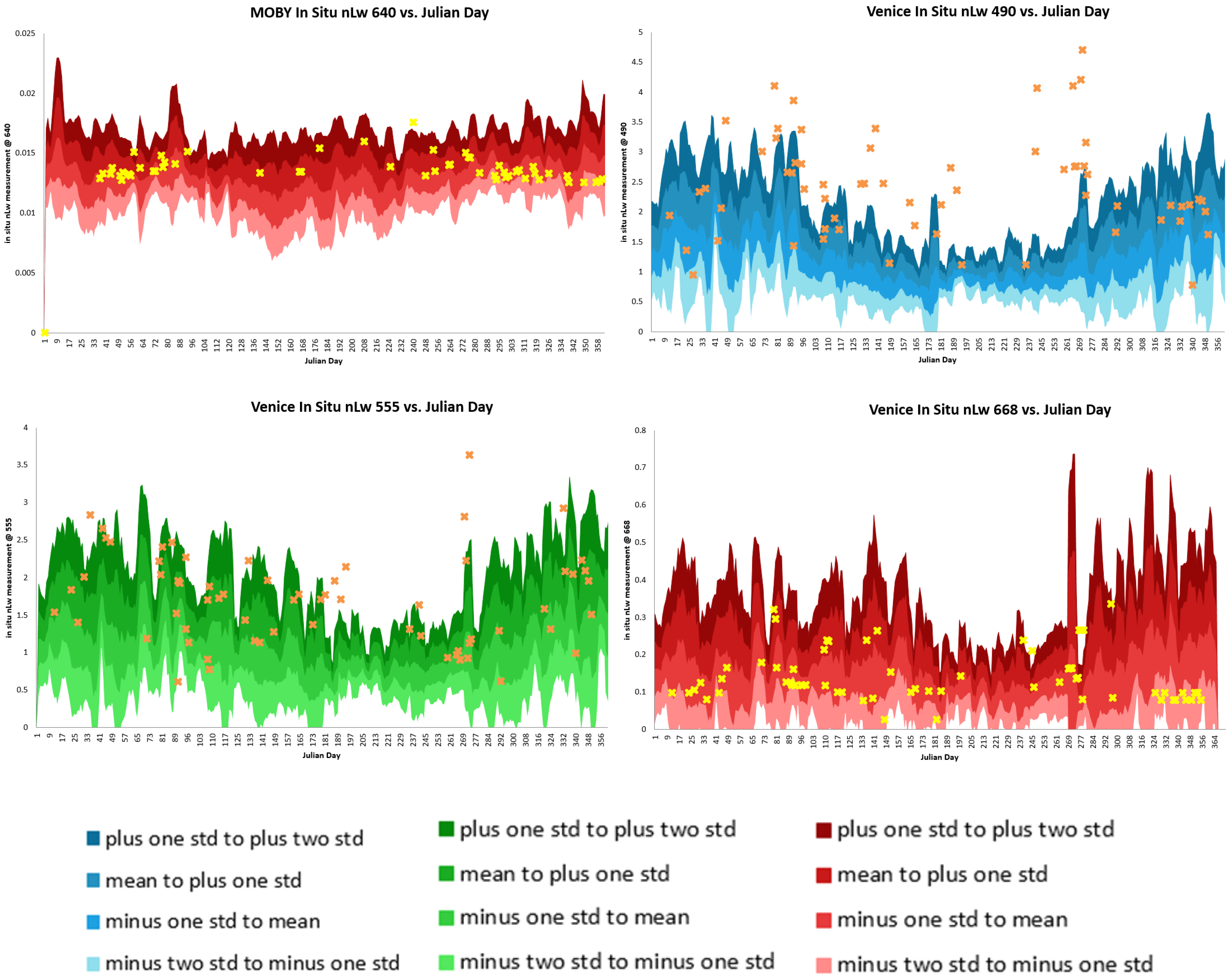
The first study area was the MOBY in situ mooring off the island of Lanai in Hawaii, which records hyperspectral nLw measurements. The second study was the AERONET-OC platform off the coast of Venice, Italy yielding multi-spectral above water nLw measurements. Throughout the remainder of this text, we refer to those two locations as MOBY and Venice. We downloaded historical radiometric and geometric corrected Level 1B SNPP VIIRS data sets from 1 January 2017 through 31 December 2019 for both study sites. We also downloaded historical PlanetScope scenes within the same time period with valid in situ nLw measurements on the same day within a 3 h time period. Level 1B (Scientific Data Records—SDR) VIIRS datasets were downloaded from NOAA’s Comprehensive Large Array-data Stewardship System (CLASS, www.class.noaa.gov). We processed the Level 1B VIIRS datasets, composed of scientific data records (raw radiance + calibration) to Level 3 (fully calibrated, atmospherically corrected, and mapped) using the NRL’s Automated Processing System (APS). APS, which is built on the NASA SeaDAS level 1 to level 2 (l2gen) processing code, is used to ingest multi- and hyperspectral remote sensing data from continuously imaging ocean color sensors. APS produces numerous products of interest to Navy operations, some of which can be used as inputs to bio-optical forecasting models [33]. All VIIRS datasets were processed using the standard Gordon–Wang atmospheric correction routines (Figure 1), utilizing multi-scattering and iterative NIR correction [34].

We used VIIRS historical L1B images at the two study sites to train our atmospheric correction models to predict nLw at the blue, green, and red wavelengths. To begin this process, we extracted Lt, Lr, and nLw from the VIIRS visible bands at cloud and glint-free box domains around the MOBY and AERONET-OC Venice in situ locations (Figure 2). The satellite data were constrained by default to exclude any pixels that had the following quality flags: cloud contamination, high top of atmosphere radiance, land, glint, and atmospheric correction failure. Once the processing algorithms determined if one of these conditions existed, a bad data value was set for that pixel, and no nLw or other derived products were made available. In addition, high satellite angles were excluded. The solar zenith flag was set for pixels above 75 degrees, while the sensor zenith was set for above 60 degrees. The cloud albedo was the default value used for VIIRS processing (0.027) [35,36]. Despite the quality control process, some pixels around cloud edges or haze were still processed, resulting in errors. Additional filtering methods were required and are discussed within this paper.

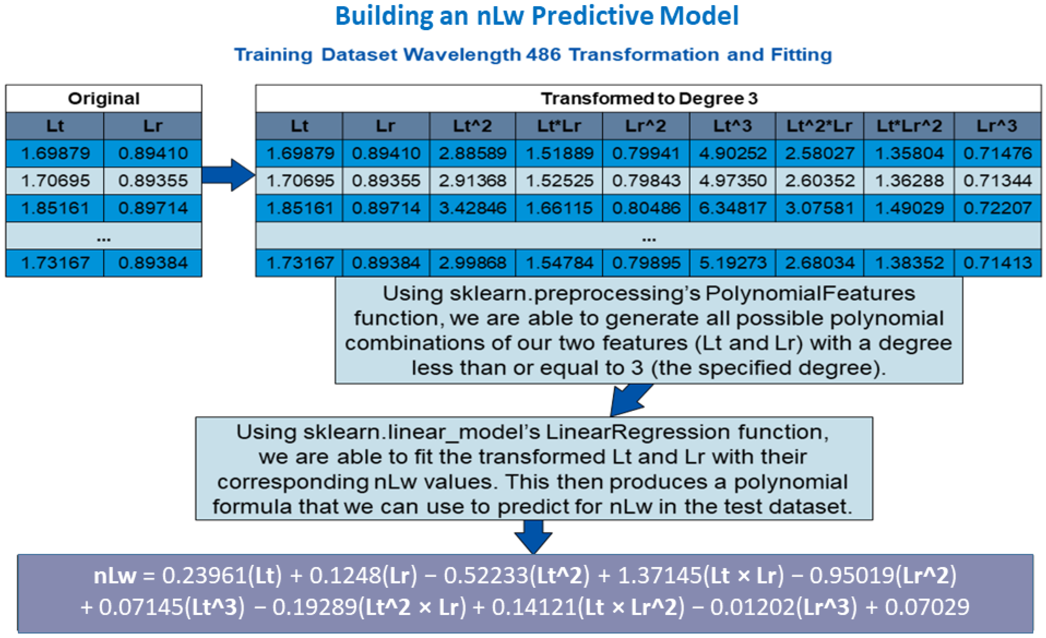
Once we processed and obtained the Lt, Lr, and nLw values used to train our models, we started developing the models for predicting nLw when only Lt and Lr are available. Our efforts focused on obtaining the most correlated answer using the multi-variate regression analysis tools available in the Python scikit-learn toolkit. Scikit-learn (https://scikit-learn.org/stable) is an open-source machine learning library that supports a multitude of solutions that support all aspects of machine learning ranging from data processing to model selection and fitting, evaluation, and post-analysis functions. Attempts to utilize TensorFlow for this effort yielded a performance response that fared no better than scikit-learn, which came with lower overhead and general system requirements, thus leaving our team to focus on the scikit-learn API alone.

The overall methodology used was as follows: (1) data extraction and initial preparation; (2) data cleaning and versioning; (3) neural training; (4) prediction; (5) analysis and results. Each step of the process was designed to be efficient, informative (collating results into easily understood and parsed output), and repeatable. Data extraction and initial preparation focused on marshaling the data from the traditional sensor’s domain of wavelengths and performing initial quality assurance and concatenation of temporal data into a Pandas Data-frame. Data cleansing and versioning focused on applying geospatial minimum/maximum boundaries for each wavelength using the Satellite Validation Navy Tool (SAVANT) in situ data capture, as well as the removal of incomplete records, NaN’s, and similar “bad data” artifacts [37]. With Steps 1 and 2 complete, the neural training could begin.

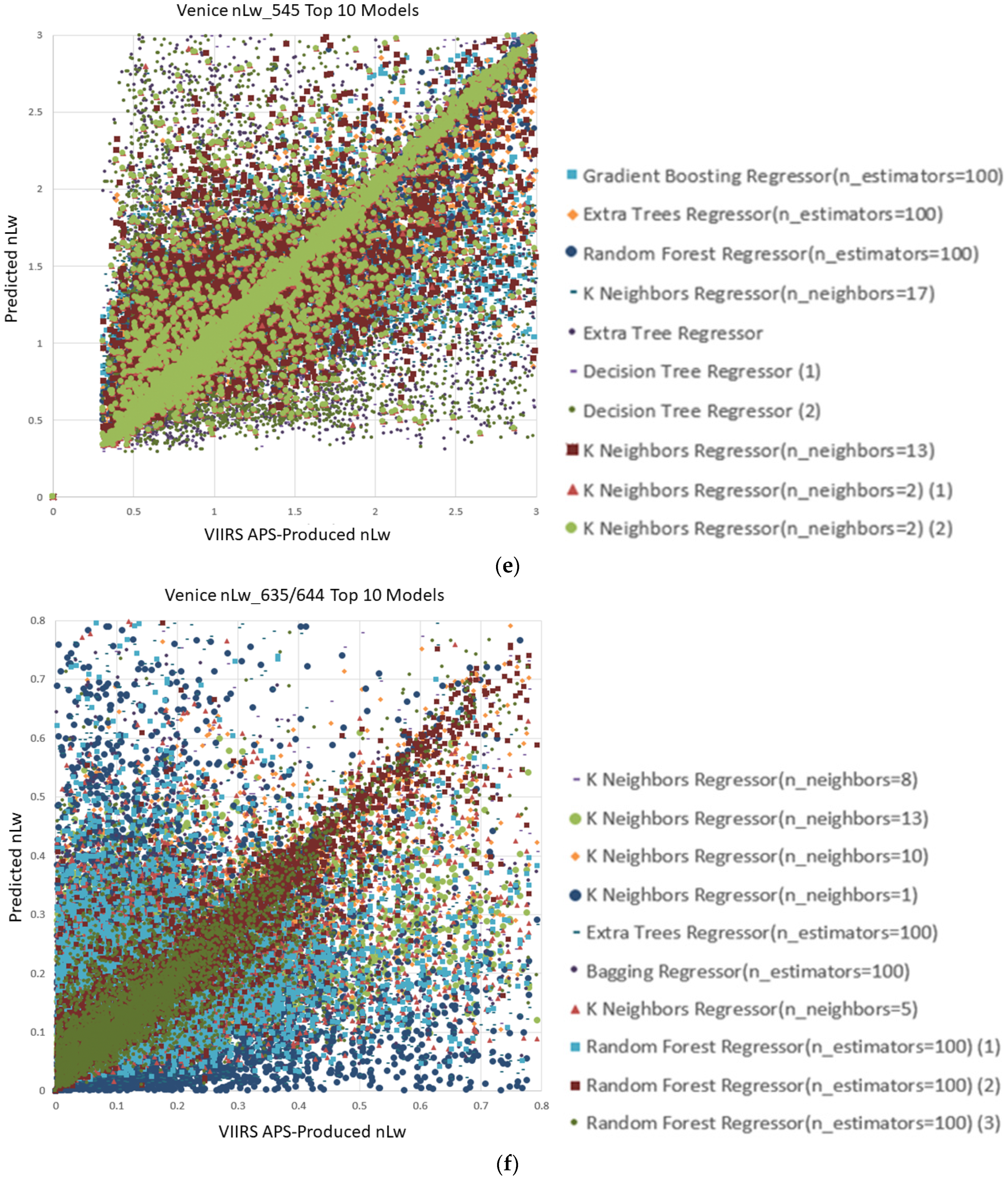
Our solution utilized linear models, support vector machines, nearest neighbors, decision trees, and ensemble methods combined with multiple perturbations of those models when available. Our dependent variable selection of nLw was supported by combinations of “Lt_ λ”, “Lr_λ”, and “(Lt_ λ—Lr_ λ)/Lt_ λ”, for each of the target wavelengths (represented as λ) matching between the PlanetScope nanosatellite domain to the more readily available and operational VIIRS sensor.

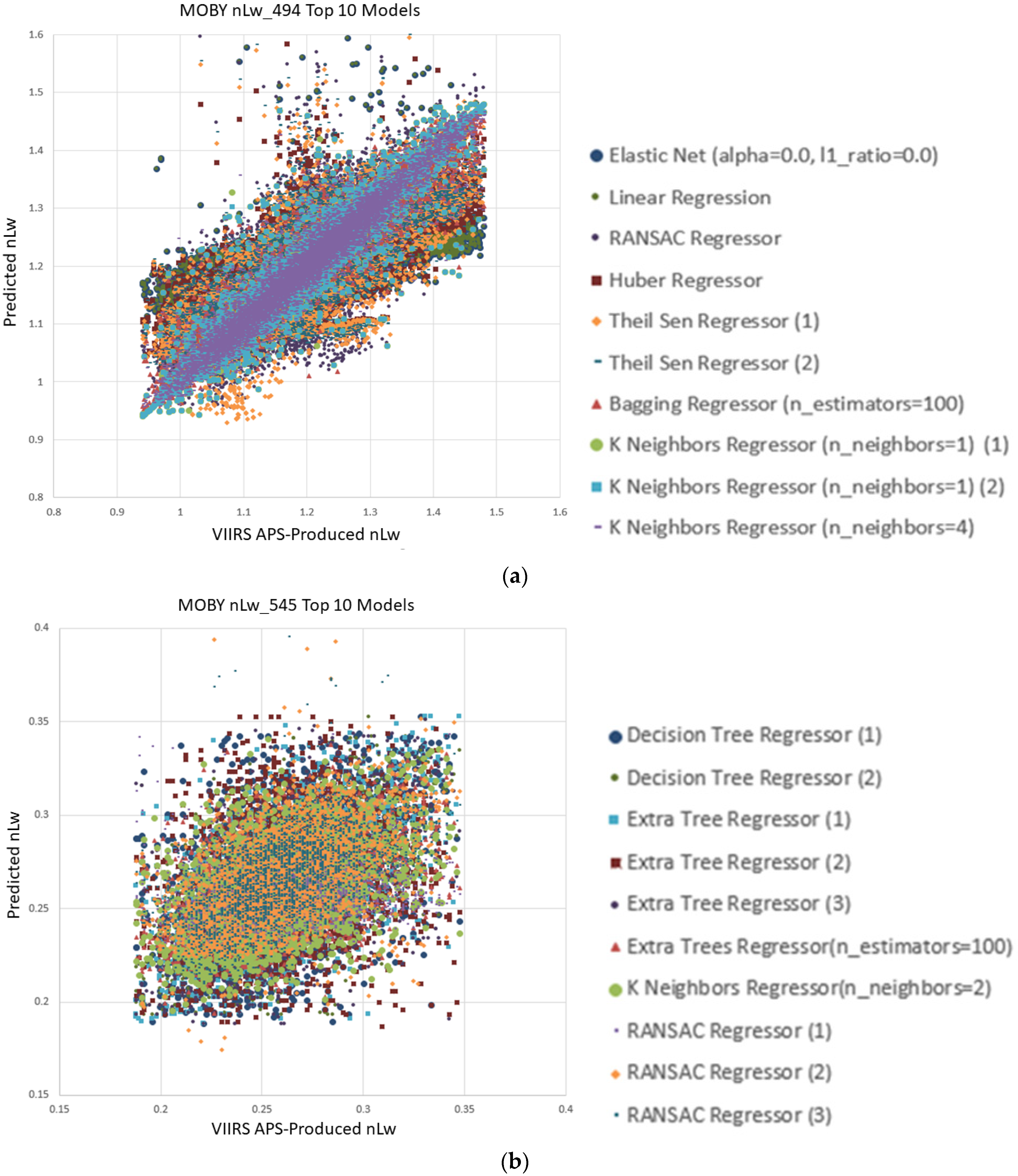
The domain of explicit models utilized in training were as follows: Lasso, Ridge, Elastic Net, Huber Regressor, Lars, Lasso Lars, Passive Aggressive Regressor, RANSAC Regressor, SGC Regressor, Theil Regressor, K Nearest Neighbors Regressor, Decision Tree Regressor, Extra Tree Regressor, SVR, SVMR, Ada Boot Regressor, Bagging Regressor, Random Forest Regressor, and Gradient Boosting Regressor.

Training was performed using an 80/20 train/test split using k-fold cross validation on five splits. The total effort resulted in 188 combinations of the aforementioned models for a total of 4701 total potential neural layers evaluated. This approach allowed for two desired outcomes: (1) each wavelength could potentially have a unique set of data that would not yield the most optimal result given single-use model approaches; (2) by selecting the top-performing models, further refinements to the prediction could be achieved by combining models into a more robust ensemble. This methodology afforded the team the most flexible approach towards potential end-user solutions; however, models were not combined during this analysis. The resulting neural layers selected per region per wavelength were then loaded and applied to the Planet nanosatellite datasets. A NetCDF of original and predicted values was then created for each model, region, and wavelength in question.

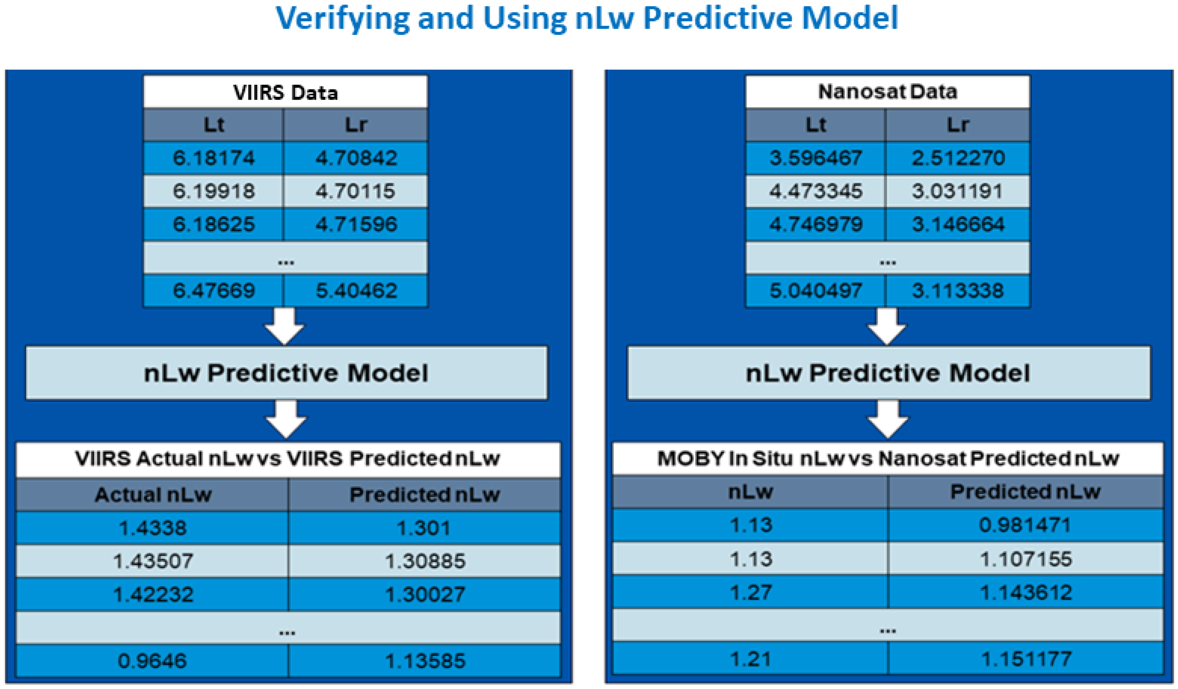
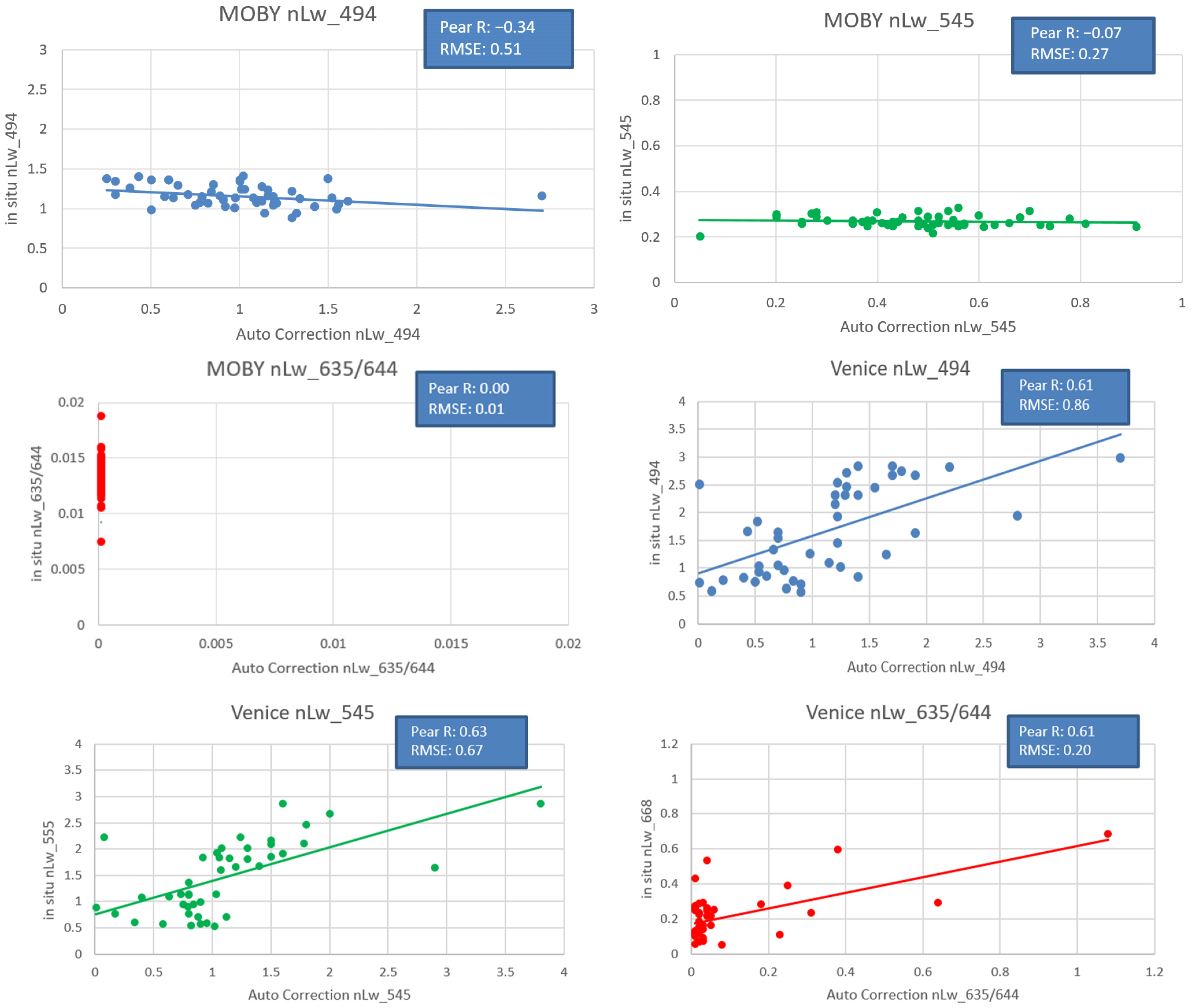
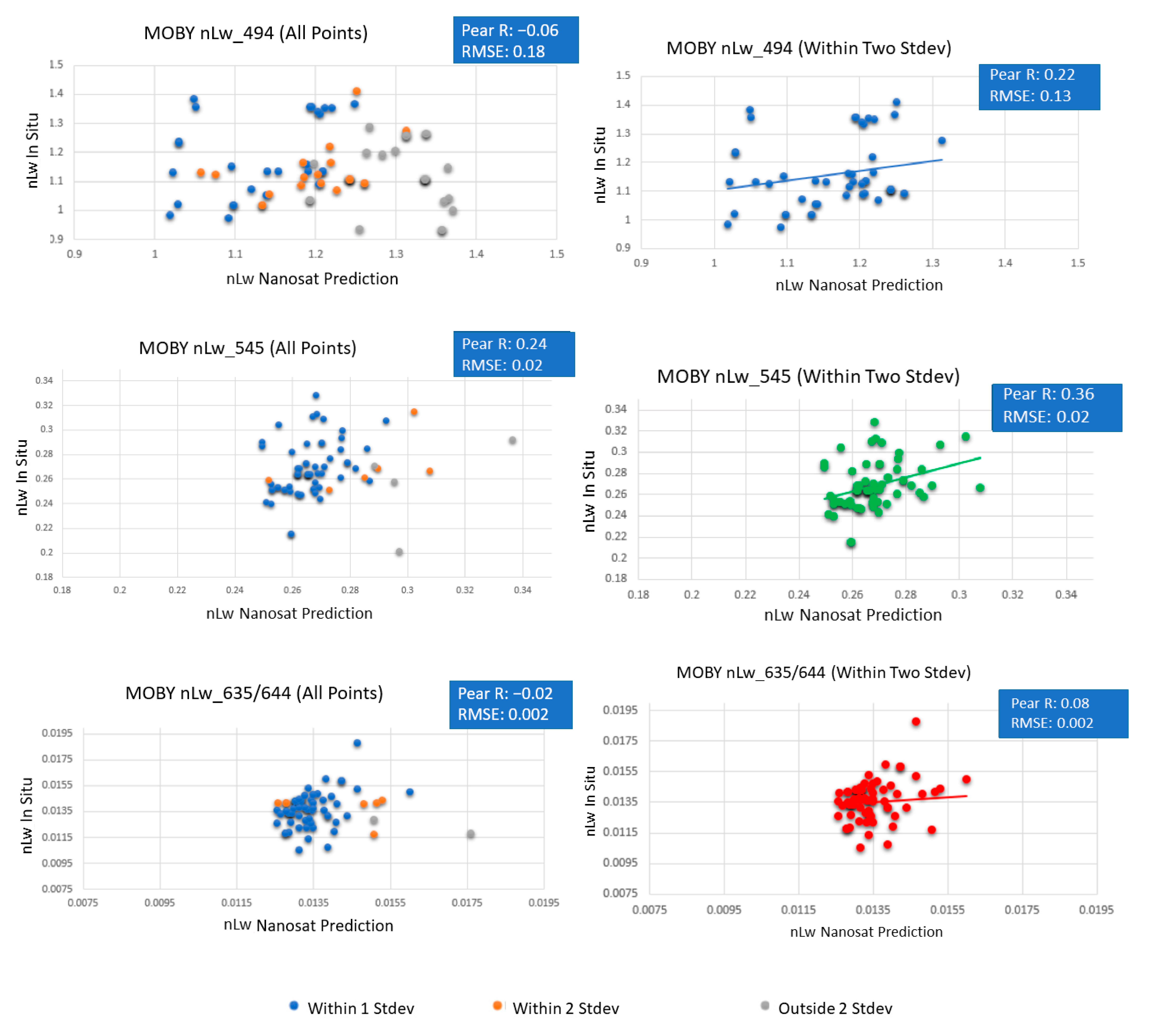
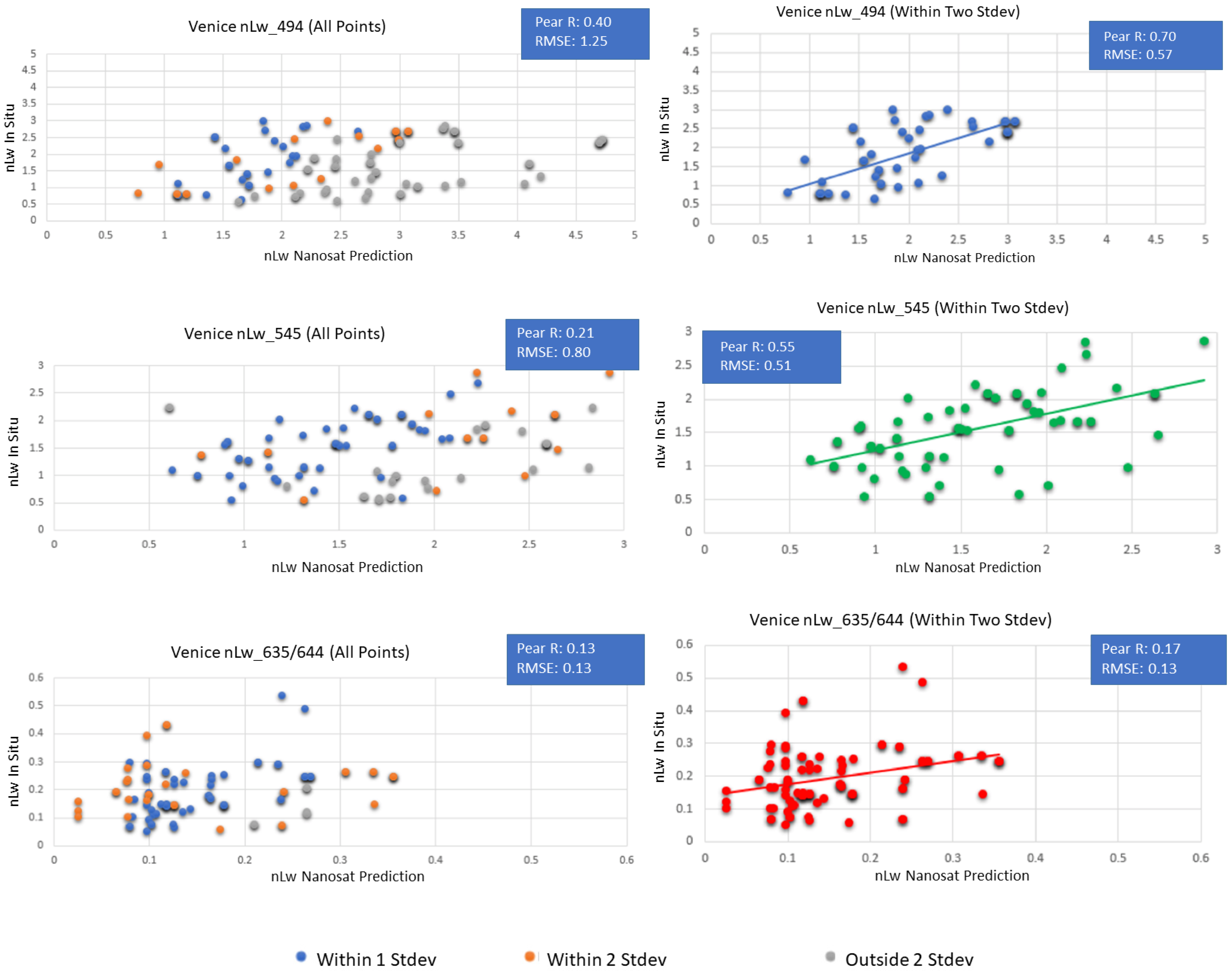
Once the models were established for each visible band to predict nLw for each visible band, our next step was to verify the accuracy of our nLw predictive model by applying it to the 20% of the dataset that was withheld from training. Once we ensured model accuracy of our nLw predictions for VIIRS by comparing predicted VIIRS nLw values to “actual” APS atmospherically corrected nLw values (using the Gordon–Wang standard), we applied our model to the nanosatellite datasets and compared those results to the MOBY and AERONET-OC in situ nLw measurements. Figure 3 depicts an example of a linear regression model created during this study.

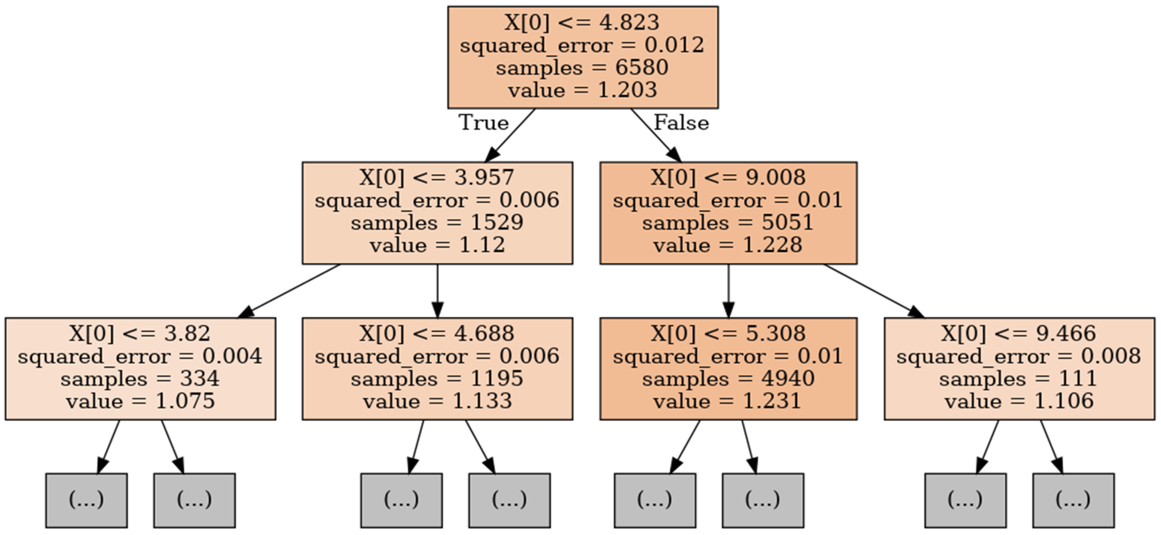
Decision trees are a popular supervised learning method for a variety of reasons. Benefits of decision trees include that they can be used for both regression and classification, they do not require feature scaling, and they are relatively easy to interpret through visualization. The goal is to create a model that predicts the value of a target variable by learning simple decision rules inferred from the data features. A tree can be seen as a piecewise constant approximation. This type of non-parametric supervised algorithm utilizes a binary tree graph to assign a target value for each data sample.

The target values are presented in the tree leaves. To reach the leaf, the sample is propagated through nodes, starting at the root node. In each node a decision is made as to which descendant node it should go. A decision is made based on the selected sample’s features. Decision tree learning is a process of finding the optimal rules in each internal tree node according to the selected metric. In a DecisionTreeRegressor as designed in the scikit-learn API, the value shown in a visual depiction of a subject tree is the value that the tree would predict for a new example falling in that node. If the criterion is mean standard error (MSE), the value is an average measure of the samples in that node. Samples represent the number of sample data points that are used for each leaf of the tree in the decision-making progress. Figure 4 is an example schematic of a decision tree model created during this study.

3. Results

Here we assess the accuracy of two methods for atmospherically correcting small satellite imagery that do not have the desired NIR/SWIR bands required for atmospheric correction. Both methods apply initial atmospheric corrections by removing the Rayleigh radiance contribution (Lr) from Lt at the blue, green, and red Planet channels. Both methods select a group of 11 × 11 neighboring pixels (resulting in 121 possible pixel extractions per nanosatellite scene) centered on the MOBY and Venice locations within the nanosatellite image. These values are averaged to determine the nLw value to match against the in situ nLw value. Additionally, we determined a range of valid nLw values for each wavelength determined by the full range of nLw values observed at the in situ locations from 2014 to 2019.

3.1. Standard Atmospheric Correction Approach

The first method to atmospherically correct Planet’s nanosatellites was the standard approach for operational processing: using Planet’s nanosatellites’ red and NIR bands to automatically select a pair of bounding aerosol models to remove the aerosol contribution from Lt in the visible bands. As expected, this method produced poor matchups when spectral nLw was compared to coincidental in situ nLw measurements at the MOBY location. The mooring at the MOBY location was hyperspectral, so nLw could be convolved to the sensor’s RSR and comparisons could be made at the satellite sensor’s precise center wavelengths. However, the Venice AERONET-OC in situ platform was multi-spectral, so only the closest wavelength could be used in comparisons. This was impactful for the green and red bands, where the closest Venice AERONET-OC wavelengths were 555 nm and 668 nm, respectively.

The results at the Venice AERONET-OC location were considerably better than the open ocean MOBY site, but the Venice AERONET-OC results (Figure 5) did not include scenes where atmospheric correction failed. (Note: nLw_635/644 represents nLw_635 or nLw_644, depending on the nanosatellite flock.) Several scenes could not produce nLw values, and this result skewed the comparisons unless filtering methods were also applied during the model predictions discussed later within this paper. The results shown only encompassed a subset of the entire nanosatellite dataset. However, for the scenes that passed corrections, good correlations and relatively low errors were observed for the blue and green bands at the Venice AERONET-OC location (Figure 5).

As an additional filtering method for our predictive models, we observed the natural variability at the in situ locations by looking at the entire climatological records at these locations. To avoid any potential data gaps, we used 5-day averages centered on the day of interest (e.g., Julian day 2 included Julian days 365, 1, 2, 3, and 4). In the event of a leap year, February 29 measurements were combined with February 28. Since some processed pixels were on cloud edges or consisted of haze that was not flagged during processing, having a climatology to determine if values are realistic could be used to filter erroneous results. We used this information (Figure 6) to constrain realistic nLw model predictions for an accurate evaluation of the results. For the MOBY red in situ values, we focused on nLw_640, rather than having separate plots for both nLw_635 and nLw_644.

3.2. Building Models to Predict nLw

Next, we assessed the second method for atmospherically correcting these datasets. We developed atmospheric correction models from a VIIRS training set and used them to atmospherically correct the nanosatellite data. Our first step for testing the accuracy of the atmospheric correction models was to test against VIIRS imagery outside of the training set. We used VIIRS imagery at or around the MOBY and Venice locations to train and test our atmospheric correction models, using the 80/20 test/train split. We determined the APS atmospherically processed VIIRS imagery outside of our training set to be the “actual” nLw values that we used to evaluate our nLw model predictions. Figure 7 shows the Top 10 (based on RMSE) atmospheric correction model predictive results compared to the real VIIRS values. For each subfigure within Figure 7, the top 10 models used are listed to the right of each plot, with the 10th best model listed first (top) and the best model listed last (bottom). Each color/shape is representative of a single predictive model.

The same atmospheric correction model did not necessarily produce the best results across all wavelengths and for each study area. However, K Neighbors regressors (with varying neighbors and folds) had the most reliable performance, producing the best model three times and having a top-three finish seven times. The Extra Tree and Random Forest regressors also achieved good results.

Table 2. Predictive model performance for various models based on Top 10 finishes as observed in Figure 7a–f. The numbers at the top of this table indicate which rank a model achieved if found within the Top 10 in any results observed within Figure 7a–f.

Predictive Model Name	1	2	3	4	5	6	7	8	9	10
Elastic Net								1		1
Linear Regression									1
RANSAC Regressor	1	1	1				1	1
Huber Regressor	1						1
Theil Sen Regressor			1		2	2
Bagging Regressor		1		1	1	1	1			1
K Neighbors Regressor	3	2	2	2			2	1	3	2
Decision Tree Regressor				1	1				1	1
Extra Tree Regressor		1	1	1	2	3	1	2	1
Random Forest Regressor	1	1	1	1				1
Gradient Boosting Regressor										1

summarizes the results from Figure 7a–f.

After verifying model accuracy by observing good correlation and low errors when applied to VIIRS in the red, green, and blue bands, we applied the best model for each wavelength to the nanosatellite datasets to predict nLw for those bands. For example, the second fold of the K neighbors regressor with two neighbors performed the best for Venice nLw_545 predictions, so that model was used only for that wavelength at that study area. Only the top model for each wavelength/study area was used for the remainder of this assessment.

Once the nanosatellite nLw predictions were made, we compared them to coincidental (same day, within 3 h) MOBY and Venice AERONET-OC in situ nLw measurements to determine accuracy. Figure 8 displays Planet PlanetScope nanosatellite nLw predictions plotted along the MOBY and Venice AERONET-OC in situ nLw climatologies. The nLw predictions that fell outside of two standard deviations from the mean were usually due to scenes and/or pixels that would normally be flagged as contaminated during the standard atmospheric correction process. These scenes coincide with the VIIRS scenes that failed atmospheric corrections during the standard process (Figure 5) and were excluded from the results. Our prediction code that applies the models to the Planet images did not currently filter these pixels like the standard atmospheric correction code within APS, but future efforts aim to combine these approaches. Figure 8 overlays the PlanetScope nLw model predictions onto the climatological datasets displayed in Figure 6.

For the MOBY location, the majority of the blue (71%), green (92%), and red (96%) nanosatellite predictions fall within two standard deviations of the in situ mean for that corresponding day. There are some seasonal biases for the nLw_494 predictions, where the values tend to be elevated in the winter months. For the Venice location, the majority of the green (71%) and red (95%) nanosatellite nLw predictions fall within two standard deviations of the in situ mean for that corresponding day, but the nLw blue (49%; 494 nm nanosatellite; 490 nm in situ) predictions are routinely overestimated, especially in the non-winter months. This is the opposite bias we observed at the MOBY location, potentially indicating that a secondary correction can be applied to these datasets to adjust the nLw values more towards observations.

Figure 9 and Figure 10 plot the nLw model predictions vs. in situ nLw values for both the MOBY and Venice AERONET-OC study areas. Matchups that likely fall outside of reality (beyond two standard deviations from the mean), mostly due to pixel contamination that is currently unfiltered, can be filtered from the final nLw predictions. The nanosatellite nLw predictions at the MOBY site had higher Pearson R correlation coefficients in the blue (0.22) and green (0.36) than in the red (0.08). A large factor in the inconsistencies observed between the predicted nanosatellite nLw values and the in situ nLw values for the red band is that the VIIRS training model is centered at 671 nm, while the Planet nanosatellites are centered at 635 and 644 nm, depending on which flock is being analyzed. This is a very large difference in center spectral wavelength, which has a large influence on predicted nLw. The nLw in red is typically higher at the 635 and 644 nm wavelengths than it is at 671 nm. This, combined with the fact that MOBY resides in a deep blue open ocean water location with relatively little red signal led to the inconsistent results. Despite not having strong correlations, the RMSE for the blue, green, and red nanosatellite nLw predictions is low compared to using the red and NIR bands for atmospheric correction, as seen in Figure 5.

The nanosatellite nLw predictions at the Venice site had larger correlation coefficients in the blue (0.70) and green (0.55) bands when compared to the results at MOBY. The correlation in the red (0.17) is indicative of a positive trend and is larger than the red matchup at the MOBY site. The RMSE values in the blue (0.57), green (0.51), and red (0.13) were low and were reduced where outliers were filtered.

For the same nanosatellite dataset illustrated in Figure 9 and Figure 10 (within two standard deviations only), we processed those scenes through the ACOLITE software package. The ACOLITE software package atmospherically corrected the PlanetScope nanosatellite imagery by using dark spectrum fitting (DSF) and produced remote sensing reflectance (Rrs) for the blue, green, and red bands. This method worked well in coastal waters but overestimated Rrs in the visible bands at the deep blue water, open-ocean MOBY in situ location. We converted the Rrs values to nLw using the equation nLw = Rrs * F0, where F0 is the hyperspectral exo-atmospheric solar irradiance (mW/(cm²um)), convolved to the PlanetScope spectral relative spectral response functions [35].

Table 3. PlanetScope series identifiers, center wavelengths based on relative spectral response functions, and F0 constants for each wavelength.

Planet Series	Wavelength	F0
“0C” and “0D”	(490, 545, 649, 820)	(195,46, 183.82, 163.57, 108.21)
“0E”	(494, 545, 644, 824)	(189.05, 181.07, 160.77, 108.27)
“10” and “0F”	(494, 545, 635, 819)	(192.29, 182.73, 163.16, 108.74)

displays these F0 coefficients, along with their respective Planet series.

After converting Rrs to nLw, we compared the results to the MOBY and AERONET-OC in situ nLw values in the same manner as we did for our previous comparisons. ACOLITE lists slightly different center wavelengths for each visible band, so we referred to each visible band simply as blue, green, and red in this analysis (Figure 11).

Our nLw predictions at the MOBY in situ site consistently outperformed the ACOLITE software package, which was to be expected since ACOLITE’s dark spectrum fitting is not built for open ocean atmospheric correction. For the coastal Venice in situ location, our predicted nLw values had a significantly smaller RMSE than ACOLITE for the blue, green, and red wavelengths. However, ACOLITE had a stronger correlation in the green and red bands.

Table 4. Summary containing nLw correlation (Pearson R) and error (RMSE) for MOBY and Venice standard, model prediction, and ACOLITE atmospheric corrections. The best results per wavelength are highlighted.

MOBY Pearson R Correlation
	Standard	Model Prediction	ACOLITE
nLw_Blue	−0.34	0.22	0.02
nLw_Green	−0.07	0.36	0.33
nLw_Red	0.00	0.08	−0.31
Venice Pearson R Correlation
	Standard	Model Prediction	ACOLITE
nLw_Blue	0.61	0.70	0.58
nLw_Green	0.63	0.55	0.62
nLw_Red	0.61	0.17	0.37
MOBY RMSE
	Standard	Model Prediction	ACOLITE
nLw_Blue	0.51	0.13	0.81
nLw_Green	0.27	0.02	1.02
nLw_Red	0.01	0.00	0.34
Venice RMSE
	Standard	Model Prediction	ACOLITE
nLw_Blue	0.86	0.58	1.00
nLw_Green	0.67	0.51	0.84
nLw_Red	0.20	0.13	0.56

details a summary of all atmospheric correction methods described throughout this text. The best performance at each location (MOBY and Venice), for each wavelength (blue, green, and red), for each statistical metric (Pearson R and RMSE) is highlighted. Overall, our model predictions have the best correlation for each wavelength at MOBY and for the blue wavelength at Venice. Our model predictions have the best RMSE for each wavelength at MOBY and Venice, outperforming any automated correction that could be achieved using the Red/NIR combination of bands, as well as the DSF implemented with ACOLITE.

4. Discussion

Here we performed two methods for automating atmospheric correction on data obtained from Planet’s nanosatellites, which do not possess wavelength combinations required for the standard Gordon and Wang atmospheric correction process. Aside from the DSF method used by ACOLITE and using the red band in combination with the NIR band, no accurate method for automated atmospheric correction of these types of satellite sources currently exists. The best choice for our first training/testing location was the area covering MOBY, a buoy that collects hyperspectral in situ nLw measurements. We developed ML-based atmospheric correction models from VIIRS coincident climatological datasets to predict nLw when only Lt and Lr were available. We observed encouraging results, therefore demonstrating that models can be developed from coincident ocean color satellite imagery and be used to atmospherically correct these unconventional satellite sources. This approach was conducted in open ocean waters as well as a more turbid, coastal domain that exhibits faster-changing biology. For the open-ocean observations (MOBY), our approach was shown to improve correlation and RMSE for all wavelengths compared to ACOLITE and using the red/NIR combination for automated atmospheric correction. For the coastal observations (Venice), our approach was shown to improve RMSE for all wavelengths, but our approach had a stronger correlation in only one of the three wavelengths (blue).

Factors not included in this study will be included in future efforts to improve accuracy in training the models to atmospherically correct nanosatellite images. Satellite and solar angles were not accounted for within this study. For example, the VIIRS satellite angles were not as close to nadir as the nanosatellites, which had an impact on Lt and Lr, and subsequently, nLw. Signal-to-noise Ratio (SNR) is also a concern. Planet’s nanosatellites no longer publish the SNR for their nanosatellites, but it is very likely smaller than that of a sensor such as VIIRS. This can lead to uncertainties, especially in the red signal at a domain such as MOBY, where most, if not all, of Lt is noise. Additionally, Planet nanosatellites’ broader wavelengths produce an extra layer of uncertainties within a single wavelength’s Lt. Another factor to consider is how sun glint contamination can require additional filtering methods (beyond what is performed for more coarse spatial resolution sensors) due to Planet’s nanosatellites’ high spatial resolution

Since this project focuses on using data from the 150+ PlanetScope nanosatellites, vicarious calibration of these individual sensors will be a priority moving forward to improve spectral shape and reduce uncertainty between the satellite-derived and in situ nLw values. Even though PlanetScope’s nanosatellites are well calibrated prior to launch, most Earth-orbiting sensors require on-orbit calibration adjustments due to sensor drift and/or degradation, and it will be necessary to apply our own vicarious calibration routines. Traditionally, earth-observing and orbiting sensors are vicariously calibrated using in situ data from sensors such as MOBY and the AERONET-OC. The vicarious calibration process adjusts the prelaunch laboratory calibration to improve the accuracy of the actual in-orbit measurement of the water leaving radiances. During this process, the vicariously calibrated gain set is multiplied by an individual sensor’s spectral Lt values so that the derived spectral nLw values are more accurate.

In summary, ML-based approaches were tested using a calibrated and dedicated ocean color sensor to develop models that derive nLw from Lr and Lt input variables. We observed potential in using this methodology as a means to automatically atmospherically correct ocean color satellite sources that do not possess the wavelengths required by existing, traditional methodologies.

References

1. Marta, S. Planet Imagery Product Specifications; Planet Labs: San Francisco, CA, USA, 2018; p. 91. [Google Scholar]
2. Aldeghi, A.; Carn, S.; Escobar-Wolf, R.; Groppelli, G. Volcano Monitoring from Space Using High-Cadence Planet CubeSat Images Applied to Fuego Volcano, Guatemala. Remote Sens. 2019, 11, 2151. [Google Scholar] [CrossRef] [Green Version]
3. Houborg, R.; McCabe, M.F. High-Resolution NDVI from Planet’s Constellation of Earth Observing Nano-Satellites: A New Data Source for Precision Agriculture. Remote Sens. 2016, 8, 768. [Google Scholar] [CrossRef] [Green Version]
4. Shi, Y.; Huang, W.; Ye, H.; Ruan, C.; Xing, N.; Geng, Y.; Dong, Y.; Peng, D. Partial least square discriminant analysis based on normalized two-stage vegetation indices for mapping damage from rice diseases using PlanetScope datasets. Sensors 2018, 18, 1901. [Google Scholar] [CrossRef] [PubMed] [Green Version]
5. Aragon, B.; Houborg, R.; Tu, K.; Fisher, J.B.; McCabe, M. CubeSats Enable High Spatiotemporal Retrievals of Crop-Water Use for Precision Agriculture. Remote Sens. 2018, 10, 1867. [Google Scholar] [CrossRef] [Green Version]
6. Breunig, F.M.; Galvão, L.S.; Dalagnol, R.; Dauve, C.E.; Parraga, A.; Santi, A.L.; Della Flora, D.P.; Chen, S. Delineation of management zones in agricultural fields using cover–crop biomass estimates from PlanetScope data. Int. J. Appl. Earth Obs. Geoinf. 2020, 85, 102004. [Google Scholar] [CrossRef]
7. Cooley, S.W.; Smith, L.C.; Ryan, J.C.; Pitcher, L.H.; Pavelsky, T.M. Arctic-Boreal Lake Dynamics Revealed Using CubeSat Imagery. Geophys. Res. Lett. 2019, 46, 2111–2120. [Google Scholar] [CrossRef]
8. Ghuffar, S. DEM generation from multi satellite PlanetScope imagery. Remote Sens. 2018, 10, 1462. [Google Scholar] [CrossRef] [Green Version]
9. Schaeffer, B.A.; Whitman, P.; Conmy, R.; Salls, W.; Coffer, M.; Graybill, D.; Lebrasse, M.C. Potential for commercial PlanetScope satellites in oil response monitoring. Mar. Pollut. Bull. 2022, 183, 114077. [Google Scholar] [CrossRef]
10. Liu, H.; Dahlgren, R.A.; Larsen, R.E.; Devine, S.M.; Roche, L.M.; O’ Geen, A.T.; Wong, A.J.Y.; Covello, S.; Jin, Y. Estimating Rangeland Forage Production Using Remote Sensing Data from a Small Unmanned Aerial System (sUAS) and PlanetScope Satellite. Remote Sens. 2019, 11, 595. [Google Scholar] [CrossRef] [Green Version]
11. Kameche, M.; Benzeniar, H.; Benbouzid, A.B.; Amri, R.; Bouanani, N. Disaster monitoring constellation using nanosatellites. J. Aerosp. Technol. Manag. 2014, 6, 93–100. [Google Scholar] [CrossRef] [Green Version]
12. Asner, G.P.; Martin, R.E.; Mascaro, J. Coral reef atoll assessment in the South China Sea using Planet Dove satellites. Remote Sens. Ecol. Conserv. 2017, 3, 57–65. [Google Scholar] [CrossRef]
13. Cooley, S.W.; Smith, L.C.; Stepan, L.; Mascaro, J. Tracking Dynamic Northern Surface Water Changes with High-Frequency Planet CubeSat Imagery. Remote Sens. 2017, 9, 1306. [Google Scholar] [CrossRef] [Green Version]
14. Vanhellemont, Q. Daily metre-scale mapping of water turbidity using CubeSat imagery. Opt. Express 2019, 27, A1372–A1399. [Google Scholar] [CrossRef]
15. Hang, N.T.; Hoa, N.T.; Son, T.P.H.; Nguyen-Ngoc, L. Vegetation Biomass of Sargassum Meadows in An Chan Coastal Waters, Phu Yen Province, Vietnam Derived from PlanetScope Image. J. Environ. Sci. Eng. B 2019, 8, 81–92. [Google Scholar]
16. Kääb, A.; Altena, B.; Mascaro, J. River-ice and water velocities using the Planet optical cubesat constellation. Hydrol. Earth Syst. Sci. 2019, 23, 4233–4247. [Google Scholar] [CrossRef] [Green Version]
17. Poursanidis, D.; Traganos, D.; Chrysoulakis, N.; Reinartz, P. Cubesats Allow High Spatiotemporal Estimates of Satellite-Derived Bathymetry. Remote Sens. 2019, 11, 1299. [Google Scholar] [CrossRef] [Green Version]
18. Wicaksono, P.; Lazuardi, W. Assessment of PlanetScope images for benthic habitat and seagrass species mapping in a complex optically shallow water environment. Int. J. Remote Sens. 2018, 39, 5739–5765. [Google Scholar] [CrossRef]
19. Barschke, M.F.; Bartholomäus, J.; Gordon, K.; Lehmann, M.; Brieß, K. The TUBIN nanosatellite mission for wildfire detection in thermal infrared. CEAS Space J. 2017, 9, 183–194. [Google Scholar] [CrossRef]
20. Antonini, K.; Langer, M.; Farid, A.; Walter, U. SWEET CubeSat—Water detection and water quality monitoring for the 21st century. Acta Astronaut. 2017, 140, 10–17. [Google Scholar] [CrossRef]
21. Mhangara, P.; Mapurisa, W.; Mudau, N. Image Interpretability of nSight-1 Nanosatellite Imagery for Remote Sensing Applications. Aerospace 2020, 7, 19. [Google Scholar] [CrossRef] [Green Version]
22. Piro, A.; Casella, D.; Ciolo, L.D.; Pinori, S.; Cappelleti, C.; Battistini, S.; Graziani, F. HYBRIS: Analysis and Design of a Hyper-Spectral CubeSat Mission for Multiple Remote Sensing Applications and Earth Observation Synergies. In Proceedings of the The 4S Symposium 2018, Sorrento, Italy, 28 May–1 June 2018. [Google Scholar]
23. Wu, S.; Zhao, T.; Gao, Y.; Cheng, X. Design and implementation of a Cube satellite mission for Antarctic glacier and sea ice observation. Acta Astronaut. 2017, 139, 313–320. [Google Scholar] [CrossRef]
24. Groom, S.; Sathyendranath, S.; Ban, Y.; Bernard, S.; Brewin, R.; Brotas, V.; Brockmann, C.; Chauhan, P.; Choi, J.-K.; Chuprin, A.; et al. Satellite Ocean Colour: Current Status and Future Perspective. Front. Mar. Sci. 2019, 6, 1–30. [Google Scholar] [CrossRef] [Green Version]
25. Maciel, D.A.; Novo, E.M.L.D.M.; Barbosa, C.C.F.; Martins, V.S.; Flores Júnior, R.; Oliveira, A.H.; Sander De Carvalho, L.A.; Lobo, F.D.L. Evaluating the potential of CubeSats for remote sensing reflectance retrieval over inland waters. Int. J. Remote Sens. 2020, 41, 2807–2817. [Google Scholar] [CrossRef]
26. Vanhellemont, Q. Adaptation of the dark spectrum fitting atmospheric correction for aquatic applications of the Landsat and Sentinel-2 archives. Remote Sens. Environ. 2019, 225, 175–192. [Google Scholar] [CrossRef]
27. Vanhellemont, Q. Sensitivity analysis of the dark spectrum fitting atmospheric correction for metre- and decametre-scale satellite imagery using autonomous hyperspectral radiometry. Opt. Express 2020, 28, 29948–29965. [Google Scholar] [CrossRef]
28. Gordon, H.R.; Wang, M. Retrieval of water leaving radiance and aerosol optical thickness over the oceans with SeaWiFS: A preliminary algorithm. Appl. Opt. 1994, 33, 443–452. [Google Scholar] [CrossRef]
29. Wang, M.; Gordon, H.R. A simple, moderately accurate, atmospheric correction algorithm for SeaWiFS. Remote Sens. Environ. 1994, 50, 231–239. [Google Scholar] [CrossRef]
30. Ahmad, Z.; Franz, B.A.; McClain, C.R.; Kwiatkowska, E.J.; Werdell, J.; Shettle, E.P.; Holben, B.N. New aerosol models for the retrieval of aerosol optical thickness and normalized water-leaving radiances from the SeaWiFS and MODIS sensors over coastal regions and open oceans. Appl. Opt. 2010, 49, 5545–5560. [Google Scholar] [CrossRef]
31. McCarthy, S.C.; Gould, R.W.; Richman, J.; Kearney, C.; Lawson, A. Impact of Aerosol Model Selection on Water-Leaving Radiance Retrievals from Satellite Ocean Color Imagery. Remote Sens. 2012, 4, 3638–3665. [Google Scholar] [CrossRef] [Green Version]
32. Lewis, M.D.; Gould, R.W.; Arnone, R.A.; Lyon, P.E.; Martinolich, P.M.; Vaughan, R.; Lawson, A.; Scardino, T.; Hou, W.; Snyder, W.; et al. The Hyperspectral Imager for the Coastal Ocean (HICO): Sensor and data processing overview. In Proceedings of the OCEANS 2009, Biloxi, MI, USA, 26–29 October 2009; pp. 1–9. [Google Scholar]
33. Jolliff, J.K.; Ladner, S.; Crout, R.; Lyon, P.E.; Matulewski, K.; Arnone, R.A.; Lewis, D. Forecasting the Ocean’s Optical Environment Using the BioCast System. Oceanography 2014, 27, 68–79. [Google Scholar] [CrossRef] [Green Version]
34. Ladner, S.; Crout, L.R.; Lawson, A.; Wood, C.; Martinolich, P.M.; Bowers, J. Validation Test Report for the Automated Optical Processing System (AOPS) Version 19; NRL/MR/7331-19-9959; Defense Technical Information Center: Fort Belvoir, VA, USA, 2020; p. 64.
35. Bailey, S.W.; Werdell, P.J. A multi-sensor approach for the on-orbit validation of ocean color satellite data products. Remote Sens. Environ. 2006, 102, 12–23. [Google Scholar] [CrossRef]
36. Wang, M.; Son, S.; Shi, W. Evaluation of MODIS SWIR and NIR-SWIR atmospheric correction algorithms using SeaBASS data. Remote Sens. Environ. 2009, 113, 635–644. [Google Scholar] [CrossRef]
37. Lawson, A.; Bowers, J.; Ladner, S.; Crout, R.; Wood, C.; Arnone, R.; Martinolich, P.; Lewis, D. Analyzing Satellite Ocean Color Match-Up Protocols Using the Satellite Validation Navy Tool (SAVANT) at MOBY and Two AERONET-OC Sites. Remote Sens. 2021, 13, 2673. [Google Scholar] [CrossRef]
Figure 1. Standard atmospheric correction process implemented within NRL’s APS, built upon NASA’s SeaDAS processing code.
Jmse 11 00660 g001
Figure 2. Left Image: VIIRS True Color Image, 16 March 2019. The red box is centered around the MOBY hyperspectral nLw in situ mooring, located off the Hawaiian island of Lanai. Right Image: VIIRS True Color Image, 28 February 2021. The red box is centered around the AERONET-OC multispectral nLw in situ platform, located off the coast of Venice, Italy. All valid pixels within the red box were used for training the atmospheric correction models to be used for atmospherically correcting the nanosatellite imagery.
Jmse 11 00660 g002
Figure 3. Complete methodology for building and validating a linear regression nLw predictive model at wavelength 486 nm from VIIRS training datasets at the MOBY nLw in situ mooring.
Jmse 11 00660 g003aJmse 11 00660 g003b
Figure 4. Example decision tree regressor nLw predictive model at 486 nm, built from VIIRS training datasets at the MOBY nLw in situ mooring.
Jmse 11 00660 g004
Figure 5. Gordon–Wang automated atmospheric correction using Planet PlanetScope’s duplicated red band and NIR band. Top left: MOBY nLw_494. Top right: MOBY nLw_545. Middle left: MOBY nLw_635/644. Middle right: Venice nLw_494. Bottom left: Venice nLw_545. Bottom right: Venice nLw_635/644.
Jmse 11 00660 g005
Figure 6. MOBY and Venice AERONET-OC in situ nLw climatologies. Top left: MOBY in situ nLw_494. Top right: MOBY in situ nLw_545. Middle left: MOBY in situ nLw_640. Middle right: Venice AERONET-OC in situ nLw_490. Bottom left: Venice AERONET-OC in situ nLw_555. Bottom right: Venice AERONET-OC in situ nLw_668.
Jmse 11 00660 g006
Figure 7. (a). VIIRS top 10 nLw predictive models compared to the real (APS-processed) nLw_494 at the MOBY study area. (b). VIIRS top 10 nLw predictive models compared to the real (APS-processed) nLw_545 at the MOBY study area. (c). VIIRS top 10 nLw predictive models compared to the real (APS-processed) nLw_636/644 at the MOBY study area. (d). VIIRS top 10 nLw predictive models compared to the real (APS-processed) nLw_494 at the Venice study area. (e). VIIRS top 10 nLw predictive models compared to the real (APS-processed) nLw_545 at the Venice study area. (f). VIIRS top 10 nLw predictive models compared to the real (APS-processed) nLw_635/644 at the Venice study area.
Jmse 11 00660 g007aJmse 11 00660 g007bJmse 11 00660 g007c
Figure 8. MOBY and Venice AERONET-OC in situ nLw climatologies with Planet nanosatellite nLw predictions. Top left: MOBY in situ nLw_494. Top right: MOBY in situ nLw_545. Middle left: MOBY in situ nLw_635/644. Middle right: Venice AERONET-OC in situ nLw_490. Bottom left: Venice AERONET-OC in situ nLw_555. Bottom right: Venice AERONET-OC in situ nLw_668. The orange ‘x’ indicates a nanosatellite nLw predicted value.
Jmse 11 00660 g008aJmse 11 00660 g008b
Figure 9. Planet PlanetScope predicted nLw vs. MOBY in situ nLw. Top left: nLw_494 unfiltered. Top right: nLw_494 filtered. Middle left: nLw_545 unfiltered. Middle right: nLw_545 filtered. Lower left: nLw_635/644 unfiltered. Lower right: nLw_635/644 filtered.
Jmse 11 00660 g009
Figure 10. Planet PlanetScope predicted nLw vs. Venice AERONET-OC in situ nLw. Top left: nLw_494 unfiltered. Top right: nLw_494 filtered. Middle left: nLw_545 unfiltered. Middle right: nLw_545 filtered. Lower left: nLw_635/644 unfiltered. Lower right: nLw_635/644 filtered.
Jmse 11 00660 g010
Figure 11. Planet model predicted nLw and ACOLITE nLw compared to MOBY and Venice AERONET-OC in situ nLw. Top left: MOBY blue nLw. Top right: MOBY green nLw. Middle left: MOBY red nLw. Middle right: Venice AERONET-OC blue nLw. Lower left: Venice AERONET-OC green nLw. Lower right: Venice AERONET-OC red nLw.
Jmse 11 00660 g011aJmse 11 00660 g011b