
Neural Network, Nonlinear-Fitting, Sliding Mode, Event-Triggered Control under Abnormal Input for Port Artificial Intelligence Transportation Robots

Abstract
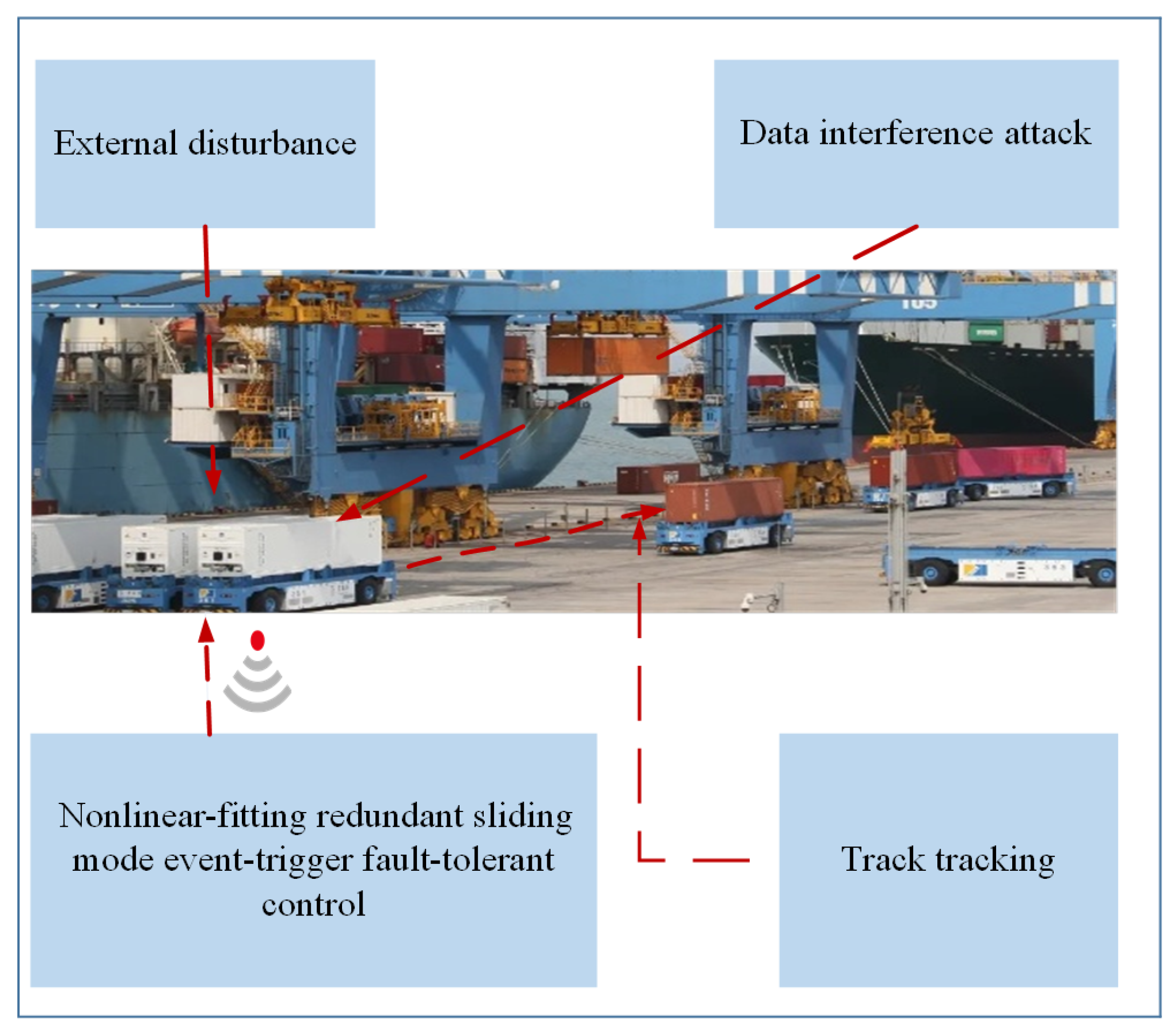
:1. Introduction
2. Model and Preliminaries
2.1. Artificial Intelligence Transportation Robot Model
2.2. Mathematical Model of Abnormal Control
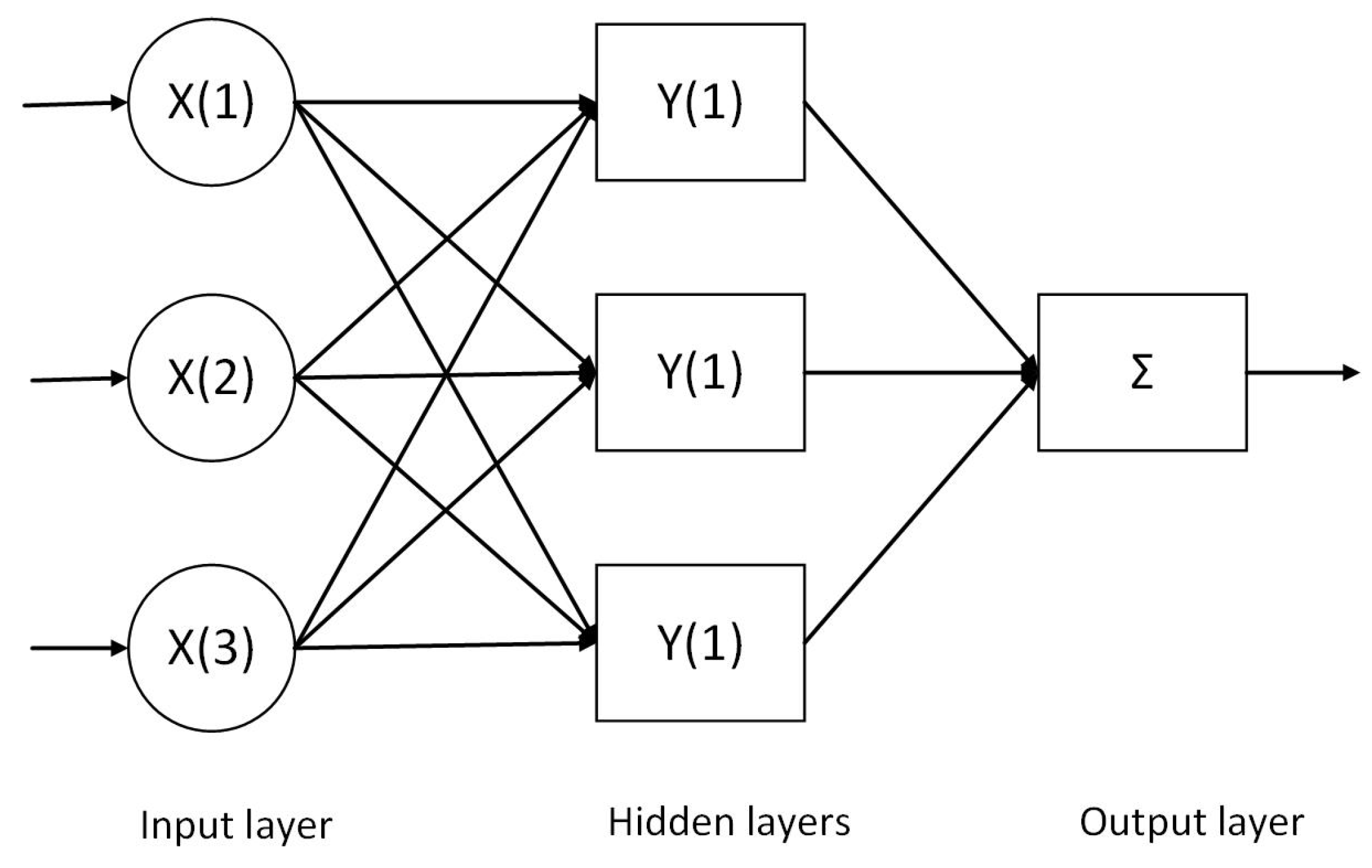
2.3. RBF Neural Network Fitter
2.4. Preliminaries
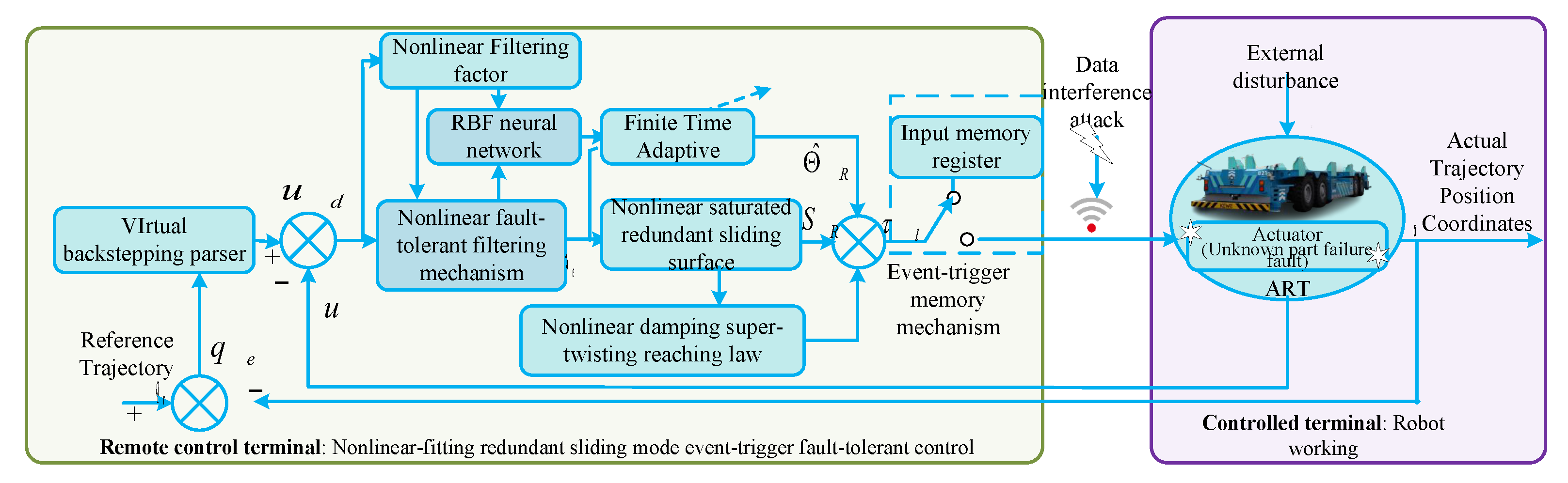
3. Controller Design
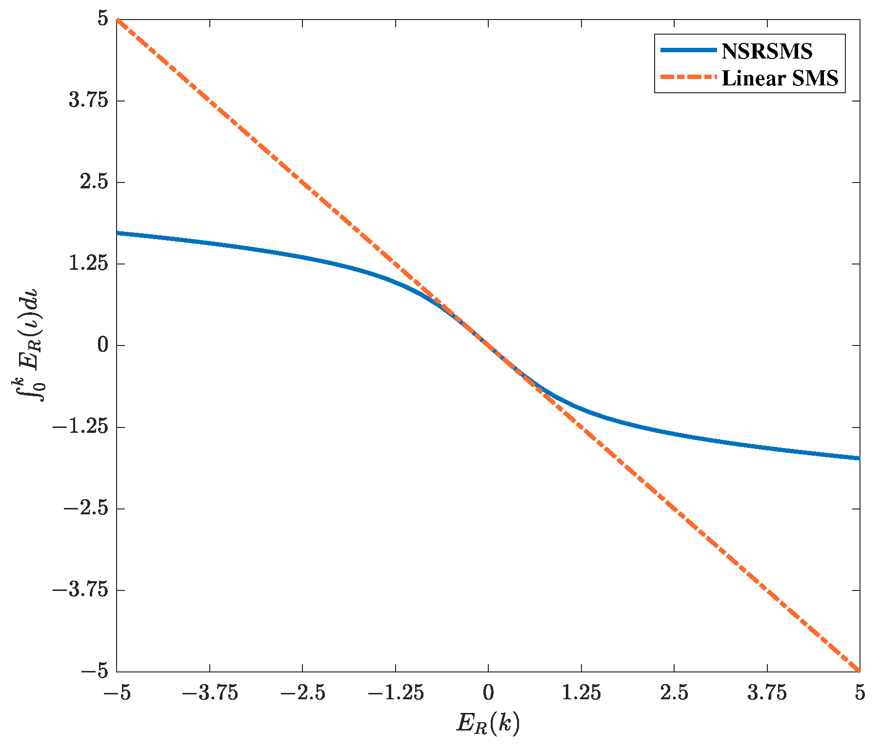
3.1. Nonlinear Saturation Fault-Tolerant Filtering Mechanism
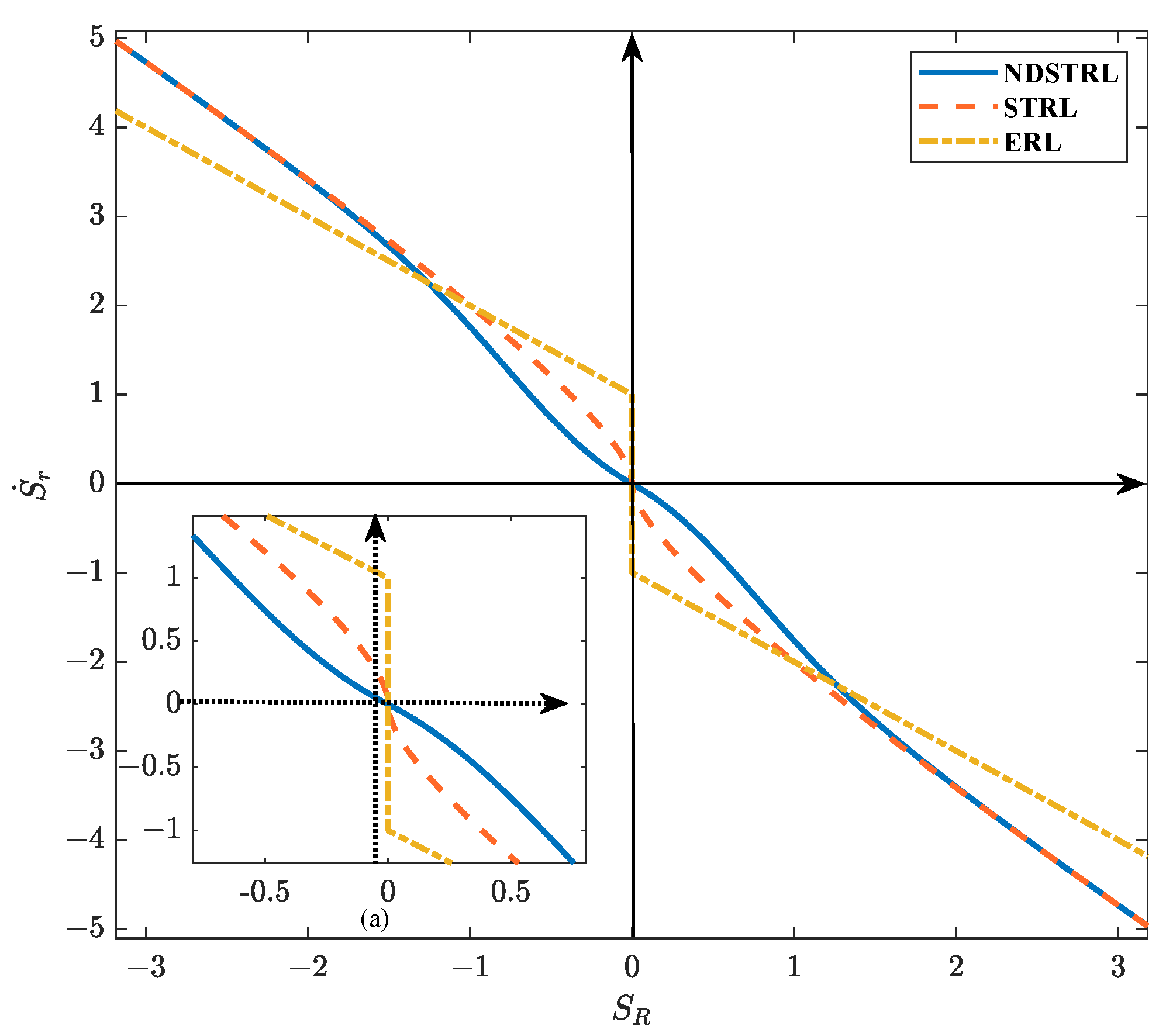
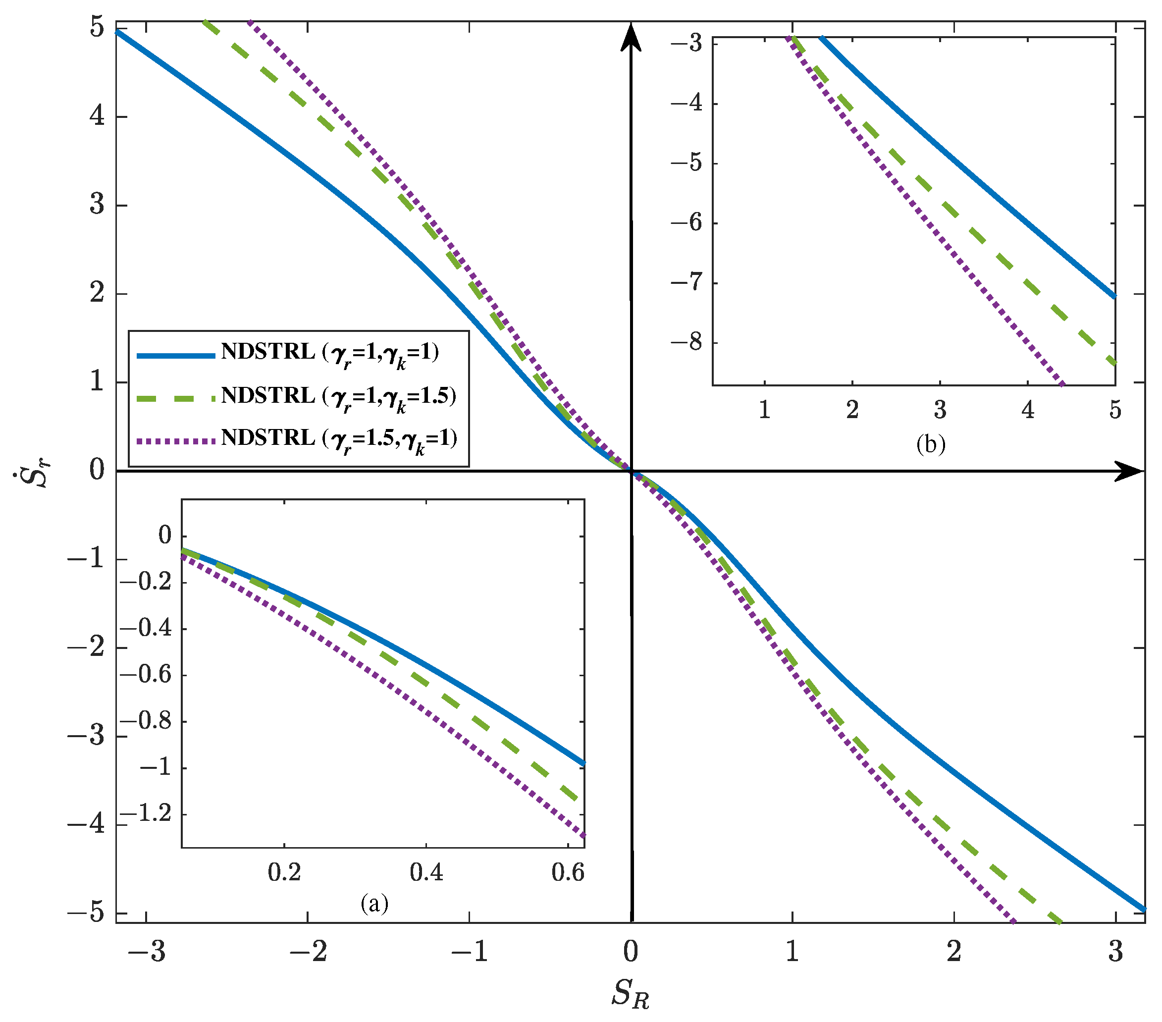
3.2. Design of Nonlinear-Fitting, Redundant, Sliding Mode, Event-Trigger Fault-Tolerant Control
3.3. Theoretical Proof
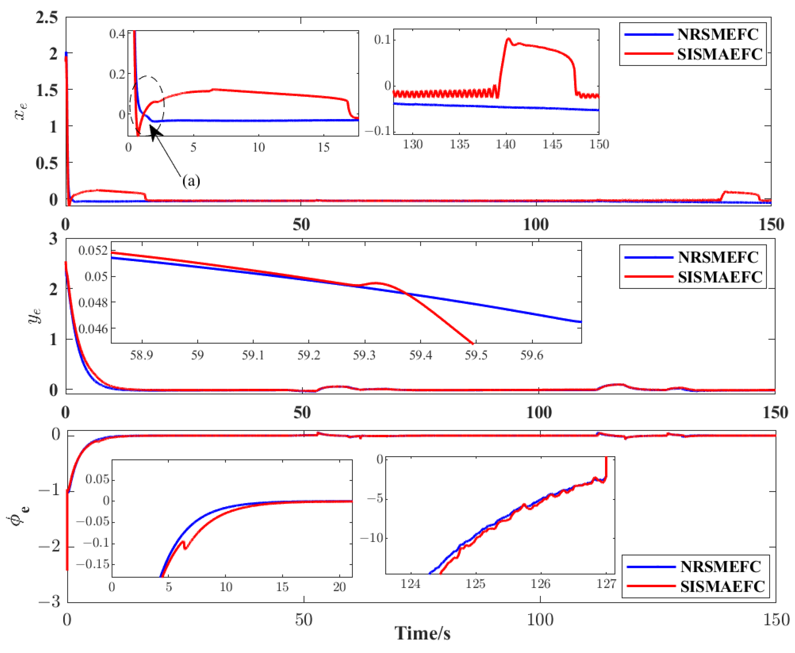
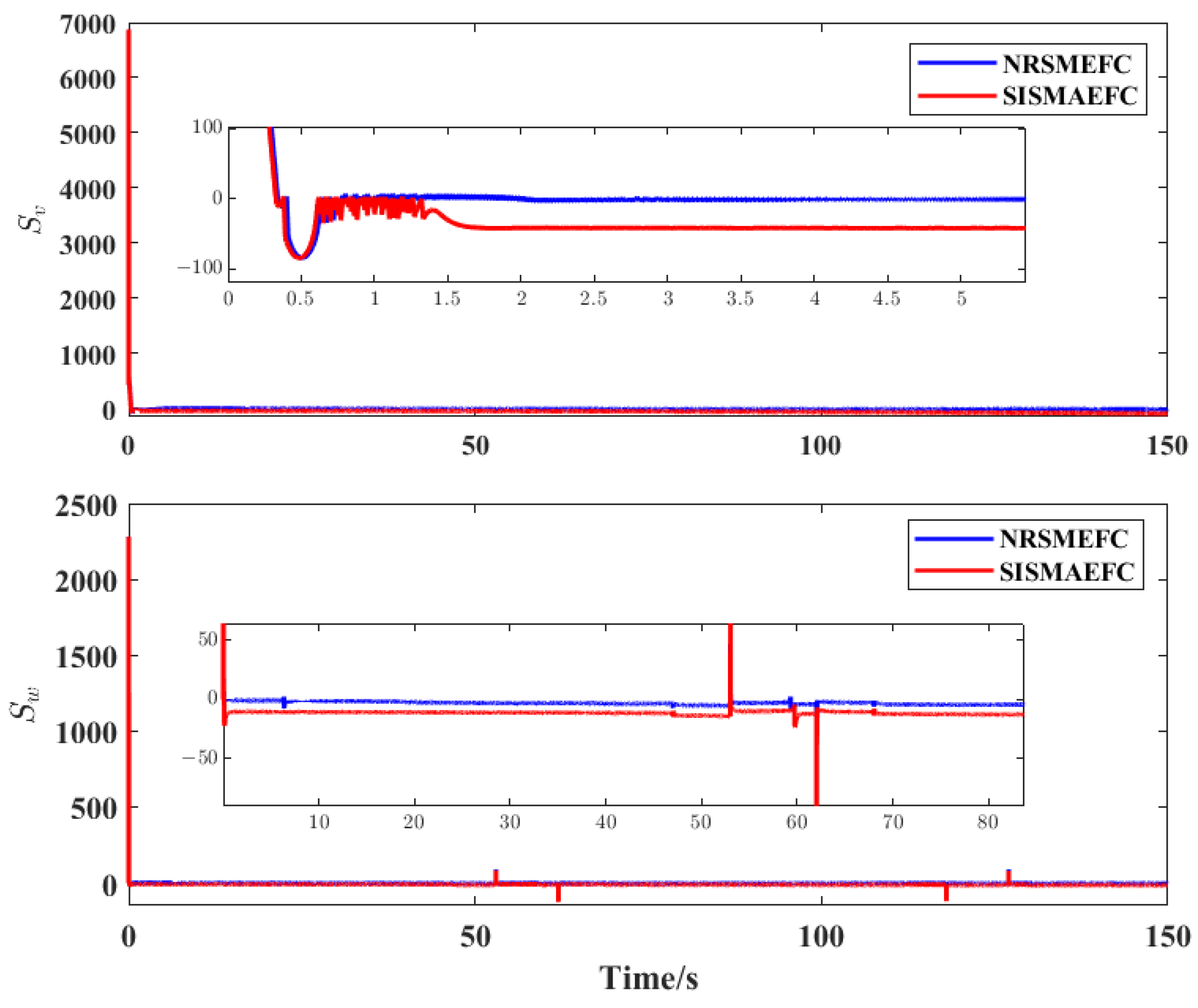
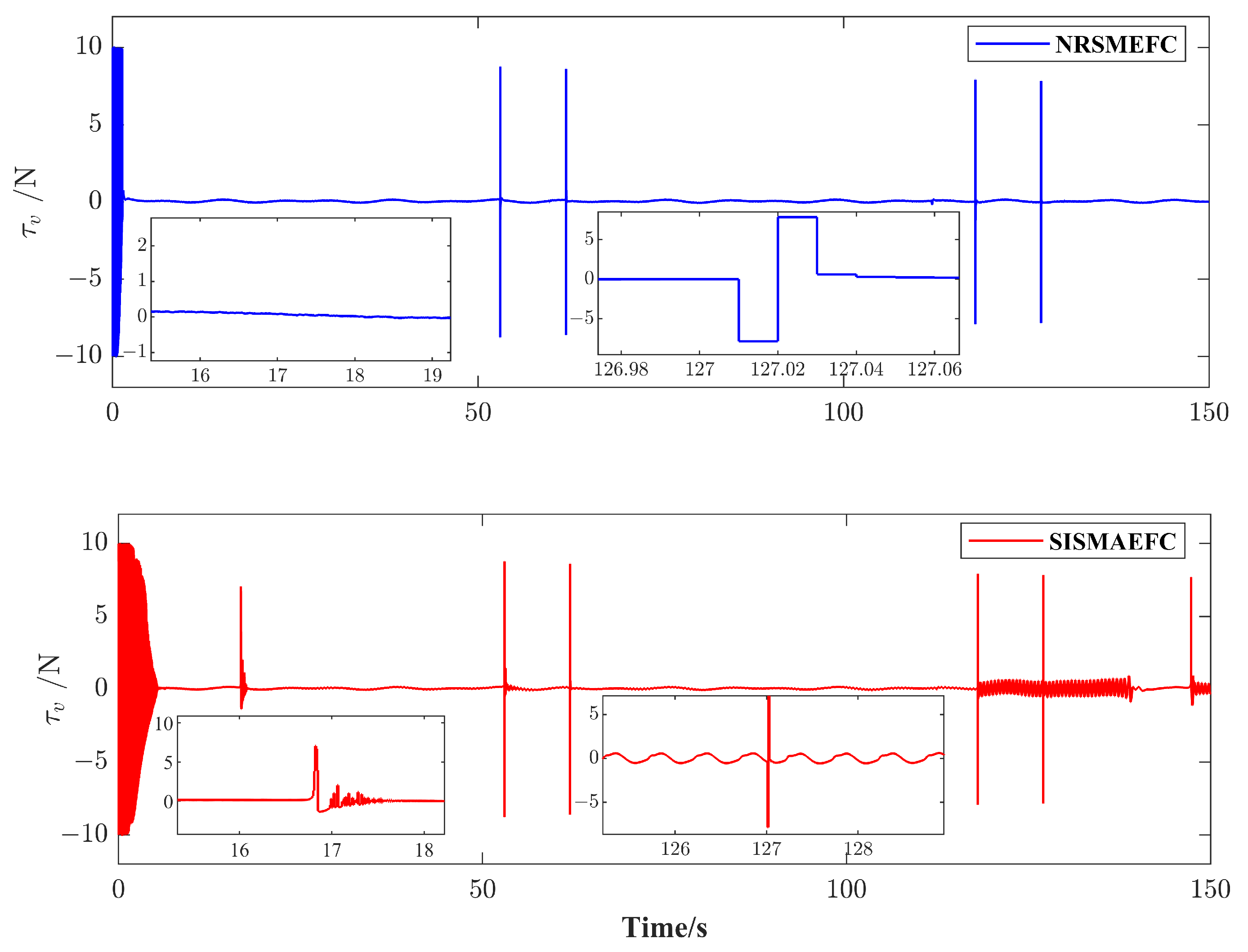
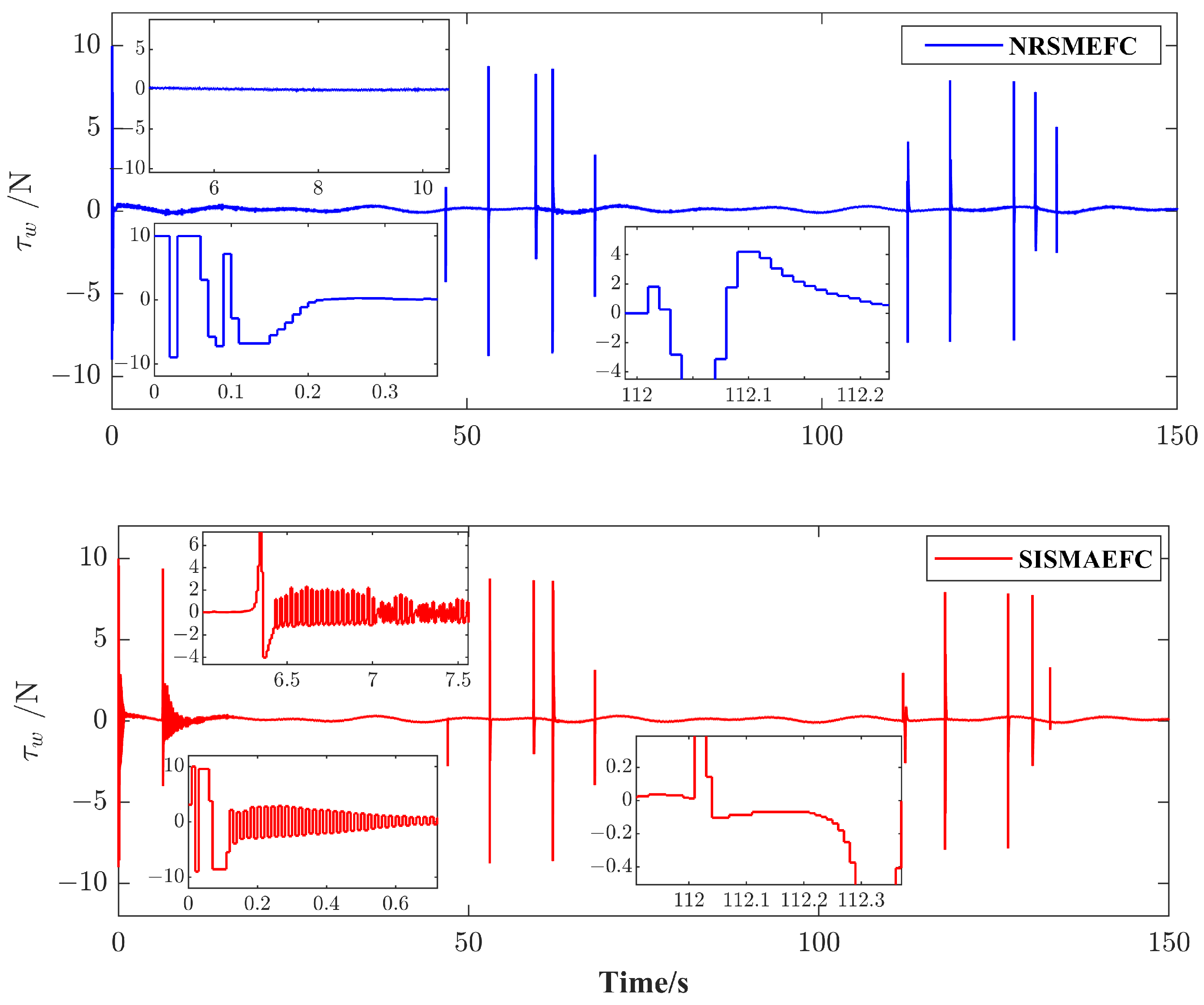
4. Simulation Results and Analysis
5. Conclusions
Author Contributions
Funding
Institutional Review Board Statement
Informed Consent Statement
Data Availability Statement
Conflicts of Interest
Abbreviations
| NSRSMS | New type of nonlinear, saturated, redundant sliding surface |
| NDSTRL | Nonlinear-damping, super-twisting reaching law |
| MIAC | Mean integration absolute control |
| MISE | Mean integration square error |
References
- Yoerger, D.R.; Jakuba, M.; Bradley, A.M.; Bingham, B. Techniques for Deep Sea Near Bottom Survey Using an Autonomous Underwater Vehicle. Int. J. Robot. Res. 2007, 26, 41–54. [Google Scholar] [CrossRef]
- Yang, J.; Sun, R.; Cui, J.; Ding, X. Application of composite fuzzy-PID algorithm to suspension system of Maglev train. In Proceedings of the 30th Annual Conference of IEEE Industrial Electronics Society, Busan, Republic of Korea, 2–6 November 2004. [Google Scholar]
- Jiang, G.P.; Wei, X.Z. An LMI criterion for linear-state-feedback based chaos synchronization of a class of chaotic systems. Chaos Solitons Fractals 2005, 26, 142–149. [Google Scholar] [CrossRef]
- Zhao, X.; Yang, H.; Xia, W.; Wang, X. Adaptive Fuzzy Hierarchical Sliding-Mode Control for a Class of MIMO Nonlinear Time-Delay Systems With Input Saturation. J. IEEE Trans. Fuzzy Syst. 2016, 25, 1061–1077. [Google Scholar] [CrossRef]
- Levant, A. Quasi-Continuous High-Order Sliding-Mode Controllers. In Proceedings of the 42nd IEEE Conference on Decision and Control Maui, Maui, HI, USA, 9–12 December 2003. [Google Scholar]
- Bartoszewicz, A. A new reaching law for sliding mode control of continuous time systems with constraints. J. Trans. Inst. Meas. Control 2014, 37, 515–521. [Google Scholar] [CrossRef]
- Ma, H.; Wu, J.; Xiong, Z.A. Novel Exponential Reaching Law of Discrete-Time Sliding-Mode Control. J. IEEE Trans. Ind. Electron. 2017, 64, 3840–3850. [Google Scholar] [CrossRef]
- Fallaha, C.J.; Saad, M.; Kanaan, H.Y.; Al-Haddad, K. Sliding-Mode Robot Control With Exponential Reaching Law. J. IEEE Trans. Ind. Electron. 2011, 58, 600–610. [Google Scholar] [CrossRef]
- Bartoszewicz, A. Pawe Latosiński. Discrete time sliding mode control with reduced switching—A new reaching law approach. J. Int. J. Robust Nonlinear Control 2016, 26, 47–68. [Google Scholar] [CrossRef]
- Chakrabarty, S.; Bandyopadhyay, B. A generalized reaching law with different convergence rates. J. Autom. Oxf. 2016, 63, 34–37. [Google Scholar] [CrossRef]
- Baek, J.; Jin, M.; Han, S. A New Adaptive Sliding Mode Control Scheme for Application to Robot Manipulators. J. IEEE Trans. Ind. Electron. 2016, 63, 3628–3637. [Google Scholar] [CrossRef]
- Niu, Y.; Lam, J.; Wang, X.; Ho, D.W. Neural adaptive sliding mode control for a class of nonlinear neutral delay systems. J. Dyn. Syst. Meas. Control 2008, 130, 758–767. [Google Scholar] [CrossRef]
- Kang, Z.; Limei, W.; Xin, F. High-order fast nonsingular terminal sliding mode control of permanent magnet linear motor based on double disturbance observer. IEEE Trans. Ind. Appl. 2022, 58, 3696–3705. [Google Scholar]
- Wang, Y.; Peng, J.; Zhu, K.; Chen, B.; Wu, H. Adaptive PID-fractional-order nonsingular terminal sliding mode control for cable-driven manipulators using time-delay estimation. Int. J. Syst. Sci. 2020, 51, 3118–3133. [Google Scholar] [CrossRef]
- Shao, K.; Zheng, J.; Huang, K.; Wang, H.; Man, Z.; Fu, M. Finite-Time Control of a Linear Motor Positioner Using Adaptive Recursive Terminal Sliding Mode. IEEE Trans. Ind. Electron. 2020, 67, 6659–6668. [Google Scholar] [CrossRef]
- Wang, Y.; Zhu, B.; Zhang, H.; Zheng, W.X. Functional observer-based finite-time adaptive ISMC for continuous systems with unknown nonlinear function. J. Autom. 2021, 125, 109468. [Google Scholar] [CrossRef]
- Sui, S.; Tong, S.; Chen, C. Finite-Time Filter Decentralized Control for Nonstrict-Feedback Nonlinear Large-Scale Systems. J. IEEE Trans. Fuzzy Syst. 2018, 26, 3289–3300. [Google Scholar] [CrossRef]
- Chen, M.; Wang, H.; Liu, X.; Hayat, T.; Alsaadi, F.E. Adaptive finite-time dynamic surface tracking control of nonaffine nonlinear systems with dead zone. J. Neurocomputing 2019, 366, 66–73. [Google Scholar] [CrossRef]
- Wang, H.; Liu, P.X.; Zhao, X.; Liu, X. Adaptive Fuzzy Finite-Time Control of Nonlinear Systems with Actuator Faults. J. IEEE Trans. Cybern. 2019, 99, 1–12. [Google Scholar]
- Wang, F.; Zhang, X. Adaptive Finite Time Control of Nonlinear Systems Under Time-Varying Actuator Failures. J. IEEE Trans. Syst. Man, Cybern. 2019, 49, 1845–1852. [Google Scholar] [CrossRef]
- Fang, W.A.; Gl, B. Fixed-time control design for nonlinear uncertain systems via adaptive method. J. Syst. Control Lett. 2020, 140, 104704. [Google Scholar]
- Ba, D.; Li, Y.X.; Tong, S. Fixed-time adaptive neural tracking control for a class of uncertain nonstrict nonlinear systems. J. Neurocomputing 2019, 363, 273–280. [Google Scholar] [CrossRef]
- Zuo, Z. Non-singular fixed-time terminal sliding mode control of non-linear systems. J. IET Control Theory Appl. 2014, 9, 545–552. [Google Scholar] [CrossRef]
- Liu, W.; Jian, T.; Yang, H.; Li, S.; Wang, H.; Wang, Y. Tunable Multichannel Adaptive Detector for Mismatched Subspace Signals. J. Electron. Inf. Technol. 2016, 38, 3011–3017. [Google Scholar]
- Liu, W.; Liu, J.; Huang, L.; Yang, Z.; Yang, H.; Wang, Y.L. Distributed Target Detectors With Capabilities of Mismatched Subspace Signal Rejection. J. Abbr. 2017, 53, 888–900. [Google Scholar] [CrossRef]
- Yang, F.; Zhang, H.; Jiang, B.; Liu, X. Adaptive reconfigurable control of systems with time-varying delay against unknown actuator faults. J. Int. J. Adapt. Control Signal Process. 2013, 28, 1206–1226. [Google Scholar] [CrossRef]
- Li, L.; Luo, H.; Ding, S.X.; Yang, Y.; Peng, K. Performance-based fault detection and fault-tolerant control for automatic control systems. J. Autom. 2019, 99, 308–316. [Google Scholar] [CrossRef]
- Zuo, Z.; Ho, D.; Wang, Y. Fault tolerant control for singular systems with actuator saturation and nonlinear perturbation. J. Autom. 2010, 46, 569–576. [Google Scholar] [CrossRef]
- Zhang, G.; Gao, S.; Li, J.; Zhang, W. Adaptive neural fault-tolerant control for course tracking of unmanned surface vehicle with event-triggered input. J. Proc. Inst. Mech. Eng. Part I J. Syst. Control Eng. 2021, 235, 1594–1604. [Google Scholar] [CrossRef]
- Zhang, X.M.; Han, Q.L. Event-triggered dynamic output feedback control for networked control systems. J. IET Control Theory Appl. 2014, 8, 226–234. [Google Scholar] [CrossRef]
- Domingo, M.C. Securing underwater wireless communication networks. J. IEEE Wirel. Commun. 2011, 18, 22–28. [Google Scholar] [CrossRef]
- Chen, Q.; Zhang, Q.; Hu, Y.; Liu, Y.; Wu, H. Euclidean distance damping–based adaptive sliding mode fault-tolerant event-triggered trajectory-tracking control. Proc. Inst. Mech. Eng. Part I J. Syst. Control. Eng. 2022. [Google Scholar] [CrossRef]
- Zhang, C.; Su, J.; Zhang, W.; Zhou, J. Design of Crawler Mobile Car with Infrared Remote Control. In Proceedings of the 2020 6th International Conference on Control, Automation and Robotics, Singapore, 20–23 April 2020. [Google Scholar]
- Najafi, B.; Ardabili, S.F. Application of ANFIS, ANN, and logistic methods in estimating biogas production from spent mushroom compost (SMC). Resour. Conserv. Recycl. 2018, 133, 169–178. [Google Scholar] [CrossRef]
- Sun, M.; Luan, T.; Liang, L. RBF neural network compensation-based adaptive control for lift-feedback system of ship fin stabilizers to improve anti-rolling effect. Ocean Eng. 2018, 163, 307–321. [Google Scholar] [CrossRef]
- Vinod, J.; Sarkar, B.K. Francis turbine electrohydraulic inlet guide vane control by artificial neural network 2 degree-of-freedom PID controller with actuator fault. Proc. Inst. Mech. Eng. 2021, 235, 1494–1509. [Google Scholar]
- Zhu, G.; Ma, Y.; Li, Z.; Malekian, R.; Sotelo, M. Adaptive neural output feedback control for MSVs with predefined performance. IEEE Trans. Veh. Technol. 2021, 70, 2994–3006. [Google Scholar] [CrossRef]
- Mobayen, S. Adaptive global sliding mode control of underactuated systems using a super-twisting scheme: An experimental study. J. Vib. Control. 2019, 25, 2215–2224. [Google Scholar] [CrossRef]
- Chen, Q.; Hu, Y.; Zhang, Q.; Jiang, J.; Chi, M.; Zhu, Y. Dynamic Damping-Based Terminal Sliding Mode Event-Triggered Fault-Tolerant Pre-Compensation Stochastic Control for Tracked ROV. J. Mar. Sci. Eng. 2022, 10, 1228. [Google Scholar] [CrossRef]
- Chen, K.; Yao, L.; Zhang, D.; Wang, X.; Chang, X.; Nie, F. A Semisupervised Recurrent Convolutional Attention Model for Human Activity Recognition. IEEE Trans. Neural Networks Learn. Syst. 2020, 31, 1747–1756. [Google Scholar] [CrossRef]
- Luo, M.; Chang, X.; Nie, L.; Yang, Y.; Hauptmann, A.G.; Zheng, Q. An Adaptive Semisupervised Feature Analysis for Video Semantic Recognition. IEEE Trans. Cybern. 2018, 48, 648–660. [Google Scholar] [CrossRef]
- Zhang, D.; Yao, L.; Chen, K.; Wang, S.; Chang, X.; Liu, Y. Making Sense of Spatio-Temporal Preserving Representations for EEG-Based Human Intention Recognition. IEEE Trans. Cybern. 2020, 50, 3033–3044. [Google Scholar] [CrossRef]


| Evaluation Criteria | MIAC | MISE |
|---|---|---|
| Algorithm in this paper | [0.90, 2.03] | [8.307, 8.844, 3.16] |
| Comparison algorithm | [1.107, 3.75] | [10.74, 10.13, 3.57] |
Disclaimer/Publisher’s Note: The statements, opinions and data contained in all publications are solely those of the individual author(s) and contributor(s) and not of MDPI and/or the editor(s). MDPI and/or the editor(s) disclaim responsibility for any injury to people or property resulting from any ideas, methods, instructions or products referred to in the content. |
© 2023 by the authors. Licensee MDPI, Basel, Switzerland. This article is an open access article distributed under the terms and conditions of the Creative Commons Attribution (CC BY) license (https://creativecommons.org/licenses/by/4.0/).
Share and Cite
Zhu, Y.; Zhang, Q.; Liu, Y.; Hu, Y.; Zhang, S. Neural Network, Nonlinear-Fitting, Sliding Mode, Event-Triggered Control under Abnormal Input for Port Artificial Intelligence Transportation Robots. J. Mar. Sci. Eng. 2023, 11, 659. https://doi.org/10.3390/jmse11030659
Zhu Y, Zhang Q, Liu Y, Hu Y, Zhang S. Neural Network, Nonlinear-Fitting, Sliding Mode, Event-Triggered Control under Abnormal Input for Port Artificial Intelligence Transportation Robots. Journal of Marine Science and Engineering. 2023; 11(3):659. https://doi.org/10.3390/jmse11030659
Chicago/Turabian StyleZhu, Yaping, Qiang Zhang, Yang Liu, Yancai Hu, and Sihang Zhang. 2023. "Neural Network, Nonlinear-Fitting, Sliding Mode, Event-Triggered Control under Abnormal Input for Port Artificial Intelligence Transportation Robots" Journal of Marine Science and Engineering 11, no. 3: 659. https://doi.org/10.3390/jmse11030659