
Uncertainty Assessment of Wave Elevation Field Measurement Using a Depth Camera

Abstract
:1. Introduction
2. Test Setup
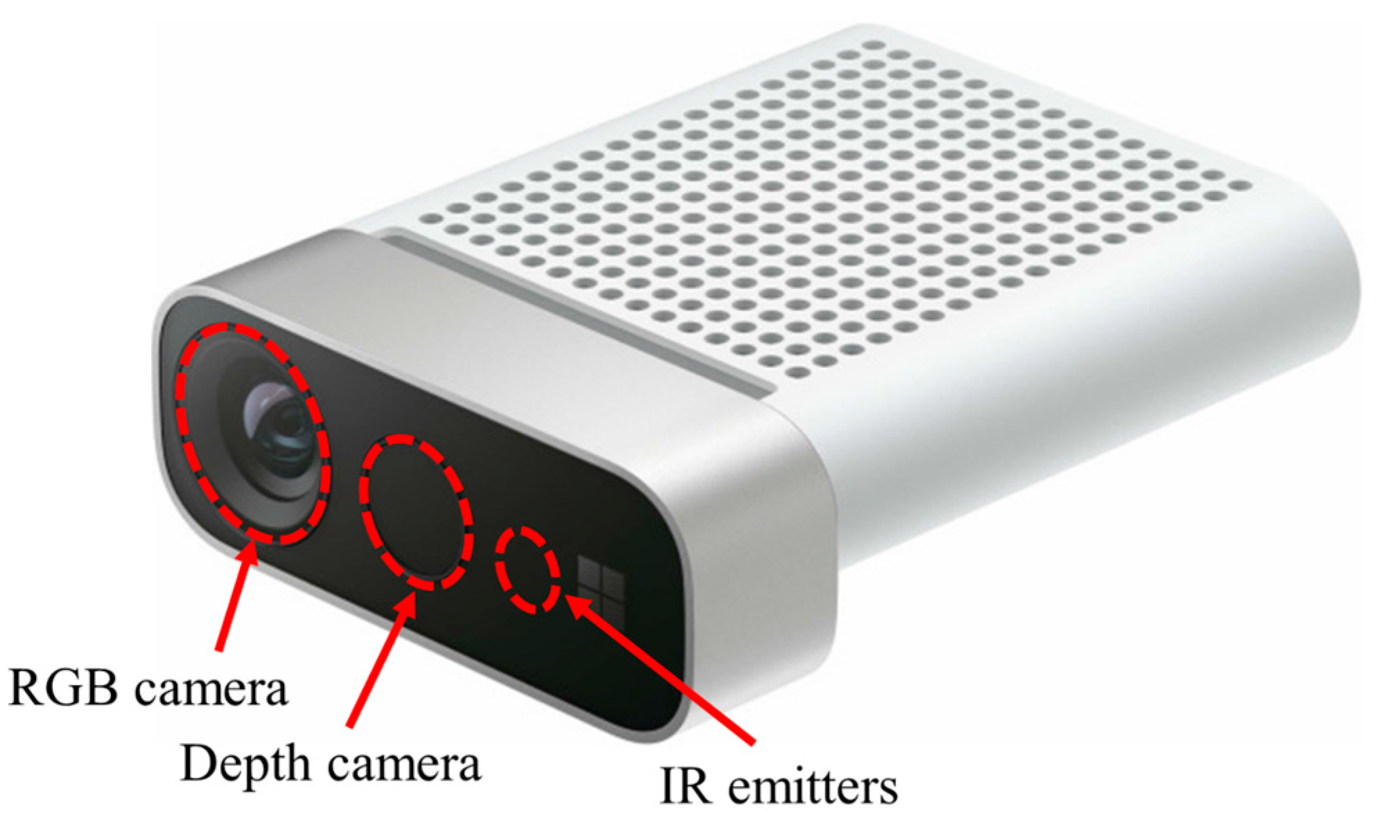
2.1. Depth Camera
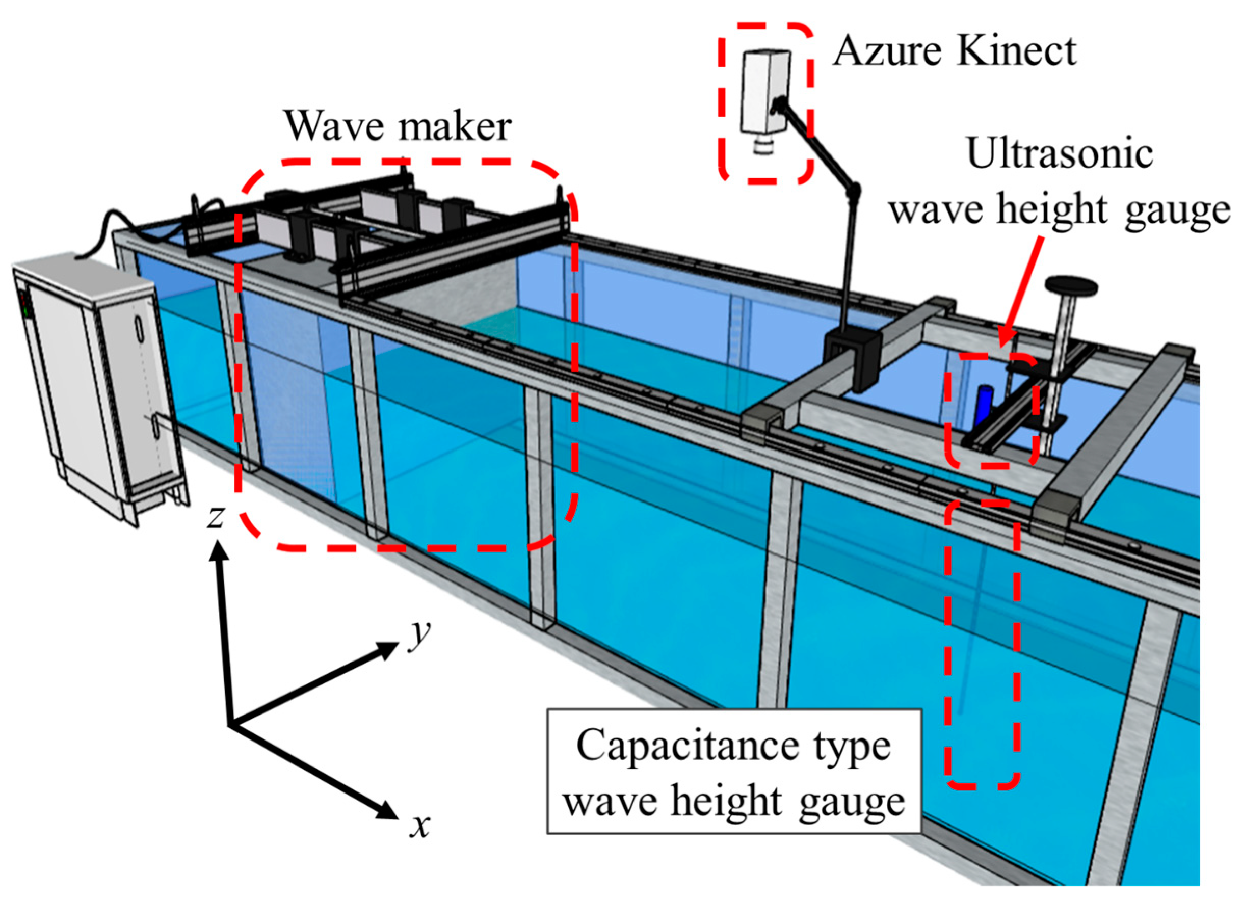
2.2. Wave Flume
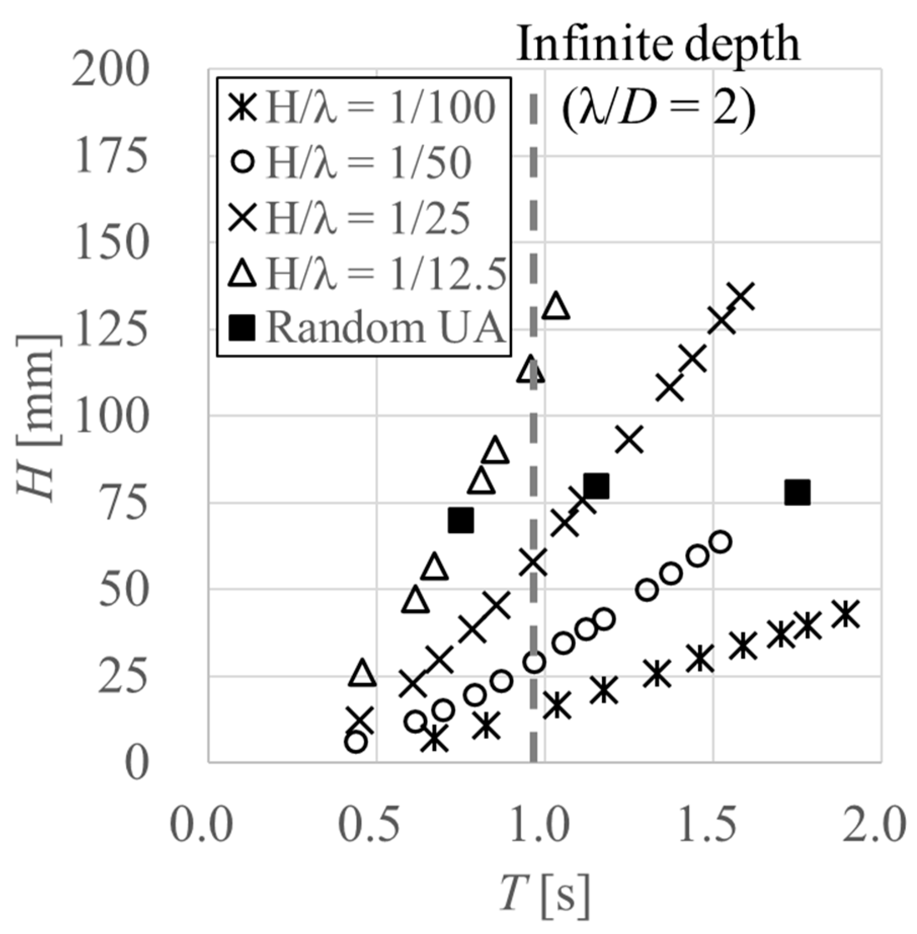
2.3. Test Cases
3. Principles of Test Uncertainty Assessment
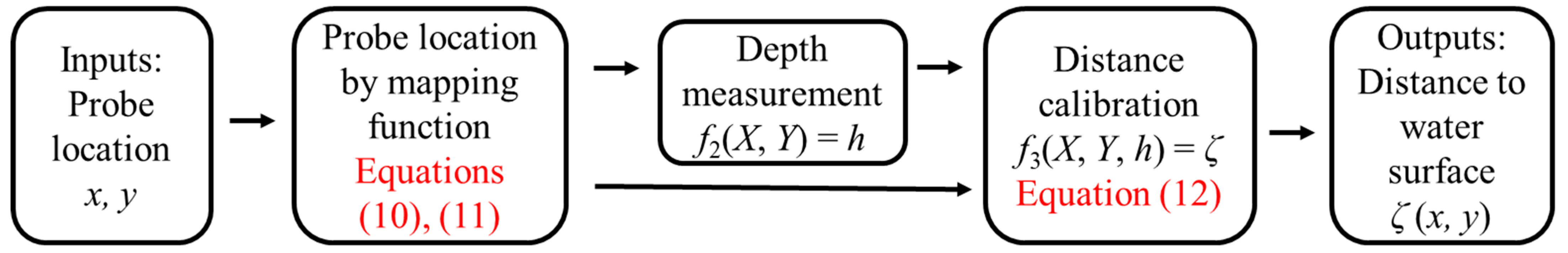
4. Calibration Procedure
5. Test Uncertainty Assessment
6. Conclusions
Author Contributions
Funding
Institutional Review Board Statement
Informed Consent Statement
Data Availability Statement
Conflicts of Interest
References
- Huang, W.; Xiao, H. Numerical modeling of dynamic wave force acting on Escambia Bay Bridge deck during Hurricane Ivan. J. Waterw. Port Coast. Ocean Eng. 2009, 135, 164–175. [Google Scholar] [CrossRef]
- Guo, A.; Fang, Q.; Bai, X.; Li, H. Hydrodynamic experiment of the wave force acting on the superstructures of coastal bridges. J. Bridge Eng. 2015, 20, 04015012. [Google Scholar] [CrossRef]
- Azadbakht, M.; Yim, S.C. Simulation and estimation of tsunami loads on bridge superstructures. J. Watew. Port Coast. Ocean Eng. 2015, 141, 04014031. [Google Scholar] [CrossRef]
- Yan, J.; Korobenko, A.; Deng, X.; Bazilevs, Y. Computational free-surface fluid-structure interaction with application to floating offshore wind turbines. Comput. Fluids 2016, 141, 155–174. [Google Scholar] [CrossRef]
- Pham, T.D.; Shin, H. The effect of the second-order wave lads on drift motion of a semi-submersible floating offshore wind turbine. J. Mar. Sci. Eng. 2020, 8, 859. [Google Scholar] [CrossRef]
- Thiagarajan, K.; Moreno, J. Wave induced effects on the hydrodynamic coefficients of an oscillating heave plate in offshore wind turbines. J. Mar. Sci. Eng. 2020, 8, 622. [Google Scholar] [CrossRef]
- Zhao, Y.; Guan, C.; Bi, C.; Liu, H.; Cui, Y. Experimental investigations on hydrodynamic responses of a semi-submersible offshore fish farm in waves. J. Mar. Sci. Eng. 2019, 7, 238. [Google Scholar] [CrossRef] [Green Version]
- Gatin, I.; Vukcevic, V.; Jasak, H.; Seo, J.; Rhee, S.H. CFD verification and validation of green sea loads. Ocean Eng. 2018, 148, 500–515. [Google Scholar] [CrossRef]
- Azman, N.U.; Husain, M.K.A.; Zaki, N.I.M.; Soom, E.M.; Mukhlas, N.A.; Ahmad, S.Z.A.S. Structural integrity of fixed offshore platforms by incorporating wave-in-deck. J. Mar. Sci. Eng. 2021, 9, 1027. [Google Scholar] [CrossRef]
- Jiang, C.; el Moctar, O.; Schellin, T.E. Hydrodynamic sensitivity of moored and articulated multibody offshore structures in waves. J. Mar. Sci. Eng. 2021, 9, 1028. [Google Scholar] [CrossRef]
- Begovic, E.; Bertorello, C.; Pennino, S. Experimental seakeeping assessment of a warped planing hull model series. Ocean Eng. 2014, 83, 1–15. [Google Scholar] [CrossRef]
- Park, D.-M.; Lee, J.; Kim, Y. Uncertainty analysis for added resistance experiment of KVLCC2 ship. Ocean Eng. 2015, 95, 143–156. [Google Scholar] [CrossRef]
- Seo, J.; Choi, H.; Jeong, U.-C.; Lee, D.K.; Rhee, S.H.; Jung, C.-M.; Yoo, J. Model tests on resistance and seakeeping performance of wave-piercing high-speed vessel with spray rails. Int. J. Nav. Archit. Ocean Eng. 2016, 8, 442–455. [Google Scholar] [CrossRef] [Green Version]
- Begovic, E.; Bertorello, C.; Pennino, S.; Piscopo, V.; Scamardella, A. Statistical analysis of planing hull motions and accelerations in irregular head sea. Ocean Eng. 2016, 112, 253–264. [Google Scholar] [CrossRef]
- Kim, W.J.; Van, S.H.; Kim, D.H. Measurement of flows around modern commercial ship models. Exp. Fluids 2001, 31, 567–578. [Google Scholar] [CrossRef]
- Longo, J.; Stern, F. Uncertainty assessment for towing tank tests with example for surface combatant DTMB Model 5415. J. Ship Res. 2005, 49, 55–68. [Google Scholar] [CrossRef]
- Kashiwagi, M. Hydrodynamic study on added resistance using unsteady wave analysis. J. Ship Res. 2013, 57, 220–240. [Google Scholar]
- Lee, D.; Hong, S.Y.; Lee, G.-J. Theoretical and experimental study on dynamic behavior of a damaged ship in waves. Ocean Eng. 2007, 34, 21–31. [Google Scholar] [CrossRef]
- Lee, S.; You, J.-M.; Lee, H.-H.; Lim, T.; Park, S.T.; Seo, J.; Rhee, S.H.; Rhee, K.-P. Experimental study on the six degree-of-freedom motions of a damaged ship floating in regular waves. IEEE J. Ocean. Eng. 2016, 41, 40–49. [Google Scholar]
- Espinoza Haro, M.P.; Seo, J.; Sadat-Hosseini, H.; Seok, W.-C.; Rhee, S.H.; Stern, F. Numerical simulations for the safe return to port of a damaged passenger ship in head or following seas. Ocean Eng. 2017, 143, 305–318. [Google Scholar] [CrossRef]
- Begovic, E.; Bertorello, C.; Bove, A.; Garme, K.; Lei, X.; Persson, J.; Petrone, G.; Razola, M.; Rosen, A. Experimental modelling of local structure responses for high-speed planing craft in waves. Ocean Eng. 2020, 216, 107986. [Google Scholar] [CrossRef]
- Tavakoli, S.; Bilandi, R.N.; Mancini, S.; De Luca, F.; Dashtimanesh, A. Dynamic of a planing hull in regular waves: Comparison of experimental, numerical and mathematical methods. Ocean Eng. 2020, 217, 107959. [Google Scholar] [CrossRef]
- Metcalf, B.; Longo, J.; Ghosh, S.; Stern, F. Unsteady free-surface wave-induced boundary-layer separation for a surface-piercing NACA 0024 foil: Towing tank experiments. J. Fluids Struct. 2006, 22, 77–98. [Google Scholar] [CrossRef]
- Liu, J.; Guo, A.; Li, H. Experimental investigation on three-dimensnional structures of wind wave surfaces. Ocean Eng. 2022, 265, 112628. [Google Scholar] [CrossRef]
- Lev, S. Laboratory study of temporal and spatial evolution of waves excited on water surface initially at rest by impulsive wind forcing. Procedia IUTAM 2018, 26, 153–161. [Google Scholar]
- Benetazzo, A.; Fedele, F.; Gallego, G.; Shih, P.C.; Yezzi, A. Offshore stereo measurements of gravity waves. Coast. Eng. 2012, 64, 127–138. [Google Scholar] [CrossRef] [Green Version]
- Benetazzo, A.; Barbariol, F.; Bergamasco, F.; Torsello, A.; Carniel, S.; Sclavo, M. Observation of extreme sea waves in a space-time ensemble. J. Phys. Oceanogr. 2015, 45, 2261–2275. [Google Scholar] [CrossRef] [Green Version]
- Benetazzo, A.; Barbariol, F.; Bergamasco, F.; Torsello, A.; Carniel, S.; Sclavo, M. Stereo wave imaging from moving vessels: Practical use and applications. Coast. Eng. 2016, 109, 114–127. [Google Scholar] [CrossRef]
- van Meerkerk, M.; Poelma, C.; Westerweel, J. Scanning stereo-PLIF method for free surface measurements in large 3D domains. Exp. Fluids 2020, 61, 19. [Google Scholar] [CrossRef] [Green Version]
- Gomit, G.; Chatellier, L.; David, L. Free-surface flow measurements by non-intrusive methods: A survey. Exp. Fluids 2022, 63, 94. [Google Scholar] [CrossRef]
- Zarruk, G.A. Measurement of free surface deformation in PIV images. Meas. Sci. Technol. 2005, 16, 1970–1975. [Google Scholar] [CrossRef]
- Chatellier, L.; Jarny, S.; Gibouin, F.; David, L. A parametric PIV/DIC method for the measurement of free surface flows. Exp. Fluids 2013, 54, 1488. [Google Scholar] [CrossRef]
- Caplier, C.; Rousseaux, G.; Calluaud, D.; David, L. Energy distribution in shallow water ship wakes from a spectral analysis of the wave field. Phys. Fluids 2016, 28, 107104. [Google Scholar] [CrossRef]
- Tsubaki, R.; Fujita, I. Stereoscopic measurement of a fluctuating free surface with discontinuities. Meas. Sci. Technol. 2005, 16, 1894–1902. [Google Scholar] [CrossRef]
- Evers, F.M. Videometric water surface tracking of spatial impulse wave propagation. J. Vis. 2018, 21, 903–907. [Google Scholar] [CrossRef] [Green Version]
- Gomit, G.; Chatellier, L.; Calluaud, D.; David, L.; Frechou, D.; Boucheron, R.; Perelman, O.; Hubert, C. Large-scale free surface measurement for the analysis of ship waves in a towing tank. Exp. Fluids 2015, 56, 184. [Google Scholar] [CrossRef]
- Sanada, Y.; Toda, Y.; Hamachi, S. Free surface measurement by reflected light image. In Proceedings of the 25th International Towing Tank Conference, Fukuoka, Japan, 14–20 September 2008. [Google Scholar]
- Jähne, B.; Schmidt, M.; Rocholz, R. Combined optical slope/height measurements of short wind waves: Principle and calibration. Meas. Sci. Technol. 2005, 16, 1937–1944. [Google Scholar] [CrossRef]
- Zappa, C.J.; Banner, M.L.; Schultz, H.; Corrada-Emmanuel, A.; Wolff, L.B.; Yalcin, J. Retrieval of short ocean wave slope using polarimetric imaging. Meas. Sci. Technol. 2008, 19, 055503. [Google Scholar] [CrossRef]
- Park, H.S.; Sim, J.S.; Yoo, J.; Lee, D.Y. The breaking wave measurement using terrestrial LIDAR: Validation with field experiment on the Mallipo Beach. J. Coast. Res. 2011, 64, 1718–1721. [Google Scholar]
- Deems, J.S.; Painter, T.H.; Finnegan, D.C. Lidar measurement of snow depth: A review. J. Glaciol. 2013, 59, 467–479. [Google Scholar] [CrossRef] [Green Version]
- Toselli, F.; De Lillo, F.; Onorato, M.; Boffetta, G. Measuring surface gravity waves using a Kinect sensor. Eur. J. Mech. B Fluids 2019, 74, 260–264. [Google Scholar] [CrossRef] [Green Version]
- Kim, H.; Jeon, C.; Seo, J. Development of wave height field measurement system using a depth camera. J. Soc. Nav. Archit. Korea 2021, 58, 382–390. (In Korean) [Google Scholar] [CrossRef]
- Sciacchitano, A.; Wieneke, B. PIV uncertainty propagation. Meas. Sci. Technol. 2016, 27, 084006. [Google Scholar] [CrossRef] [Green Version]
- Han, B.W.; Seo, J.; Lee, S.J.; Seol, D.M.; Rhee, S.H. Uncertainty assessment for a towed underwater stereo PIV system by uniform flow measurement. Int. J. Nav. Archit. Ocean Eng. 2018, 10, 596–608. [Google Scholar] [CrossRef]
- Sciacchitano, A. Uncertainty quantification in particle image velocimetry. Meas. Sci. Technol. 2019, 30, 092001. [Google Scholar] [CrossRef] [Green Version]
- Bamji, C.S.; Mehta, S.; Thompson, B.; Elkhatib, T.; Wurster, S.; Akkaya, O.; Payne, A.; Godbaz, J.; Fenton, M.; Rajasekaran, V.; et al. IMpixel 65nm BSI 320MHz demodulated TOF Image sensor with 3μm global shutter pixels and analog binning. In Proceedings of the 2018 IEEE International Solid—State Circuits Conference—(ISSCC), San Francisco, CA, USA, 11–15 February 2018. [Google Scholar]
- Tölgyessy, M.; Dekan, M.; Chovanec, Ľ.; Hubinský, P. Evaluation of the Azure Kinect and its comparison to Kinect V1 and Kinect V2. Sensors 2021, 21, 413. [Google Scholar] [CrossRef] [PubMed]
- Microsoft Corporation. Microsoft Docs—Azure Kinect DK Documentation: Azure Kinect DK Hardware Specification; Microsoft Corporation: Redmond, WA, USA, 2021. [Google Scholar]
- Kim, H.; Oh, J.; Lew, J.; Rhee, S.H.; Kim, J.H. Wave and wave board motion of hybrid wave maker. J. Soc. Nav. Archit. Korea 2021, 58, 339–347. (In Korean) [Google Scholar] [CrossRef]
- ASME PTC 19.1-2005; Test Uncertainty. American Society of Mechanical Engineers (ASME): New York, NY, USA, 2005.
- Prasad, A.K. Stereoscopic particle image velocimetry. Exp. Fluids 2000, 29, 103–116. [Google Scholar] [CrossRef]
- Soloff, S.M.; Adrian, R.J.; Liu, Z.-C. Distortion compensation for generalized stereoscopic particle image velocimetry. Meas. Sci. Technol. 1997, 8, 1441–1454. [Google Scholar] [CrossRef]


| Mode | Resolution (Pixels) | Field of Interest (°) | Frame-Per-Second (Hz) | Operating Range (m) | Exposure Time (ms) |
|---|---|---|---|---|---|
| Narrow FoV—unbinned | 640 × 576 | 75 × 65 | 0, 5, 15, 30 | 0.5–3.86 | 12.8 |
| Narrow FoV—2 × 2 binned | 320 × 288 | 75 × 65 | 0, 5, 15, 30 | 0.5–5.46 | 12.8 |
| Wide FoV—2 × 2 binned | 512 × 512 | 120 × 120 | 0, 5, 15, 30 | 0.25–2.88 | 12.8 |
| Wide FoV—unbinned | 1024 × 1024 | 120 × 120 | 0, 5, 15 | 0.25–2.21 | 20.3 |
| Passive IR | 1024 × 1024 | Not applicable | 0, 5, 15, 30 | N/A | 1.6 |
| f1(X, Y) = x | f1(X, Y) = y | f3(X, Y, h) = ζ | |||
|---|---|---|---|---|---|
| α30 | 2.10 × 10⁻¹ | β30 | 4.48 × 10⁻² | γ1 | 0 |
| α21 | −1.87 × 10⁻³ | β21 | 1.61 × 10⁻⁵ | γ2 | −5.87 × 10⁻⁴ |
| α20 | 2.77 × 10⁻⁶ | β20 | 2.92 × 10⁻⁴ | γ3 | 9.1 × 10⁻¹ |
| α12 | 2.10 × 10⁻⁵ | β12 | 9.37 × 10⁻⁷ | ||
| α11 | −1.75 × 10⁻³ | β11 | −2.21 × 10⁻³ | ||
| α10 | 1.94 × 10⁻⁵ | β10 | −7.49 × 10⁻⁶ | ||
| α03 | −3.94 × 10⁻³ | β03 | 1.68 × 10⁻⁵ | ||
| α02 | −3.33 × 10⁻¹ | β02 | −3.71 × 10⁻³ | ||
| α01 | 2.94 | β01 | 3.01 | ||
| α00 | 0 | β00 | 0 | ||
| Wave Condition H/λ | Probe Location (f1) | Depth Measurement (f2) | Depth Calibration (f3) | Systematic Standard Uncertainty bζ (mm) | ||||
|---|---|---|---|---|---|---|---|---|
| θf1 | bX (mm) | bY (mm) | bf2 (mm) | θf3 | bf3 (mm) | |||
| Depth camera | 1/12.5 | 0.16 | 2.2 | 3.4 | 0.25 | 1.00 | 0.32 | 0.76 |
| 1/25 | 0.08 | 0.52 | ||||||
| 1/50 | 0.04 | 0.44 | ||||||
| Capacitance-type wave height gauge | 1/12.5 | 0.16 | 2 | 2 | - | 1.00 | 0.21 | 0.50 |
| 1/25 | 0.08 | 0.31 | ||||||
| 1/50 | 0.04 | 0.24 | ||||||
| Ultrasonic wave height gauge | 1/12.5 | 0.16 | 5 | 5 | - | 1.00 | 0.51 | 1.24 |
| 1/25 | 0.08 | 0.76 | ||||||
| 1/50 | 0.04 | 0.58 | ||||||
| H/λ | H (mm) | sζ1 (mm) | sζ2 (mm) | sζ (mm) | uζ (mm) | Uζ95 (mm) (Uζ95/H) | |
|---|---|---|---|---|---|---|---|
| Depth camera | 1/12.5 | 70 | 1.01 | 0.20 | 1.03 | 1.28 | 3.56 (5.1%) |
| 1/25 | 80 | 0.72 | 0.14 | 0.73 | 0.90 | 2.50 (3.1%) | |
| 1/50 | 78 | 0.805 | 0.16 | 0.82 | 0.93 | 2.58 (3.3%) | |
| Capacitance-type wave height gauge | 1/12.5 | 70 | 0.695 | 0.14 | 0.71 | 0.87 | 2.41 (3.4%) |
| 1/25 | 80 | 0.575 | 0.12 | 0.59 | 0.66 | 1.84 (2.3%) | |
| 1/50 | 78 | 0.465 | 0.09 | 0.47 | 0.53 | 1.47 (1.9%) | |
| Ultrasonic wave height gauge | 1/12.5 | 70 | - | ||||
| 1/25 | 80 | 0.87 | 0.17 | 0.89 | 1.17 | 3.25 (4.1%) | |
| 1/50 | 78 | 0.655 | 0.13 | 0.67 | 0.89 | 2.46 (3.2%) | |
Disclaimer/Publisher’s Note: The statements, opinions and data contained in all publications are solely those of the individual author(s) and contributor(s) and not of MDPI and/or the editor(s). MDPI and/or the editor(s) disclaim responsibility for any injury to people or property resulting from any ideas, methods, instructions or products referred to in the content. |
© 2023 by the authors. Licensee MDPI, Basel, Switzerland. This article is an open access article distributed under the terms and conditions of the Creative Commons Attribution (CC BY) license (https://creativecommons.org/licenses/by/4.0/).
Share and Cite
Kim, H.; Jeon, C.; Kim, K.; Seo, J. Uncertainty Assessment of Wave Elevation Field Measurement Using a Depth Camera. J. Mar. Sci. Eng. 2023, 11, 657. https://doi.org/10.3390/jmse11030657
Kim H, Jeon C, Kim K, Seo J. Uncertainty Assessment of Wave Elevation Field Measurement Using a Depth Camera. Journal of Marine Science and Engineering. 2023; 11(3):657. https://doi.org/10.3390/jmse11030657
Chicago/Turabian StyleKim, Hoyong, Chanil Jeon, Kiwon Kim, and Jeonghwa Seo. 2023. "Uncertainty Assessment of Wave Elevation Field Measurement Using a Depth Camera" Journal of Marine Science and Engineering 11, no. 3: 657. https://doi.org/10.3390/jmse11030657