
Study of the Optimal Grid Resolution and Effect of Wave–Wave Interaction during Simulation of Extreme Waves Induced by Three Ensuing Typhoons


Abstract
:1. Introduction
2. Three Successive Typhoons That Impacted Taiwan in September 2016
3. Data and Model
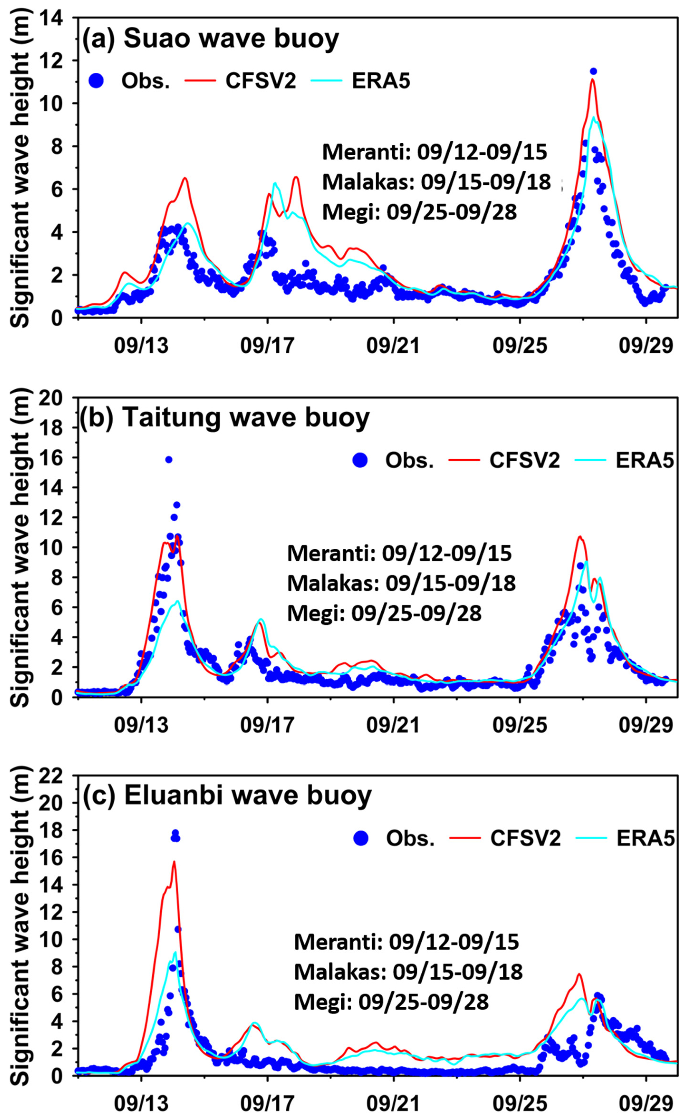
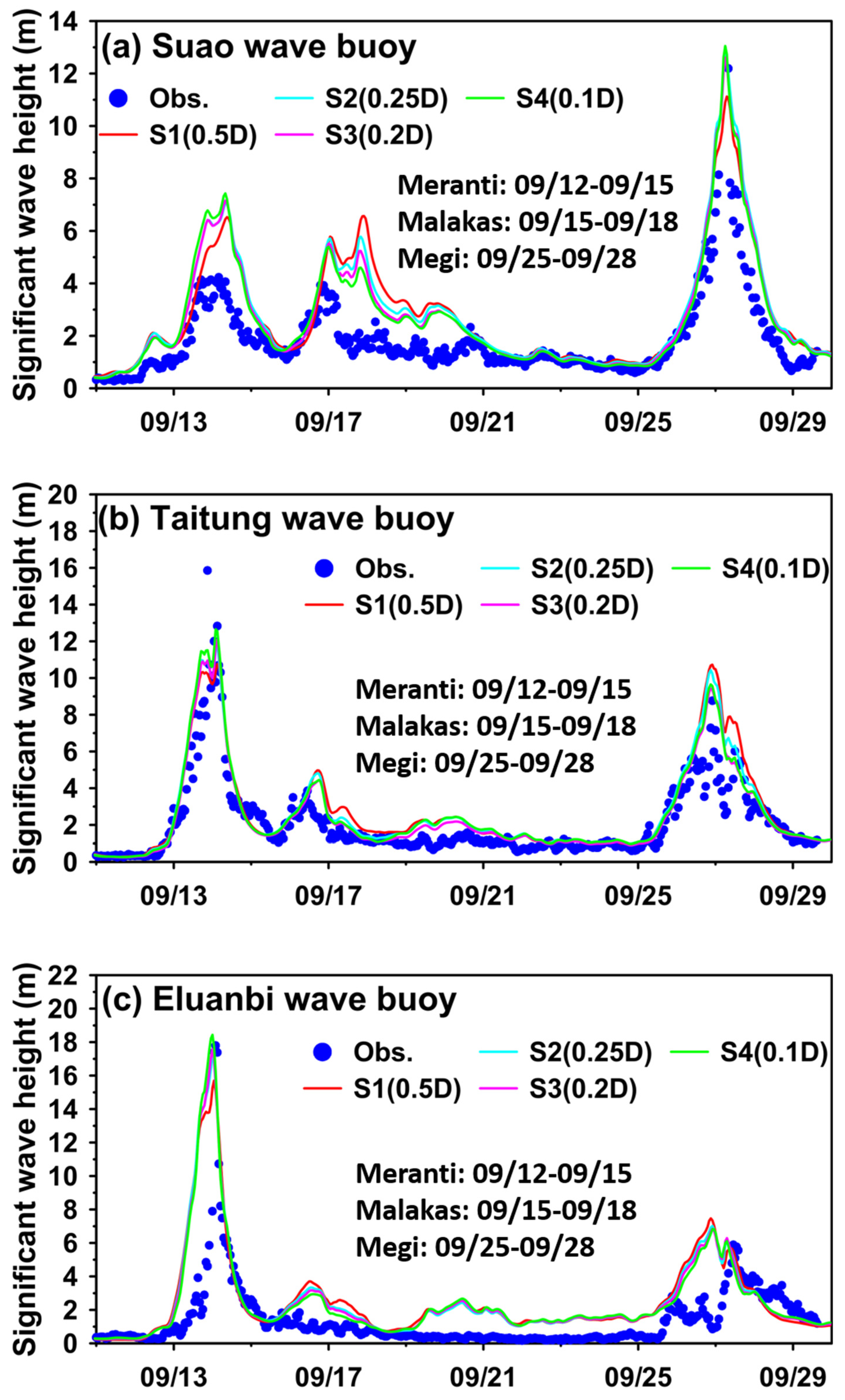
3.1. Measurements at Wave Buoys
3.2. Wind Data Input for the Wind–Wave Model
3.3. Bathymetric Data Input for the Wind–Wave Model
3.4. Wind–Wave Model Description and Configurations
4. Results
4.1. Accuracy of the Ocean Wave Simulation: Contribution of Wind Input
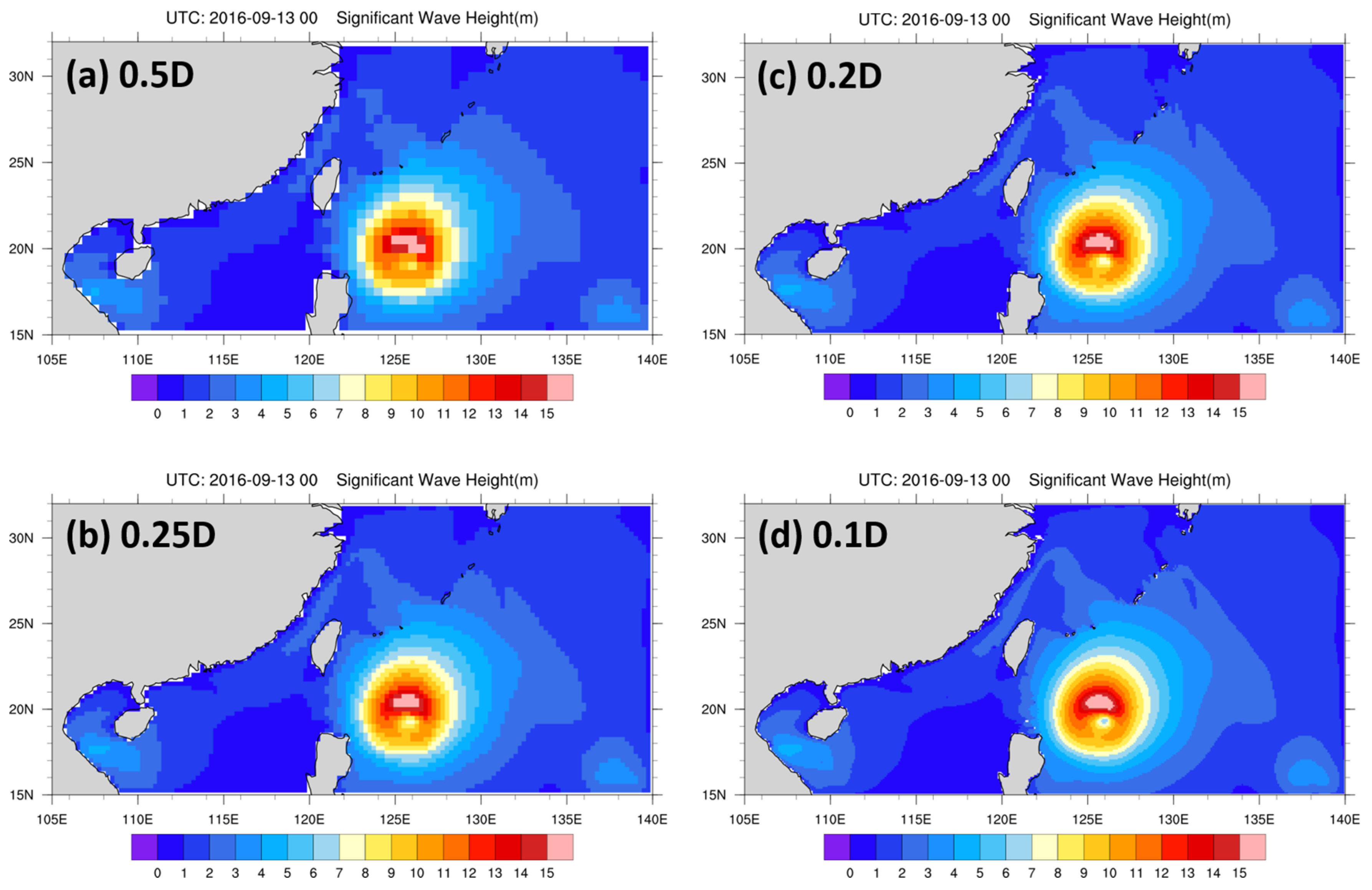
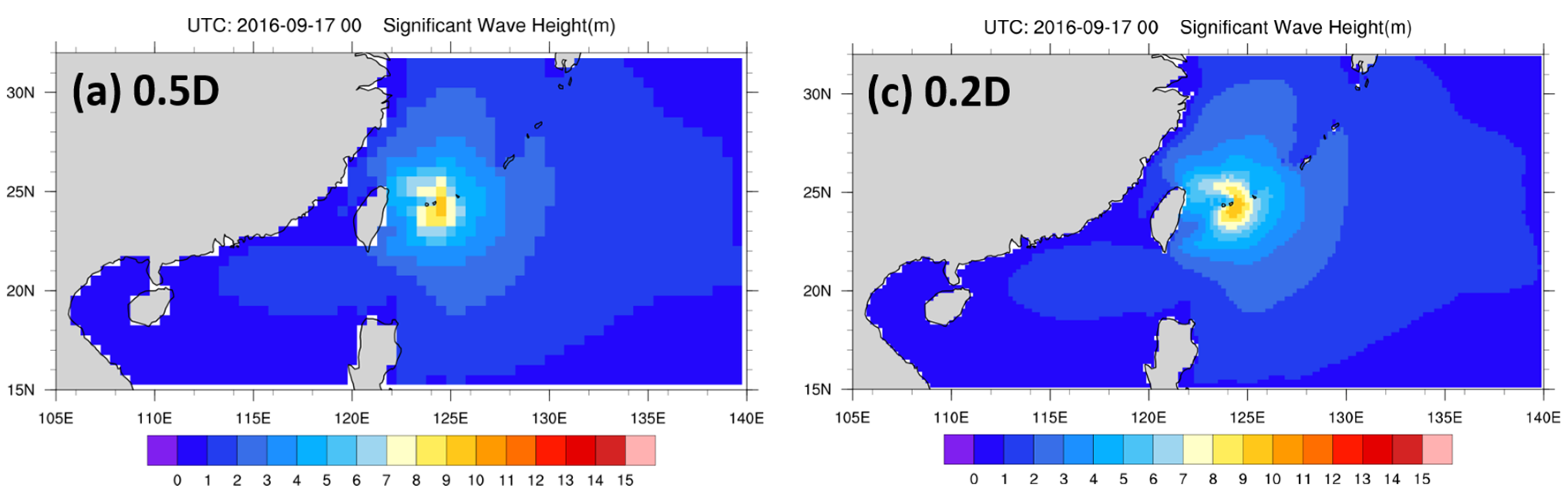
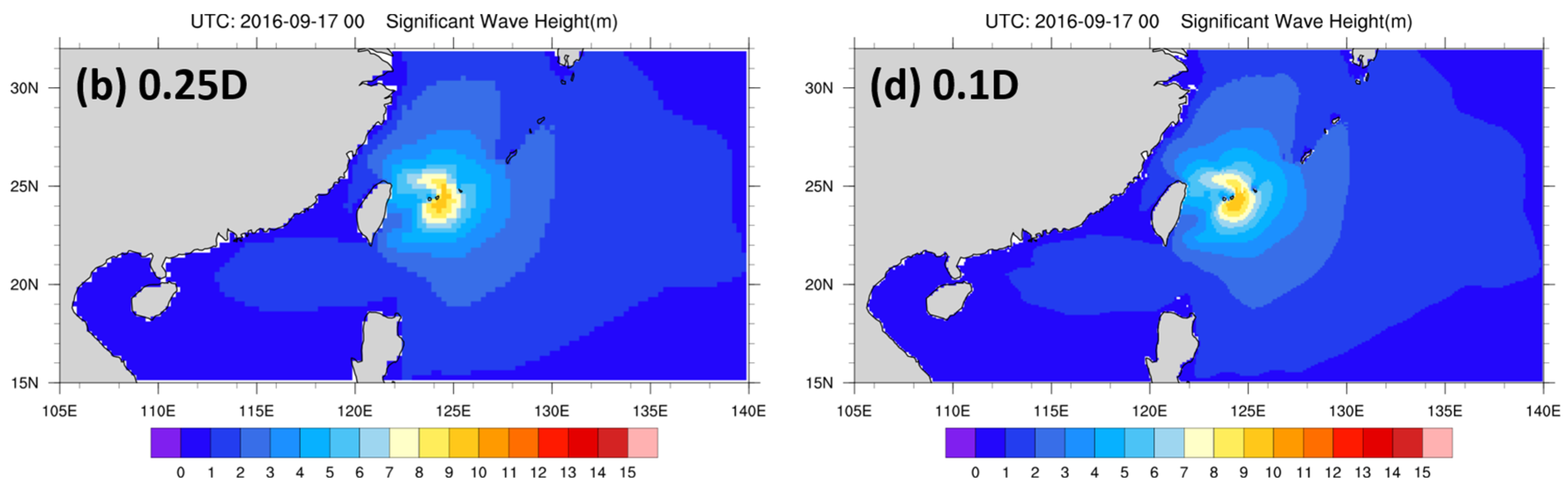
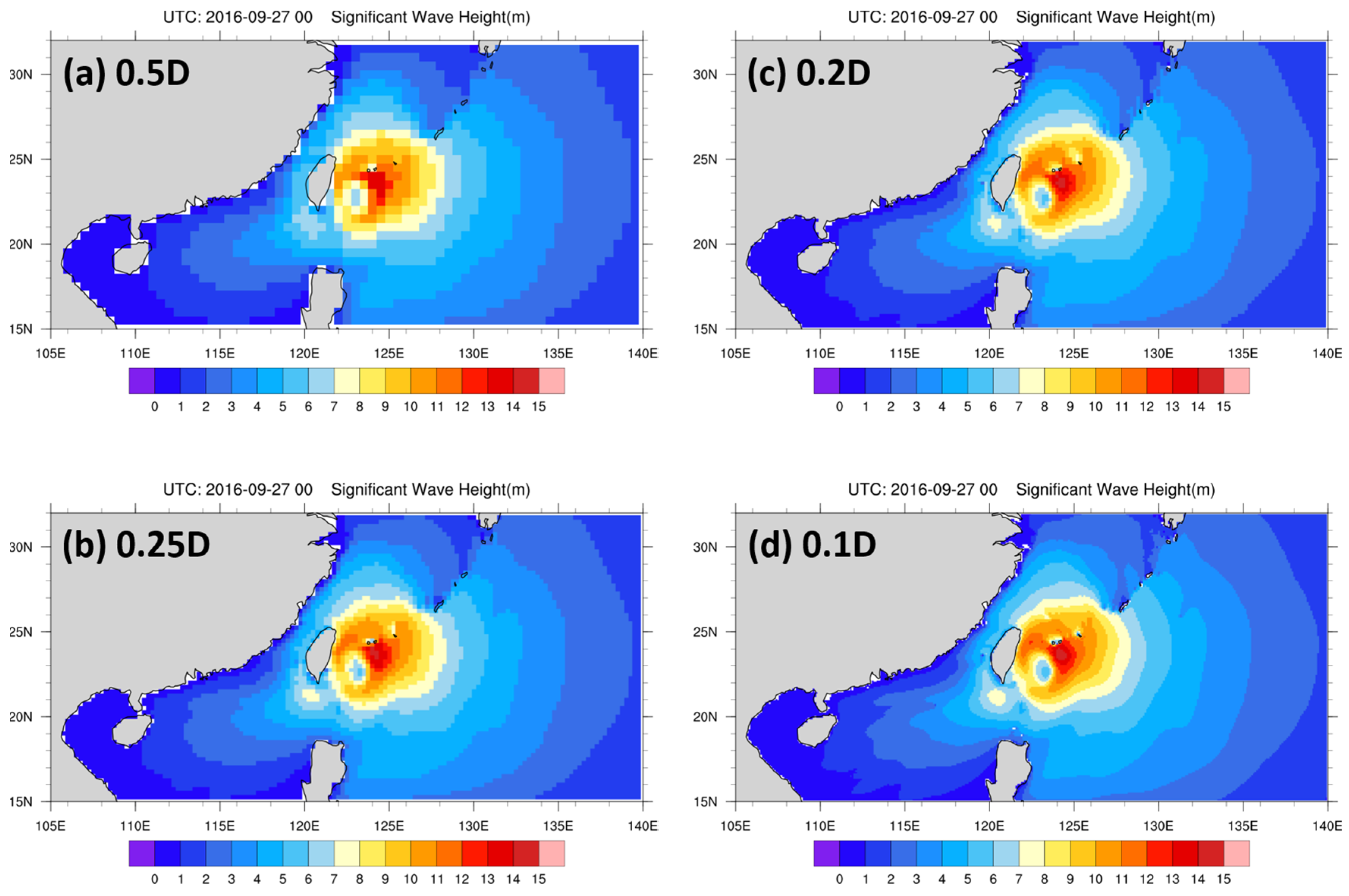
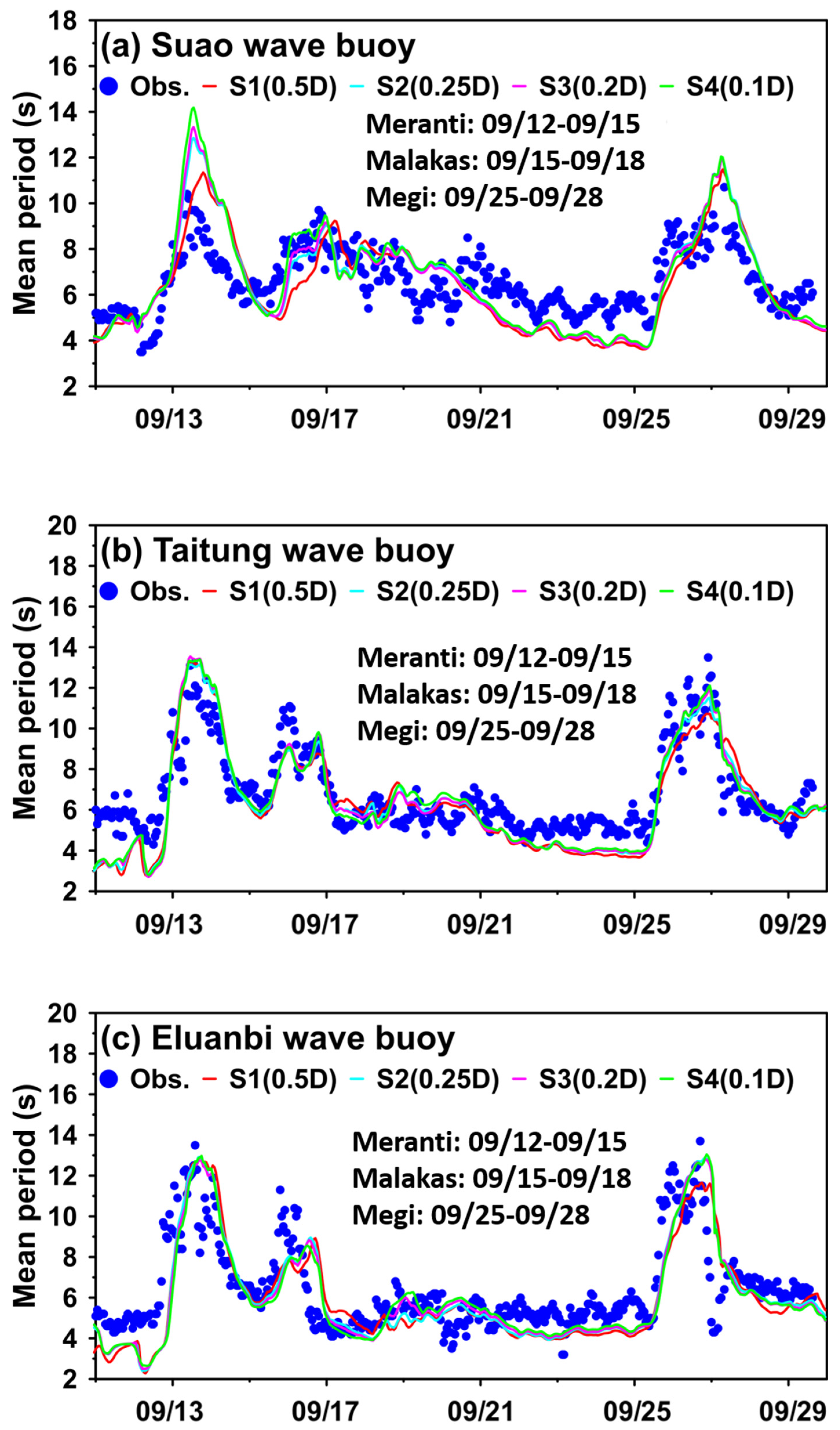
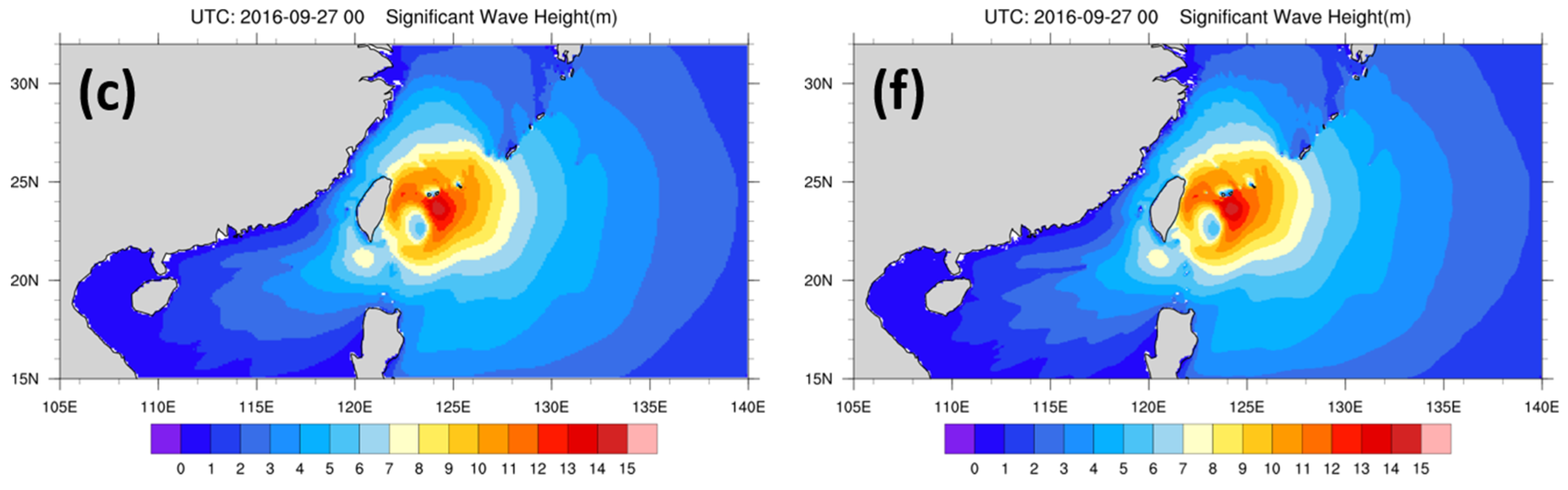
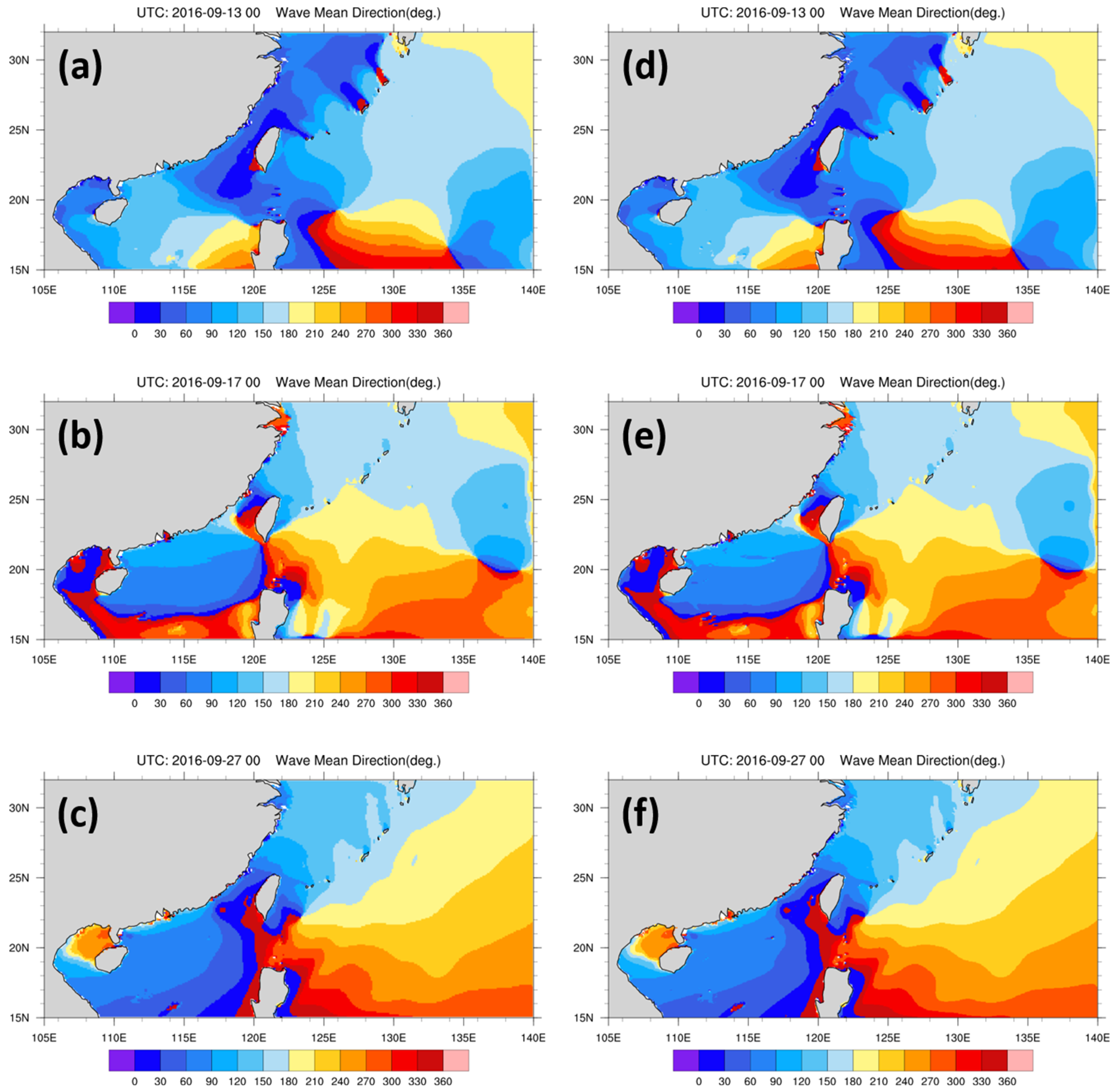
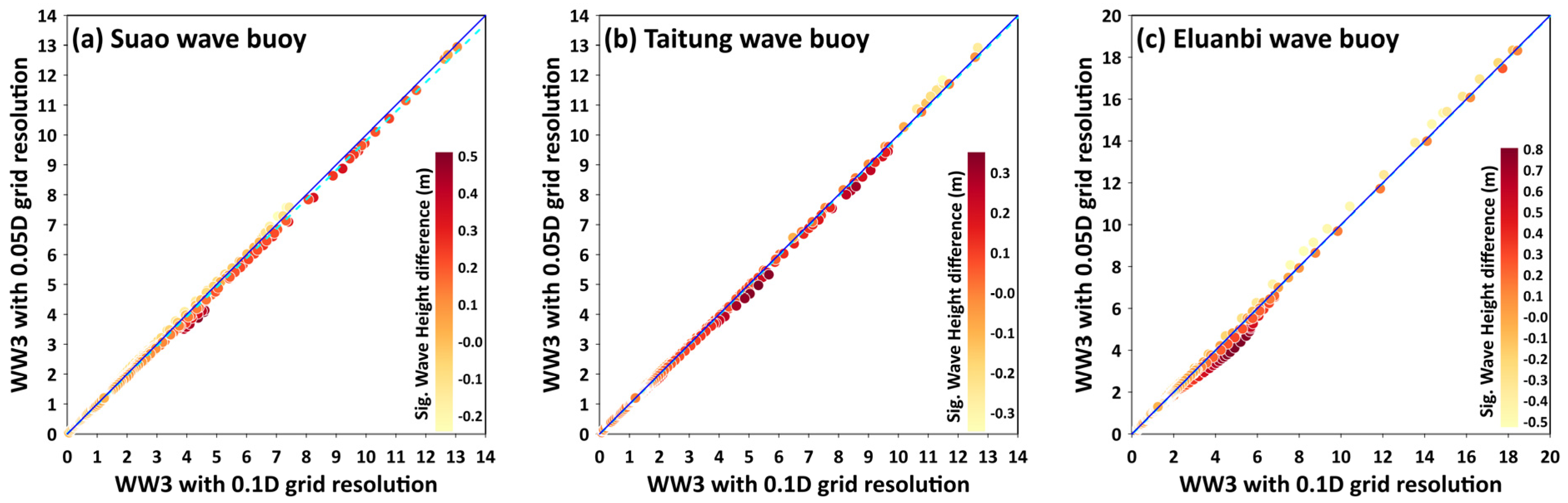
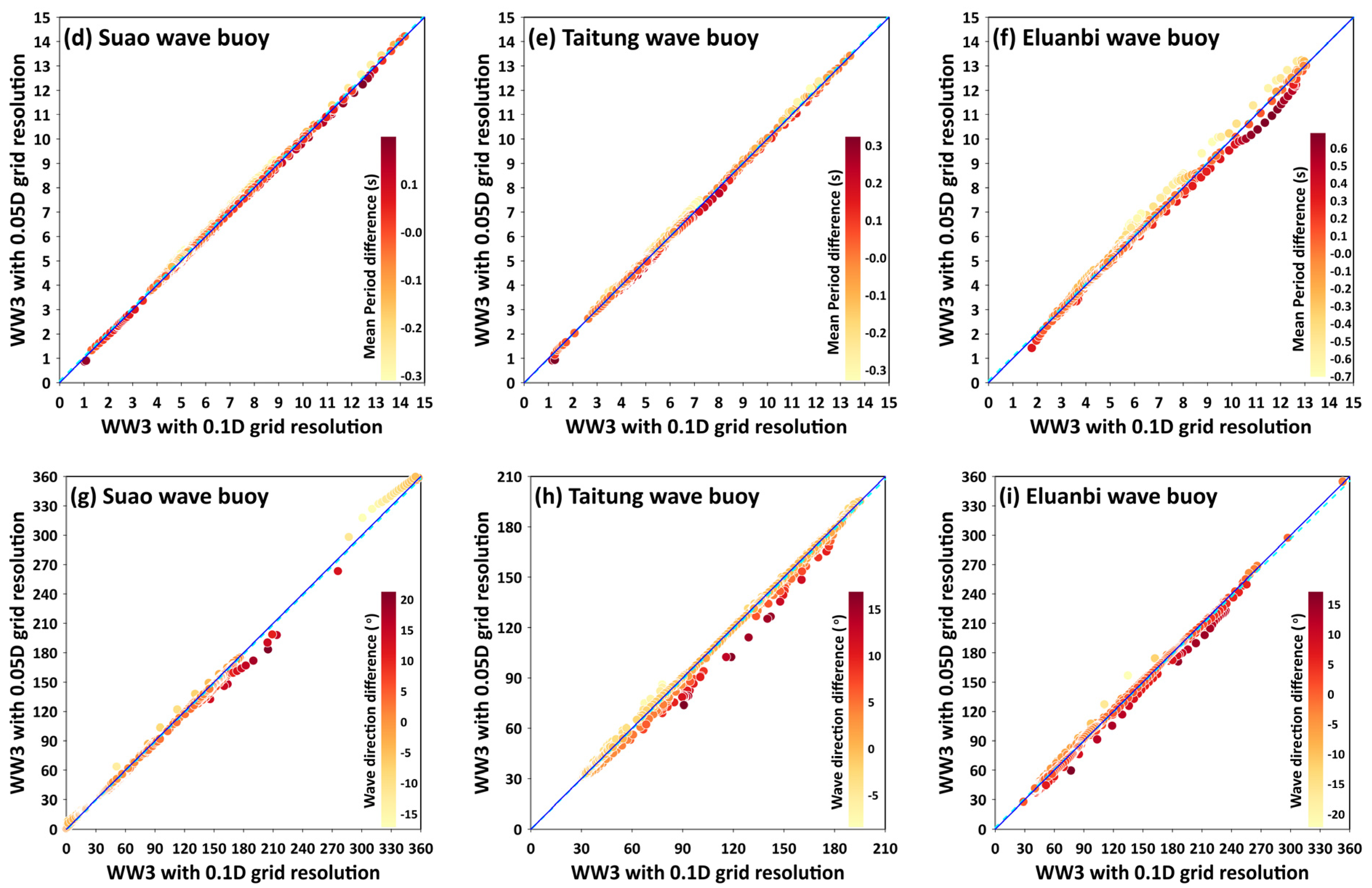
4.2. Accuracy of the Ocean Wave Simulation: Contributions of the Model Grid Resolutions
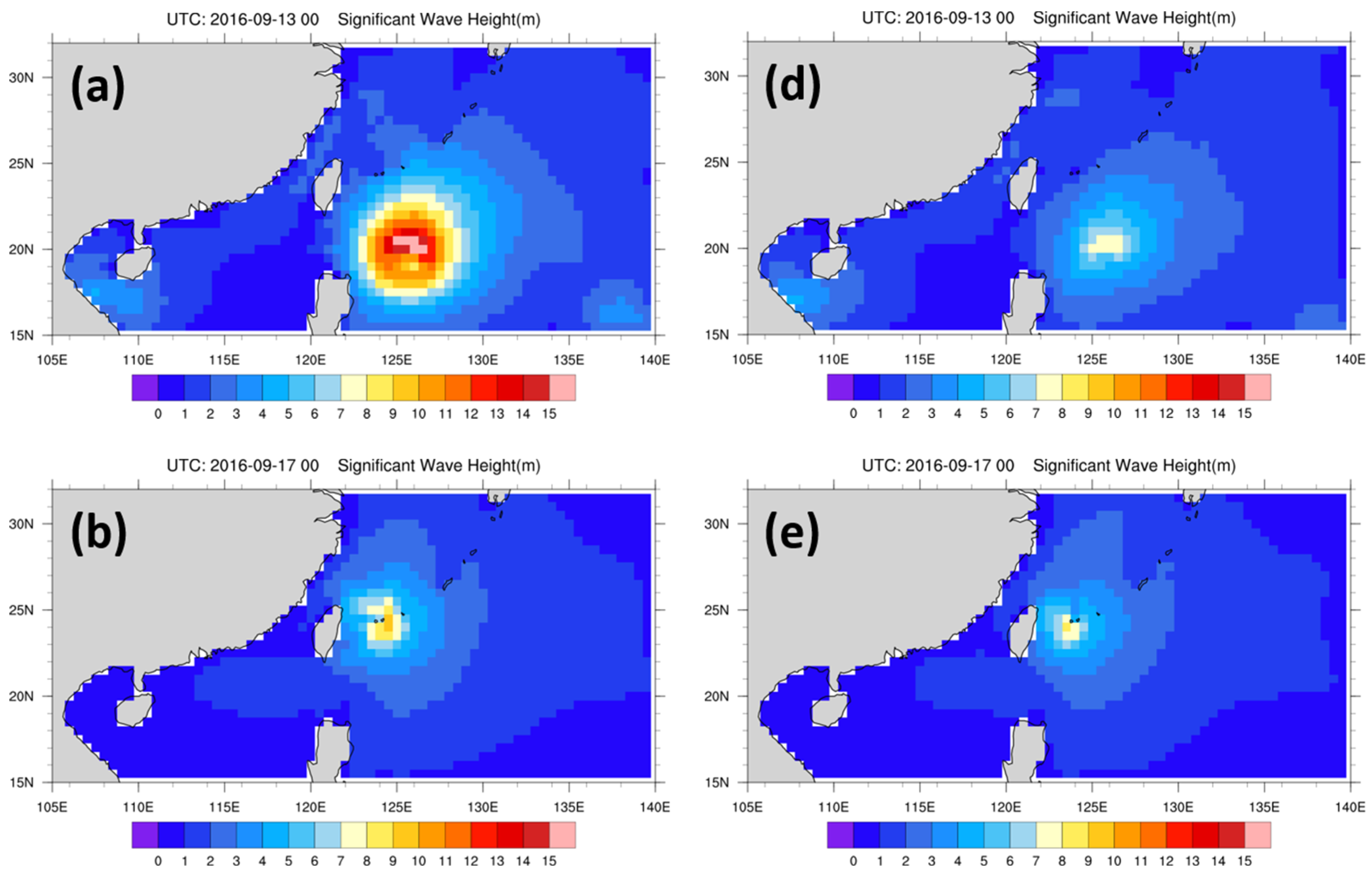
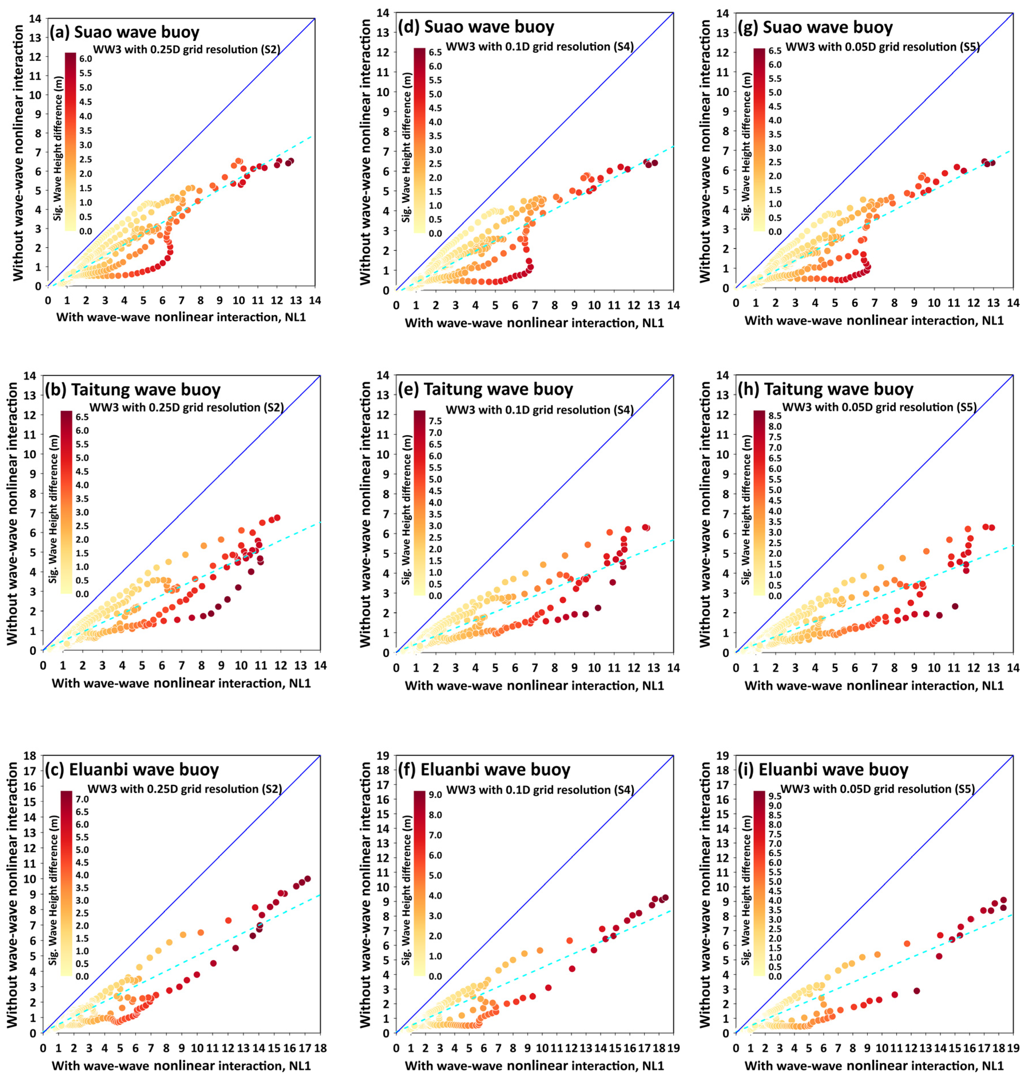
4.3. Accuracy of the Ocean Wave Simulation: Contribution of the Nonlinear Interactions
5. Discussion
5.1. Accuracy of the Ocean Wave Simulation: Contribution of the Nonlinear Interactions
5.2. Intercomparison of the WW3 and WWM-III Models for Typhoon Wave Simulations
6. Summary and Conclusions
Author Contributions
Funding
Institutional Review Board Statement
Informed Consent Statement
Data Availability Statement
Acknowledgments
Conflicts of Interest
References
- Balaguru, K.; Foltz, G.R.; Leung, L.R.; Emanuel, K.A. Global warming-induced upper-ocean freshening and the intensification of super typhoons. Nat. Commun. 2016, 7, 13670. [Google Scholar] [CrossRef] [PubMed] [Green Version]
- Chang, T.-Y.; Chen, H.; Hsiao, S.-C.; Wu, H.-L.; Chen, W.-B. Numerical Analysis of the Effect of Binary Typhoons on Ocean Surface Waves in Waters Surrounding Taiwan. Front. Mar. Sci. 2021, 8, 749185. [Google Scholar] [CrossRef]
- Chang, C.-H.; Shih, H.-J.; Chen, W.-B.; Su, W.-R.; Lin, L.-Y.; Yu, Y.-C.; Jang, J.-H. Hazard Assessment of Typhoon-Driven Storm Waves in the Nearshore Waters of Taiwan. Water 2018, 10, 926. [Google Scholar] [CrossRef] [Green Version]
- Chen, W.-B.; Chen, H.; Hsiao, S.-C.; Chang, C.-H.; Lin, L.-Y. Wind forcing effect on hindcasting of typhoon-driven extreme waves. Ocean Eng. 2019, 188, 106260. [Google Scholar] [CrossRef]
- Hsiao, S.-C.; Chen, H.; Wu, H.-L.; Chen, W.-B.; Chang, C.-H.; Guo, W.-D.; Chen, Y.-M.; Lin, L.-Y. Numerical Simulation of Large Wave Heights from Super Typhoon Nepartak (2016) in the Eastern Waters of Taiwan. J. Mar. Sci. Eng. 2020, 8, 217. [Google Scholar] [CrossRef] [Green Version]
- Hsiao, S.-C.; Wu, H.-L.; Chen, W.-B.; Chang, C.-H.; Lin, L.-Y. On the Sensitivity of Typhoon Wave Simulations to Tidal Elevation and Current. J. Mar. Sci. Eng. 2020, 8, 731. [Google Scholar] [CrossRef]
- Hsiao, S.-C.; Wu, H.-L.; Chen, W.-B.; Guo, W.-D.; Chang, C.-H.; Su, W.-R. Effect of Depth-Induced Breaking on Wind Wave Simulations in Shallow Nearshore Waters off Northern Taiwan during the Passage of Two Super Typhoons. J. Mar. Sci. Eng. 2021, 9, 706. [Google Scholar] [CrossRef]
- Shao, Z.; Liang, B.; Li, H.; Wu, G.; Wu, Z. Blended wind fields for wave modeling of tropical cyclones in the South China Sea and East China Sea. Appl. Ocean Res. 2018, 71, 20–33. [Google Scholar] [CrossRef]
- Shih, H.-J.; Chen, H.; Liang, T.-Y.; Fu, H.-S.; Chang, C.-H.; Chen, W.-B.; Su, W.-R.; Lin, L.-Y. Generating potential risk maps for typhoon-induced waves along the coast of Taiwan. Ocean Eng. 2018, 163, 1–14. [Google Scholar] [CrossRef]
- Liang, T.-Y.; Chang, C.-H.; Hsiao, S.-C.; Huang, W.-P.; Chang, T.-Y.; Guo, W.-D.; Liu, C.-H.; Ho, J.-Y.; Chen, W.-B. On-Site Investigations of Coastal Erosion and Accretion for the Northeast of Taiwan. J. Mar. Sci. Eng. 2022, 10, 282. [Google Scholar] [CrossRef]
- Choi, Y.; Cha, D.; Lee, M.; Kim, J.; Jin, C.; Park, S.; Joh, M. Satellite radiance data assimilation for binary tropical cyclone cases over the western North Pacific. J. Adv. Model. Earth Syst. 2017, 9, 832–853. [Google Scholar] [CrossRef]
- Jang, W.; Chun, H.-Y. Characteristics of Binary Tropical Cyclones Observed in the Western North Pacific for 62 Years (1951–2012). Mon. Weather. Rev. 2015, 143, 1749–1761. [Google Scholar] [CrossRef]
- Khain, A.; Ginis, I.; Falkovich, A.; Frumin, M. Interaction of binary tropical cyclones in a coupled tropical cyclone-ocean model. J. Geophys. Res. Atmos. 2000, 105, 22337–22354. [Google Scholar] [CrossRef]
- Wu, X.; Fei, J.; Huang, X.; Zhang, X.; Cheng, X.; Ren, J. A numerical study of the interaction between two simultaneous storms: Goni and Morakot in September 2009. Adv. Atmos. Sci. 2012, 29, 561–574. [Google Scholar] [CrossRef]
- Yang, C.-C.; Wu, C.-C.; Chou, K.-H.; Lee, C.-Y. Binary Interaction between Typhoons Fengshen (2002) and Fungwong (2002) Based on the Potential Vorticity Diagnosis. Mon. Weather. Rev. 2008, 136, 4593–4611. [Google Scholar] [CrossRef] [Green Version]
- Cavaleri, L.; Alves, J.-H.; Ardhuin, F.; Babanin, A.; Banner, M.; Belibassakis, K.; Benoit, M.; Donelan, M.; Groeneweg, J.; Herbers, T.; et al. Wave modelling–The state of the art. Prog. Oceanogr. 2007, 75, 603–674. [Google Scholar] [CrossRef] [Green Version]
- Abdolali, A.; Van Der Westhuysen, A.; Ma, Z.; Mehra, A.; Roland, A.; Moghimi, S. Evaluating the accuracy and uncertainty of atmospheric and wave model hindcasts during severe events using model ensembles. Ocean Dyn. 2021, 71, 217–235. [Google Scholar] [CrossRef]
- Powell, M.D.; Murillo, S.; Dodge, P.; Uhlhorn, E.; Gamache, J.; Cardone, V.; Cox, A.; Otero, S.; Carrasco, N.; Annane, B.; et al. Reconstruction of Hurricane Katrina’s wind fields for storm surge and wave hindcasting. Ocean Eng. 2010, 37, 26–36. [Google Scholar] [CrossRef]
- WAMDI Group. The WAM model- A third generation ocean wave prediction model. J. Phys. Oceanogr. 1988, 18, 1775–1810. [Google Scholar] [CrossRef]
- Tolman, H.L.; Balasubramaniyan, B.; Burroughs, L.D.; Chalikov, D.V.; Chao, Y.Y.; Chen, H.S.; Gerald, V.M. Development and implementation of wind generated ocean surface wave models at NCEP. Weather Forecast. 2002, 17, 311–333. [Google Scholar] [CrossRef]
- Booij, N.; Ris, R.C.; Holthuijsen, L.H. A third-generation wave model for coastal regions: 1. Model description and validation. J. Geophys. Res. Oceans 1999, 104, 7649–7666. [Google Scholar] [CrossRef] [Green Version]
- Roland, A.; Zhang, Y.J.; Wang, H.V.; Meng, Y.; Teng, Y.-C.; Maderich, V.; Brovchenko, I.; Dutour-Sikiric, M.; Zanke, U. A fully coupled 3D wave-current interaction model on unstructured grids. J. Geophys. Res. Oceans 2012, 117, C00J33. [Google Scholar] [CrossRef] [Green Version]
- Umesh, P.; Swain, J.; Balchand, A. Inter-comparison of WAM and WAVEWATCH-III in the North Indian Ocean using ERA-40 and QuikSCAT/NCEP blended winds. Ocean Eng. 2018, 164, 298–321. [Google Scholar] [CrossRef]
- Hersbach, H.; Bell, B.; Berrisford, P.; Hirahara, S.; Horanyi, A.; Muñoz-Sabater, J.; Nicolas, J.; Peubey, C.; Radu, R.; Schepers, D.; et al. The ERA5 global reanalysis. Q. J. R. Meteorol. Soc. 2020, 146, 1999–2049. [Google Scholar] [CrossRef]
- Saha, S.; Moorthi, S.; Wu, X.; Wang, J.; Nadiga, S.; Tripp, P.; Behringer, D.; Hou, Y.-T.; Chuang, H.-Y.; Iredell, M.; et al. The NCEP Climate Forecast System Version 2. J. Clim. 2014, 27, 2185–2208. [Google Scholar] [CrossRef]
- GEBCO Compilation Group. GEBCO 2022 Grid; GEBCO Compilation Group: Liverpool, UK, 2022. [Google Scholar] [CrossRef]
- WW3DG. User Manual and System Documentation of WAVEWATCH III Version 6.07, The WAVEWATCH III Development Group. Tech. Note 326 Pp. + Appendices, NOAA/NWS/NCEP/MMAB. 2019. College Park, MD, USA. Available online: https://www.researchgate.net/publication/336069899_User_manual_and_system_documentation_of_WAVEWATCH_III_R_version_607 (accessed on 19 March 2023).
- Abdolali, A.; Roland, A.; van der Westhuysen, A.; Meixner, J.; Chawla, A.; Hesser, T.J.; Smith, J.M.; Sikiric, M.D. Large-scale hurricane modeling using domain decomposition parallelization and implicit scheme implemented in WAVEWATCH III wave model. Coast. Eng. 2020, 157, 103656. [Google Scholar] [CrossRef]
- Chen, W.-B. Typhoon Wave Simulation Responses to Various Reanalysis Wind Fields and Computational Domain Sizes. J. Mar. Sci. Eng. 2022, 10, 1360. [Google Scholar] [CrossRef]
- Ardhuin, F.; Rogers, E.; Babanin, A.V.; Filipot, J.-F.; Magne, R.; Roland, A.; Van Der Westhuysen, A.; Queffeulou, P.; Lefevre, J.-M.; Aouf, L.; et al. Semiempirical Dissipation Source Functions for Ocean Waves. Part I: Definition, Calibration, and Validation. J. Phys. Oceanogr. 2010, 40, 1917–1941. [Google Scholar] [CrossRef] [Green Version]
- Hasselmann, K.; Barnett, T.P.; Bouws, E.; Carlson, H.; Cartwright, D.E.; Enke, K.; Ewing, J.A.; Gienapp, H.; Hasselmann, D.E.; Kruseman, P.; et al. Measurements of Wind-Wave Growth and Swell Decay during the Joint North Sea Wave Project (JONSWAP); Deutsches Hydrographisches Institut: Berlin/Hamburg, Germany, 1973; Available online: https://repository.tudelft.nl/islandora/object/uuid%3Af204e188-13b9-49d8-a6dc-4fb7c20562fc (accessed on 19 March 2023).
- Battjes, J.A.; Janssen, J.P.F.M. Energy loss and set-up due to breaking of random waves. Coast. Eng. Proc. 1978, 1, 32. [Google Scholar] [CrossRef] [Green Version]
- Tolman, H.L. Inverse modeling of discrete interaction approximations for nonlinear interactions in wind waves. Ocean Model. 2004, 6, 405–422. [Google Scholar] [CrossRef]
- Monteiro, N.M.; Oliveira, T.C.; Silva, P.A.; Abdolali, A. Wind–wave characterization and modeling in the Azores Archipelago. Ocean Eng. 2022, 263, 112395. [Google Scholar] [CrossRef]
- Holthuijsen, L.H. Waves in Oceanic and Coastal Waters; Cambridge University Press (CUP): Cambridge, UK, 2007. [Google Scholar] [CrossRef]
- Hasselmann, S.; Hasselmann, K.; Allender, J.H.; Barnett, T.P. Computations and parameterizations of the nonlinear energy transfer in a gravity-wave spectrum, Part II: Parameterizations of the nonlinear energy transfer for application in wave models. J. Phys. Oceanogr. 1985, 15, 1378–1391. [Google Scholar] [CrossRef]
- Tolman, H.L. A Generalized Multiple Discrete Interaction Approximation for resonant four-wave interactions in wind wave models. Ocean Model. 2013, 70, 11–24. [Google Scholar] [CrossRef]
- Su, W.-R.; Chen, H.; Chen, W.-B.; Chang, C.-H.; Lin, L.-Y.; Jang, J.-H.; Yu, Y.-C. Numerical investigation of wave energy resources and hotspots in the surrounding waters of Taiwan. Renew. Energy 2018, 118, 814–824. [Google Scholar] [CrossRef]
- Hsiao, S.-C.; Chen, H.; Chen, W.-B.; Chang, C.-H.; Lin, L.-Y. Quantifying the contribution of nonlinear interactions to storm tide simulations during a super typhoon event. Ocean Eng. 2019, 194, 106661. [Google Scholar] [CrossRef]
- Yu, Y.-C.; Chen, H.; Shih, H.-J.; Chang, C.-H.; Hsiao, S.-C.; Chen, W.-B.; Chen, Y.-M.; Su, W.-R.; Lin, L.-Y. Assessing the Potential Highest Storm Tide Hazard in Taiwan Based on 40-Year Historical Typhoon Surge Hindcasting. Atmosphere 2019, 10, 346. [Google Scholar] [CrossRef] [Green Version]


| Model Configuration | Scenarios | ||||
|---|---|---|---|---|---|
| S1 | S2 | S3 | S4 | S5 | |
| Mesh resolution | 0.50 deg | 0.25 deg | 0.20 deg | 0.10 deg | 0.05 deg |
| Number of grid points | 2485 | 9729 | 15,136 | 60,021 | 239,041 |
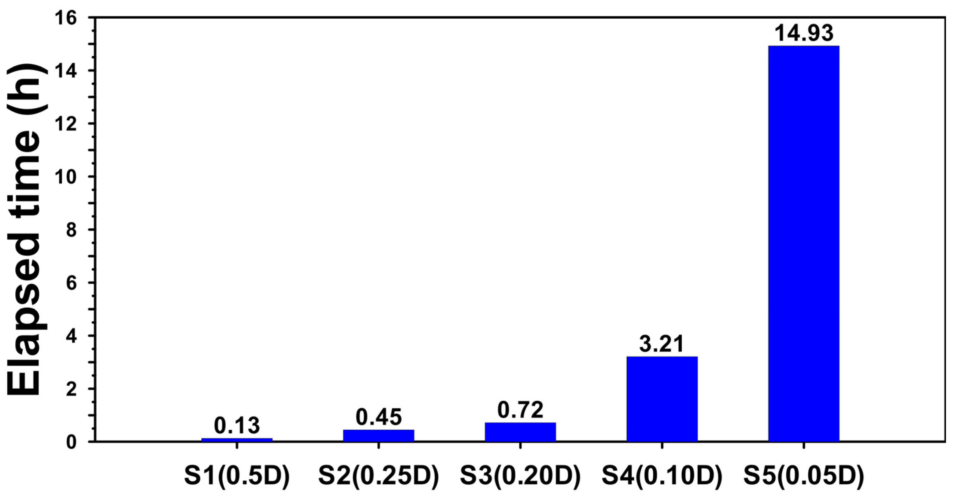
| Elapsed time of a 29-day simulation | 0.13 h | 0.45 h | 0.72 h | 3.21 h | 14.93 h |
| Parameters | Value or Package |
|---|---|
| Time step | 180 s |
| Number of direction bins | 36 |
| Number of frequencies | 36 |
| Source term | ST4, Ref. [30] source term package |
| Wave bottom dissipation | BT1 [31], JONSWAP bottom friction formulation |
| Depth-induced wave breaking | DB1, Ref. [32] Battjes–Janssen module |
| Nonlinear wave–wave interactions | NL1 [33], discrete interaction approximation |
Disclaimer/Publisher’s Note: The statements, opinions and data contained in all publications are solely those of the individual author(s) and contributor(s) and not of MDPI and/or the editor(s). MDPI and/or the editor(s) disclaim responsibility for any injury to people or property resulting from any ideas, methods, instructions or products referred to in the content. |
© 2023 by the authors. Licensee MDPI, Basel, Switzerland. This article is an open access article distributed under the terms and conditions of the Creative Commons Attribution (CC BY) license (https://creativecommons.org/licenses/by/4.0/).
Share and Cite
Hsiao, S.-C.; Wu, H.-L.; Chen, W.-B. Study of the Optimal Grid Resolution and Effect of Wave–Wave Interaction during Simulation of Extreme Waves Induced by Three Ensuing Typhoons. J. Mar. Sci. Eng. 2023, 11, 653. https://doi.org/10.3390/jmse11030653
Hsiao S-C, Wu H-L, Chen W-B. Study of the Optimal Grid Resolution and Effect of Wave–Wave Interaction during Simulation of Extreme Waves Induced by Three Ensuing Typhoons. Journal of Marine Science and Engineering. 2023; 11(3):653. https://doi.org/10.3390/jmse11030653
Chicago/Turabian StyleHsiao, Shih-Chun, Han-Lun Wu, and Wei-Bo Chen. 2023. "Study of the Optimal Grid Resolution and Effect of Wave–Wave Interaction during Simulation of Extreme Waves Induced by Three Ensuing Typhoons" Journal of Marine Science and Engineering 11, no. 3: 653. https://doi.org/10.3390/jmse11030653