An Improved Method for Optimizing CNC Laser Cutting Paths for Ship Hull Components with Thicknesses up to 24 mm

Abstract

In this paper, the essence and optimization objectives of the hull parts path optimization problem of CNC laser cutting are described, and the shortcomings of the existing optimization methods are pointed out. Based on the optimization problem of the hull parts CNC laser cutting path, a new part-cutting constraint rule based on partial cutting is proposed, which aims to overcome the drawbacks of the traditional algorithms with serial cutting constraint rules. This paper addresses the problem of optimizing the path for CNC laser cutting of hull parts, including an empty path and the order and directions used for the provided cut contours. Based on the discretization of the part contour segments, a novel toolpath model for hull parts called hull parts cutting path optimization problems based on partial cutting rules (HPCPO) is proposed in this paper. To solve the HPCPO problem, a segmented genetic algorithm based on reinforcement learning (RLSGA) is proposed. In RLSGA, the population is viewed as an intelligent agent, and the agent’s state is the population’s diversity coefficient. Three different segmented crossover operators are considered as the agent’s actions, and the agent’s reward is related to the changes in the population’s fitness and diversity coefficients. Two benchmark problems for HPCPO were constructed to evaluate the performance of RLSGA and compared with four other algorithms. The results showed that RLSGA outperformed the other algorithms and effectively solved the HPCPO problem.

1. Introduction

Shipbuilding is an intricate and specialized industry where the manufacturing process’s efficiency and accuracy significantly impact the final product’s quality and cost-effectiveness [1]. In recent years, with the continuous advancement of manufacturing technology, computer numerical control (CNC) laser cutting has become a commonly used method for metal material processing in modern manufacturing. 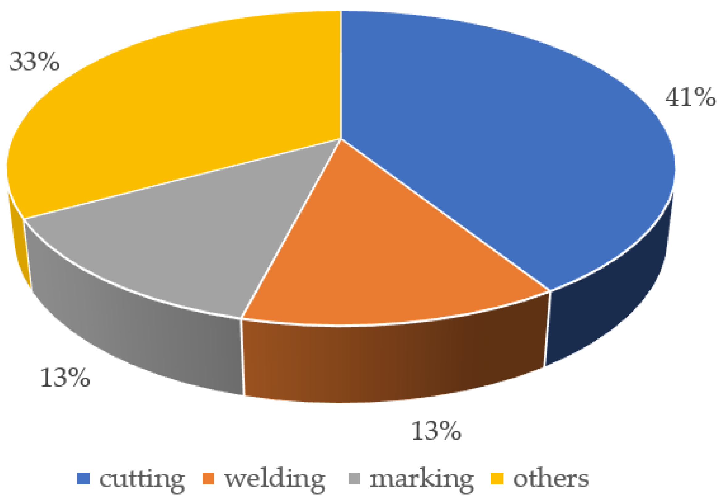The CNC laser cutting computer-aided manufacturing system provides significant benefits such as shortened product development cycles, improved production efficiency, enhanced product quality, and reduced energy consumption [2]. According to the “2021 China Laser Industry Development Report,” laser cutting has the most significant proportion in the laser industry’s actual application, followed by laser welding and laser marking, as illustrated in Figure 1. CNC laser cutting technology has become a vital tool in the shipbuilding industry, capable of accurately and efficiently cutting various hull components, including the hull plate, bulkheads, and decks [3]. As a critical technology in laser cutting systems, automatic nesting and cutting path planning have received increasing attention from research units and scholars [4].

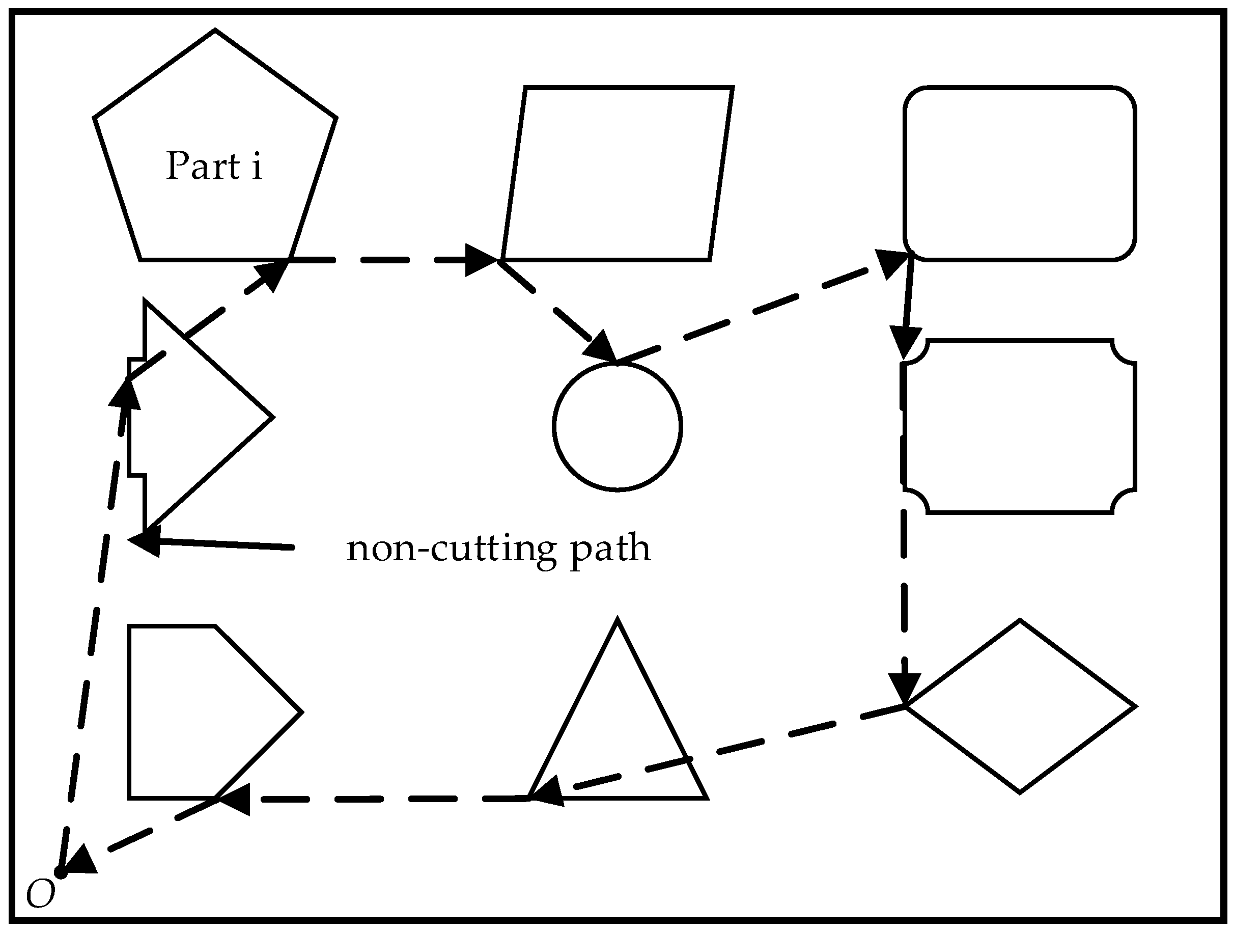
For flat laser cutting, the travel path of the laser head consists of the processing trajectory and the auxiliary processing path. The processing trajectory refers to the laser head’s travel path as it cuts the graphic outline. In contrast, the auxiliary processing path, the non-cutting path, represents the laser head’s movement path between different graphic outlines. The auxiliary processing path serves the critical function of quickly and accurately positioning the laser head, determining the cutting order of various outlines, and improving processing efficiency. Figure 2 illustrates the schematic diagram of the laser head non-cutting path.

This paper focuses on optimizing the non-cutting path for laser cutting, which involves finding the optimal path for the laser head movement based on the requirements of the cutting process in a prenested layout [5]. The size of the non-cutting path is related to the cutting order and the starting processing point. Reducing the non-cutting path and avoiding unnecessary movement of the laser head can significantly improve the efficiency of parts with complex trajectories, especially those with batch production requirements.

Laser cutting has higher production requirements and costs than wire, waterjet, and plasma. Therefore, reducing the size of the non-cutting path is essential in decreasing operating costs, conserving resources, and improving production efficiency. For instance, the cost analysis of ${\mathrm{CO}}_2$ laser and fiber laser cutting processes for cutting a 5 mm stainless steel plate is shown in

Table 1. CO₂ laser and fiber laser cutting process cost analysis.

Classification		Consumption
		CO2 Laser	Fiber Laser
laser gas consumption	$\mathrm{He}(99.999\%)/\mathrm{L}\cdot {\mathrm{h}}^{-1}$	13	-
	${\mathrm{N}}_2(99.999\%)/\mathrm{L}\cdot {\mathrm{h}}^{-1}$	6	-
	${\mathrm{CO}}_2(99.999\%)/\mathrm{L}\cdot {\mathrm{h}}^{-1}$	1	-
	$\mathrm{Compressed}\hspace{0.17em}{\mathrm{air}/\mathrm{Nm}}^3\cdot {\mathrm{h}}^{-1}$	- 2	35
cutting gas consumption	$\mathrm{Cutting}\hspace{0.17em}\mathrm{speed}/\mathrm{m}\cdot {\min }^{-1}$	2.5	8.2
	${\mathrm{N}}_2(99{.999\%)/\mathrm{Nm}}^3\cdot {\mathrm{h}}^{-1}$	20.27	39.25
Electricity consumption	$\mathrm{Total}\mathrm{power}\mathrm{of}\mathrm{equipment}/\mathrm{kW}$	47.56	28.56
equipment depreciation	Total purchase and installation cost/¥$\cdot \mathrm{Y}$	650,000	700,000
equipment maintenance	Equipment repair and maintenance costs/¥$\cdot \mathrm{Y}$ 1	100,000	70,000
Vulnerable and consumable parts consumption	Focusing lens/piece$\cdot \mathrm{Y}$	belike 4	-
	Protective lens/day$\cdot \mathrm{Y}$	-	2.5
	Nozzle/h$\cdot {\mathrm{piece}}^{-1}$	40	40
	Other consumption/¥$\cdot \mathrm{Y}$	belike 4000	belike 4000

¹ Y stands for yearly. ² “-” indicates that this consumption is not required.

, highlighting the high cost of laser cutting. Thus, planning the cutting path is crucial to reduce production costs [6].

The remaining parts of this paper are organized as follows: Section 2 reviews the relevant literature. Section 3 provides a detailed description of the cutting path optimization problem and cutting path optimization model based on partial cutting rules. Section 4 introduces the designed RLSGA algorithm. Section 5 verifies the effectiveness and efficiency of the proposed model and algorithm through experiments. Section 6 provides further conclusions and discussions.

2. Literature Review

Madić et al. [7] proposed a genetic programming (GP) approach to develop a mathematical model that describes the CO₂ laser cutting process for the aluminum alloy AlMg3. This study used GP to investigate the relationship between cutting speed, laser power, assist gas pressure, and kerf taper angle. The authors conducted a complete factorial design experiment to obtain the GP model evolution process database. The results showed that the fit between the experimental and GP model prediction values of the kerf taper angle was appropriate. Furthermore, 3D surface plots were generated using the derived GP mathematical model to analyze the effects of input parameters on the change in kerf taper angle values. This study demonstrated the potential of GP in developing empirical mathematical models for laser cutting process optimization. Sherif et al. [8] proposed a two-stage sequential optimization approach in laser cutting for the nesting and cutting sequence. The paper focuses on developing a solution technique for any layout’s optimal cutting sequence. A simulated annealing algorithm (SAA) was considered to evolve the optimal cutting sequence. The proposed SAA was tested with five typical problems and was shown to provide near-optimal solutions. Comparing the two literature problems reveals that the proposed SAA can give improved results compared to GA and ACO algorithms. This study aims to maximize material utilization and minimize the ideal travel distance of the laser cut tool.

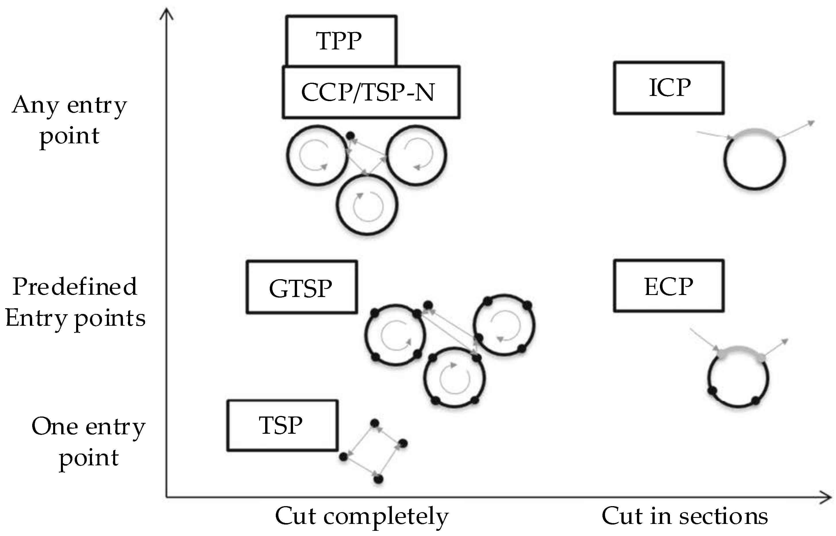
In 2016, Dewil et al. [9] classified the problem of laser cutting path planning into six categories: the continuous cutting problem (CCP), the endpoint cutting problem (ECP), the intermittent cutting problem (ICP), the touring polygons problem (TPP), the traveling salesman problem (TSP), and the generalized traveling salesman problem (GTSP). Each problem differs in selecting start and end points for the machining trajectory and in whether the graphic contour must be entirely cut. Various methods have been proposed to address each problem. Figure 3 shows the classification of the problems and their relationships. Currently, most scholars simplify the cutting path planning problem into two categories: the traveling salesman problem model and the generalized traveling salesman problem model. They have proposed a range of optimization algorithms to solve these two categories of problems.

Establishing a mathematical model for the traveling salesman problem (TSP) and utilizing intelligent optimization algorithms to solve the laser cutting path planning problem is a common approach. Shen Lu [10] proposed two heuristic search algorithms, namely the “n”-shaped and “s”-shaped algorithms. These algorithms simplify the shape center of each city point and use a centroid genetic algorithm to solve the traveling salesman problem to obtain the sequence of the laser cutting air path. Based on the nearest principle, the characteristic points of each part are searched to determine the entry point of the laser head. To avoid the laser head passing through the already-cut area, an improved genetic algorithm is proposed to satisfy the laser cutting process requirements and minimize the air travel path. In contrast to the selection of contour control points mentioned earlier, Li Nini et al. [11] extracted a node from each closed contour to represent the entire contour, treating the laser cutting path planning as a traveling salesman problem and using an improved genetic algorithm to solve it. For non-closed contour graphics, Chen Ting et al. [12] combined the background of the laser cutting die industry and used the taboo search greedy heuristic algorithm to plan the path. To improve the global search ability of the greedy algorithm, the algorithm was optimized locally. Hu Shenghong [13] determined the processing order of the image group and the processing start point of each image group based on greedy and taboo search algorithms. Zhou Rui et al. [14] used a genetic algorithm as the framework and introduced local operators to solve the laser cutting collaborative operation path planning problem.

Compared to the traveling salesman problem, the generalized traveling salesman problem is more complex due to multiple control points in each graph. Chentsov [15] highlighted the limitations of using dynamic programming to solve such problems in the early days, as they were unable to handle large-scale data. He proposed a quasi-optimal greedy algorithm to solve this problem and compared the results of exact and approximate algorithms. Laser cutting, as a particular processing method, imposes multiple process requirements on path planning, which introduces new perspectives to researching such problems. Lin Lizong et al. [16] investigated the cutting order problem of nested contours in laser cutting, established a mathematical model of empty movement paths, added a graphic preprocessing stage, computed the minimum bounding rectangle of each contour, and used a two-level programming design genetic optimization algorithm under the laser cutting process conditions of internal cutting before external cutting for complex contour shapes and non-crossing cutting paths in the already-cut area. The contour line corner points and the boundary corner points of the bounding rectangle determine the positional relationship of the nested contour line. Considering practical processing issues such as plate heating during laser cutting, Song Lei et al. [17] formulated a multi-objective function mathematical model for laser cutting path planning. They employed a dual-chromosome genetic algorithm with a dual-chromosome coding method and suitably modified genetic algorithm steps such as crossover and mutation. To account for constraints such as “punching,” “cutting along,” and “no crossing cutting” paths, Wang Na et al. [18] established a constrained GTSP model. They utilized a bidirectional ant colony optimization algorithm to address the problem of optimizing the closed contour path. Wang Zheng et al. [19] constructed a generalized traveling salesman problem model to address the shortcut path optimization problem for multiple contours and employed a quantum evolutionary algorithm to obtain the processing sequence. Dynamic programming has the advantage of achieving the optimal decision; therefore, it is utilized to calculate individual fitness. The quantum replacement method also enhances the global search capability of the algorithm. Yang Jianjun et al. [20] proposed the concept of time distance. They utilized a dual encoding genetic algorithm to determine the contour processing sequence and the starting points of each contour while considering the thermal effect problem in laser cutting. Dewil et al. [21] viewed path planning as the division of a contour line, and the partition minimized the cost of connecting the rooted directed minimum spanning tree. They employed the Edmond–Liu algorithm to solve the tree problem and the improved Liu–Kernighan heuristic algorithm to solve the generalized traveling salesman problem. Hajad et al. [22] proposed a simulated annealing algorithm with an adaptive large neighborhood search to minimize the laser cutting path in a two-dimensional cutting process. The algorithm extracts cut profiles from the input image using image processing algorithms and assigns coordinates to the contours’ pixels. Based on the generalized traveling salesman problem, the optimization algorithm considers all input image pixels as potential piercing locations. A laser beam makes a single visit and then does a complete cut of each profile consecutively. The simulation results showed that the proposed algorithm could successfully solve several datasets from the GTSP-Lib database with good solution quality. Additionally, the cutting path generated by the proposed method was shorter than that recommended by the commercial CAM software and other previous works.

The studies mentioned above examined the problem of optimizing cutting paths from different perspectives. However, the methodologies employed are often quite similar, with most converting the problem into a TSP by applying the constraint rule of sequential cutting of parts and subsequently employing relevant algorithms for optimization and solution. Nevertheless, the constraint rule of sequential cutting significantly impacts the practical effectiveness of cutting path optimization, leading to cases where the best path found is not a truly optimal solution.

This paper’s primary focus is optimizing the numerical control laser cutting path for hull components without holes and with non-adjacent edges. Specifically, the relationship between the cutting constraints of the parts and the path of the laser head is explored, along with relevant optimization algorithms. This study addresses critical issues in optimizing hull components’ numerical control laser cutting path.

3. Problem Description and Formulation

3.1. Problem Description

As shown in Figure 4, this paper considers a scenario where $M$ parts without holes and with no common edges need to be cut from a plate. The cutting process begins at the lower left corner of the plate, denoted as the origin $O$, and the laser head cuts the contour shape of each part in turn. Finally, the laser head returns to the origin $O$ to complete all parts’ cutting and blanking processes. During the cutting process, the laser head is “laser on cutting” when moving along the part contour line and in the “laser off non cutting” state (i.e., empty travel) when moving between contours. Since the length of the part contour is fixed, minimizing the empty travel distance between contours is crucial in reducing the cutting path length when the laser head’s movement speed is constant. Therefore, cutting path optimization aims to find the optimal path for the laser head, which minimizes the empty travel distance during the cutting process.

3.2. Model Establishment

3.2.1. Part-Cutting Constraint Rules

Many current studies in this field adopt the constraint rule of serial cutting of parts, where the laser head follows the part’s contour for a complete loop before moving on to the next part. Thus, the shape of the part’s contour may need to be considered when analyzing and optimizing the cutting path. A single point is selected from the contour as the starting and ending point of the contour (cutting point), which can replace the part’s contour. Consequently, the contours of the parts to be cut can be simplified as a set of points on the plate plane, and the cutting path optimization problem can be transformed into the well-known traveling salesman problem (TSP) to find the shortest distance between point sets. Most studies initially utilize the nearest neighbor algorithm to determine the cutting points for each contour and then use various related algorithms to optimize and solve the TSP, thereby resolving the cutting path optimization problem. However, based on in-depth research, this method, while simplifying the problem, may have a specific impact on the optimization results. As shown in Figure 5a, two parts are waiting to be cut inside the sheet, with the vertices of part 1 being ($P_1^1$, $P_2^1$, $P_3^1$, $P_4^1$, $P_5^1$) and those of part 2 being ($P_1^2$, $P_2^2$, $P_3^2$, $P_4^2$). Using the nearest neighbor algorithm to determine the punching points as $P_1^1$ and $P_1^2$, the complete cutting path can be represented as:

$$O\to P_1^1\to [\hspace{0.17em}{P}_2^1\to P_3^1\to P_4^1\to P_5^1\to P_1^1\hspace{0.17em}]\to P_1^2\to [\hspace{0.17em}{P}_2^2\to P_3^2\to P_4^2\to P_1^2\hspace{0.17em}]\to O$$

The empty travel distance is $S^{\prime }=\overline{O{P}_1^1}+\overline{P_1^1{P}_1^2}+\overline{P_1^{2}O}$. If the laser head is not subject to the constraint of serial cutting, i.e., allowing it to change position to cut other parts before one part is completely cut, then the cutting path shown in Figure 5b can be obtained:

$$O\to P_1^1\to [\hspace{0.17em}{P}_2^1\to P_3^1\to P_4^1\hspace{0.17em}]\to P_1^2\to [\hspace{0.17em}{P}_2^2\to P_3^2\to P_4^2\to P_1^2\hspace{0.17em}]\to P_4^1\to [\hspace{0.17em}{P}_5^1\hspace{0.17em}\to P_1^1\hspace{0.17em}]\to O$$

The empty travel distance, in this case, is

$$S=\overline{O{P}_1^1}+\overline{P_4^1{P}_1^2}+\overline{P_1^2{P}_4^1}+\overline{P_1^{1}O}=2\overline{O{P}_1^1}+2\overline{P_4^1{P}_1^2}$$

It is clear that $S^{\prime }>S$. Hence, under the constraint of serial cutting, conventional algorithms may sometimes fail to find the optimal solution. To tackle this challenge, this paper proposes employing a part-cutting-based cutting constraint rule that permits the laser head to move freely between the contours of each part during the cutting process, without being constrained by the cutting rate of the part contours. Figure 5b provides an illustration of a cutting path that utilizes this part-cutting rule. This rule provides a beneficial means for optimization algorithms to discover superior cutting paths.

3.2.2. Model Establishment

Due to the differences between the partial cutting constraint rule and the serial cutting constraint rule, the approach and processing methods for optimizing the cutting path are entirely distinct. The equivalent TSP method used in traditional algorithms is no longer applicable. Therefore, this paper proposes a method of discretizing the contour segments of the parts. Let there be $M$ parts, where the contour segment group of part 1 is {$L_{11}$, $L_{12}$, $L_{13}$, $\dots$, $L_{1m}$}, with $m$ being the number of contour segments of part 1, and the contour segment group of part 2 is {$L_{21}$, $L_{22}$, $L_{23}$, $\dots$, $L_{2n}$}, with $n$ being the number of contour segments of part 2. The contour segment group of part $M$ is {$L_{M1}$, $L_{M2}$, $L_{M3}$, $\dots$, $L_{Mp}$}, with $p$ being the number of contour segments of part $M$. According to the cutting requirements of the parts, the laser head only needs to move along all the discretized contour segments on the plate, regardless of the order, to cut all parts. At this point, the cutting path optimization problem becomes a matter of planning the cutting sequence for each contour segment to minimize the laser head’s travel distance without cutting, also known as empty travel distance. It is assumed that the cutting sequence of each part’s contour segments has been determined according to some rule, as shown in

Table 2. Cutting sequence of part contour segments.

Number	Contour Segments	Endpoint 1	Endpoint 2	x-Coordinate of Endpoint 1	y-Coordinate of Endpoint 1	x-Coordinate of Endpoint 2	y-Coordinate of Endpoint 2
1	$L_1$	$P_{11}$	$P_{12}$	$x_{11}$	$y_{11}$	$x_{12}$	$y_{12}$
2	$L_2$	$P_{21}$	$P_{22}$	$x_{21}$	$y_{21}$	$x_{22}$	$y_{22}$
3	$L_3$	$P_{31}$	$P_{32}$	$x_{31}$	$y_{31}$	$x_{32}$	$y_{32}$
4	$L_4$	$P_{41}$	$P_{42}$	$x_{41}$	$y_{41}$	$x_{42}$	$y_{42}$
…	…	…	…	…	…	…	…
$N$	$L_N$	$P_{N1}$	$P_{N2}$	$x_{N1}$	$y_{N1}$	$x_{N2}$	$y_{N2}$

.

The total number of contour line segments is denoted as $N$, and the coordinates of the origin $O$ are $(0,\hspace{0.17em}0)$. Thus, the cutting path of the laser head can be represented as $O\to [\hspace{0.17em}{P}_{11}\to P_{12}\hspace{0.17em}]\to [\hspace{0.17em}{P}_{21}\to P_{22}\hspace{0.17em}]\to \hspace{0.17em}·\hspace{0.17em}·\hspace{0.17em}·\hspace{0.17em}\to [\hspace{0.17em}{P}_{N1}\to P_{N2}\hspace{0.17em}]\to O$.

The empty travel distance is

$$\begin{array}{l}{S}_{Empty}=\overline{O{P}_{11}}+\overline{P_{12}{P}_{21}}+\overline{P_{22}{P}_{31}}+\hspace{0.17em}·\hspace{0.17em}·\hspace{0.17em}·\hspace{0.17em}+\overline{P_{(N-1)2}{P}_{N1}}+\overline{P_{N2}O}\\ \hspace{0.17em}\hspace{0.17em}\hspace{0.17em}\hspace{0.17em}\hspace{0.17em}\hspace{0.17em}\hspace{0.17em}\hspace{0.17em}\hspace{0.17em}=\overline{O{P}_{11}}+{\displaystyle \sum _{b=1}^{N-1}\overline{P_{b2}{P}_{(b+1)1}}}+\overline{P_{N2}O}\end{array}$$

(1)

Therefore, the mathematical model for the optimization-of-cutting-path problem is expressed as follows:

$$\begin{array}{l}\min S_{Empty}=\sqrt{x_{11}^2+y_{11}^2}+\sqrt{x_{N2}^2+y_{N2}^2}+{\displaystyle \sum _{b=1}^{N-1}\sqrt{{(x_{(b+1)1}-x_{b2})}^2+{(y_{(b+1)1}-y_{b2})}^2}}\\ s.\hspace{0.17em}t.\hspace{0.17em}\hspace{0.17em}{x}_{ij}\ge 0\hspace{0.17em}\hspace{0.17em}\hspace{0.17em}\hspace{0.17em}i=1,\hspace{0.17em}2,\hspace{0.17em}\cdot \hspace{0.17em}\cdot \hspace{0.17em}\cdot \hspace{0.17em},\hspace{0.17em}N;\hspace{0.17em}\hspace{0.17em}\hspace{0.17em}j=1,\hspace{0.17em}2\\ \hspace{0.17em}\hspace{0.17em}\hspace{0.17em}\hspace{0.17em}\hspace{0.17em}\hspace{0.17em}\hspace{0.17em}\hspace{0.17em}{y}_{ij}\ge 0\hspace{0.17em}\hspace{0.17em}\hspace{0.17em}\hspace{0.17em}i=1,\hspace{0.17em}2,\hspace{0.17em}\cdot \hspace{0.17em}\cdot \hspace{0.17em}\cdot \hspace{0.17em},\hspace{0.17em}N;\hspace{0.17em}\hspace{0.17em}\hspace{0.17em}j=1,\hspace{0.17em}2\end{array}$$

(2)

In the mathematical model, the cutting path optimization problem of $M$ hull parts is feasible; as shown in Formula (3), a feasible solution is divided into $M$ segments, and each segment represents the cutting sequence of the line segment set in the contour of the part.

$$X=\left\{\begin{array}{l}pat{h}_1:[\hspace{0.17em}{x}_1^1,\hspace{0.17em}{x}_2^1,\hspace{0.17em}\dots \hspace{0.17em},\hspace{0.17em}{x}_m^1\hspace{0.17em}]\\ pat{h}_2:[\hspace{0.17em}{x}_1^2,\hspace{0.17em}{x}_2^2,\hspace{0.17em}\dots \hspace{0.17em},\hspace{0.17em}{x}_n^2\hspace{0.17em}]\\ \hspace{0.17em}\hspace{0.17em}\hspace{0.17em}\hspace{0.17em}\hspace{0.17em}\hspace{0.17em}\hspace{0.17em}\hspace{0.17em}\hspace{0.17em}\hspace{0.17em}\hspace{0.17em}\hspace{0.17em}\hspace{0.17em}\hspace{0.17em}\hspace{0.17em}\hspace{0.17em}\dots \\ pat{h}_M:[\hspace{0.17em}{x}_1^M,\hspace{0.17em}{x}_2^M,\hspace{0.17em}\dots \hspace{0.17em},\hspace{0.17em}{x}_p^M\hspace{0.17em}]\end{array}\right\}$$

(3)

4. Segmented Genetic Algorithm Based on Reinforcement Learning

4.1. Algorithm Overview

Based on the analysis in Section 3.2.2, it is evident that the crux of the cutting path optimization problem lies in selecting the sequence of part contour segments. This is a classic NP (non-deterministic polynomial) combinatorial optimization problem that can be solved through intelligent algorithms such as the genetic algorithm, simulated annealing algorithm, and ant colony algorithm.

In the above mathematical model, the encoding method of feasible solutions is complex, and conventional heuristic algorithms or path-planning algorithms applied to the model have poor optimization performance. In order to optimize the model, this paper proposes a segmented genetic algorithm based on reinforcement learning (RLSGA). In different diversity states, the population tries and accumulates to select the best crossover operator to obtain the shortest path of the tool.

The reasons for choosing a reinforcement-learning-based segmented genetic algorithm over other genetic algorithms are multifaceted. Firstly, it can effectively handle high-dimensional and complex problems, which traditional genetic algorithms often need help with due to their low efficiency and the vastness of the search space. Secondly, it can quickly find optimal global solutions by adapting the search space. Thirdly, it can achieve online learning, which enables continuous learning and optimization in real-time environments, whereas traditional genetic algorithms typically rely on offline learning. Lastly, it can better address nonlinear problems by modeling and solving them, which is impossible with traditional genetic algorithms that are typically only applicable to linear or convex optimization problems.

A genetic algorithm (GA) is a commonly used method for solving combinatorial optimization problems [23]. GAs have been applied to the solution of various combinatorial optimization models [24]. Giannakoglou [25] presents an approach to utilizing stochastic optimization and computational intelligence to optimize aerodynamic shapes to improve aircraft performance. The paper primarily focuses on using population-based search algorithms, particularly genetic algorithms, and explores methods to reduce the computational cost of these methods. The construction and use of surrogate or approximation models were also discussed as substitutes for the costly evaluation tool. The paper provides valuable insights into applying stochastic optimization in aerospace engineering design. Vosniakos et al. [26] proposed a systematic procedure for optimizing manufacturing cells by combining neural network simulation metamodels with genetic algorithms. The method optimizes design and operation parameters, overcoming the limitations of discrete event simulations. A neural network metamodel is used to calculate the fitness function, followed by a genetic algorithm to determine the best combination of parameters. The study discusses the conditions for the successful implementation of the proposed approach. Zhu et al. improved GAs using a multi-level method and achieved optimization of single-tool drilling path optimization (DPO) [27]. Although GAs have a fast convergence speed in solving problems, the diversity of the GA population often needs to be maintained as iterations proceed. In the later stage of evolution, the population search tends to slow down, and it is easy to fall into local optima. In order to improve the performance of GAs and overcome their limitations, GAs based on the theory of reinforcement learning have been widely used in the field of combinatorial optimization [28], such as by Li Runfo et al., who used reinforcement learning to automatically adjust GA parameters to solve the ship scheduling problem.

A GA regards the feasible solutions to a problem as chromosomes and multiple chromosomes form a population. The population continuously iterates and evolves through selection, crossover, and mutation until convergence. The core idea of reinforcement learning theory is “try” and “accumulate”. The agent executes actions in the environment based on its state and accumulated rewards, obtains immediate rewards, and updates the accumulated rewards.

Three segmented crossover operators for GAs were designed, along with a migration operation, to solve the model proposed in this paper. Based on reinforcement learning, the population was treated as intelligent agents, and a state (s), action (a), and immediate reward (R) were designed. Different segmented crossover operators were selected based on the population’s state to enhance the population’s diversity while ensuring convergence.

In GAs, the quality of a chromosome is represented by its fitness value $fit$, with a higher fitness value indicating a better chromosome. Optimizing cutting paths minimizes the total length of empty travel ($TL$), which is the sum of the lengths of empty travel between all cutting segments. For a population containing $n$ chromosomes, let $L_i$ be the length of empty travel for the $i-th$ chromosome $(i=1,\hspace{0.17em}2,\dots ,n)$; then, the fitness value of the $i-th$ chromosome is given by:

$$fi{t}^i=\frac{1}{T{L}^i}$$

(4)

4.2. State

In order to increase the diversity of the GA population, at time $t$, the state of the population $po{p}_t$ is determined by its diversity coefficient. The diversity coefficient $div$ of the population is calculated by Equation (4). The diversity coefficient $div\in [0,1]$, and as $div\to 1$, the diversity of the population becomes better, and vice versa.

$$div(po{p}_t)\in (1-0.5\frac{t}{t_{\max }})\hspace{0.17em}·\hspace{0.17em}{e}^p$$

(5)

In the equation, $t_{\max }$ is the maximum number of iterations, and the coefficient $p$ is calculated by Formula (5).

$$p=-\frac{{(mean[fi{t}_t])}^2\hspace{0.17em}·\hspace{0.17em}{\displaystyle {\sum }_{i=1}^n(D[i]-1)}}{n\hspace{0.17em}·\hspace{0.17em}(best[fi{t}_t]-mean[fi{t}_t])}$$

(6)

The $mean[fi{t}_t]$ and $best[fi{t}_t]$ represent the population’s mean and best fitness values at time $t$, respectively. $D[i]$ denotes the number of chromosomes with the same fitness value as the $i-th$ chromosome, including itself.

Three states of the population at time $t$ are defined as follows: $s_t^1:div\in [0,0.25)$, $s_t^2:div\in [0.25,0.75]$, and $s_t^3:div\in (0.75,1]$.

4.3. Action

The encoding of feasible solutions determines the crossover method for chromosomes. As shown in Equation (2), feasible solutions are encoded using segmented vectors in the mathematical model. Therefore, when a GA is applied to solve this model, three-segmented crossover operators (SX) were designed in this paper, including positive segmented crossover (PSX), reverse segmented crossover (RSX), and intersect segmented crossover (ISX). These three crossover operators are actions that the intelligent agents (populations) can choose at any state.

4.3.1. Positive Segmented Crossover (PSX)

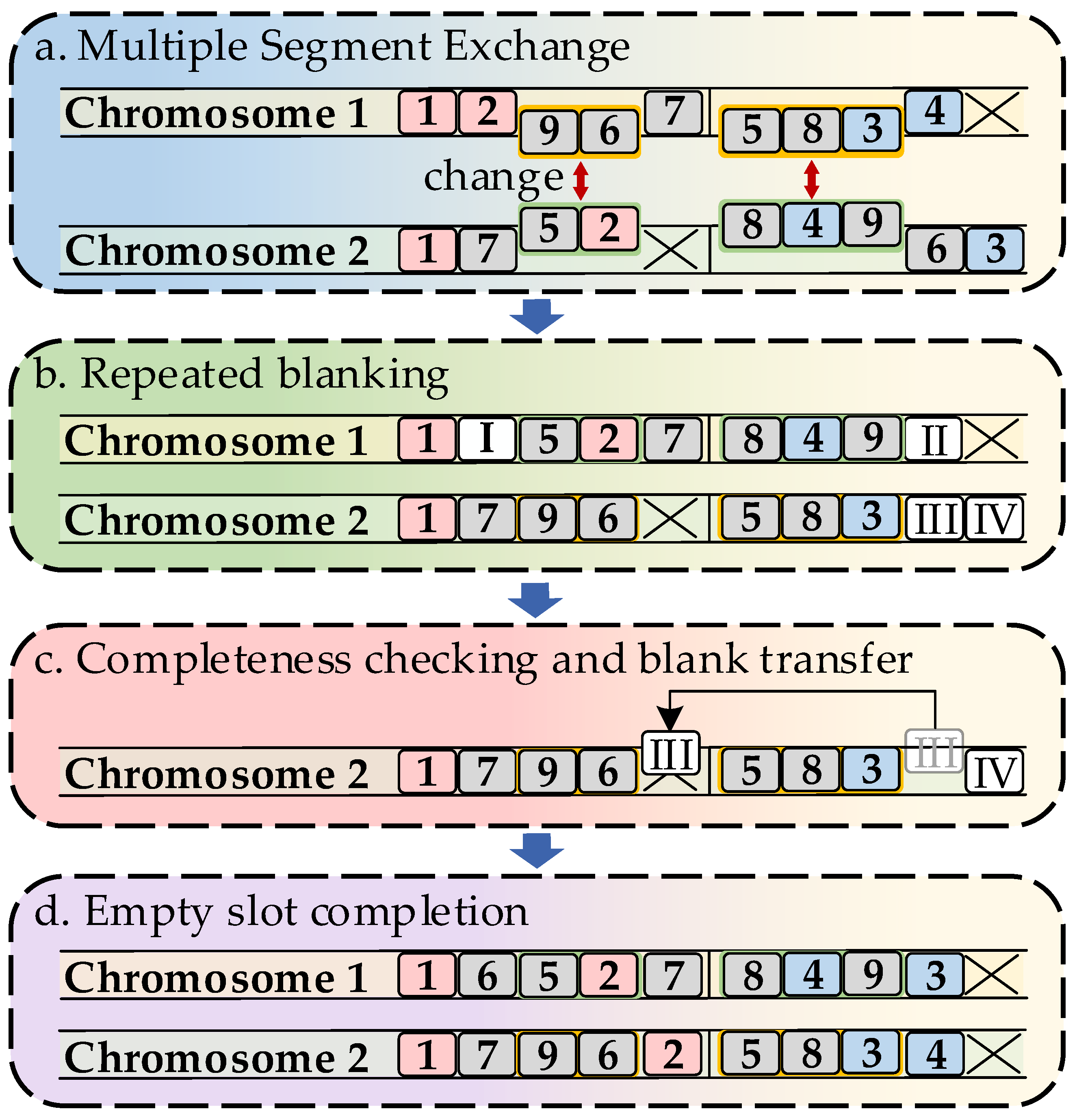
In RLSGA, the crossover is defined as follows: a chromosome randomly selects gene segments of a certain length from different positions on each path ($pat{h}_M$) and exchanges them with the corresponding gene segments of the other chromosome at the same positions and with the same length. The crossover consists of four steps: multiple segment exchange, repeated blanking, completeness checking and complementation, and blank filling. The positive segmented crossover operation on the chromosome is illustrated in Figure 6.

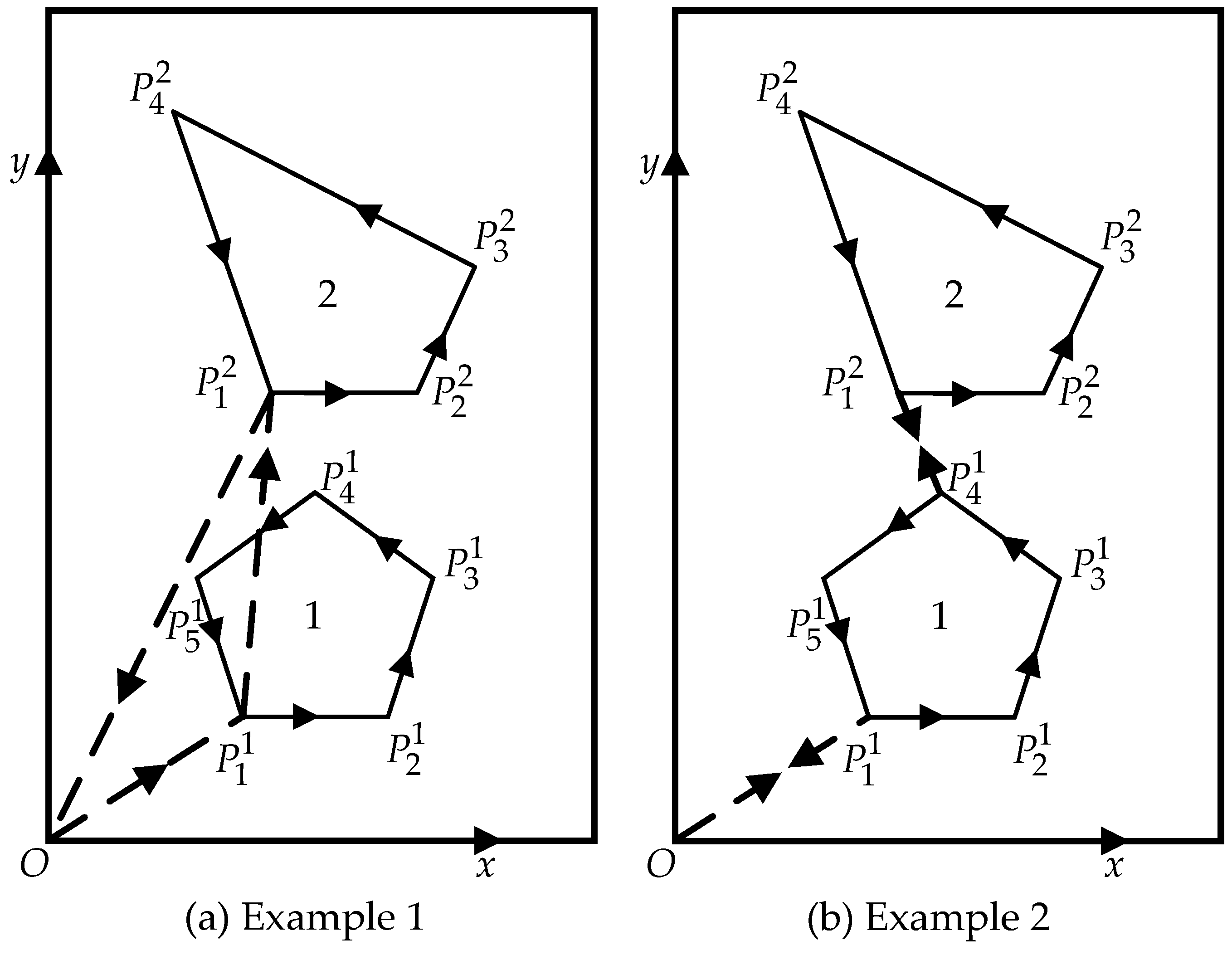
(a) Multiple segment exchange: Segmented crossover is used in RLSGA, where each chromosome comprises multiple parts of the contour line. The directions and orders of each line segment in different chromosomes are not always the same. A random section of each path is selected and exchanged to perform a forward segmented crossover operation on two chromosomes, as shown in Figure 2a. In order to ensure that the segments are of equal length and position, the start and end points for a segment are randomly selected from the shorter of the two chromosomes.

(b) Repeated blanking: After multiple segment swaps, the coding within the swapped segments remains fixed, and if there are any identical numbers outside the swapped segments, they are set to null and need to be filled. In Figure 2b, the empty positions are marked with Roman numerals on a white background. When Chromosome 1 receives the segment {5, 2} from Chromosome 2, the number 2 occurs twice outside the swapped segment, so the number outside the segment is set to null and marked as ‘I.’ Similarly, marks ‘II,’ ‘III,’ and ‘IV’ are assigned to other null positions outside the swapped segment.

(c) Completeness checking and blank transfer: Let $l_m$ be the set of part contour segments on path $m$, so $\left|l_M\right|$ is constant for path $m$. Based on this property, the completeness of the path is defined as follows: under the blank state, if the number of remaining segments on a specific path plus the number of blank spaces is less than $\left|l_M\right|$, then it is an incomplete path; if the two are equal, then it is a complete path; and if the former is greater than the latter, it is an over-complete path. Incomplete paths cannot execute the fourth step of “blank completion” because the number of their blank spaces is less than the number of segments that need to be filled. At this time, random over-complete paths are continuously transferred to the non-complete paths until they become complete. Transfer blank spaces from over-complete paths to all incomplete paths until there are no incomplete paths in the chromosome.

(d) Empty slot completion: All the segments not on the chromosome are first filled with appropriate empty slots. Then, the remaining empty slots are filled with the remaining segments in a random order according to the principle of minimal increments.

4.3.2. Reverse Segmented Crossover (RSX)

The difference between a reverse segmented crossover and a positive segmented crossover lies in the fact that, for the former, the extracted segment is reversed before being exchanged. In contrast, the latter does not reverse the extracted segment. All other steps are the same for both types of crossover.

4.3.3. Intersect Segmented Crossover (ISX)

The Intersect Segment Crossover (ISX) is designed to increase the diversity of the population. ISX only requires that the length of the segments is the same, but not their gene order. When performing ISX, after determining the segment start and end points on the shorter path, a segment of the same length is randomly selected from the long path with a satisfying starting point for the segment. Then, the two segments are exchanged. The remaining steps are the same as those for the Order Crossover.

4.4. Immediate Reward

The immediate reward feedback from the environment to the agent can reflect the rationality of its actions at the current moment in a specific state. In RLSGA, the immediate reward R of the agent is divided into three parts: the diversity reward R1, the best fitness value reward R2, and the average fitness value reward R3.

4.4.1. The Diversity Reward

In the later iterations of the GA algorithm, there is a high probability that all chromosomes in the population will converge to the same one, which quickly leads to the GA being trapped in local optima. To suppress the population assimilation rate and maintain the population’s diversity, RLSGA adds a diversity reward. The diversity reward is expressed as the change in the population diversity coefficient $div$. At time $t$, the diversity reward is calculated by the following formula:

$$R_t^1=div(po{p}_t)-div(po{p}_{t-1})$$

(7)

4.4.2. The Best Fitness Value Reward

RLSGA aims to enhance the population’s best fitness value $best[fit]$, thereby outputting it as the optimal solution for the current optimization when the iteration concludes. Therefore, positive feedback should be given to the population if the best fitness value is improved; otherwise, negative feedback will be provided. At time $t$, the reward for the best fitness value is calculated using the following formula:

$$R_t^2=\{\begin{array}{l}+1.5\hspace{0.17em}\hspace{0.17em}if\hspace{0.17em}best[fi{t}_t]>best[fi{t}_{t-1}]\\ -0.5\hspace{0.17em}\hspace{0.17em}if\hspace{0.17em}best[fi{t}_t]=best[fi{t}_{t-1}]\\ -1.0\hspace{0.17em}\hspace{0.17em}if\hspace{0.17em}best[fi{t}_t]<best[fi{t}_{t-1}]\end{array}$$

(8)

4.4.3. The Average Fitness Value Reward

The average fitness value $mean[fit]$ of a population reflects the evolutionary state and trend of the entire population. At time $t$, the reward for the average fitness value is calculated using Equation (8). It should be noted that, if the average fitness value of the population at time $t$ is equal to that at time $t-1$, it indicates that the population has likely not undergone any changes. Therefore, a substantial penalty will be imposed.

$$R_t^3=\{\begin{array}{l}+1.0\hspace{0.17em}\hspace{0.17em}if\hspace{0.17em}mean[fi{t}_t]>best[fi{t}_{t-1}]\\ -2.0\hspace{0.17em}\hspace{0.17em}if\hspace{0.17em}mean[fi{t}_t]=best[fi{t}_{t-1}]\\ -0.5\hspace{0.17em}\hspace{0.17em}if\hspace{0.17em}mean[fi{t}_t]<best[fi{t}_{t-1}]\end{array}$$

(9)

The immediate reward of an agent at time $t$ is the sum of three components:

$$R_t=R_t^1+R_t^2+R_t^3$$

(10)

4.5. RLSGA Learning and Iterative Process

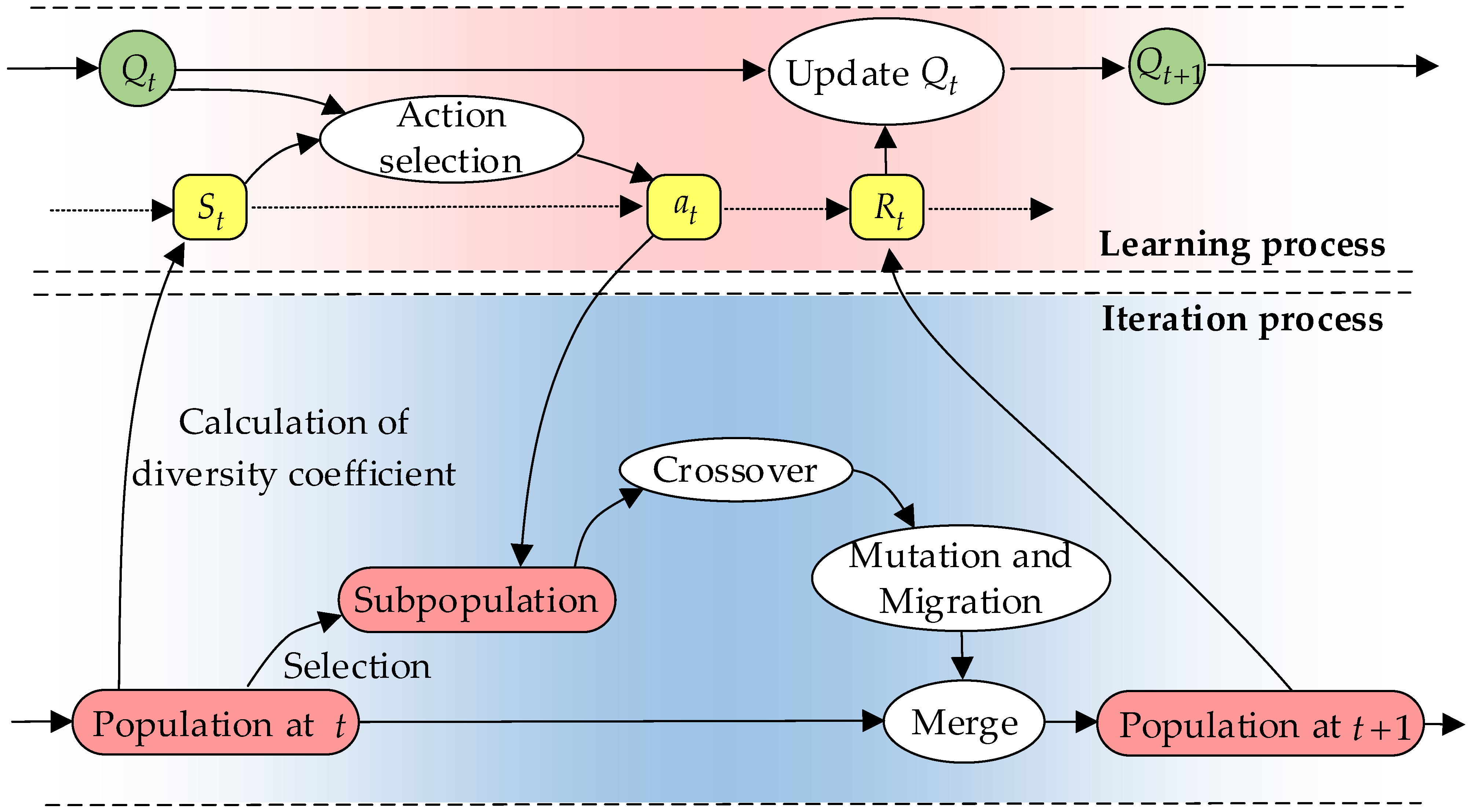
In summary, the learning and iteration process of the agent in RLSGA is illustrated in Figure 7.

In Figure 7, $Q_t$ is the $Q$ table at time $t$, which is used to store the accumulated rewards of different actions in each state. The $Q_t$ table is updated using the $Q-learning$ algorithm, where the action sampled in a single step is independent of the action selected at time $t$. The $Q_t$ table is updated based on Equation (11) in the $Q-learning$ algorithm, with $\alpha \in [0,\hspace{0.17em}1)$ representing the learning rate and $\gamma \in [0,\hspace{0.17em}1]$ representing the discount factor. The $Q-learning$ algorithm allows the agent to learn incrementally and update the accumulated rewards during the iteration process. As a result, the agent can more accurately determine what actions to take in the current state to maximize its return as the iteration progresses.

$$Q_{t+1}(s_t,\hspace{0.17em}{a}_t)=(1-\alpha )Q_t(s_t,\hspace{0.17em}{a}_t)+\alpha [R_t+\gamma Q_t(s_{t+1},\hspace{0.17em}{a}_{t+1})]$$

(11)

The basic process of the RLSGA algorithm can be summarized as follows:

• Selection: Use roulette wheel selection to choose $n$ individuals from a population of size $Q-learning$ to form a subpopulation.
• Action selection: The population obtains the state $s_t$ based on its diversity coefficient and then selects an action (crossover operator) based on the state and the cumulative reward $Q_t$. The action selection method uses an $\epsilon$-greedy approach, where an action is randomly selected with probability $\epsilon \hspace{0.17em}(\epsilon \in [0,\hspace{0.17em}1])$, and the action with the maximum cumulative reward is selected with probability $1-\epsilon$.
• Crossover: The individuals in the subpopulation undergo crossover with a probability of $pC$.
• Mutation: Each individual in the subpopulation undergoes a mutation with a probability of $pMu$, which is defined as the exchange of two random encodings on a random path.
• Migration: Each individual in the subpopulation undergoes migration with a probability of $pMi$, where migration is defined as transferring a random segment of a random path to a random position on another path.
• Merge population: The subpopulation and parent population consist of $2n$ individuals. After merging the two populations, the top $n$ individuals with high fitness values are selected as the next-generation population.
• Obtain immediate reward: Obtain the immediate reward $R_t$ based on the relationship between the fitness values and diversity coefficient of the current and previous generations.
• Update $Q_t$ to $Q_{t+1}$.$P_1^1$

5. Experimental Results and Discussions

For the proposed HPCPO model, two test questions are designed in this paper. On the test problem, the effectiveness of RLSGA is checked.

The methods have been implemented using the Python programming language, and the experimental environment has been a computer with Windows 10, an Intel(R) Core(TM) i7-10875H CPU @ 2.30 GHz, and 16.0 GB RAM (Lenovo, located in Shanghai, China).

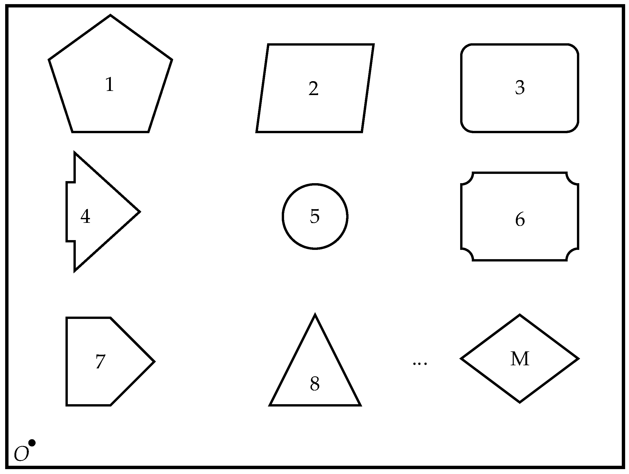
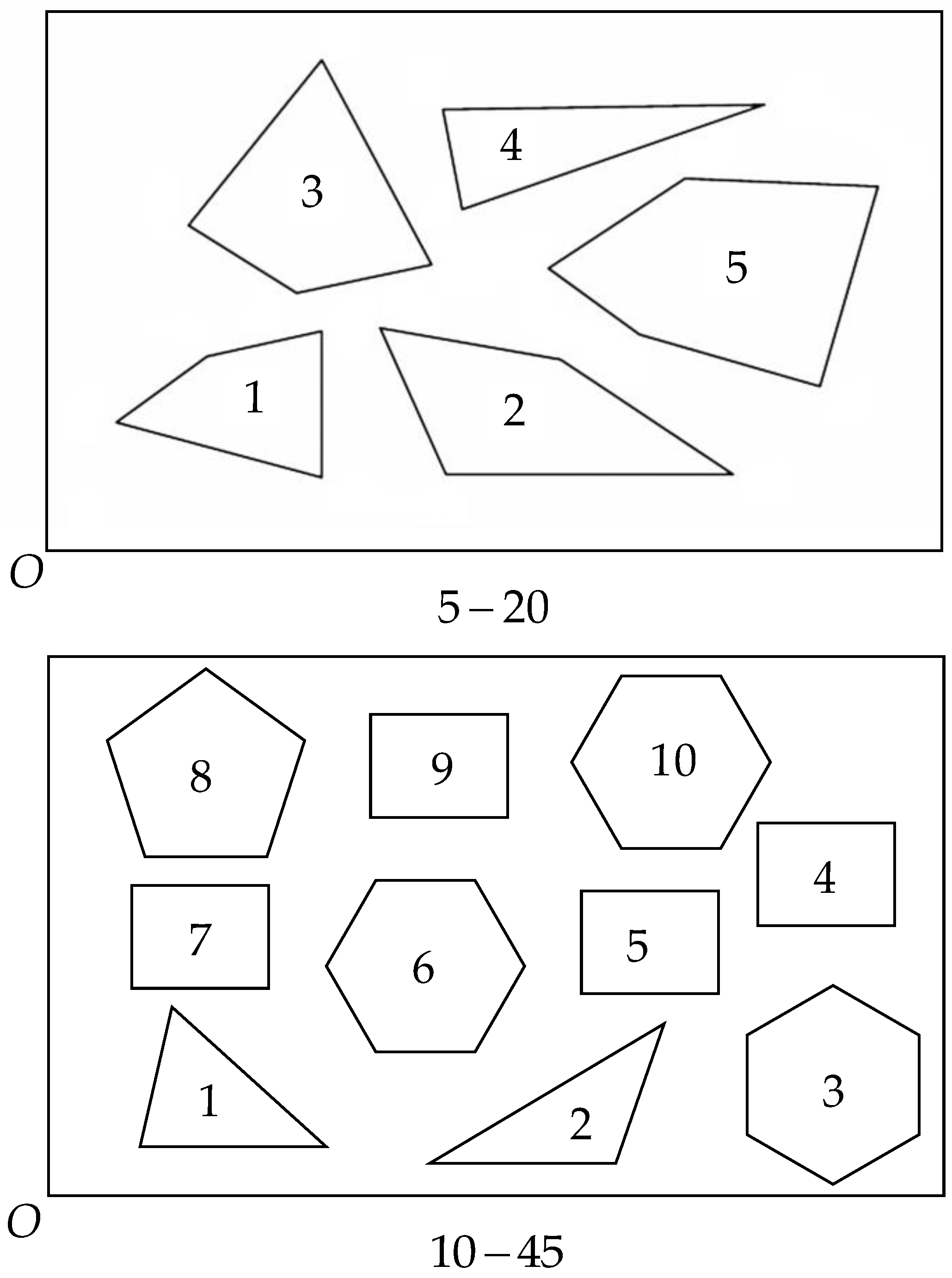
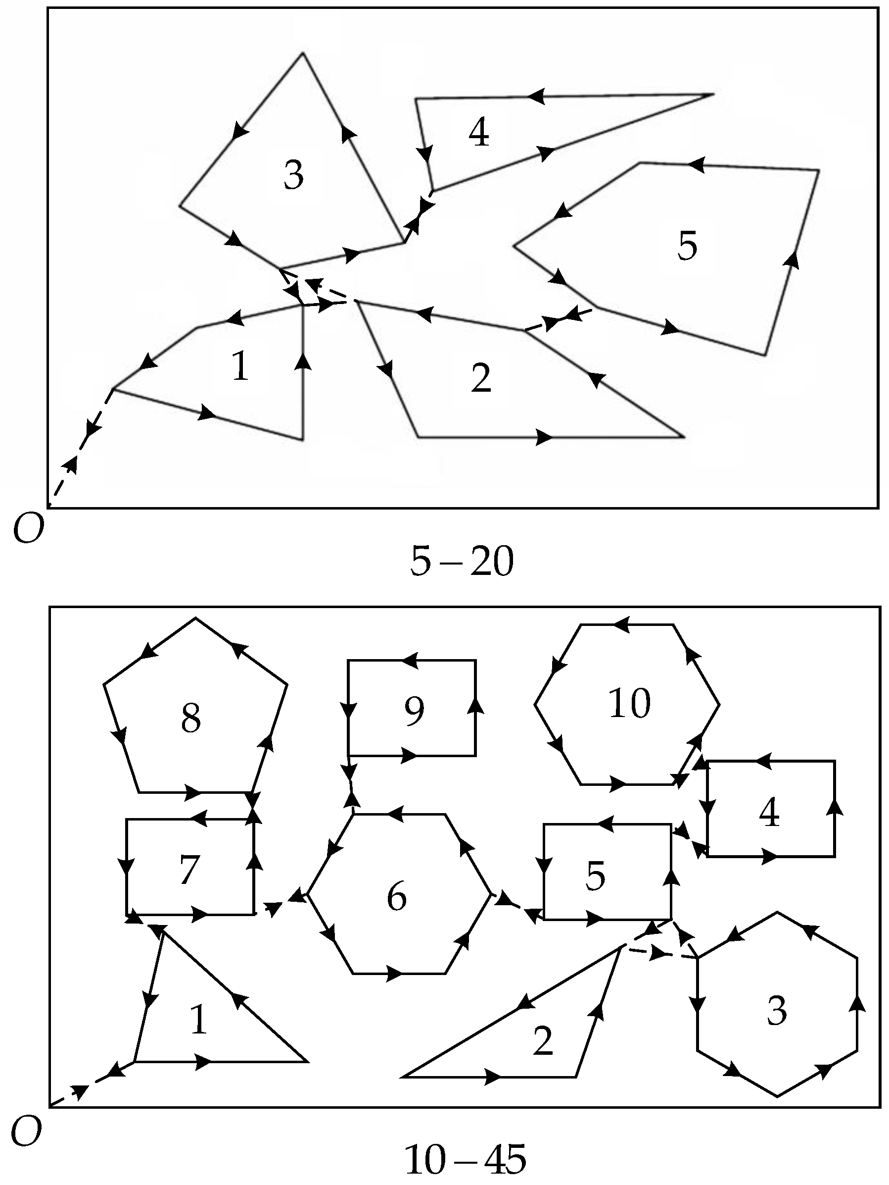
5.1. Test Question Design

In this paper, a total of two test questions of two scales are designed, including five parts with 20 line segments (5–20) and ten parts with 45 line segments (10–45). The layout of the two test questions is shown in Figure 8.

5.2. Comparing Algorithms and Algorithm Parameters

The particle swarm optimization (PSO) algorithm [29], the optimal foraging algorithm (OFA) [30], and the whale optimization algorithm (WOA) [31] are excellent heuristic algorithms. In this paper, the above three heuristic algorithms are selected as the comparison algorithms for RLSGA. Specifically, to verify the impact of the reinforcement learning framework on genetic algorithms (GA), we included a segmented genetic algorithm (SGA) without a reinforcement learning framework in the comparison algorithms. This algorithm does not have attributes such as a population state or immediate rewards and randomly selects a crossover operator during chromosome crossover.

The algorithm parameters were set as follows. For PSO, we set the inertia weight $\omega$ to 0.3 and the acceleration coefficients $c_1$ and $c_2$ to 0.5, which are commonly used values in the literature [29]. For OFA, we set the parameter k to $0.9-0.5\frac{t}{t_{\max }}$. This parameter setting enables OFA to dynamically adjust the exploration–exploitation tradeoff during the optimization process [30]. Regarding WOA, we used the default parameter values mentioned in [31], which were suitable for our problem domain. Specifically, we set $A$ = 2, $A_{\min }$ = 0, $C$ = 1, and $b$ = 1, as recommended in [31]. It is worth noting that the parameters of the segmented genetic algorithm (SGA) without a reinforcement learning framework were set the same as those of the reinforced learning segmented genetic algorithm (RLSGA) during the iterative process. Since the parameter-tuning process in the reinforcement learning phase is a time-consuming task, the hyperparameter settings adopted in this study are based on existing research (Alipour et al.) and further tuned [32]. Specifically, we set $pC$ = 0.6, $pMu$ = 0.1, and $pMi$ = 0.1 during the iterative process, and $\alpha$ = 0.9, $\gamma$ = 0.9, and $\epsilon$ = 0.1 during the learning process.

The five algorithms used the same randomly initialized population as the initial population for optimization. The population size n for the five algorithms on test problems 5–20 and 10–45 were all set to 100 and 200, and the maximum iteration times were set to tmax = 1000. Each algorithm was independently run 30 times on each test problem.

5.3. Experiment and Analysis

Table 3. Algorithm-running results comparison.

Case	Average Total Path Lengths					Best Total Path Lengths
	RLSGA	PSO	OFA	WOA	SGA	RLSGA	PSO	OFA	WOA	SGA
5–20	49.68	56.36	54.95	53.96	53.34	49.68	55.95	54.38	53.14	52.09
10–45	84.31	97.65	97.19	102.30	95.49	81.79	96.17	92.51	98.78	92.32

presents the average and best (indicated in bold) total path lengths obtained by the five algorithms, each independently run 30 times on the test problems. RLSGA achieved the best performance on the average and best values for each test problem. The gap between the average and best values obtained by RLSGA was significantly smaller than that of the other algorithms, indicating that RLSGA had lower randomness and more stable performance. For the more straightforward problem 5–20, all algorithms successfully obtained the optimal solution in every run. As the number of parts or part profiles in the test problem increased, the complexity of the problem also increased. RLSGA significantly outperformed the other algorithms on the 10–45 test problem. Overall, RLSGA had the best performance, followed by SGA and PSO, while OFA and WOA did not perform as well. The results indicate that RLSGA can effectively and reasonably optimize the HPCPO model.

Figure 9 is the tool path corresponding to the optimal solution of RLSGA on the two test problems.

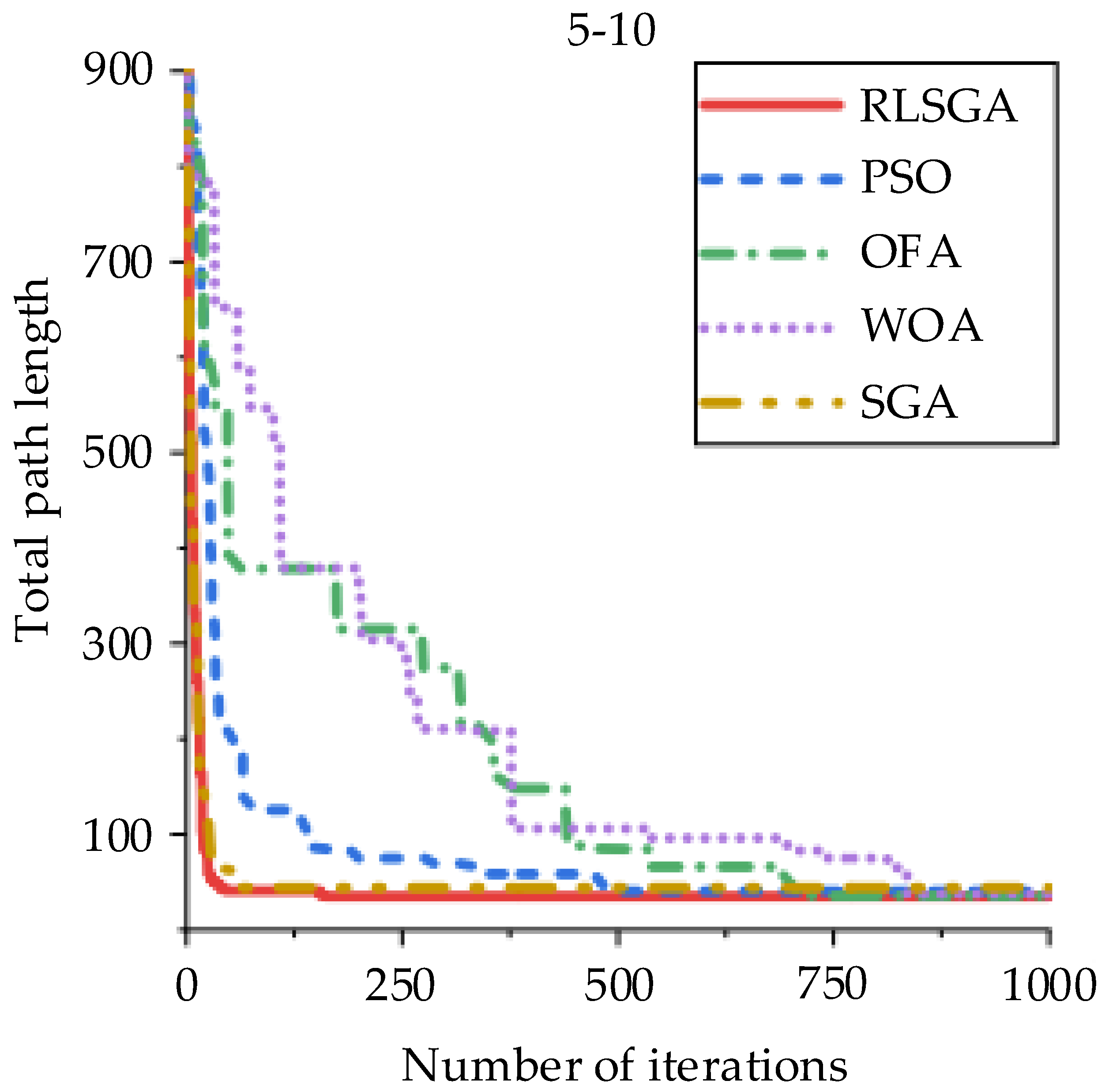
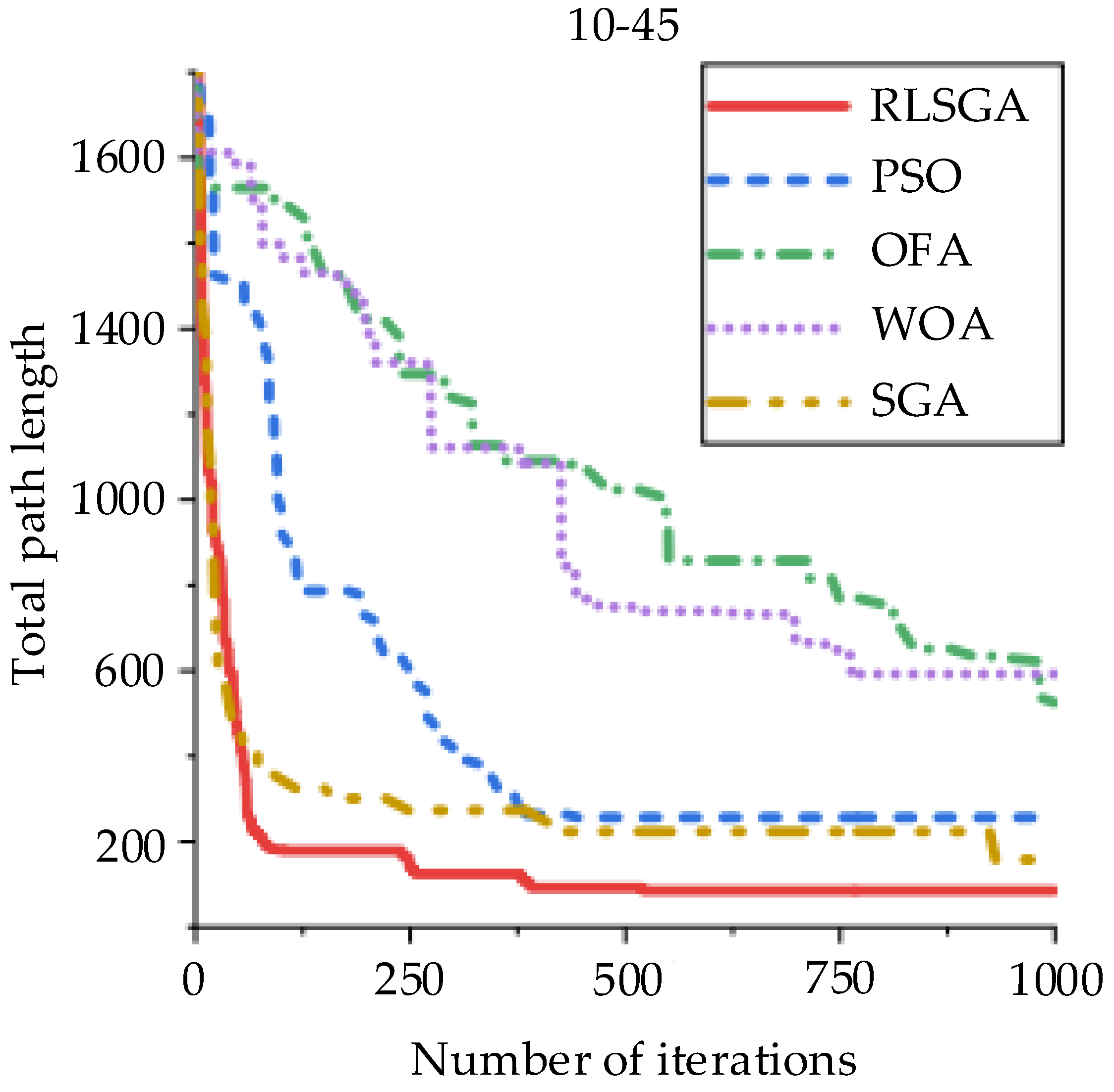
The convergence behavior of the five algorithms on the 5–20 and 10–45 test problems is shown in Figure 10 and Figure 11, respectively. In general, all algorithms demonstrate a gradual convergence to the optimal solution, although there are variations in the convergence rate and the quality of the final solution.

On the 5–20 problem, RLSGA, SGA, and PSO show a relatively fast convergence, while OFA and WOA converge more slowly, as shown in Figure 10. Specifically, RLSGA and SGA converge almost simultaneously after 100 iterations, suggesting that both methods effectively explore the search space and exploit reasonable solutions. By contrast, the convergence curve of OFA exhibits more fluctuations, indicating that the algorithm may have difficulty escaping from local optima. Meanwhile, WOA converges steadily but more slowly than the other methods, indicating that its exploration strategy may need to be more effective in this problem.

On the 10–45 problem, RLSGA outperforms the other methods by a large margin, as shown in Figure 11. RLSGA and PSO converge to the optimal solution after about 1000 iterations, while SGA falls into a local optimum and only finds a better solution at the end of the iteration. This result suggests that the diversity reward in RLSGA effectively prevents premature convergence and maintains population diversity, enabling the algorithm to explore more promising regions of the search space.

To better understand the performance of the five algorithms, we compared their computational cost in terms of time complexity. Precisely, we measured the average running time of each algorithm on the 5–20 and 10–45 test problems. The results are presented in

Table 4. Comparison of average running times of five algorithms on test problems 5–20 and 10–45.

Algorithm	Test Problem 5–20	Test Problem 10–45
RLSGA	16.523	27.714
SGA	16.003	26.660
PSO	24.671	46.529
OFA	30.587	50.319
WOA	35.641	55.413

The data in the table are in seconds.

. As shown in Table 4, RLSGA and SGA have the lowest average running times on both test problems, while PSO, OFA, and WOA have higher running times. Although RLSGA’s running time is slightly higher than SGA’s, the difference is within an acceptable range, considering RLSGA’s better performance in finding optimal solutions. These results indicate that RLSGA and SGA are the most computationally efficient algorithms for solving the HPCPO problem among the five compared algorithms. Specifically, RLSGA outperforms the other algorithms, including SGA, regarding solution quality and convergence speed.

We can draw several conclusions based on the performance of RLSGA, SGA, and other comparison methods on the 5–20 and 10–45 problems. Firstly, RLSGA outperforms all other comparison methods, suggesting that the reinforcement learning framework with diversity reward effectively solves the HPCPO problem. Secondly, SGA performs better than OFA and WOA but outperforms RLSGA and PSO. This indicates that the genetic algorithm is a suitable method for this problem but may require additional improvements in the future.

To better understand the reasons for the superior performance of RLSGA, we further analyzed its behavior during the optimization process. Specifically, we observed that RLSGA sacrifices some convergence speed to maintain diversity. However, this tradeoff leads to a more robust and stable algorithm less likely to be trapped in local optima. The convergence curves of RLSGA on both problems are relatively smooth, indicating that the algorithm can consistently find reasonable solutions. This property is significant for real-world applications where the objective function may be noisy or non-differentiable.

Furthermore, we compared the results of RLSGA with those of SGA and found that RLSGA is superior in terms of convergence rate and solution quality. The success of RLSGA is due to the use of a reinforcement learning framework, which allows the algorithm to learn from past experiences and adapt to changes in the optimization landscape. Additionally, the diversity reward function in RLSGA encourages the algorithm to explore a wide range of solutions, which may help to avoid getting stuck in local optima.

In conclusion, our results demonstrate the effectiveness of the RLSGA algorithm for solving the HPCPO problem. The use of a reinforcement learning framework and a diversity reward function are key factors contributing to the superior performance of RLSGA. Further research can explore how to further improve the performance of genetic algorithms on this problem by incorporating additional techniques or optimizing the algorithm’s parameters.

6. Conclusions

This paper proposes a hull parts cutting path optimization problem (HPCPO) model based on partial cutting rules for the laser cutting process of ship components in practical production activities. The HPCPO model represents the optimization of cutting paths for each component as the planning of the cutting sequence of each component’s contour segments. To optimize the HPCPO, this paper proposes a reinforcement -learning-based segmented genetic algorithm (RLSGA), which enables the population to try and accumulate different segmented crossover operators at different diversity coefficient states to achieve maximum benefits. The performance of RLSGA is compared with four other algorithms on the designed test problem, and the results show that RLSGA outperforms the other algorithms and effectively solves the HPCPO problem.

The results show that the proposed reinforcement-learning-based segmented genetic algorithm (RLSGA) performs better than other algorithms in solving hull parts cutting path optimization problems based on partial cutting rules (HPCPO). However, there are still several directions for future work. Firstly, additional factors relevant to practical production activities, such as machine maintenance, should be considered to enhance the HPCPO model. Secondly, a more comprehensive comparison with other state-of-the-art algorithms in the field should be conducted to validate the RLSGA algorithm’s effectiveness further. Lastly, it may be worthwhile to investigate the applicability of the RLSGA algorithm to other optimization problems in the field of laser cutting and other manufacturing domains.