An Algorithm of Complete Coverage Path Planning for Unmanned Surface Vehicle Based on Reinforcement Learning

Abstract

A deep reinforcement learning method to achieve complete coverage path planning for an unmanned surface vehicle (USV) is proposed. This paper firstly models the USV and the workspace required for complete coverage. Then, for the full-coverage path planning task, this paper proposes a preprocessing method for raster maps, which can effectively delete the blank areas that are impossible to cover in the raster map. In this paper, the state matrix corresponding to the preprocessed raster map is used as the input of the deep neural network. The deep Q network (DQN) is used to train the complete coverage path planning strategy of the agent. The improvement of the selection of random actions during training is first proposed. Considering the task of complete coverage path planning, this paper replaces random actions with a set of actions toward the nearest uncovered grid. To solve the problem of the slow convergence speed of the deep reinforcement learning network in full-coverage path planning, this paper proposes an improved method of deep reinforcement learning, which superimposes the final output layer with a dangerous actions matrix to reduce the risk of selection of dangerous actions of USVs during the learning process. Finally, the designed method validates via simulation examples.

1. Introduction

In recent years, the field of USV based on sensor technology and intelligent algorithms has made great progress [1]. During the working process, USV first uses sensors to model the working environment, estimates its own state, and then makes decisions based on the surrounding environment and its own state to complete the corresponding tasks. Compared with humans, USVs are more suitable for performing some highly dangerous or repetitive tasks, such as target reconnaissance [2], hydrographic mapping [3], and water patrol [4]. To accomplish these tasks in unpredictable water environments, path planning techniques are crucial for USVs.

As an important aspect of robotics, coverage path planning (CPP), is special path planning. full-coverage path planning requires that the generated USV motion trajectory can cover all areas in the workspace, except obstacles, to the greatest extent. The full-coverage path planning algorithm has a wide range of applications, such as unmanned surface vehicles [5,6,7], intelligent sweeping robots [8], gardening electric tractors [9], cleaning robots [10,11], tile robots [12], rescue robots [13], window cleaning robot [14], automatic lawn mower [15], etc. In practice, there are many optimization algorithms that USV can use, such as the Taguchi method, ant colony algorithm, fuzzy logic, and TLBO, which provide many options for the design of path planning. The Taguchi method is an analytical approach for a design algorithm, first proposed to enhance the quality of products in manufacturing. Wang et al. [16] designed optimal bridge-type compliant mechanism flexure hinges with low stress by using a flexure joint. Sun et al. [17] proposed a new binary fully convolutional neural network (B-FCN) based on Taguchi method sub-optimization for the segmentation of robotic floor regions, which can precisely distinguish floor regions in complex indoor environments. The ant colony optimization algorithm is a bionic intelligent algorithm inspired by the foraging behavior of ant colonies. A global path planning algorithm based on an improved quantum ant colony algorithm (IQACA) is proposed by Xia et al. [18]. Fuzzy logic has gained much attention due to its ease of implementation and simplicity. The concept behind it is to smooth the classical Boolean logic of true (1 or yes) and false (0 or no) to a partial value located between these values, coming in a term of the degree of membership. Abdullah Alomari et al. [19] proposed a novel, distributed, range-free movement mechanism for mobility-assisted localization based on fuzzy-logic approach. Teaching a learning-based optimization (TLBO) algorithm is a distinguished, nature-inspired, population-based meta-heuristic, which is basically designed for unconstrained optimization. Wang et al. [20] proposed a novel approach to improve centrifugal pump performance based on TLBO.

In recent years, due to the new demand for USVs with full-coverage path planning in various fields, such as civil, military, patrol [21], search and rescue [22,23,24,25], cybersecurity industry [26], and inspection [27,28], scholars and experts from various countries have proposed various methods to complete the task of full-coverage path planning.

The full-coverage path planning algorithm based on the intelligent algorithm means that USV first models the environment through sensors and relies on the modeled map to perform full-coverage path planning [29]. The grid map is a common expression of the environment, and it divides the map into several square grids, which can be used for a full-coverage route plan. The full-coverage path planning algorithm, based on the traditional algorithm, includes the full-coverage path planning algorithm of boustrophedon or the inner spiral full-coverage path planning [30,31]. The boustrophedon method drives the USV to go back-and-forth along a path, similar to that of an ox plowing a field. In the work area that needs to be covered, the USV performs full-coverage path planning work with certain direction rules. Once an obstacle is encountered, the USV changes direction to cover in another direction. Lee et al. [32] proposed a full-coverage path planning algorithm based on the inner spiral. This algorithm is an online full-coverage path planning algorithm, which ensures complete coverage in unstructured planar environments. However, this kind of algorithm does not introduce global control [33], and the USV can only perceive the regional state within a certain range, instead of global information, so it will lead to a large cumulative error.

The most classic full-coverage path planning algorithm based on the exact cell decomposition method was proposed by Choset [34] in 2000. Choset developed an accurate cell decomposition method for full-coverage path planning, which is essentially a generalization of trapezoidal decomposition. It can be used in work environments with non-polygonal obstacles and is more efficient than trapezoidal decomposition. Zhu et al. [35] proposed the Glasius bionic neural network (GBNN) algorithm and improved this algorithm in view of the shortcomings of the bionic neural network algorithm, such as high computational complexity and long path planning time. This algorithm constructs a grid graph by discretizing the two-dimensional underwater environment and then establishes a corresponding dynamic neural network on the grid graph. Luo et al. [36] first proposed a complete coverage neural network (CCNN) algorithm for ultrasonic motor path planning. By simplifying the calculation process of neural activities, this algorithm can significantly reduce the calculation time. In order to improve coverage efficiency and generate more standardized paths, the author establishes the optimal next-step location decision formula, combined with the coverage direction term.

However, the above studies mainly focus on the coverage rate, and a systematic study on the coverage path repetition rate is rare. In this study, a new full-coverage path planning algorithm based on reinforcement learning is proposed. In the decision phase, USV can use the model learning capability of reinforcement learning to select actions based on the historical information of the area coverage. In the training phase, the information of area coverage is used to train the neural network, which makes the neural network model fit the best motion action. This algorithm improves the defects of the traditional full-coverage path planning algorithm with higher efficiency. Both ensure the coverage rate and significantly reduce the coverage path repetition rate. The feasibility and efficiency of the algorithm are verified in simulation experiments. This contribution is expected to provide a scientific reference for the future research about the coverage path repetition rate.

2. USV Models and Environment Modeling

2.1. USV Model

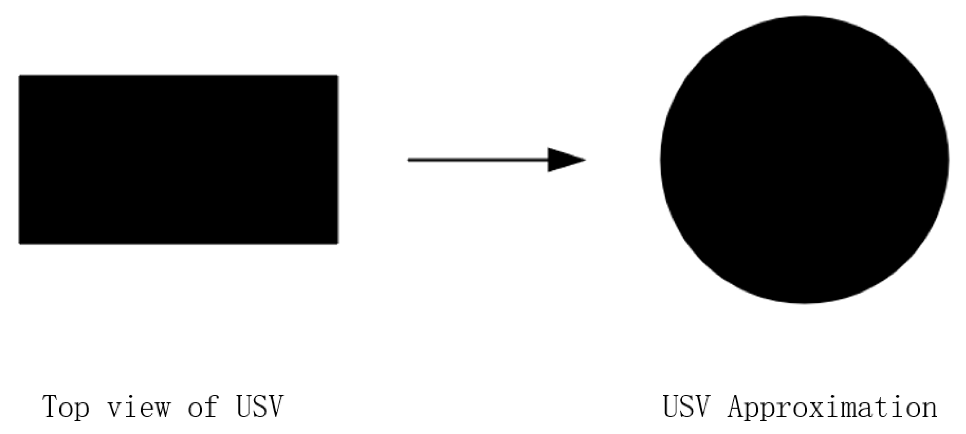
When the USV moves in the workspace, in order to avoid the USV colliding with the obstacles or the map boundary, it is necessary to model according to the size and shape of the USV. In path planning, there are two ways to model the USV. The first one is to model the USV in real-time and the second one is to inflate obstacles to a width the size of the vehicle’s radius. Since the first method needs to model the USV in real-time, it can move the USV irregularly with a better effect and stronger robustness, but it consumes too many computing resources and is difficult to implement. The obstacle avoidance effect is very good, but the efficiency of the path planning is too low. 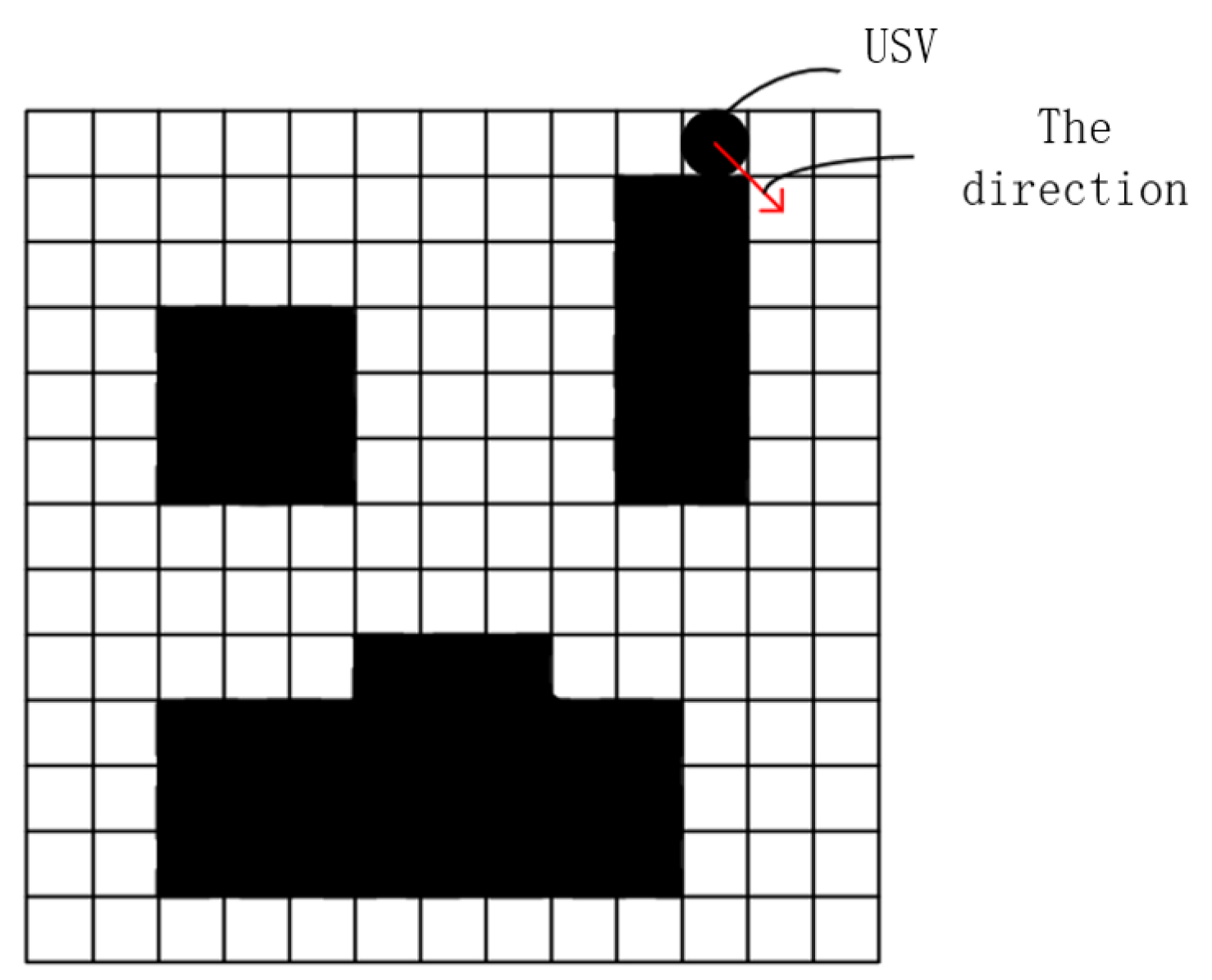In the second method, an irregular USV can be regarded as a circular USV with a diameter equal to the maximum width of the USV, as shown in Figure 1. The model diagram of the USV is a subset of the approximate model of the USV, that is, the area of the approximate model of the USV is greater than or equal to the model diagram of the USV, so as long as the approximate model of the USV does not collide with obstacles, the USV can be guaranteed. During the movement, it is possible not to collide with obstacles. This will not lose too much USV modeling accuracy, but also has the advantages of good real-time performance, convenience, reliability, and high efficiency. Since the grid size selected in this paper is equal to the diameter of the approximate image of the USV, the target point moved by the USV each time can be set as the midpoint of the next grid, and when the USV needs to move obliquely, it is very likely that, as shown in Figure 2, in order to simplify the kinematic model of the USV, this paper sets the movement direction of the USV to only the horizontal and vertical directions and does not support the oblique direction. The red arrows in Figure 2 indicate the direction of usv’s oblique motion.

2.2. Workspace Modeling and Preprocessing

When the USV uses the grid map modeling method for full-coverage path planning, the resolution of the grid map has a great influence on the efficiency of its algorithm. If the resolution is too high, the map information will be redundant, will take up a lot of memory, and will even lead to repeated traversal, which will reduce the efficiency of the full-coverage path planning algorithm. When the resolution is too low, although the memory footprint of the grid map will become very small, it cannot represent some details of the environmental map, and there is a high probability that the blank area around the obstacle will be represented as the obstacle area, so using low-resolution raster maps results in lower coverage for USVs. Therefore, when modeling the working environment of the USV, in order to reduce the memory occupied by the map and represent some details of the environment, this paper adopts the coverage size of the USV as the resolution size, that is, the size of each grid is the size that the USV can use once. The size of the coverage area. When the USV reaches the middle position of the grid, it is considered that the grid has been covered by the USV.

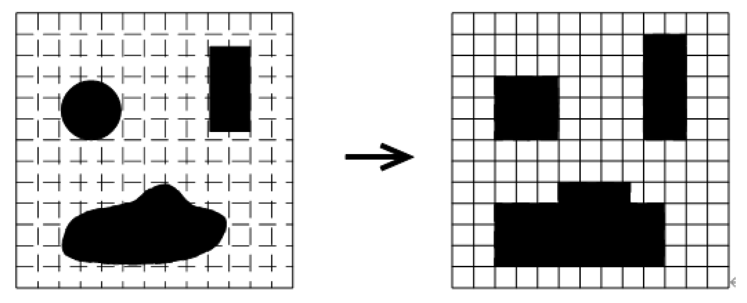
The construction method of the grid map in this paper is to first divide the working environment of the USV into several grids of the same size, set the grid that the USV can reach and cover as white with a value of 0, and set the grid where the obstacles are located. The grid is set to black, with a value of −1. However, there is only a part of obstacles in some grids, that is, there are both white areas and black areas in this grid. Here, in order to prevent the USV from being damaged by collisions when performing full-coverage tasks, this paper uses such grids. Unpassable areas are uniformly set to black. The construction method of the grid map is shown in Figure 3.

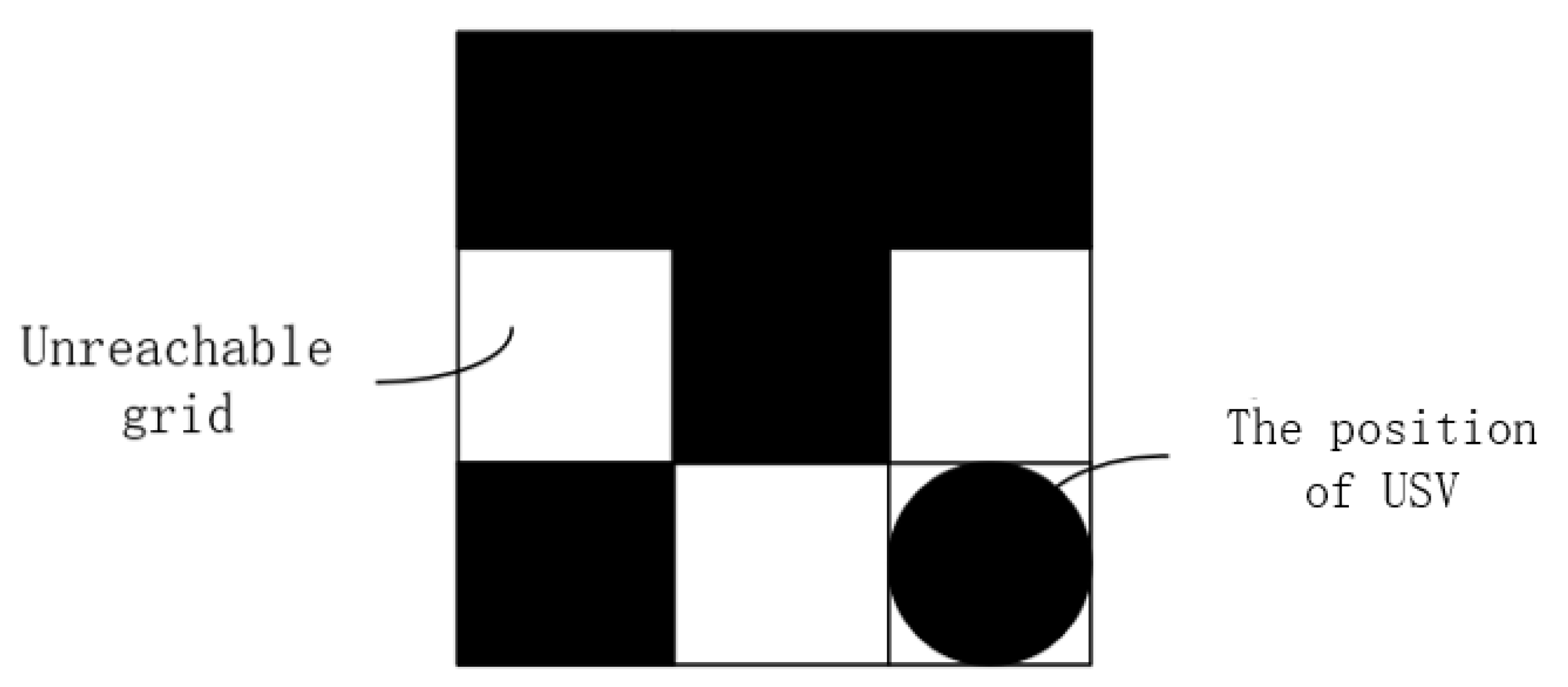
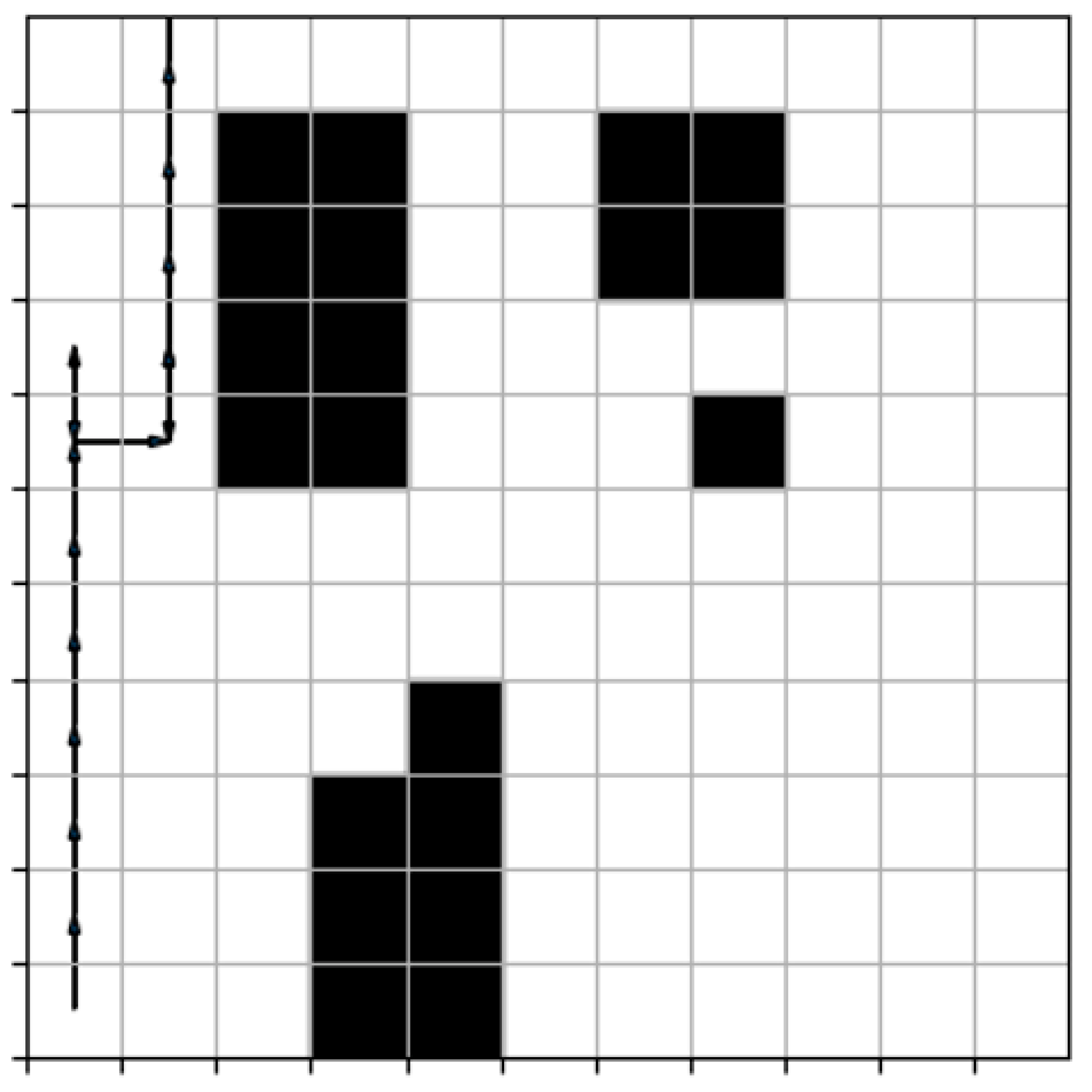
In order to realize the full-coverage path planning of the USV, it is first necessary to determine the area that the USV needs to cover. In the grid map, the general area that the USV needs to cover is all the blank grids in the grid map, but there are some special For example, if an obstacle surrounds a blank grid, although there is no obstacle in the surrounded grid, the USV cannot pass through the obstacle to cover the grid, as shown in Figure 4. Therefore, it is necessary to deal with this situation, that is, the non-coverable grid becomes the grid with obstacles.

The difficulty of this task lies in how to use the algorithm to automatically find the non-coverable grids. The non-coverable grids can be easily found by human judgment, but for the computer, the map is just a series of two-dimensional matrices inputs. For this reason, this paper proposes a raster map preprocessing method to remove non-overridable rasters.

Since the memory occupied by the matrix is much smaller than the memory occupied by the image, and each element in the matrix of the same dimension as the grid map can corresponds to the grid in the grid map, the grid map preprocessing method is proposed in this paper. First, the grid map is converted into a two-dimensional state matrix form. The element value of the blank grid in the corresponding position in the state matrix is 0, and the element value of the black grid representing the obstacle in the corresponding position in the state matrix is −1. The element value of the corresponding position of the covered grid in the state matrix is 1, and the element value of the corresponding position of the grid where the USV is located in the state matrix is 7. In the preprocessing stage of the grid map, the location of the USV does not need to be considered, and the USV cannot appear in the grid where obstacles exist, so the element value corresponding to the grid where the USV is located is recorded as 0 in the preprocessing stage. The grid map shown in Figure 4 is converted into a two-dimensional matrix, as shown in matrix 1.

$$\left[\begin{array}{ccc}-1& -1& -1\\ 0& -1& 0\\ -1& 0& 0\end{array}\right]$$

(1)

Because the surrounding of the map is the map boundary, the map boundary is regarded as an obstacle, and the USV should not go out of the map boundary, so firstly, add −1 around the two-dimensional matrix representing the grid map, as shown in matrix 2.

$$\left[\begin{array}{ccccc}-1& -1& -1& -1& -1\\ -1& -1& -1& -1& -1\\ -1& 0& -1& 0& -1\\ -1& -1& 0& 0& -1\\ -1& -1& -1& -1& -1\end{array}\right]$$

(2)

Then, set a 3 × 3 matrix and denote it as a screening matrix $M_f$, which is matrix 3.

$$\left[\begin{array}{ccc}0& 1& 0\\ 1& 4& 1\\ 0& 1& 0\end{array}\right]$$

(3)

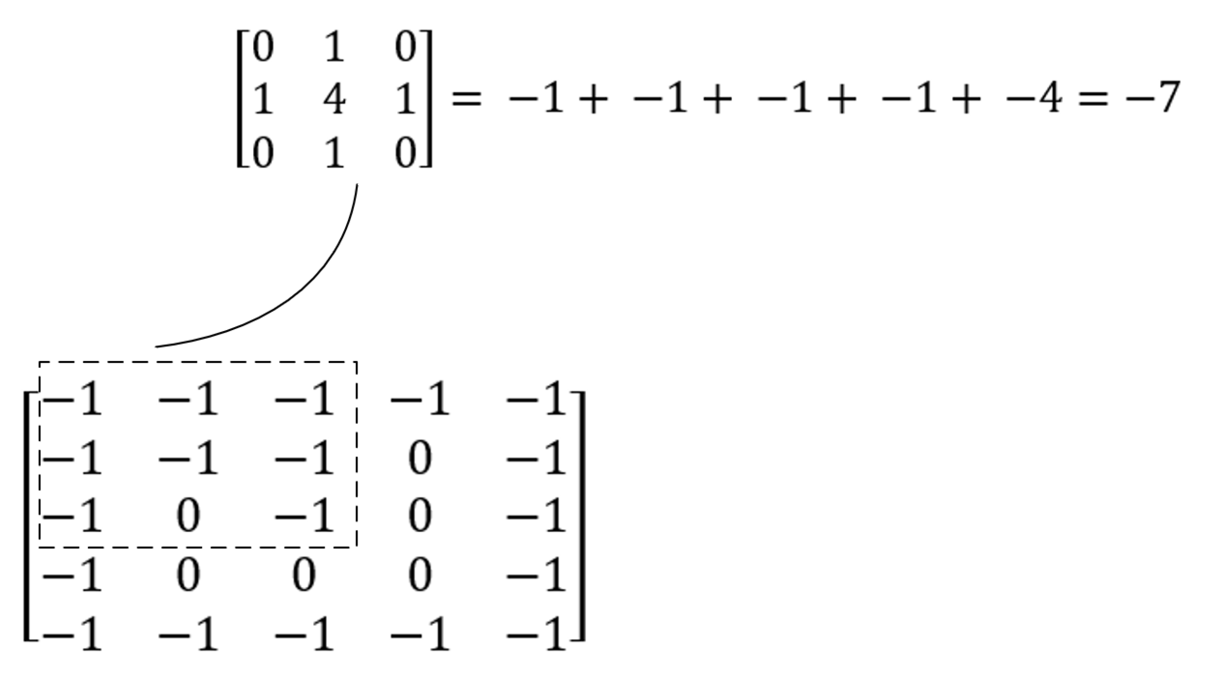
Decompose matrix 2 into (n−2) × (n−2) 3 × 3 matrices, where n is the dimension of the matrix after adding −1, and then do a dot product operation with matrix 3. That is, multiply and sum the elements of each position of the two 3 × 3 matrices, and finally, obtain a 3 × 3 matrix, and write the obtained result into a matrix of the same size as matrix 1. The calculation process is shown in Figure 5. The final result is matrix 4.

$$\left[\begin{array}{ccc}-7& -7& -3\\ -4& -5& -2\\ -6& -3& -2\end{array}\right]$$

(4)

Then, filter the generated matrix. If the value of a certain position is less than or equal to −4, the grid representing the position is an uncoverable point or an obstacle, and the value corresponding to the element of its position should be −1. The other grids are grids that need to be fully covered, and the element value corresponding to their position is 0. The two-dimensional matrix corresponding to the filtered raster map is shown in matrix 5. Use this method to correctly and efficiently remove non-overridable blank rasters, turning them into black rasters.

$$\left[\begin{array}{ccc}-1& -1& -1\\ -1& -1& 0\\ -1& 0& 0\end{array}\right]$$

(5)

In the process of performing the full-coverage task, use this matrix to record the grid where the USV is located and the grid that the USV has covered. The element value of the corresponding matrix position is changed from 0 to 1, and the element value of the matrix position corresponding to the rest of the grids remains unchanged. The matrix corresponding to Figure 6 is shown in matrix 6.

$$\left[\begin{array}{ccccccccccc}0& 0& 0& 0& 0& 0& -1& -1& -1& -1& -1\\ 0& 0& 0& 0& 0& 0& 0& 0& 0& 0& 0\\ 0& 0& -1& -1& -1& -1& 0& 0& 0& 0& 0\\ 0& 0& -1& -1& -1& -1& 0& 0& 0& 0& 0\\ 0& 0& -1& -1& -1& -1& 0& 0& -1& 0& 0\\ 0& 0& -1& -1& -1& -1& 0& 0& -1& 0& 0\\ 0& 0& 0& 0& 0& 0& 0& 0& -1& 0& 0\\ 1& 1& 1& 1& 7& 0& 0& 0& -1& 0& 0\\ 1& 0& 0& 0& 0& 0& 0& 0& -1& 0& 0\\ 1& 0& 0& 0& 0& 0& 0& 0& -1& 0& 0\\ 1& 0& 0& 0& 0& 0& 0& 0& 0& 0& 0\end{array}\right]$$

(6)

In order to increase the difference between elements, make the features more obvious, improve the efficiency of the neural network, and multiply the input matrix M of the preprocessed raster map by a coefficient $\beta$ as the input of DQN, that is, the input is $\beta \times M$.

The size of the grid map affects the speed and success rate of the algorithm learning process. Bian, T et al. [37] have investigated the correlation between the size of the grid map and the learning process by using several different algorithms. When the size of grid map increases, the time required for the algorithm to learn increases and the success rate decreases to different degrees.

3. Deep Reinforcement Learning Models and the Improvements

3.1. Q Learning

Different from the supervised learning commonly used in machine learning, reinforcement learning is a process in which an agent continuously explores the environment and tends to an optimal solution. The goal of reinforcement learning is to find the optimal strategy for a continuous time series. Inspired by psychology, it focuses on how the agent can take different actions in the environment to obtain the highest reward.

Reinforcement learning is mainly composed of agents, environmental states, actions, rewards, and punishments. After the agent performs an action, the action will affect the environment, so that the state will change to a new state. For the new state, a reward and punishment signal will be given according to the completion of the task. Subsequently, the agent performs new actions according to a certain strategy and according to the new environment state and the feedback reward and punishment.

Q-learning is a reinforcement learning method using the temporal difference method, which needs to be updated step-by-step in the process of interaction between the agent and environment, so that the global state transition probability cannot be known. The temporal difference method combines the Monte Carlo sampling method and the dynamic programming method, making it suitable for model-free algorithms, and it can be updated in a single step.

The core idea of Q-learning is to use the greedy algorithm to select the behavior according to a certain probability through the agent, according to the current state s, and then obtain the corresponding reward r. At the same time, the environment is updated according to the current state s and the action a selected by the agent. The environment state is $s(t+1)$, and the next action is selected based on $s(t+1)$, until the end of the task (including the successful completion of the task and the failure of the task). The parameter update formula of Q-learning is Equation (7).

$$\left[\begin{array}{c}Q(s,a)<-Q(s,a)+\alpha \ast (r+\gamma maxQ(s^{\prime },a^{\prime })-Q(s,a))\end{array}\right]$$

(7)

Among them, $\alpha$ is the learning rate, $\alpha$ is a number less than 1, $\gamma$ is the discount factor, and $Q(s,a)$ is essentially a table, which stores the Q value corresponding to each action in various environments. This table is called the Q-value table. Q-learning uses the Q value of each action in the Q-value table to decide what action to choose in the corresponding environment. However, in order to avoid Q-learning, it can only find the local optimal solution. Using the greedy selection method to select behavior a, the agent has a certain probability to randomly select the action, instead of according to the Q-value table, and then updates the Q-value table according to the reward obtained by the agent after taking the action. An example of the Q-value table is shown in

Table 1. Q-value table.

Q-Value Table	a${}_1$	a${}_2$	a${}_3$
s${}_1$	Q($s_1$, $a_1$)	Q($s_1$, $a_2$)	Q($s_1$, $a_3$)
s${}_2$	Q($s_2$, $a_1$)	Q($s_2$, $a_2$)	Q($s_2$, $a_3$)
s${}_3$	Q($s_3$, $a_1$)	Q($s_3$, $a_2$)	Q($s_3$, $a_3$)
...	...	...	...

.

3.2. Deep Reinforcement Learning Models

Q-learning is a very classic algorithm in reinforcement learning, but it has a big flaw. Its actions are selected based on the Q-value table. On the one hand, the capacity of the Q-value table is very small, and when the environment becomes more complicated, the number of states will increase exponentially. If the Q-value table needs to completely record the Q-values corresponding to all states and actions, it will consume a lot of storage space, and when the state and action spaces are high-dimensional and continuous, it becomes more difficult to use the Q-value table to store the action space and state. Another aspect is that the Q-value table is just a table. If there is a state that has never appeared in the Q-value table, then Q-learning will be helpless, that is, Q-learning has no generalization ability.

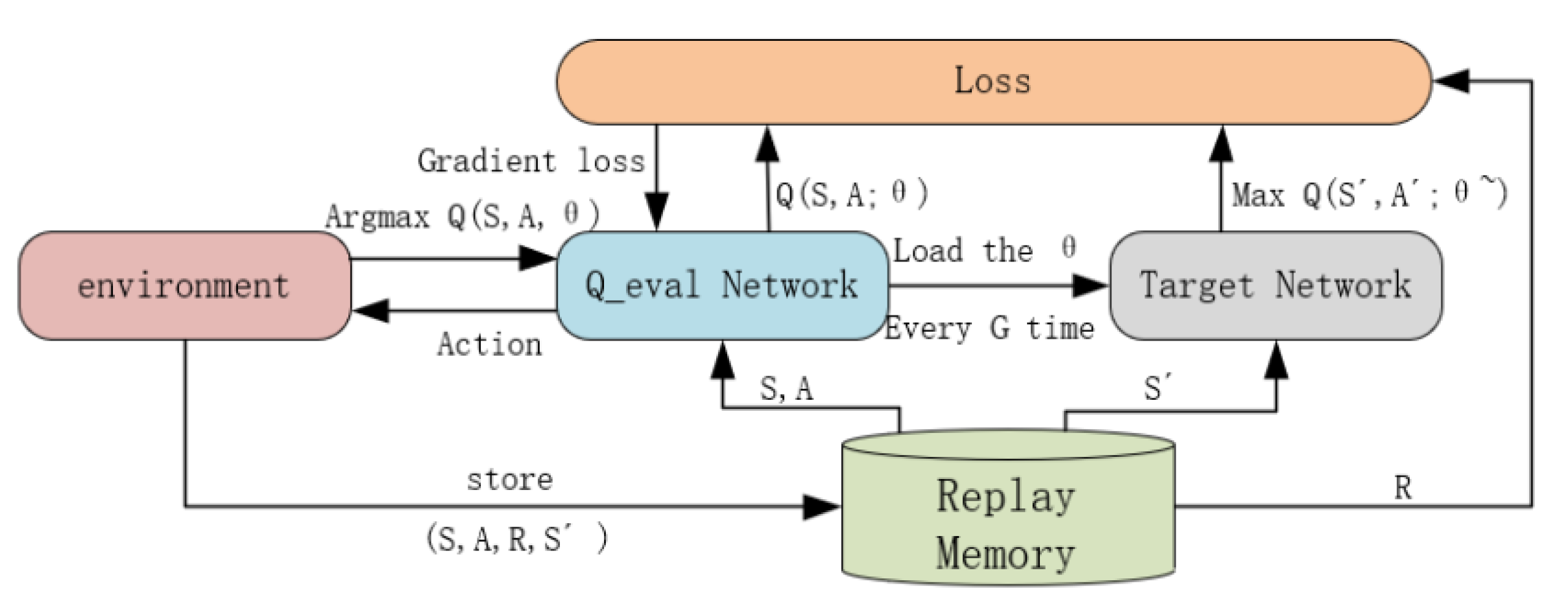
Therefore, the deep mind team proposed the deep Q network (DQN) based on an artificial neural network to make up for the defects of Q-learning. Both DQN and Q-learning are value-based algorithms in nature. DQN uses a neural network to calculate the Q-value of the corresponding action in a state and generates the Q-value corresponding to the action in a certain environment by fitting a function, instead of the Q-value table, thus avoiding the Q-value table occupying a lot of memory and querying the Q-value. The slowness of the table and other shortcomings, this method of using a deep neural network to fit a Q-value table is called deep reinforcement learning. The basic framework of DQN is shown in Figure 7. In the figure, S is the current state, A is the current action, R is the reward, $S^{\prime }$ is the next state, $A^{\prime }$ is the next action, $\theta$ is the parameter of the Q network, ${\theta }^{\prime }$ is the network parameters used to compute the target.

DQN is an improvement to Q-learning. It uses the characteristics of the artificial neural network to fit the Q-value table. On this basis, DQN also adds an experience replay pool to solve the problem of too high a correlation between samples. The experience replay pool stores A large amount of historical data, DQN does not update parameters immediately after performing an action like Q-learning, but stores a sample corresponding to the action $<s_t,a_t,r_t,a(t+1)>$ in Experience playback pool. When the acquired samples accumulate to a certain number, the training of the neural network starts. During training, a fixed number of samples are randomly selected from the experience replay pool for training. Since it is randomly selected, the probability of data drawn in the same round is very small, and the strong correlation between samples is broken, thus avoiding the need for neural networks. The local optimum problem arises from the instability. At the same time, labels are constructed through reward and punishment functions for neural network training. In addition, DQN also uses two neural networks with the same structure, one of which is a neural network with hysteresis parameters, namely the current value network and the target value network. The parameters of the Q-target (target value network) are the historical version of the Q-eval (current value network) neural network. Only the Q-eval neural network is trained. After a certain step, Q-target updates parameters that are the same as the parameters of Q-eval neural network, so as to reduce the connection between the current Q-value and the target Q-value, as well as to improve the convergence speed and stability of the neural network. The specific neural network parameter update formula is shown in Equation (8).

$$\left[\begin{array}{c}loss={(r_t+\gamma maxQ(s_{t+1},a^{\prime };{\theta }^{-})-Q(s_t,a_t;\theta ))}^2\end{array}\right]$$

(8)

In Equation (8), $Q(\ast ;{\theta }^{-})$ is the Q-target neural network. It does not need to train parameters through the Loss function, but only needs to update the parameters after a certain step size—$Q(\ast ;\theta )$ is the Q-eval neural network, and it directly gives the action that the agent needs to make through the environment. DQN uses the gradient descent method to train neural network parameters.

There are two artificial neural networks with the same structure, but different parameters in DQN. $Q(s_t,a_t;\theta )$ represents the value output by the current network, that is, Q-eval, which is used to output the optimal action in the current state. Additionally, $Q(s_{t+1},a^{\prime };{\theta }^{-})$ represents the output result of the target value network Q-target, so when the agent takes an action, it can update the parameters of Q-eval according to Equation (8), and after a certain step, iterate several times and copy the parameters of Q-eval to Q-target, thus completing a learning process.

Three existing improved DQN are combined to achieve the improvements proposed by this manuscript, including double DQN, dueling DQN, and prioritized experience replay (DQN).

3.3. Sampling Method

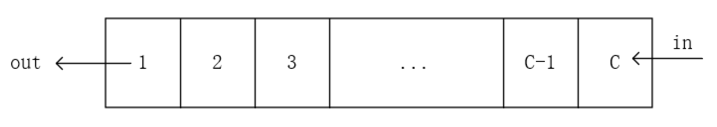
In DQN, the training samples in the playback memory pool are generated by the interaction between the agent and the environment and do not need to be provided by humans. During the interaction between the agent and the environment, new samples will be continuously generated and stored in the playback memory pool. When the number of memories stored in the playback memory pool reaches the size of the storage memory pool, the oldest sample will be deleted, and the new round is stored in the playback memory pool. Figure 8 shows the update method of the playback memory pool, which can ensure that the maximum capacity of the playback memory pool remains unchanged.

In DQN, the random sampling method is used to extract data from the playback memory pool for training, while in the full-coverage path planning, the repeated data that has less effect on the neural network update will have a high probability of being extracted as the neural network training data. It will slow down the convergence speed of the neural network. In this paper, the method of sumtree is used to extract data for learning.

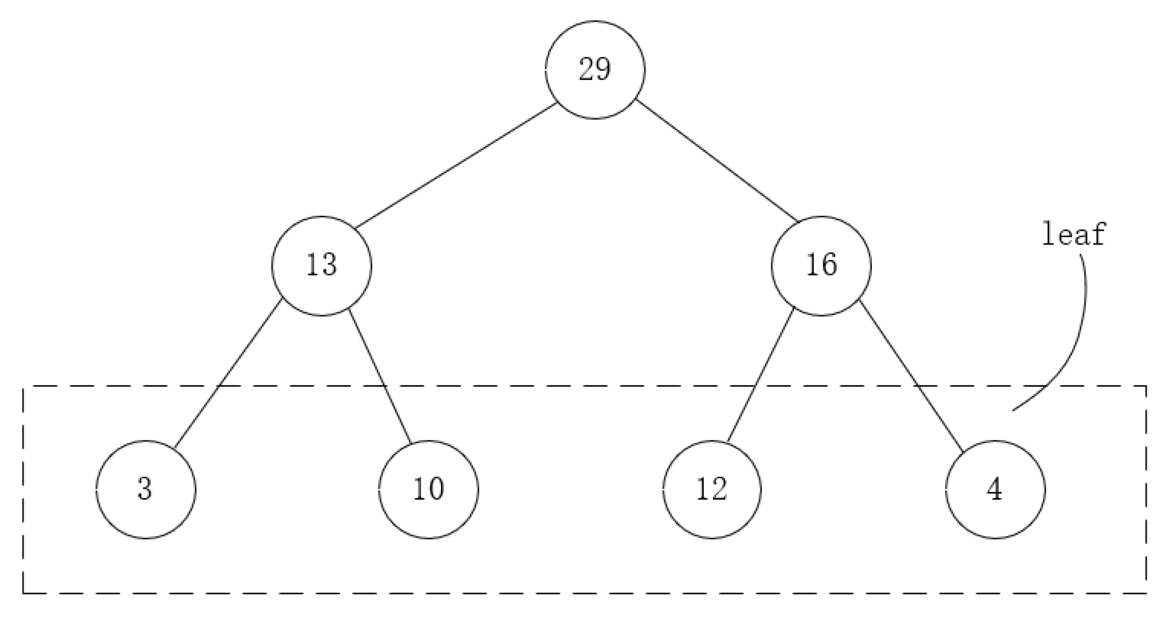
Sumtree is a binary tree structure, and its tree structure is only used to store the priority, and the extra data block is the data needed to be stored in the playback memory pool. The structure of sumtree is shown in Figure 9.

The leaf node stores the training priority value of each state, and this priority value is determined according to the value of its td-error. The larger the value of td-error, the higher the priority of selecting the memory. Its parent node is the sum of its two child nodes, and the value of the top-level node is the sum of the values of all the child nodes of the next layer. Each memory sample corresponds to a leaf node, and a certain amount of memory is extracted from the leaf nodes for the training each time. Saving data in a tree structure can greatly facilitate the sampling process, and it also ensures that each leaf node has a probability of being drawn, which greatly increases the convergence speed of the neural network.

In addition to replaying the memory pool, it is also necessary to optimize the loss function of the current value network to eliminate bias. The improved sample priority function is:

$$\left[\begin{array}{c}loss=1/m\sum _{j=1}{w}_j{(y_j-Q(s_j,a_j;\theta ))}^2\end{array}\right]$$

(9)

The definition of $w_j$ is shown in Equation (10).

$$\left[\begin{array}{c}{w}_j={(1/N\ast 1/P\left(j\right))}^{\beta }\end{array}\right]$$

(10)

Due to the use of priority to select samples, this will cause the distribution of samples to change, which will cause the sample model to converge to different values, that is, the neural network will be unstable. Therefore, importance sampling is used in this paper, which not only ensures that the probability of each sample being selected for training is different, in order to improve the training speed, but also ensures that its influence on the gradient descent of the neural network is the same, thereby ensuring that the neural network receives the same the result of. In Equation (10), N is the number of samples in the playback memory pool, and $\beta$ is a hyperparameter that needs to be set manually to offset the impact of changes in sample distribution.

3.4. Improvements Based on Action Selection

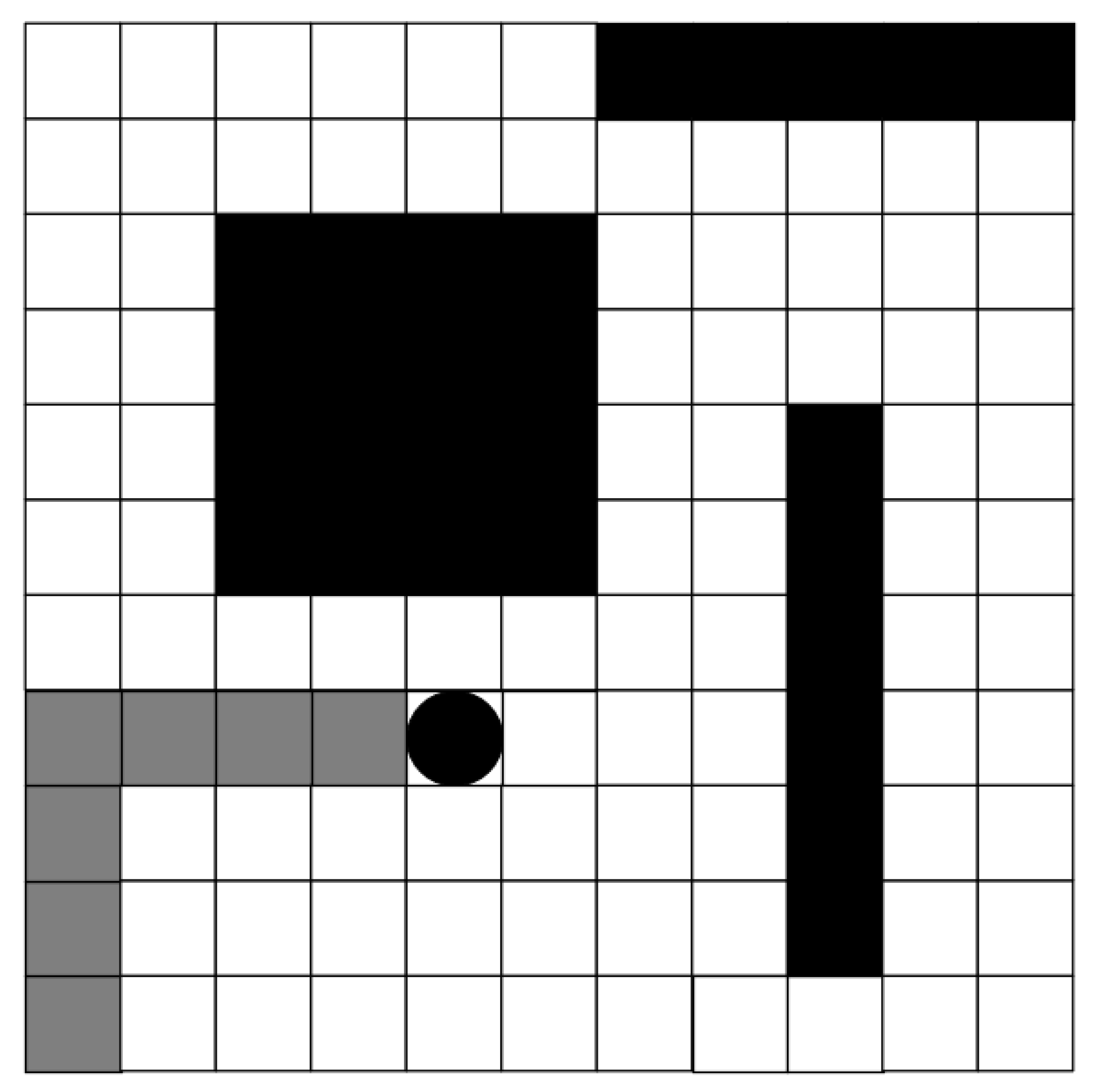
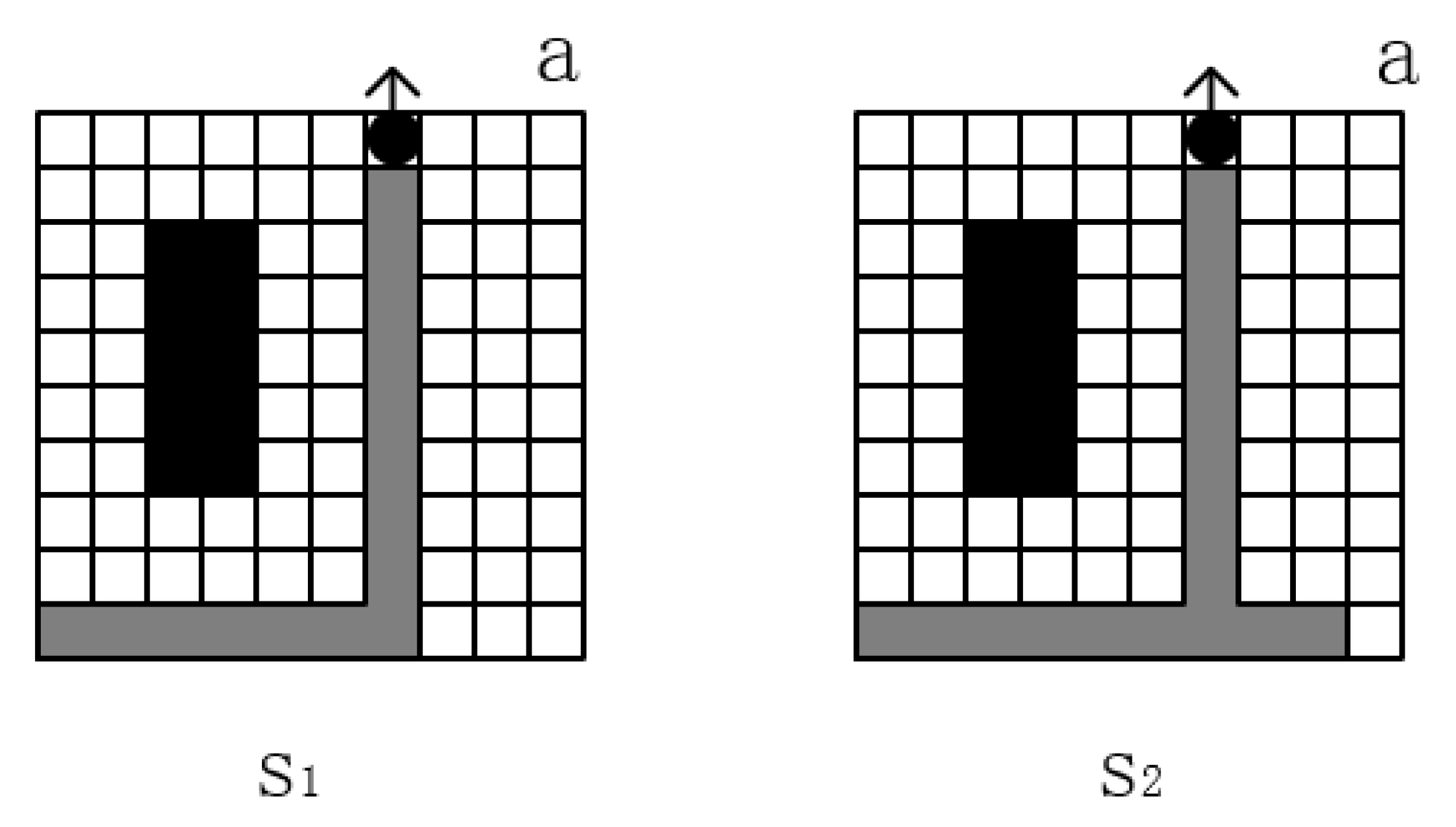
The USV explores the map under the strategy of the initial neural network. Since the parameters of the initial neural network are not trained or trained only a few times, the initial neural network is likely to give a strategy to collide with obstacles or go out of the map boundary. When the USV collides with an obstacle or walks out of the map boundary, the full-coverage task fails, and the USV returns to the initial position to try the next full-coverage path planning task, so the USV needs to undergo much training to avoid collision obstacles. The worst behavior is to avoid objects or go outside the boundaries of the map. Moreover, during the training process, even if the USV is in the same position, the state matrix of the map is different, due to the different previous behaviors. When the USV does the worst behavior, the reinforcement learning model will only make the state corresponding to this time. The Q-value of the action is reduced without extending it to all similar states, as shown in Figure 10.

As shown in Figure 10, state $s_1$ and state $s_2$ are two different states, black squares are obstacles, white squares are movable paths, gray squares are the paths traveled by USV, black circle is USV, and a represents the action taken by USV. When the USV makes a dangerous action only in state $s_1$, deep reinforcement learning will only train the neural network, so that Q–$eval(s_1,a)$ becomes smaller without making the value of Q–$eval(s_2,a)$ smaller, so that when the USV encounters the $s_2$ state, there is still a probability to choose the dangerous action a, which leads to the failure of the task.

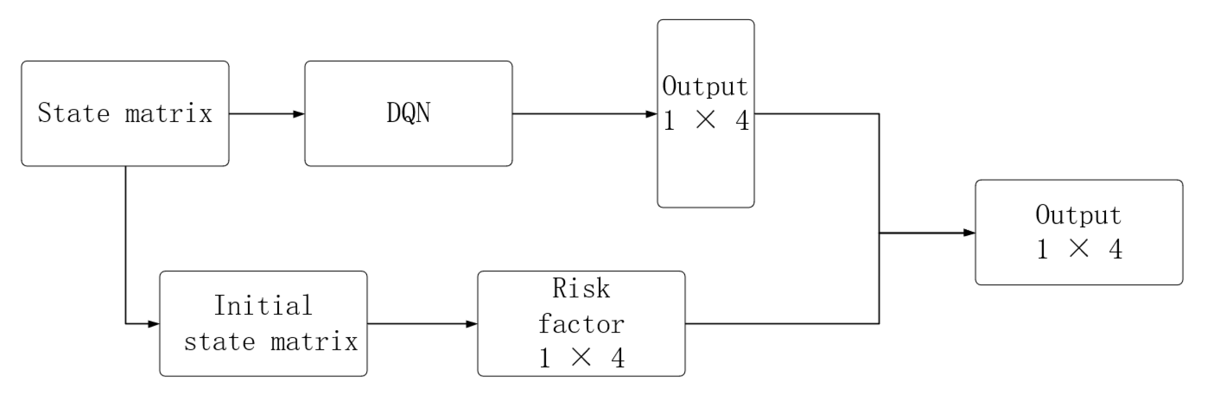
When humans perform similar tasks, they will actively avoid the above dangerous actions, so this paper proposes a method that can greatly reduce the probability of such dangerous actions. The policies for USVs are derived from current networks in deep reinforcement learning. The output of the current network is the Q-value of each action in the current environment. If you want to reduce the selection of dangerous actions, you only need to subtract a large number from the Q-value of the dangerous action. The specific implementation method is as follows.

Step 1: Assuming the size of the state map is n × n, first add −1 around the state map to represent the map boundary, as mentioned in the previous chapter. Then, convert the state map to the initial state, that is, change the values of all covered grids to 0.

Step 2: The position value in the state matrix of the USV is 7—find the position of the USV, and then multiply it by the surrounding elements based on the action value. For example, if the action value is up, it is multiplied by the element directly above the USV to obtain the danger of the action in this state. The four actions derive their corresponding dangers.

Step 3: Multiply the risk by the risk coefficient t, and then add it to the final output layer of DQN to form the final output. Its structure diagram is shown in Figure 11.

3.5. Design of the Reward Function

In order to improve the efficiency of full-coverage path planning, the USV should try to avoid repeatedly covering the covered area during the full-coverage path planning task and try to select the area that can cover the uncovered area every time an action is selected. So, the reward function initially defined by the text is shown in Equation (11).

$$r=\left\{\begin{array}{cc}\hfill 1& ,m(i,j)=0\hfill \\ \hfill 0& ,m(i,j)=1and{m}_{-1}(i\pm 1,j\pm 1)=1\hfill \\ \hfill -1& ,m(i,j)=1and\exists m_{-1}(i\pm ,j\pm 1)=0\hfill \\ \hfill -20& ,m(i,j)=-1ori,j<0ori,j>N\hfill \\ \hfill 20& ,done\hfill \end{array}\right.$$

(11)

where $m(i,j)$ represents the position in the grid map after the USV takes an action, and $m_{-1}(i\pm 1,j\pm 1)$ is the grid situation around the grid before the USV takes an action. When the USV enters an uncovered grid, it will obtain reward 1. When there is no uncovered grid around the USV, that is, all the grids around the USV have been covered or are obstacles, the USV takes no collision obstacles or actions that go out of the map’s borders and are rewarded with 0. When there is an uncovered grid around the USV, the vehicle still takes action to make itself enter the covered grid, and the reward is −1. When the vehicle takes an action and collides with an obstacle or goes out of the map boundary, it will obtain a reward of −20.

4. Simulation Results and Discussion

4.1. Simulation Platform

The simulation experiment in this paper runs in the Ubuntu 20.04 environment, using Python as the development language, and the parameters of the simulation platform are shown in

Table 2. Simulation platform.

Os	Language	CPU	GPU	RAM
Ubuntu 20.04	Python 3.8	intel10900	GTX2070	6 Gb

.

Based on the simulation platform we use, the duration of the proposed algorithm learning process usually takes one to two days. The duration of the learning process is limited by simulation platform, and a better simulation platform can significantly reduce learning time of the proposed algorithm. In order to verify the algorithm proposed in this paper, the size of the working environment of the USV in this paper is 20 × 20 m², which is divided into 11 × 11 grid maps.

4.2. Algorithm Simulation

In the simulation process, the above environmental parameters and DQN network model parameters are initialized first, and then a preprocessed grid map is constructed to record the grid map information and location information covered by the USV. Before each training starts, the position of the USV appears randomly on the grid map, and it is ensured that the position of the USV is not the position of the obstacle. During training, when the USV task is moved, the training will terminate, and the next training will begin. The conditions for task termination are that the USV collides with the map boundary or the obstacle grid, completes the full-coverage task, and the USV’s step size exceeds the set maximum step size. During the training process, each action will generate a sample, and the sample will be stored in the playback memory pool. When the number of samples reaches a certain level, the artificial neural network will be trained. When the training round reaches the set maximum training round, the training will end.

The simulation diagrams are shown in Figure 12, Figure 13, Figure 14 and Figure 15. Both the improved DQN proposed in this paper and the traditional boustrophedon method can complete the full-coverage path planning task well, and the coverage rate is 100%. The DQN and inner spiral coverage cannot complete the full-coverage path planning task. Their coverage rates are only 13% and 86%. As shown in Figure 13 and Figure 15, the coverage repetition rate of the improved DQN was 0.04%, while that of the boustrophedon method was 0.13%. Its final composite scores were 0.96 and 0.87 points, respectively. The effect of using the improved DQN-based full-coverage path planning algorithm is due to the traditional boustrophedon method.

Figure 16 shows the coverage of the full-coverage path planning algorithm using boustrophedon and the full-coverage path planning algorithm using the improved DQN. The red curve is the real-time coverage using boustrophedon, and the blue curve is the real-time coverage using the improved DQN full-coverage path planning. The horizontal axis is the step size, and the vertical axis is the coverage. From the real-time coverage map, it can be concluded that the improved DQN-based full-coverage path planning algorithm is more efficient than the boustrophedon method.

The loss function diagram of the improved DQN is shown in Figure 17, and its ordinate is the distance between the path and the optimal path, which can be obtained from Figure 4, Figure 5, Figure 6 and Figure 7. When the number of training times reaches 1000, the neural network has converged. The 1000 times at this point is not that the agent has performed 1000 tasks, but that 1000 times of memory are extracted from the playback memory pool for playback training, and the overall efficiency is high.

5. Conclusions

5.1. Main Conclusions and Findings

This paper proposes a raster map preprocessing method. Combined with the description and analysis of typical full-coverage path planning task scenarios, and further according to the characteristics of full-coverage path planning, we found the grids that cannot be covered by USVs and set them as obstacle grids.

To solve the problem of the low learning efficiency of traditional DQN, an improved action selection mechanism is proposed. This makes the failure rate of full-coverage path planning in the initial training phase lower. At the same time, the method of extracting memory training is improved, so that valuable data has a greater probability of being trained, and the efficiency of full-coverage of the area is improved.

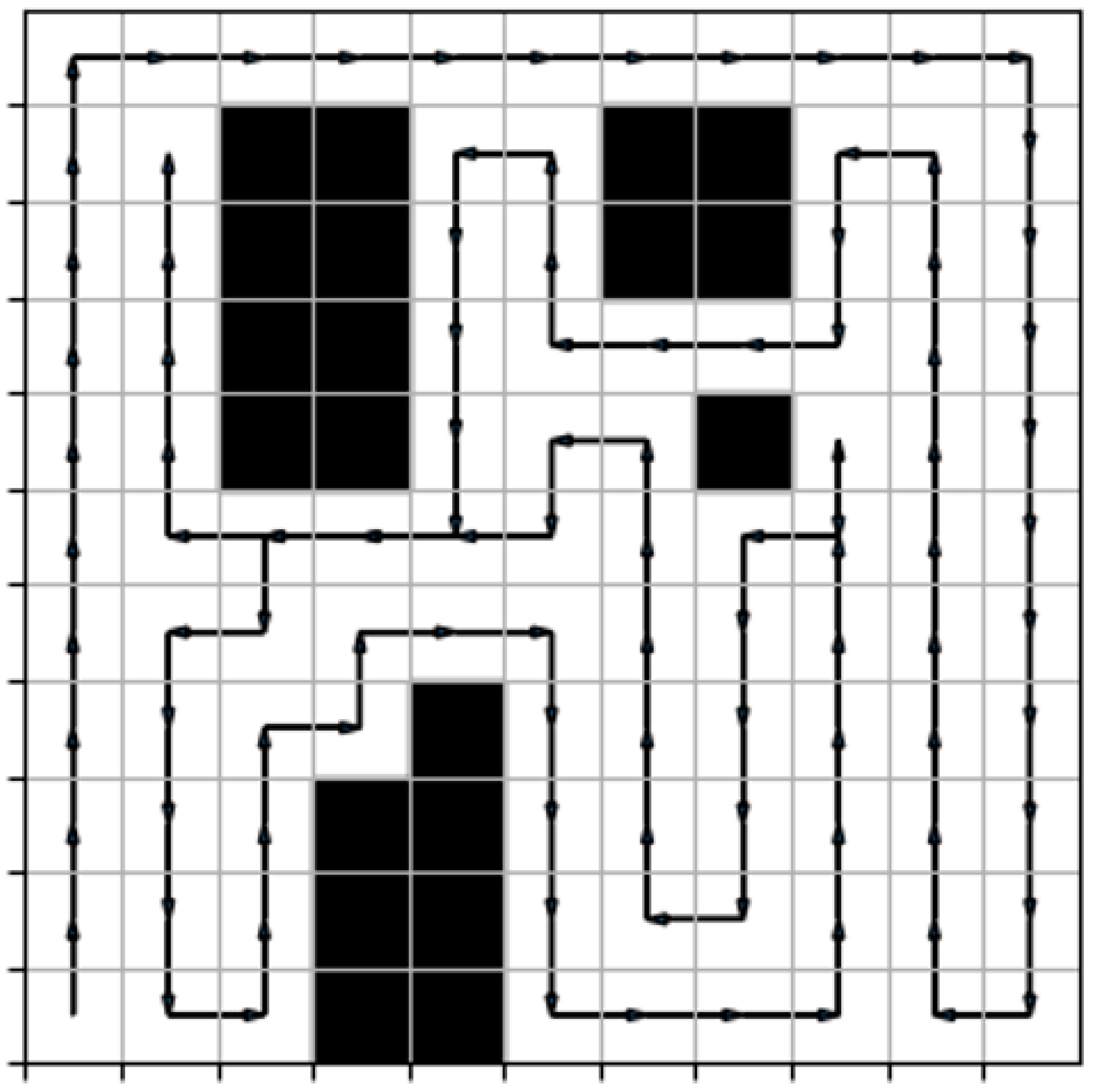
Simulation experiments show that the algorithm can effectively complete the full-coverage path planning task. The results show that, compared with the traditional full-coverage path planning algorithm, the proposed algorithm has good coverage rate. Compared with the boustrophedon and DQN algorithms, the performance of this algorithm on the coverage repetition rate is better, indicating that the performance of this algorithm is better.

5.2. Main Limitation of the Research

In modeling phase, the dynamical constraints and performance of the USV were not fully considered. The actual model of USV is more complex than the one in this study. This full-coverage path planning algorithm for USV might not have good performance in some situations.

5.3. Future Research Prospects

Considering economic factors, we usually want USVs to achieve full-coverage tasks efficiently at a low cost. To achieve this goal, the efficiency of path planning algorithms and their adaptability to different environments need to be improved.

In future work, the focus will be on the USV model and reward function, since the full-coverage path planning algorithm is affected by USV model and reward function when using simulation platform. At the same time, how to extend this algorithm to a complex actual environment with disturbances to obtain application value is also worth studying.