Research on Position Sensorless Control of RDT Motor Based on Improved SMO with Continuous Hyperbolic Tangent Function and Improved Feedforward PLL

Abstract

With the increasing use of electric propulsion ships, the emergence of the shaftless rim-driven thruster (RDT) as a revolutionary integrated motor thruster is gradually becoming an important development direction for green ships. The shaftless structure of RDTs leads to their dependence on position sensorless control techniques. In this study, a novel control algorithm using a composite sliding mode observer (SMO) with a modified feed-forward phase-locked loop (PLL) is presented for achieving high accuracy position and speed control of shaftless RDT motors. The deviation between the observed and actual currents is exploited to develop a current SMO to extract back electromotive force (back-EMF) errors. On this basis, a back-EMF observer is established to achieve accurate estimation of the back-EMF. The basic structure of the PLL was modified and incorporates a speed feedforward mechanism, which enhances the performance of rotor position estimation and facilitates bidirectional rotation. The stability of the algorithm has been verified in Matlab/Simulink for a range of steady-state, dynamic, and ship propeller loading conditions. Remarkably, the control algorithm boasts an impressive adjustment time of approximately 0.006 s and its position estimation error may be as low as 0.03 rad. Simulation results highlight the performance of the algorithm to achieve bidirectional rotation, while exhibiting fast convergence, minimal vibration, exceptional control accuracy, and robustness.

1. Introduction

Electric propulsion ships [1], underwater robots [2], unmanned surface vehicles [3,4], and other navigational vehicles [5] have undergone significant development in recent years, imposing more demands on propulsion systems. Electric propulsion systems are phasing out thermal propulsion systems due to their better control performance and higher control efficiency [6]. With the development of electric propulsion systems, integrated motors are increasingly being applied in a wide range of applications [7]. The shaftless rim-driven thruster (RDT) [8] is a revolutionary integrated motor thruster that merges propeller blades and motors to conserve cabin space, increase power density, motor efficiency, and hydrodynamic efficiency, as well as reduce system installation and manufacturing costs [9]. The introduction of the shaftless RDTs brings the electric propulsion ship systems more prominent features such as integration, electrification, intelligence, and flexibility [10]. As a typical complicated electromechanical system, the selection and control of the propulsion motor in the shaftless RDT are the most important considerations. Due to its great power density and efficiency, the permanent magnet synchronous motor (PMSM) is widely utilized in the field of propulsion motors [11]. The field-oriented control (FOC) [12] method of a PMSM requires precise real-time rotor position and speed information, which is commonly measured by mechanical position sensors installed on the rotor shaft, including shaft encoders, resolvers, and Hall sensors [13]. Because RDTs should operate in a harsh marine environment with high temperature, high humidity, and high salt for an extended period of time, shaftless RDTs cannot be equipped with conventional mechanical position sensors [14]. Simultaneously, removing the physical sensors from the control system can significantly enhance the system’s dependability and minimize motor production costs and size [15]. Consequently, it is necessary to develop the control algorithm of PMSM without a position sensor.

There are two types of PMSM position sensorless control strategies [16]: Back electromotive force (EMF) based mid-to-high speed method and saliency-tracking based zero-to-low speed approach. The motor dynamic model is utilized to obtain the back-EMF [17], which provides information on the rotor position and speed. The Kalman filter method [18], model adaptation method [19], Luenberger state observer [20], and sliding mode observer (SMO) [21] are the typical back-EMF-based methods.

The SMO approach has been widely adopted for the sensorless control of PMSM, owing to its straightforward construction, robustness against disturbances, and insensitivity to parameter variations [22]. However, the inherent switching characteristic of SMO gives rise to control discontinuity within the system, leading to undesirable chattering phenomena that compromise control precision and pose a risk to device integrity. The conventional SMO methods utilize the sign function as the sliding mode switching function [23], which exacerbates the problem of chattering due to the discontinuous nature of the sign function. Moreover, the back-EMF estimation by conventional SMO approaches is often plagued by high-frequency noise. As a result, one or more low-pass filters (LPF) are typically employed to extract the back-EMF signal. However, the use of LPFs introduces phase delays, necessitating position compensation based on the actual corner frequency and LPF cutoff frequency [24]. In response to these challenges, various research endeavors have been undertaken to address these issues and enhance the performance of the control system. In Ref. [25], a position-sensorless control method for PMSM was proposed, which utilized a SMO based on the variable boundary layer sigmoid function. The width of the boundary layer was adjusted based on the velocity to effectively address the chattering issue. However, this method used a LPF, which resulted in a phase shift of the system state and reduced the estimation accuracy. To solve the phase delay problem. In Ref. [26], a cascade low-pass filter (LPF) with a variable cut-off frequency is proposed to mitigate chattering. In addition, a variable phase delay compensation is applied to counterbalance the phase shift introduced by the LPF across the speed range. Although the LPF with delay compensation strategy has demonstrated its effectiveness in improving the performance of PMSMs, its topological complexity poses challenges for practical implementation. In Ref. [27], the authors proposed a new approach for rotor position estimation in permanent magnet synchronous motors (PMSMs) using a hyperbolic function-based SMO. Unlike conventional SMOs, the proposed approach eliminates the need for a low-pass filter (LPF) and angle compensator. The previous study proposed a method to reduce chattering in sliding mode observers (SMOs) by utilizing a continuous switching function to construct a transition boundary layer and generate a quasi-SMO. However, the thickness of the boundary layer had a significant impact on the performance of the SMO. A narrow boundary layer range improved the approach speed of the sliding mode motion, but introduced chattering and harmonic distortion in the back-EMF. Conversely, a wide boundary layer reduced chattering but weakened the robustness of the control system by decreasing the approximation speed. Thus, regulating the width of the boundary layer appropriately based on the continuous switching function was necessary to enhance the performance of the control system while minimizing the chattering.

Sensorless control algorithms traditionally employ the inverse tangent function to extract rotor position information from the back-EMF for motor speed calculation. However, the rotor position estimation approach that utilizes the inverse tangent function introduces high-frequency harmonics into the division operation, leading to an amplification of high-frequency harmonics that can cause significant errors in rotor position estimation. In Ref. [28], a current pre-compensation scheme based on a double sampling strategy with one switching cycle was proposed to improve the accuracy of position estimation and motor control performance by compensating for the computational delay. However, this technique significantly increased the computing complexity of the control system. To address this issue, many researchers have proposed using phase-locked loop (PLL) to extract rotor position and velocity information [29], which provides a simpler and more efficient alternative for sensorless control. PLL usually consists of three parts: phase detector (PD), loop filter (LF), and voltage-controlled oscillator (VCO). The PLL described in the preceding work was referred to the traditional PLL. The conventional phase-locked loop (PLL) has been shown to enhance the reliability of rotor position estimation. However, it is only appropriate for estimating position information when the motor moves in one direction with uniform parameters. Upon motor reversal, a position deviation of 180° arises, causing imprecise estimation of the system position. In Ref. [13], the authors introduced a position estimation technique for the sensorless control of a PMSM that utilized a PLL structure with a tangent function. This enhanced PLL provided reliable rotor position estimation during both forward and backward rotation, catering to the frequent forward and reverse RDT rotation requirements. However, due to its reliance on a tangent function, the technique was vulnerable to noise interference, leading to imprecise location estimation. An often overlooked problem with conventional phase-locked loops (PLLs) is their inability to quickly track rotor position during acceleration and deceleration. Additionally, maintaining a zero steady-state error is challenging, and sudden changes in velocity can result in significant position estimation errors, leading to tracking failures.

To address the aforementioned issues, a position-sensorless algorithm for PMSM is proposed in this study, based on a composite SMO and a feedforward PLL. The composite SMO comprises a modified current SMO and a back-EMF observer. The modified current SMO adopts a continuous hyperbolic tangent function to replace the discontinuous sign function, which reduces the SMO chatter. This SMO extracts the counter-electromotive force error, which is much smaller in amplitude than the counter-electromotive force, so a smaller SMO gain factor can be set to further weaken the chattering. The back-EMF observer is constructed based on the back-EMF model, which replaces the traditional LPF and avoids phase delay while greatly improving the observation accuracy of the back-EMF. The proposed PLL with rotor speed feedforward compensation enhances the tracking stability and position extraction accuracy, while maintaining the reliability of position extraction when the motor rotates in both directions. The stability of the composite SMO and PLL is verified through simulations under steady-state, dynamic, ship propeller load, and external random disturbance conditions. The experimental results demonstrate that the algorithm features fast convergence, small jitter, high control accuracy, and strong robustness compared with conventional algorithms. There are two main highlights in this paper:

(1)

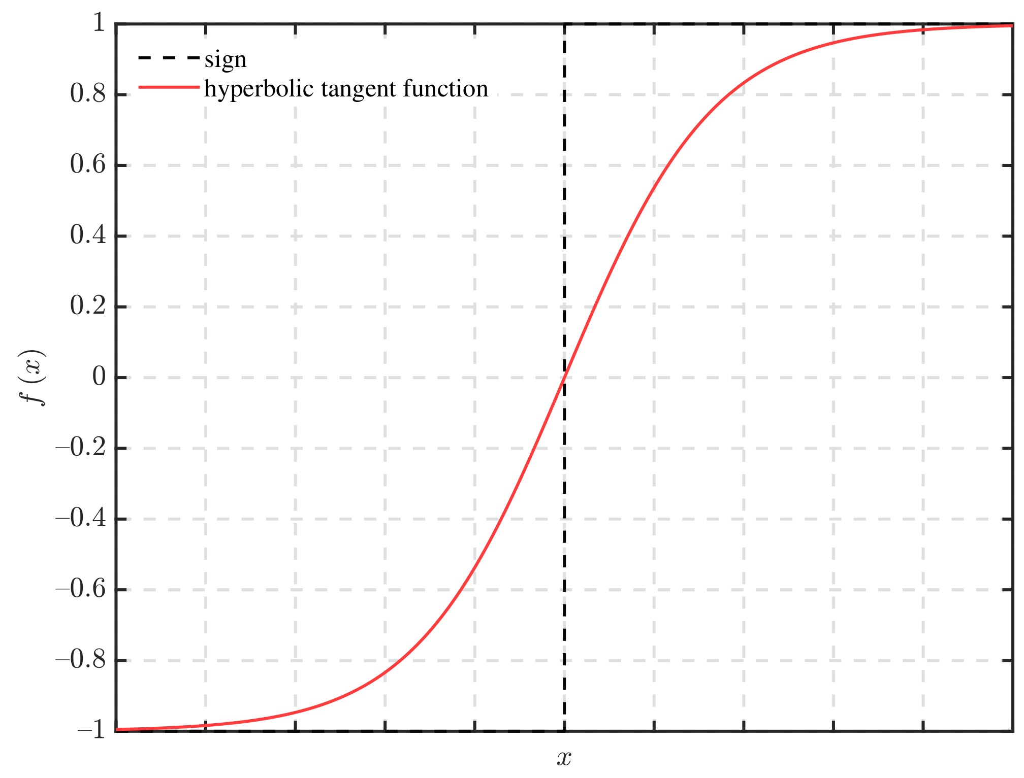
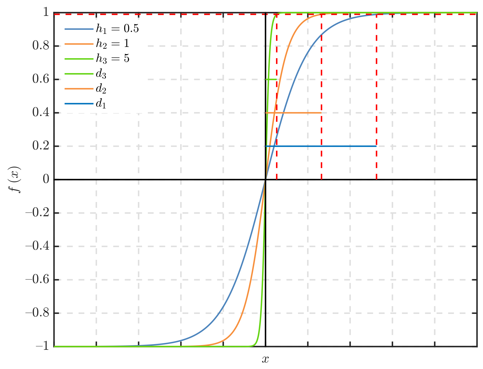
This study addresses SMO chattering by replacing the sign function with a continuous hyperbolic tangent function and selecting an appropriate boundary layer width. An observer based on the back-EMF model is developed to eliminate the LPF, reduce phase delay, and enhance the back-EMF signal estimation precision;

(2)

Through optimization of the traditional PLL structure and the addition of feedforward compensation, this study has successfully realized position extraction during bi-directional rotation of the motor, while significantly improving the accuracy of position extraction during acceleration and deceleration.

The remainder of this paper is organized as follows: In Section 2, the mathematical model of PMSM is presented. Section 3 proposes the improved SMO and counter-electromotive force observer, and their stability is proven. Section 4 analyzes the limitations of the conventional PLL and presents the design of the improved feedforward PLL, along with a discussion of its stability. Simulation results under different conditions are presented in Section 5 to demonstrate the superiority and reliability of the proposed algorithm. Finally, Section 6 concludes the paper.

2. PMSM Mathematical Model

In the $d-q$ coordinate system, the mathematical model of the surface-mounted PMSM is shown in Equation (1), in which iron saturation, flux leakage, eddy current, and hysteresis losses can be ignored.

$$\begin{array}{c}\hfill \left\{\begin{array}{cc}\hfill & u_d=R_s{i}_d+L_s\frac{d{i}_d}{dt}-{\omega }_e{L}_s{i}_q\hfill \\ \hfill & u_q=R_s{i}_q+L_s\frac{d{i}_q}{dt}+{\omega }_e{L}_s{i}_d+{\omega }_e{\psi }_f\hfill \end{array}\right.\end{array}$$

(1)

where $u_d$, $u_q$, $i_d$, $i_q$ represent the voltage and current in the corresponding coordinate system, respectively. $R_{\mathrm{s}}$, $L_s$ represent the stator resistance and stator inductance, respectively. ${\psi }_f$ represents the permanent magnet flux linkage, and ${\omega }_e$ represents the electrical angular velocity. Equation (1) can be converted to a stationary $\alpha$−$\beta$ coordinate system using the coordinate transformation as follows.

$$\begin{array}{c}\hfill \left\{\begin{array}{cc}\hfill & u_{\alpha }=R_s{i}_{\alpha }+L_s\frac{d{i}_{\alpha }}{dt}+e_{\alpha }\hfill \\ \hfill & u_{\beta }=R_s{i}_{\beta }+L_s\frac{d{i}_{\beta }}{dt}+e_{\beta }\hfill \end{array}\right.\end{array}$$

(2)

where $u_{\alpha }$, $u_{\beta }$, $i_{\alpha }$, $i_{\beta }$, $e_{\alpha }$, $e_{\beta }$ represent the voltage, current, and back-EMF in the corresponding coordinate system, respectively. The back-EMF is described as

$$\begin{array}{c}\hfill \left\{\begin{array}{cc}\hfill & e_{\alpha }=-{\psi }_f{\omega }_{e}sin\left({\theta }_e\right)\hfill \\ \hfill & e_{\beta }={\psi }_f{\omega }_{e}cos\left({\theta }_e\right)\hfill \end{array}\right.\end{array}$$

(3)

where ${\theta }_e$ is the electrical angle and the ${\omega }_e$ can be expressed as

$${\omega }_e=\frac{1}{{\psi }_f}\sqrt{(e_{\alpha }^2+e_{\beta }^2)}$$

(4)

From Equation (3), it can be seen that the back-EMF contains information regarding the position and angular velocity of the motor rotor. The exact observation of the motor back-EMF is, thus, the foundation of the position-sensorless control algorithm.

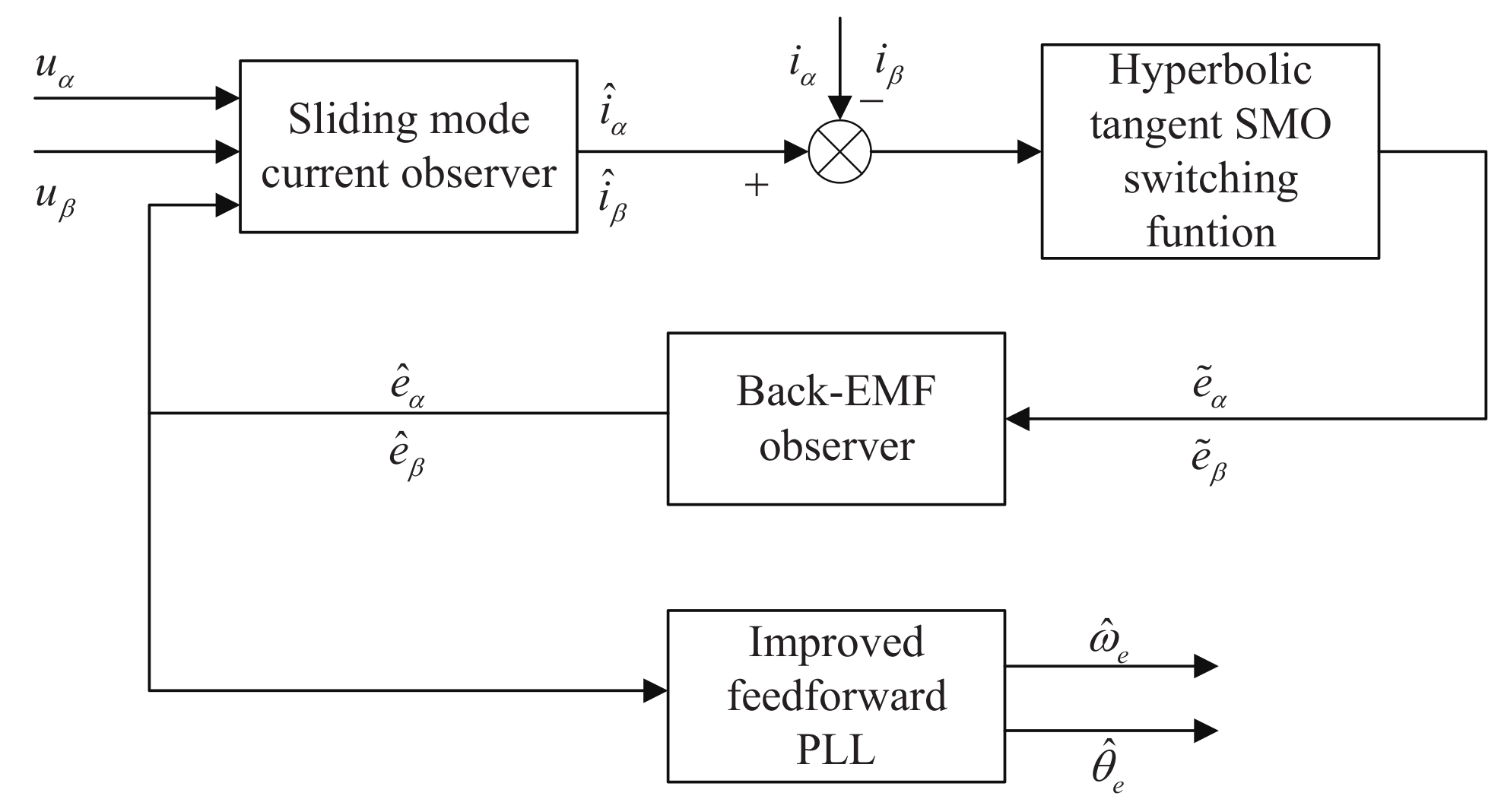
3. SMO Design for PMSM Rotor Position Estimation

In this paper, based on the mathematical model of PMSM, an improved SMO is constructed based on the error between the actual current $i_{\alpha }$, $i_{\beta }$ and the observed current ${\widehat{i}}_{\alpha }$, ${\widehat{i}}_{\beta }$ to obtain the back-EMF errors ${\tilde{e}}_{\alpha }$, ${\tilde{e}}_{\beta }$. Next, the back-EMF observer is constructed based on the back-EMF model, and the back-EMF ${\widehat{e}}_{\alpha }$, ${\widehat{e}}_{\beta }$ is the output.

According to Equation (2), the expression for the current can be written as

$$\begin{array}{c}\hfill \left\{\begin{array}{cc}\hfill & \frac{d{i}_{\alpha }}{dt}=\frac{u_{\alpha }-R_s{i}_{\alpha }-e_{\alpha }}{L_s}\hfill \\ \hfill & \frac{d{i}_{\beta }}{dt}=\frac{u_{\beta }-R_s{i}_{\beta }-e_{\beta }}{L_s}\hfill \end{array}\right.\end{array}$$

(5)

Define ${\tilde{i}}_{\alpha }$, ${\tilde{i}}_{\beta }$ as the current estimation error of SMO with the following expression:

$$\begin{array}{c}\hfill \left\{\begin{array}{cc}\hfill & {\tilde{i}}_{\alpha }={\widehat{i}}_{\alpha }-i_{\alpha }\hfill \\ \hfill & {\tilde{i}}_{\beta }={\widehat{i}}_{\beta }-i_{\beta }\hfill \end{array}\right.\end{array}$$

(6)

where ${\widehat{i}}_{\alpha }$, ${\widehat{i}}_{\beta }$ are SMO estimated currents. Based on the theory of the sliding mode variable structure, the sliding surface is chosen as

$$\begin{array}{c}\hfill s\left({\tilde{i}}_s\right)=\left[\begin{array}{c}{s}_{\alpha }\left({\tilde{i}}_{\alpha }\right)\hfill \\ s_{\beta }\left({\tilde{i}}_{\beta }\right)\hfill \end{array}\right]={\tilde{i}}_s+\mu \underset{0}{\overset{t}{\int }}{\tilde{i}}_{s}d\tau \end{array}$$

(7)

where ${\tilde{i}}_s={\left[\begin{array}{cc}{\tilde{i}}_{\alpha }& {\tilde{i}}_{\beta }\end{array}\right]}^{\mathrm{T}}$, $\mu$ is a constant and satisfies $0<\mu <R_s/L_s$.

According to the mathematical model of PMSM, the SMO is established as follows:

$$\begin{array}{c}\hfill \left\{\begin{array}{cc}\hfill & \frac{d{\widehat{i}}_{\alpha }}{dt}=\frac{u_{\alpha }-R_s{\widehat{i}}_{\alpha }-{\widehat{e}}_{\alpha }-\lambda ·F\left(S_{\alpha }\left({\tilde{i}}_{\alpha }\right)\right)}{L_s}\hfill \\ \hfill & \frac{d{\widehat{i}}_{\beta }}{dt}=\frac{u_{\beta }-R_s{\widehat{i}}_{\beta }-{\widehat{e}}_{\beta }-\lambda ·F\left(S_{\beta }\left({\tilde{i}}_{\beta }\right)\right)}{L_s}\hfill \end{array}\right.\end{array}$$

(8)

where $F\left(·\right)$ is the sliding mode switching function and $\lambda$ is the sliding mode gain.

Due to the discontinuous character of the sign function, the back-EMF estimation generates significant chattering. In order to reduce the chattering phenomenon of SMO, the continuous hyperbolic tangent function is used instead of the sign function. The images of the sign function and hyperbolic tangent function are shown in Figure 1. The hyperbolic tangent function is demonstrated below:

$$\begin{array}{c}\hfill F\left(s\right)=\frac{e^{hs}-e^{-hs}}{e^{hs}+e^{-hs}}\end{array}$$

(9)

Figure 2 depicts the hyperbolic tangent function with different values of h, which shows that the boundary layer width d is inversely proportional to the coefficient h. The magnitude of h is related to SMO chattering. The chattering of the state variable trajectory in SMO reduces as h decreases. When it increases, the approximation speed of the state variable improves, but if it is too large, SMO robustness is compromised. Therefore, the balance between the robustness of SMO and suppression of chattering needs to be considered when choosing h.

The current observation error equation can be obtained by subtracting Equation (5) from Equation (8),

$$\begin{array}{c}\hfill \left\{\begin{array}{cc}\hfill & \frac{d{\tilde{i}}_{\alpha }}{dt}=\frac{-R_s{\tilde{i}}_{\alpha }-{\tilde{e}}_{\alpha }-\lambda ·F\left(S_{\alpha }\left({\tilde{i}}_{\alpha }\right)\right)}{L_s}\hfill \\ \hfill & \frac{d{\tilde{i}}_{\beta }}{dt}=\frac{-R_s{\tilde{i}}_{\beta }-{\tilde{e}}_{\beta }-\lambda ·F\left(S_{\beta }\left({\tilde{i}}_{\beta }\right)\right)}{L_s}\hfill \end{array}\right.\end{array}$$

(10)

According to the sliding mode equivalence principle, we may derive:

$$\begin{array}{c}\hfill \left\{\begin{array}{cc}\hfill & {\tilde{e}}_{\alpha }=-\lambda ·F\left(S_{\alpha }\left({\tilde{i}}_{\alpha }\right)\right)+(\mu L_s-R_s){\tilde{i}}_{\alpha }\hfill \\ \hfill & {\tilde{e}}_{\beta }=-\lambda ·F\left(S_{\beta }\left({\tilde{i}}_{\beta }\right)\right)+(\mu L_s-R_s){\tilde{i}}_{\beta }\hfill \end{array}\right.\end{array}$$

(11)

Theorem 1.

Consider the closed-loop system, which consists of Equation (2) with environmental disturbances. Assume that Equation (8), Equation (21), and PLL are stable. When the system parameters are set to satisfy $0<\mu <R_s/L_s$ and $\lambda >max\left(\right|{\tilde{e}}_{\alpha }|,|{\tilde{e}}_{\beta }\left|\right)$, the current observation error, back-EMF estimation error, position estimation error, and velocity estimation error converge asymptotically to zero.

Proof of Theorem 1.

The Lyapunov function is chosen as follows,

$$\begin{array}{c}\hfill V\left({\tilde{i}}_s\right)=\frac{1}{2}S{\left({\tilde{i}}_s\right)}^{T}S\left({\tilde{i}}_s\right)\end{array}$$

(12)

The derivative of the above equation yields,

$$\begin{array}{c}\hfill \begin{array}{cc}\hfill \dot{V}\left({\tilde{i}}_s\right)& =S{\left({\tilde{i}}_s\right)}^T\dot{S}\left({\tilde{i}}_s\right)\hfill \\ \hfill & =S_{\alpha }\left({\tilde{i}}_{\alpha }\right){\dot{S}}_{\alpha }\left({\tilde{i}}_{\alpha }\right)+S_{\beta }\left({\tilde{i}}_{\beta }\right){\dot{S}}_{\beta }\left({\tilde{i}}_{\beta }\right)\hfill \\ \hfill & =S_{\alpha }\left({\tilde{i}}_{\alpha }\right)[\{{\dot{\tilde{i}}}_{\alpha }+\mu {\tilde{i}}_{\alpha }]+S_{\beta }\left({\tilde{i}}_{\beta }\right)[\{{\dot{\tilde{i}}}_{\beta }+\mu {\tilde{i}}_{\beta }]\hfill \\ \hfill & ={\dot{V}}_{\alpha }\left({\tilde{i}}_{\alpha }\right)+{\dot{V}}_{\beta }\left({\tilde{i}}_{\beta }\right)\hfill \end{array}\end{array}$$

(13)

where ${\dot{V}}_{\alpha }\left({\tilde{i}}_{\alpha }\right)=S_{\alpha }\left({\tilde{i}}_{\alpha }\right)[{\dot{\tilde{i}}}_{\alpha }+\mu {\tilde{i}}_{\alpha }]$ and ${\dot{V}}_{\beta }\left({\tilde{i}}_{\beta }\right)=S_{\beta }\left({\tilde{i}}_{\beta }\right)[{\dot{\tilde{i}}}_{\beta }+\mu {\tilde{i}}_{\beta }]$.

According to ${\dot{V}}_{\alpha }\left({\tilde{i}}_{\alpha }\right)$ and Equation (10) it can be derived that

$$\begin{array}{c}\hfill \begin{array}{cc}\hfill {\dot{V}}_{\alpha }\left({\tilde{i}}_{\alpha }\right)& =S_{\alpha }\left({\tilde{i}}_{\alpha }\right)[{\dot{\tilde{i}}}_{\alpha }+\mu {\tilde{i}}_{\alpha }]\hfill \\ \hfill & =S_{\alpha }\left({\tilde{i}}_{\alpha }\right)[-\frac{R_s}{L_s}{\tilde{i}}_{\alpha }-\frac{1}{L_s}{\tilde{e}}_{\alpha }-\frac{1}{L_s}\lambda ·F\left(S_{\alpha }\left({\tilde{i}}_{\alpha }\right)\right)+\mu {\tilde{i}}_{\alpha }]\hfill \\ \hfill & =(\mu -\frac{R_s}{L_s}){\tilde{i}}_{\alpha }{S}_{\alpha }\left({\tilde{i}}_{\alpha }\right)-\frac{S_{\alpha }\left({\tilde{i}}_{\alpha }\right)}{L_s}({\tilde{e}}_{\alpha }+\lambda ·F\left(S_{\alpha }\left({\tilde{i}}_{\alpha }\right)\right))\hfill \end{array}\end{array}$$

(14)

According to Equation (7) and $0<\mu <R_s/L_s$ we can get the first term of the above equation as

$$\begin{array}{c}\hfill (\mu -\frac{R_s}{L_s}){\tilde{i}}_{\alpha }{S}_{\alpha }\left({\tilde{i}}_{\alpha }\right)=(\mu -\frac{R_s}{L_s})({{\tilde{i}}_{\alpha }}^2+{\tilde{i}}_{\alpha }\mu \underset{0}{\overset{t}{\int }}{\tilde{i}}_{\alpha }d\tau )\le 0\end{array}$$

(15)

When $\lambda >|{\tilde{e}}_{\alpha }|$, the second term of Equation (14) satisfies

$$\begin{array}{c}\hfill -\frac{S_{\alpha }\left({\tilde{i}}_{\alpha }\right)}{L_s}({\tilde{e}}_{\alpha }+\lambda ·F\left(S_{\alpha }\left({\tilde{i}}_{\alpha }\right)\right))<0\end{array}$$

(16)

In accordance with the aforementioned derivation, we may obtain

$$\begin{array}{c}\hfill \begin{array}{cc}\hfill {\dot{V}}_{\alpha }\left({\tilde{i}}_{\alpha }\right)& =(\mu -\frac{R_s}{L_s}){\tilde{i}}_{\alpha }{S}_{\alpha }\left({\tilde{i}}_{\alpha }\right)-\frac{S_{\alpha }\left({\tilde{i}}_{\alpha }\right)}{L_s}({\tilde{e}}_{\alpha }+\lambda ·F\left(S_{\alpha }\left({\tilde{i}}_{\alpha }\right)\right))<0\hfill \end{array}\end{array}$$

(17)

Likewise, when $\lambda >|{\tilde{e}}_{\beta }|$, we may derive

$$\begin{array}{c}\hfill \begin{array}{cc}\hfill {\dot{V}}_{\beta }\left({\tilde{i}}_{\beta }\right)& =(\mu -\frac{R_s}{L_s}){\tilde{i}}_{\beta }{S}_{\beta }\left({\tilde{i}}_{\beta }\right)-\frac{S_{\beta }\left({\tilde{i}}_{\beta }\right)}{L_s}({\tilde{e}}_{\beta }+\lambda ·F\left(S_{\beta }\left({\tilde{i}}_{\beta }\right)\right))<0\hfill \end{array}\end{array}$$

(18)

Thus, when $\lambda >max\left(\right|{\tilde{e}}_{\alpha }|,|{\tilde{e}}_{\beta }\left|\right)$, we obtain

$$\begin{array}{c}\hfill \dot{V}\left({\tilde{i}}_s\right)={\dot{V}}_{\alpha }\left({\tilde{i}}_{\alpha }\right)+{\dot{V}}_{\beta }\left({\tilde{i}}_{\beta }\right)<0\end{array}$$

(19)

This shows that the sliding mode surface as depicted in Equation (7) is reachable, therefore the SMO is stable and can accurately obtain the back-EMF error as described in Equation (11). The conventional SMO sliding mode gain needs to satisfy $\lambda >max\left(\right|e_{\alpha }|,|e_{\beta }\left|\right)$, while the improved SMO only needs to satisfy $\lambda >max\left(\right|{\tilde{e}}_{\alpha }|,|{\tilde{e}}_{\beta }\left|\right)$. Obviously, the back-EMF error is smaller than the back-EMF. Therefore, the sliding mode gain of the improved SMO setting is significantly smaller than that of the conventional SMO, which can weaken the sliding mode chattering. □

The aforementioned SMO is capable of generating an equivalent back-EMF error signal, but this signal still contains a high-frequency component and cannot be utilized directly to extract rotor position information. Most conventional methods use LPF for filtering, but this introduces a phase delay, which impacts the subsequent extraction of rotor position information. This work employs the back-EMF model to construct the observer, extract the back-EMF signal, and then use PLL to estimate the rotor position and speed. Since the change rate of motor speed is significantly smaller than that of the stator current, assuming ${\dot{\omega }}_e=0$, the back-EMF model of PMSM can be expressed as

$$\begin{array}{c}\hfill \left\{\begin{array}{cc}\hfill & \frac{d{e}_{\alpha }}{dt}=-{\psi }_f{\dot{\omega }}_{e}sin{\theta }_e-{\psi }_f{\omega }_{e}cos{\theta }_e\frac{d{\theta }_e}{dt}=-{\omega }_e{e}_{\beta }\hfill \\ \hfill & \frac{d{e}_{\beta }}{dt}={\psi }_f{\dot{\omega }}_{e}cos{\theta }_e-{\psi }_f{\omega }_{e}sin{\theta }_e\frac{d{\theta }_e}{dt}={\omega }_e{e}_{\alpha }\hfill \end{array}\right.\end{array}$$

(20)

Based on the above equation, the back-EMF observer is established as

$$\begin{array}{c}\hfill \left\{\begin{array}{cc}\hfill & \frac{d{\widehat{e}}_{\alpha }}{dt}=-{\widehat{\omega }}_e{\widehat{e}}_{\beta }-m{\tilde{e}}_{\alpha }\hfill \\ \hfill & \frac{d{\widehat{e}}_{\beta }}{dt}={\widehat{\omega }}_e{\widehat{e}}_{\alpha }-m{\tilde{e}}_{\beta }\hfill \\ \hfill & \frac{d{\widehat{\omega }}_e}{dt}={\tilde{e}}_{\alpha }{\widehat{e}}_{\beta }-{\tilde{e}}_{\beta }{\widehat{e}}_{\alpha }\hfill \end{array}\right.\end{array}$$

(21)

where m is the observer gain, and $m>0$. The error equation can be obtained by subtracting Equation (20) from Equation (21),

$$\begin{array}{c}\hfill \left\{\begin{array}{cc}\hfill & \frac{d{\tilde{e}}_{\alpha }}{dt}=-{\tilde{\omega }}_e{\widehat{e}}_{\beta }-{\omega }_e{\tilde{e}}_{\beta }-m{\tilde{e}}_{\alpha }\hfill \\ \hfill & \frac{d{\tilde{e}}_{\beta }}{dt}={\tilde{\omega }}_e{\widehat{e}}_{\alpha }+{\omega }_e{\tilde{e}}_{\alpha }-m{\tilde{e}}_{\beta }\hfill \\ \hfill & \frac{d{\tilde{\omega }}_e}{dt}={\tilde{e}}_{\alpha }{\widehat{e}}_{\beta }-{\tilde{e}}_{\beta }{\widehat{e}}_{\alpha }\hfill \end{array}\right.\end{array}$$

(22)

Theorem 2.

Considering that the change rate of motorspeed is significantly smaller than that of the stator current, assume that ${\dot{\omega }}_e=0$. When the back-EMF observer is stable, the back-EMF error converges to zero and the back-EMF observation can be obtained accurately.

Proof of Theorem 2.

To verify the stability of the back-EMF observer, the Lyapunov function is chosen as

$$\begin{array}{c}\hfill V=\frac{{\tilde{e}}_{\alpha }^2+{\tilde{e}}_{\beta }^2+{\tilde{\omega }}_e^2}{2}\end{array}$$

(23)

Derivation of the above equation yields

$$\begin{array}{c}\hfill \begin{array}{cc}\hfill \dot{V}& ={\tilde{e}}_{\alpha }{\dot{\tilde{e}}}_{\alpha }+{\tilde{e}}_{\beta }{\dot{\tilde{e}}}_{\beta }+{\tilde{\omega }}_e{\dot{\tilde{\omega }}}_e\hfill \\ \hfill & ={\tilde{e}}_{\alpha }(-{\tilde{\omega }}_e{\widehat{e}}_{\beta }-{\omega }_e{\tilde{e}}_{\beta }-m{\tilde{e}}_{\alpha })+{\tilde{e}}_{\beta }({\tilde{\omega }}_e{\widehat{e}}_{\alpha }+{\omega }_e{\tilde{e}}_{\alpha }-m{\tilde{e}}_{\beta })+{\tilde{\omega }}_e({\tilde{e}}_{\alpha }{\widehat{e}}_{\beta }-{\tilde{e}}_{\beta }{\widehat{e}}_{\alpha })\hfill \\ \hfill & =-m({\tilde{e}}_{\alpha }^2+{\tilde{e}}_{\beta }^2)\hfill \\ \hfill & \le 0\hfill \end{array}\end{array}$$

(24)

According to the above proof, the back-EMF observer is asymptotically stable, and its stability is solely dependent on the motor parameters and not external disturbances. □

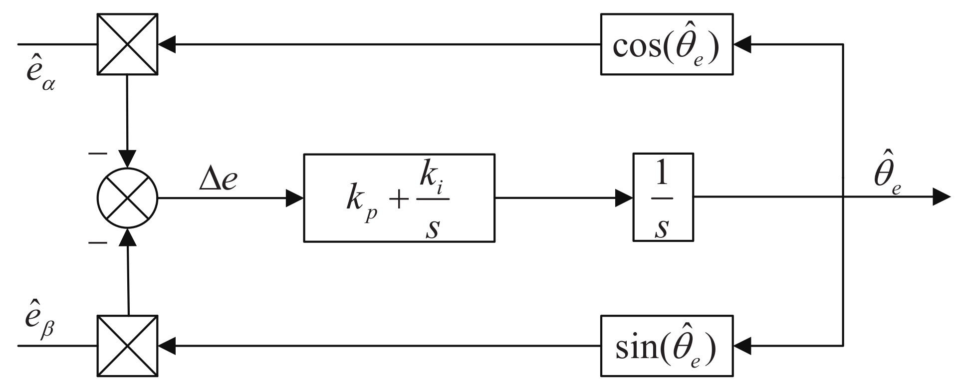
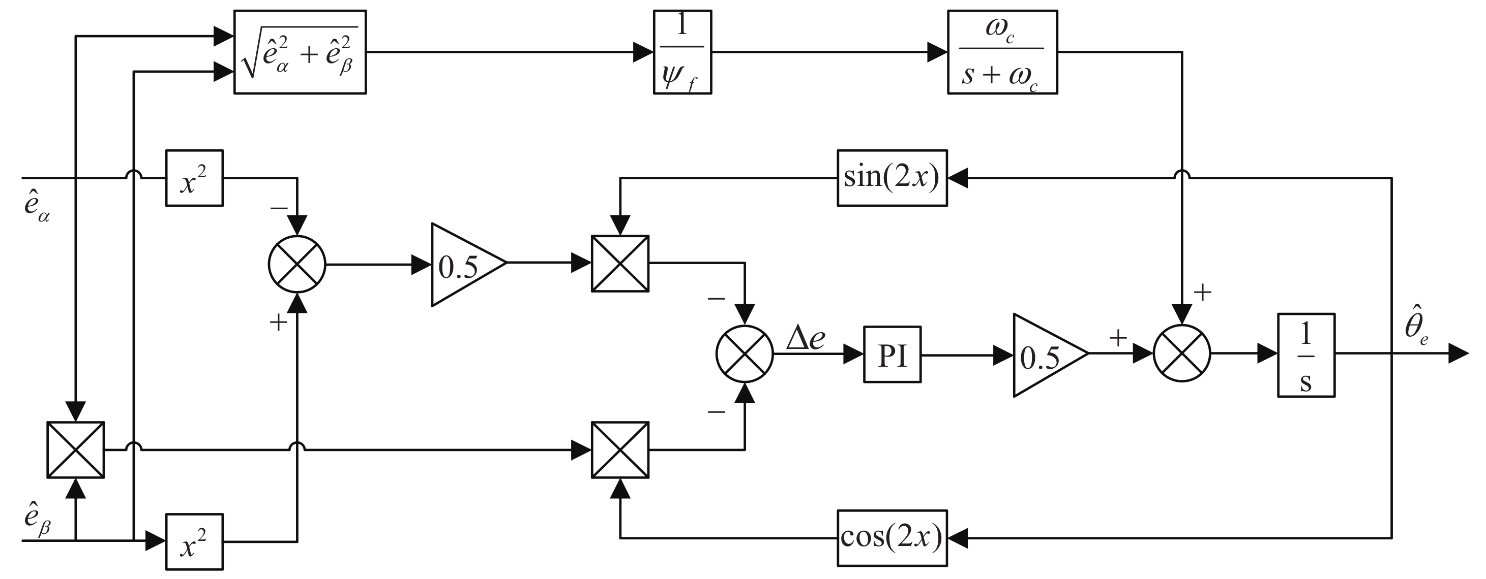
4. Rotor Position and Speed Extraction

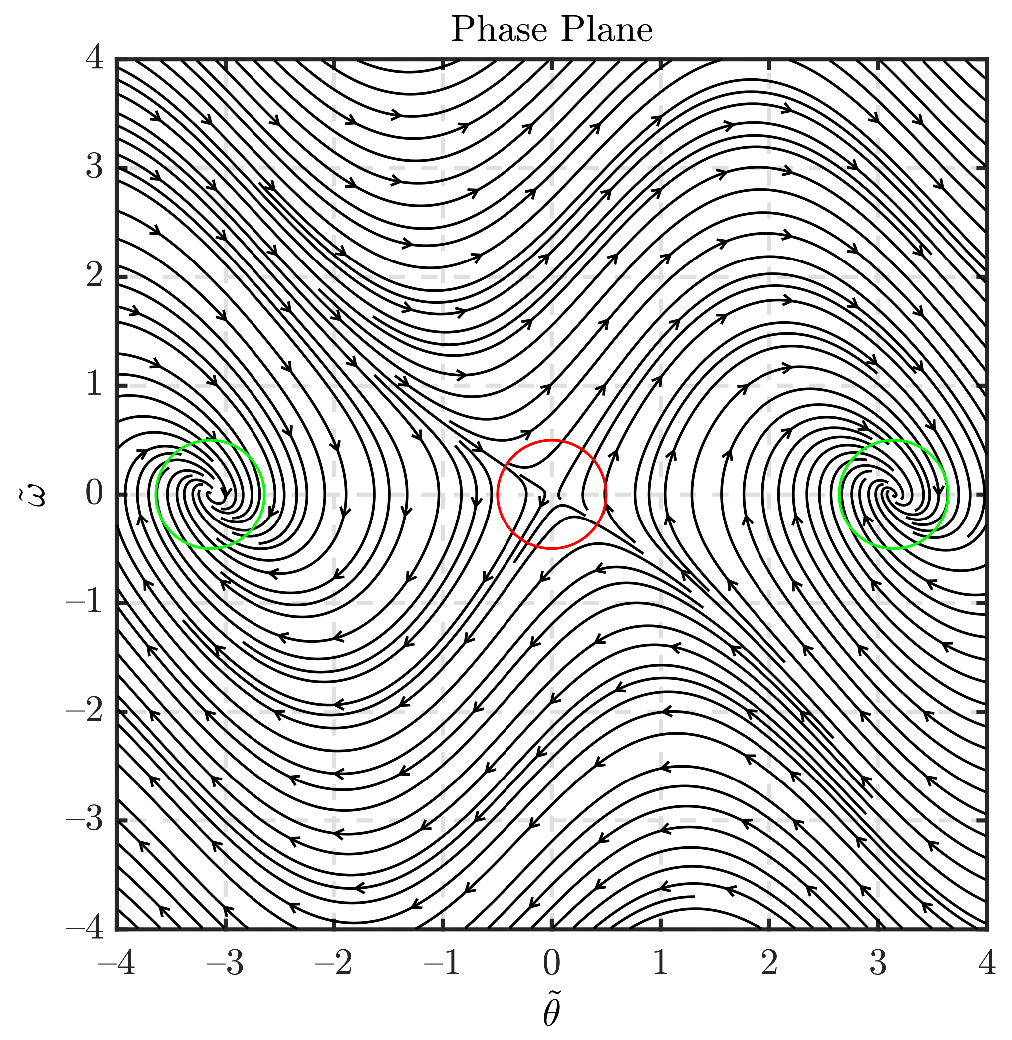
4.1. Traditional PLL Analysis

The PLL is significantly more stable than the arctangent function for extracting rotor position information from the back-EMF, whose structure and equivalent model are depicted in Figure 3 and Figure 4, respectively. However, in the conventional PLL, once the controller parameters are determined, the motor only runs in a single direction and the position information cannot be estimated accurately if the parameters are not modified when the motor reverses in the other direction. In addition, when the motor is accelerating or decelerating, the estimation error is significant. In Figure 3 and Figure 4, ${\theta }_e$, ${\widehat{\theta }}_e$ mean the rotor electrical angle and the estimated value of the electrical angle, respectively, $\mathrm{\Delta }e$ indicates the electrical angle estimation error, and $k_p$, $k_i$ denote the proportional coefficient and integral coefficient of the PI in the PLL, respectively.

When the motor is rotating in the forward direction, the conventional PLL dynamics equation is as follows.

$$\begin{array}{c}\hfill \left\{\begin{array}{cc}\hfill & \frac{d\tilde{\theta }}{dt}=\tilde{\omega }\hfill \\ \hfill & \frac{d\tilde{\omega }}{dt}=-k_{p}cos\left(\tilde{\theta }\right)\tilde{\omega }-k_{I}sin\left(\tilde{\theta }\right)\hfill \end{array}\right.\end{array}$$

(25)

where $\tilde{\omega }=\omega -\widehat{\omega }$ is the electrical angular velocity estimation error and $k_p$, $k_I$ are positive. The phase plane of the system is shown in Figure 5, where $(\pm \pi ,0)$ is the saddle point, and $(0,0)$ is the stable focus. The trajectory in the phase plane of the system would converge to the origin, i.e., the position and velocity estimation errors would converge to zero, and the system would be able to precisely estimate the rotor position.

When the motor is reversed, the back-EMF of the motor would change from Equation (3) to Equation (20).

$$\begin{array}{c}\hfill \left\{\begin{array}{cc}\hfill & e_{\alpha }={\psi }_f{\omega }_{e}sin\left({\theta }_e\right)\hfill \\ \hfill & e_{\beta }=-{\psi }_f{\omega }_{e}cos\left({\theta }_e\right)\hfill \end{array}\right.\end{array}$$

(26)

At this stage, the dynamics equation of a conventional PLL is as follows:

$$\begin{array}{c}\hfill \left\{\begin{array}{cc}\hfill & \frac{d\tilde{\theta }}{dt}=\tilde{\omega }\hfill \\ \hfill & \frac{d\tilde{\omega }}{dt}=k_{p}cos\left(\tilde{\theta }\right)\tilde{\omega }+k_{I}sin\left(\tilde{\theta }\right)\hfill \end{array}\right.\end{array}$$

(27)

The phase plane diagram of the system is shown in Figure 6, where $(\pm \pi ,0)$ is the stable focus, and $(0,0)$ is the saddle point. Therefore, the system is stable at $(\pm \pi ,0)$. In such a case, the PLL would not converge the rotor position error to zero, but rather generate a $\pi$ deviation. When the motor is reversed, the conventional PLL would be unable to reliably detect the rotor position.

According to Figure 4, the error closed-loop transfer function can be obtained as

$$\begin{array}{c}\hfill {\mathrm{\Phi }}_{ess0}\left(s\right)=\frac{s^2}{s^2+k_{p}s+k_I}\end{array}$$

(28)

When the motor is accelerated or decelerated, the input is acceleration equivalent to the angle. Assuming that the aforementioned transfer function is provided with a unit acceleration input, the steady-state error can be calculated as follows:

$$\begin{array}{c}\hfill \begin{array}{cc}\hfill e_{ss0}& =\underset{s\to 0}{lim}s·{\mathrm{\Phi }}_{ess0}\left(s\right)·\frac{1}{s^3}\hfill \\ \hfill & =\underset{s\to 0}{lim}\frac{1}{s^2+k_{p}s+k_I}\hfill \\ \hfill & =\frac{1}{K_I}\hfill \end{array}\end{array}$$

(29)

It is known that the steady-state error of the system is not 0 at this time, and the steady-state error of the system would be reduced when increasing the integral coefficient $k_I$. However, increasing the integral coefficient $k_I$ may cause the stability of the system degradation. Therefore, under the traditional PLL, the rotor position error cannot converge to 0.

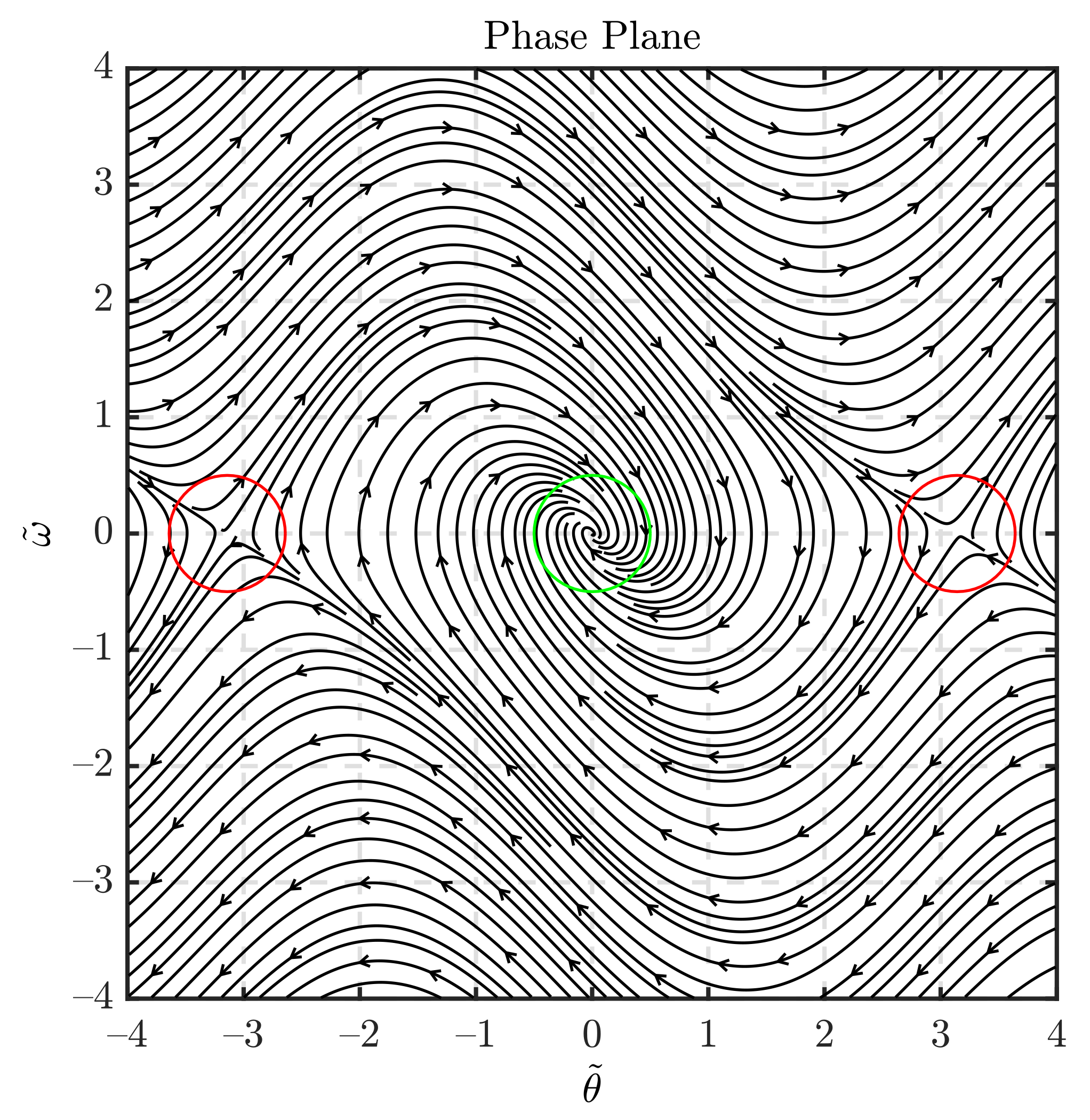
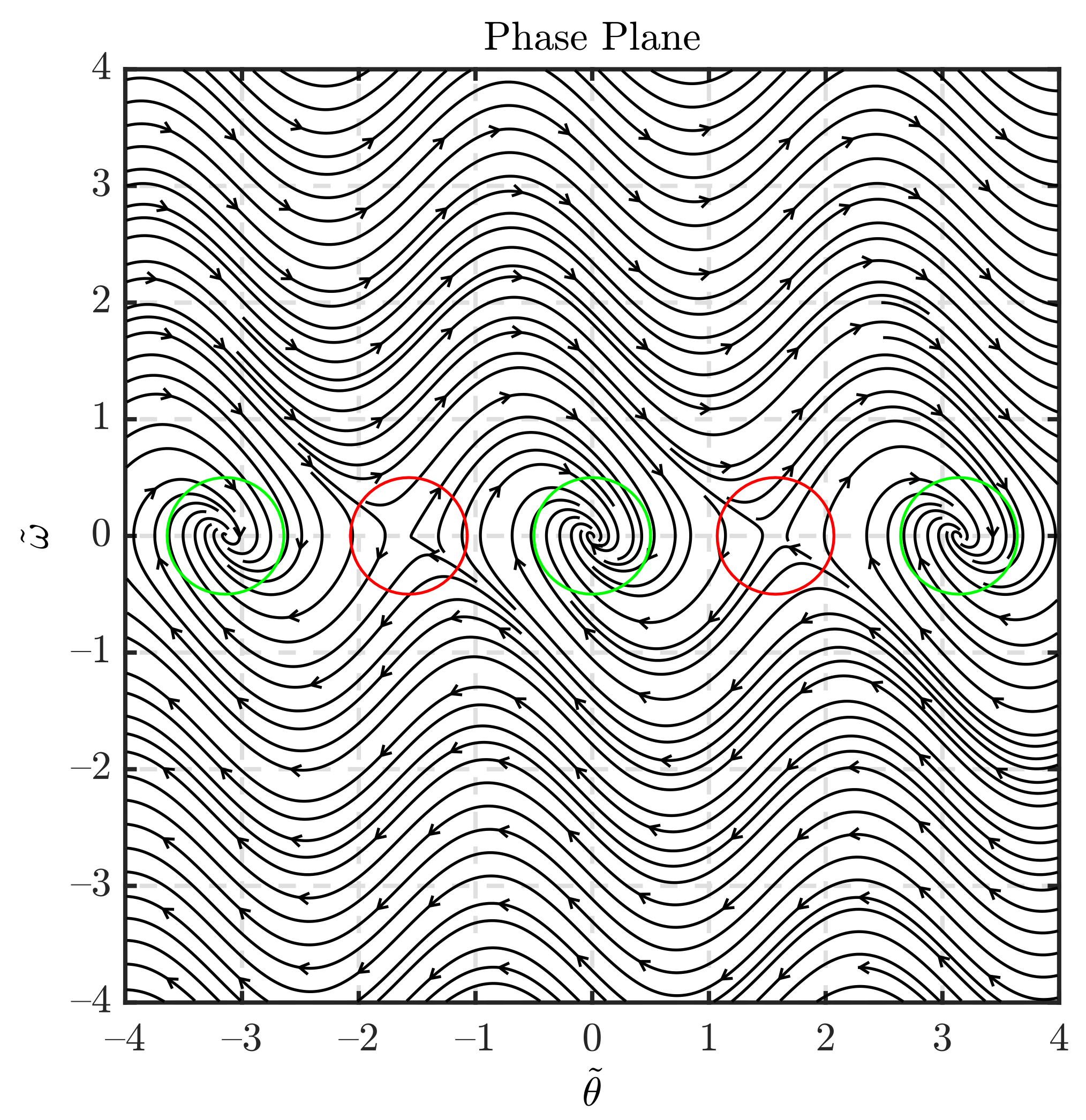
4.2. Improved PLL Analysis

Based on the deficiencies of the traditional PLL outlined in the previous section, this section will provide an improved PLL and demonstrate its stability. The structure diagram of the improved PLL is shown in Figure 7. The relationship between $\mathrm{\Delta }e$ and ${\theta }_e$, ${\widehat{\theta }}_e$ is as follows.

$$\begin{array}{c}\hfill \begin{array}{cc}\hfill \mathrm{\Delta }e& =-[\frac{1}{2}(e_{\alpha }^2+e_{\beta }^2)sin\left(2{\widehat{\theta }}_e\right)]-[e_{\alpha }{e}_{\beta }cos\left(2{\widehat{\theta }}_e\right)]\hfill \\ \hfill & =-\frac{1}{2}{\psi }_f^2{\omega }_e^{2}cos\left(2{\theta }_e\right)sin\left(2{\widehat{\theta }}_e\right)+\frac{1}{2}{\psi }_f^2{\omega }_e^{2}sin\left(2{\theta }_e\right)cos\left(2{\widehat{\theta }}_e\right)\hfill \\ \hfill & =\frac{1}{2}{\psi }_f^2{\omega }_e^{2}sin2({\theta }_e-{\widehat{\theta }}_e)\propto sin\left(2{\tilde{\theta }}_e\right)\hfill \end{array}\end{array}$$

(30)

When the PLL is steadily tracking the rotor position, ${\tilde{\theta }}_e\to 0$, ${\widehat{\theta }}_e\approx {\theta }_e$.

Combining Equations (3), (26), and (30), when the improved PLL is used, its dynamic equation is as follows whether the motor is in forward or reverse rotation.

$$\begin{array}{c}\hfill \left\{\begin{array}{cc}\hfill & \frac{d\tilde{\theta }}{dt}=\tilde{\omega }\hfill \\ \hfill & \frac{d\tilde{\omega }}{dt}=\frac{1}{2}[-k_{p}cos\left(2\tilde{\theta }\right)·2\tilde{\omega }-k_{I}sin\left(2\tilde{\theta }\right)]\hfill \end{array}\right.\end{array}$$

(31)

The phase plane diagram of the system is shown in Figure 8, where $(\pm \pi ,0),(0,0),$$(\pm 0.5\pi ,0)$ are the five balance points of the system, $(\pm 0.5\pi ,0)$ are the saddle points, and $(\pm \pi ,0),(0,0)$ are the stable focus. The trajectory in the phase plane of the system would approach the origin. That is, the position and speed estimation errors would converge to zero. At this time, ${\widehat{\theta }}_e\approx {\theta }_e$, the system can accurately estimate the position and speed of the rotor. The improved PLL open-loop transfer function is

$$\begin{array}{c}\hfill G_1\left(s\right)=\frac{(k_p+{\omega }_c)s^2+(k_I+k_p{\omega }_c)s+k_I{\omega }_c}{s^2(s+{\omega }_c)}\end{array}$$

(32)

where ${\omega }_c$ is the cut-off frequency of the LPF in the feedforward channel. By Equation (26), the error closed-loop transfer function of the rotor position can be obtained as

$$\begin{array}{c}\hfill {\mathrm{\Phi }}_{ess1}\left(s\right)=\frac{s^3}{(s+{\omega }_c)(s^2+k_{p}s+k_I)}\end{array}$$

(33)

When the motor is accelerated or decelerated, the input is the acceleration equivalent to the angle. Assuming that a unit acceleration input is added to the above transfer function, according to the final value theorem, the steady-state error can be obtained as

$$\begin{array}{c}\hfill \begin{array}{cc}\hfill e_{ss1}& =\underset{s\to 0}{lim}s{\mathrm{\Phi }}_{ss1}\left(s\right)\frac{1}{s^3}\hfill \\ \hfill & =\underset{s\to 0}{lim}s·\frac{s^3}{(s+{\omega }_c)(s^2+k_{p}s+k_I)}·\frac{1}{s^3}\hfill \\ \hfill & =0\hfill \end{array}\end{array}$$

(34)

The improved PLL can reduce the rotor position error to 0 caused by the PLL when the motor is accelerating and decelerating. Therefore, the improved PLL can extract the position information of the rotor more accurately than the traditional PLL.

To sum up, there are two main improvements of the improved PLL:

(1)

Improve the inability of the conventional PLL to reliably extract position information during motor reversal;

(2)

During motor acceleration and deceleration, the conventional PLL’s error problem has been resolved.

Therefore, the structure of the PMSM position sensorless control system based on SMO is shown in Figure 9.

5. Simulation Verification

To verify the feasibility of the proposed PMSM sensorless control algorithm based on hyperbolic tangent SMO and improved PLL, a simulation model is built in Matlab/Simulink according to Figure 9, and the simulation parameters are shown in

Table 1. Main parameters of PMSM.

Parameter	Value
number of pole pairs p	4
stator resistance $R_s$	2.875 $\mathrm{\Omega }$
stator inductor $L_s$	8.5 $\mathrm{mH}$
rotational inertia J	0.001 $\mathrm{kg}·{\mathrm{m}}^2$
permanent magnet flux ${\psi }_f$	0.175 $\mathrm{Wb}$
DC voltage $U_{dc}$	311 $\mathrm{V}$

.

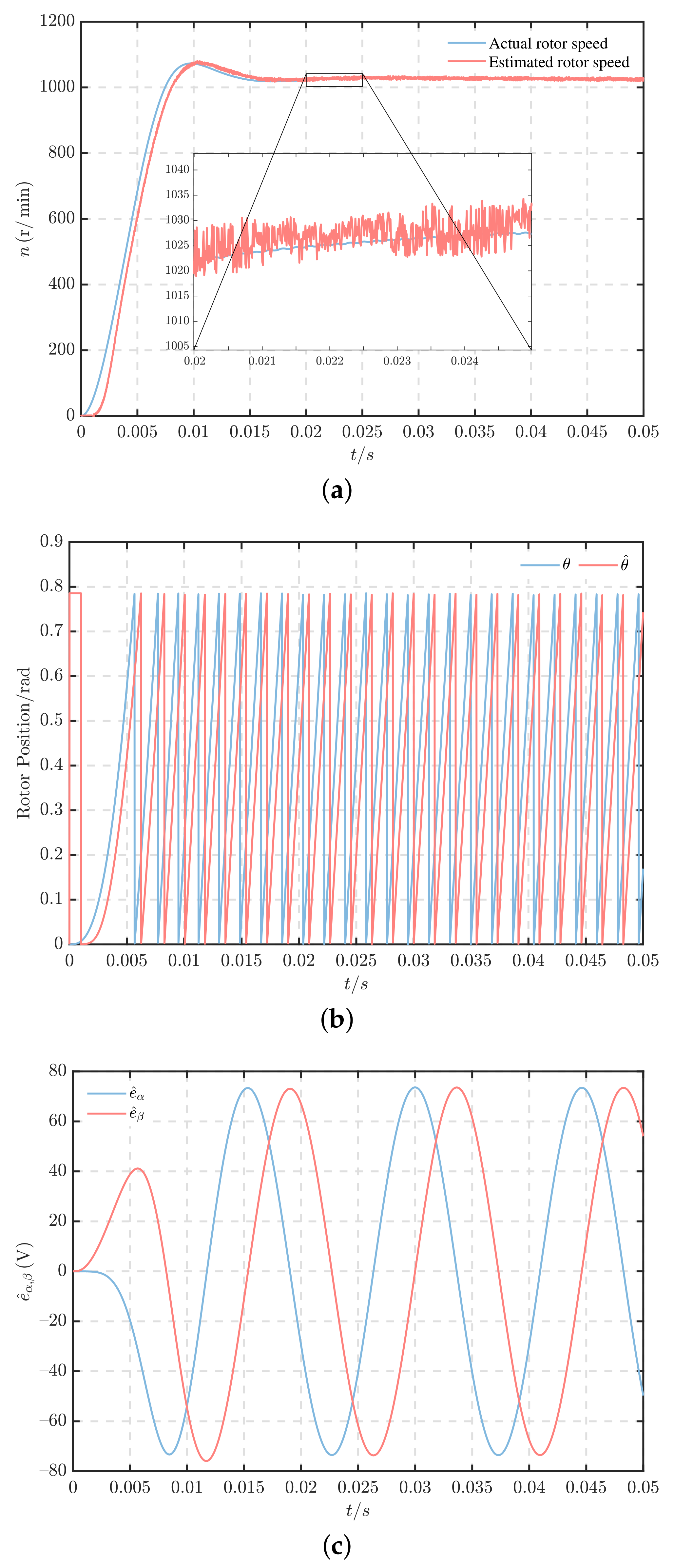
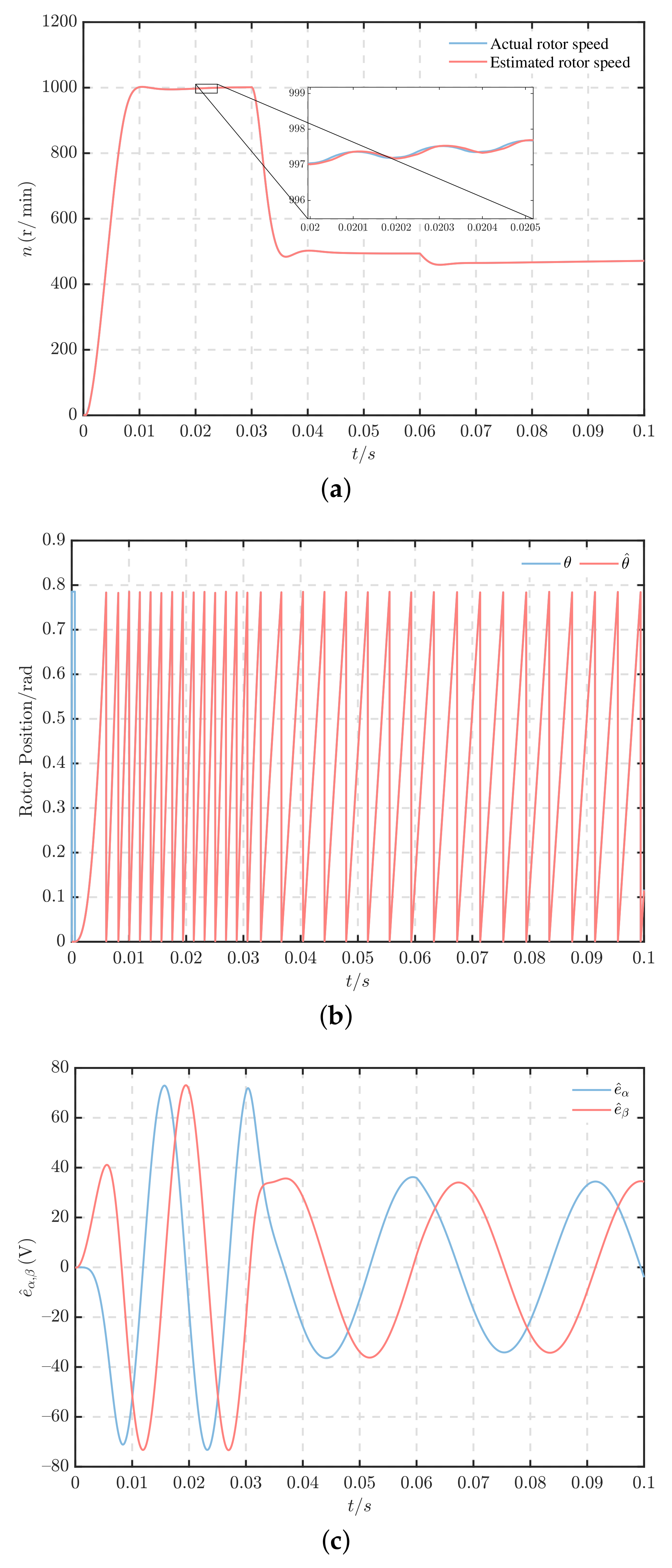
5.1. Steady-State Performance

This experiment focuses on examining the steady-state performance differences between conventional SMO combined with conventional PLL and improved SMO combined with feedforward PLL.

Set the parameters of the improved SMO to $h=0.01$, $\lambda =100$, $\mu =300$, $m=100$. The parameter of traditional SMO is set to $\lambda =1000$, ${\omega }_c=2000$. The parameters of both feedforward PLL and conventional PLL are set to $k_p=100$, $k_I$ = 10,000.

When the motor is unloaded and its speed is set to 1000 r/min, the steady-state performance of the motor under each algorithm is compared. From Figure 10a and Figure 11a, it can be observed that both the conventional algorithm and the improved algorithm can keep the motor running steadily, with the conventional algorithm having a speed fluctuation range of ±5 r/min and the improved algorithm having a speed fluctuation range of ±0.1 r/min. Therefore, the improved SMO may effectively mitigate the speed chattering issue. The peak rotor position estimation error is 0.255 rad and the steady-state error is 0.212 rad for the conventional algorithm, whereas the peak rotor position estimation error is 0.0043 rad and the steady-state error is 0.0042 rad for the improved algorithm (Figure 10b, Figure 11b and Figure 12). Consequently, the improved feedforward PLL provides superior position tracking performance.

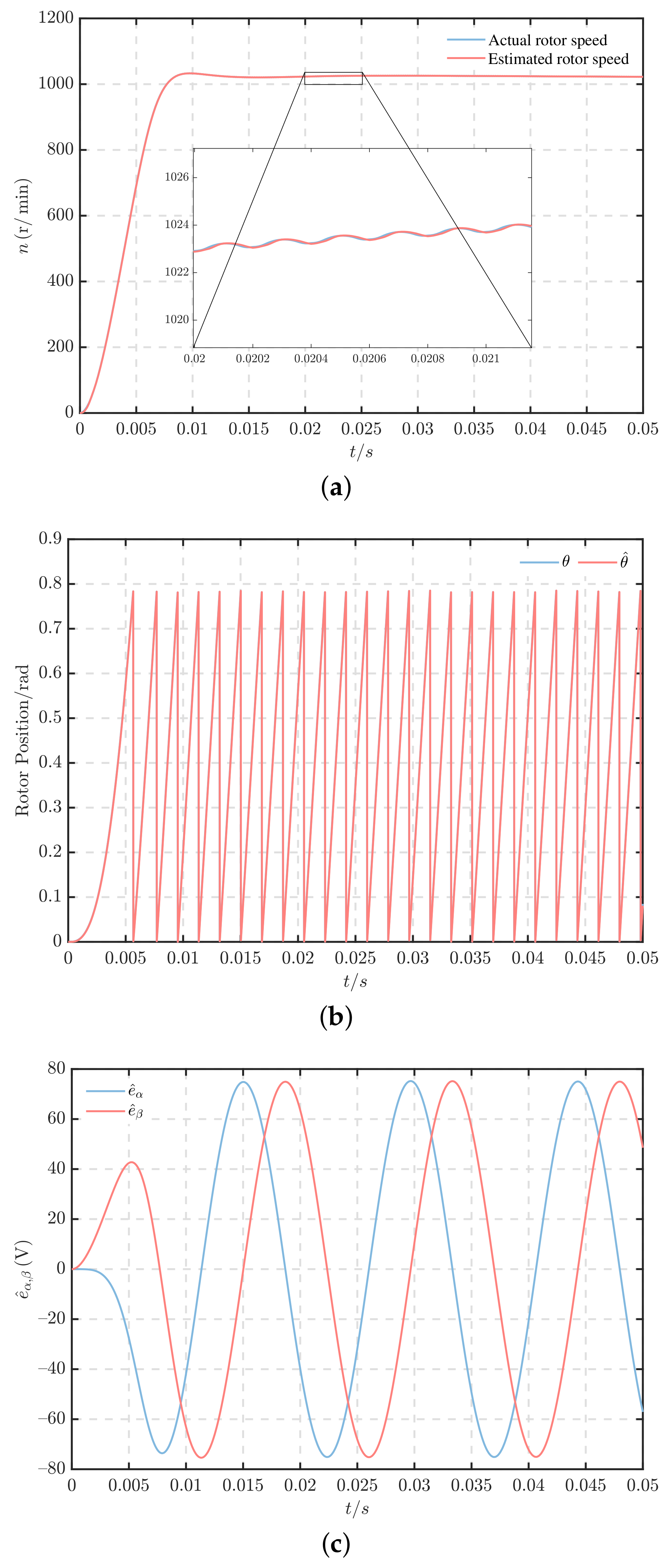
5.2. Dynamic Performance

This experiment focuses on comparing the dynamic performance differences between the conventional SMO combined with the conventional PLL algorithm and the improved SMO combined with feedforward PLL when acceleration, deceleration, and sudden load addition are encountered.

First, set the initial load of the motor to 2 N·m and the initial given speed to 1000 r/min. When the motor runs to 0.03 s, set the given speed to 500 r/min to decelerate the motor. Add a sudden 4 N·m load to the motor while it has been running for 0.06 s. From Figure 13a and Figure 14a, it can be seen that the conventional algorithm has a speed fluctuation range of ±5 r/min in the initial state and an overshoot of 4%. The improved algorithm has a speed fluctuation range of ±0.1 r/min and an overshoot of 0.3% in the initial state. In the case of motor deceleration, the adjustment time of the conventional algorithm is 15 ms, while the adjustment time of the improved algorithm is 6 ms. In the case of load surge, the speed drop of the conventional algorithm is 50 r/min and the adjustment time is 10 ms, while the speed drop of the improved algorithm is 40 r/min and the adjustment time is 6 ms. Figure 13b, Figure 14b and Figure 15 reveal that the traditional algorithm rotor position estimation error peaks at 0.25 rad, while the improved algorithm rotor position estimation error peaks at 0.0043 rad. After motor deceleration and sudden load application, the conventional algorithm rotor position estimation error is 0.1 rad, but the improved algorithm rotor position estimation error can quickly converge to 0.002 rad. Therefore, the improved SMO can make the motor maintain good stability and low chattering during dynamic operation. The improved PLL can keep the rotor position estimation error low during acceleration and deceleration, so that the rotor position information can be extracted more accurately.

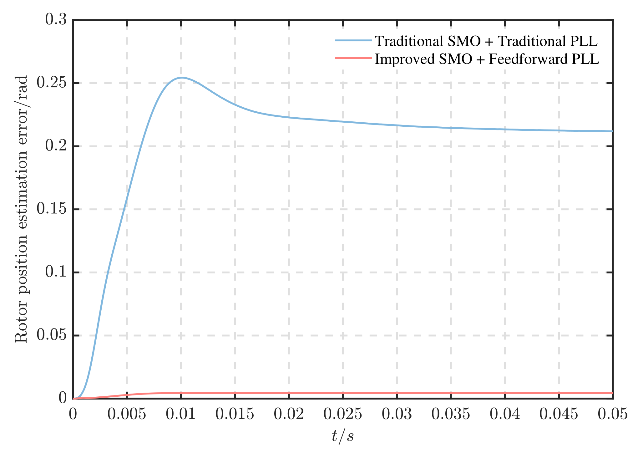
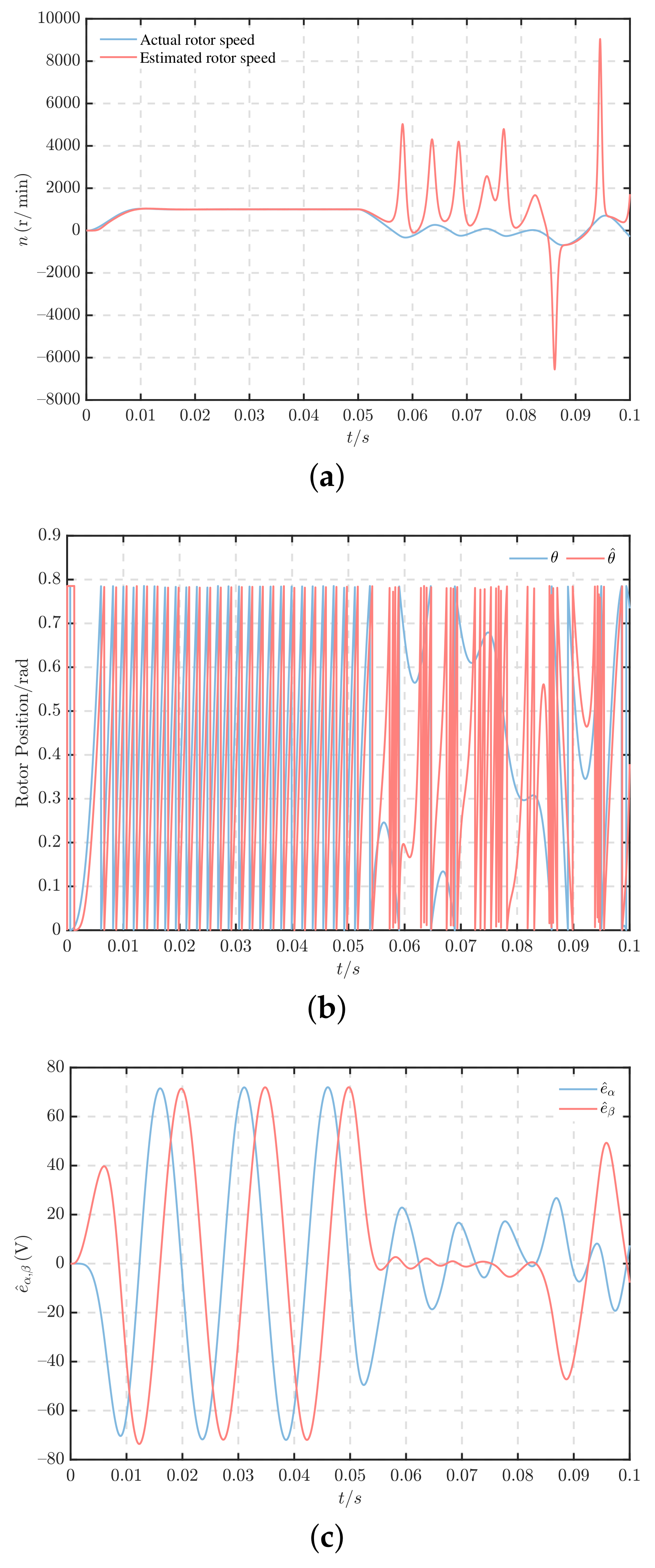
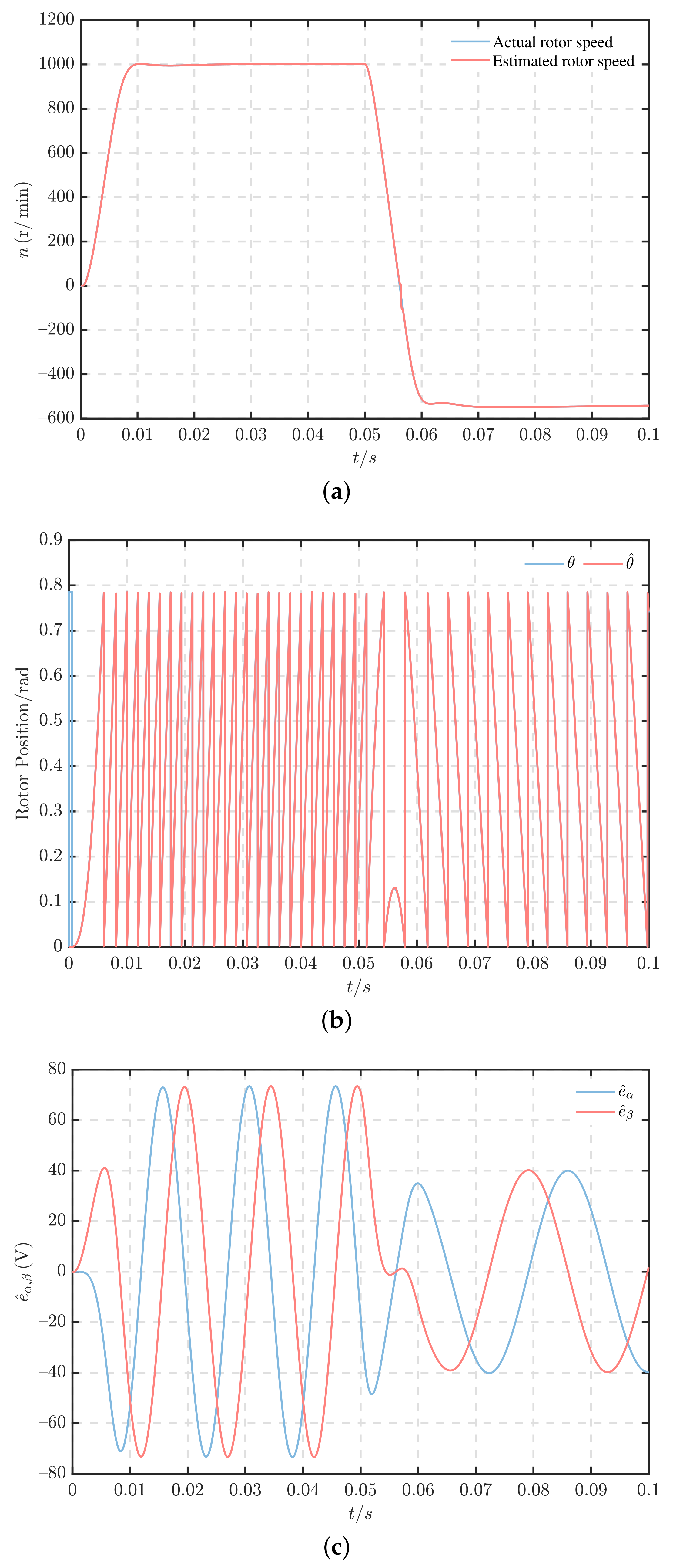
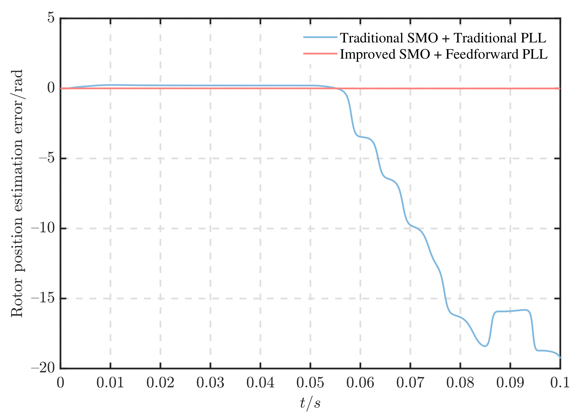
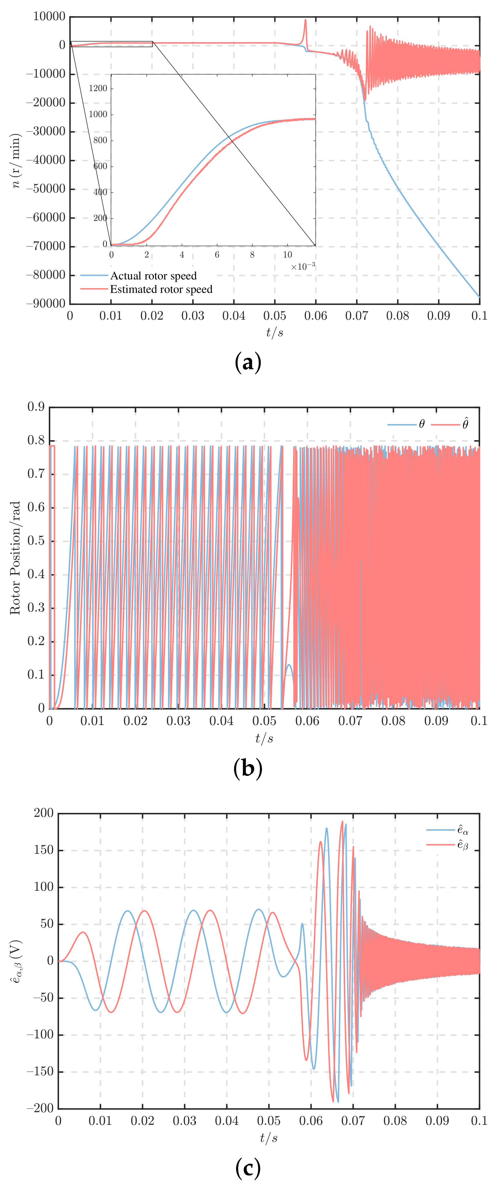
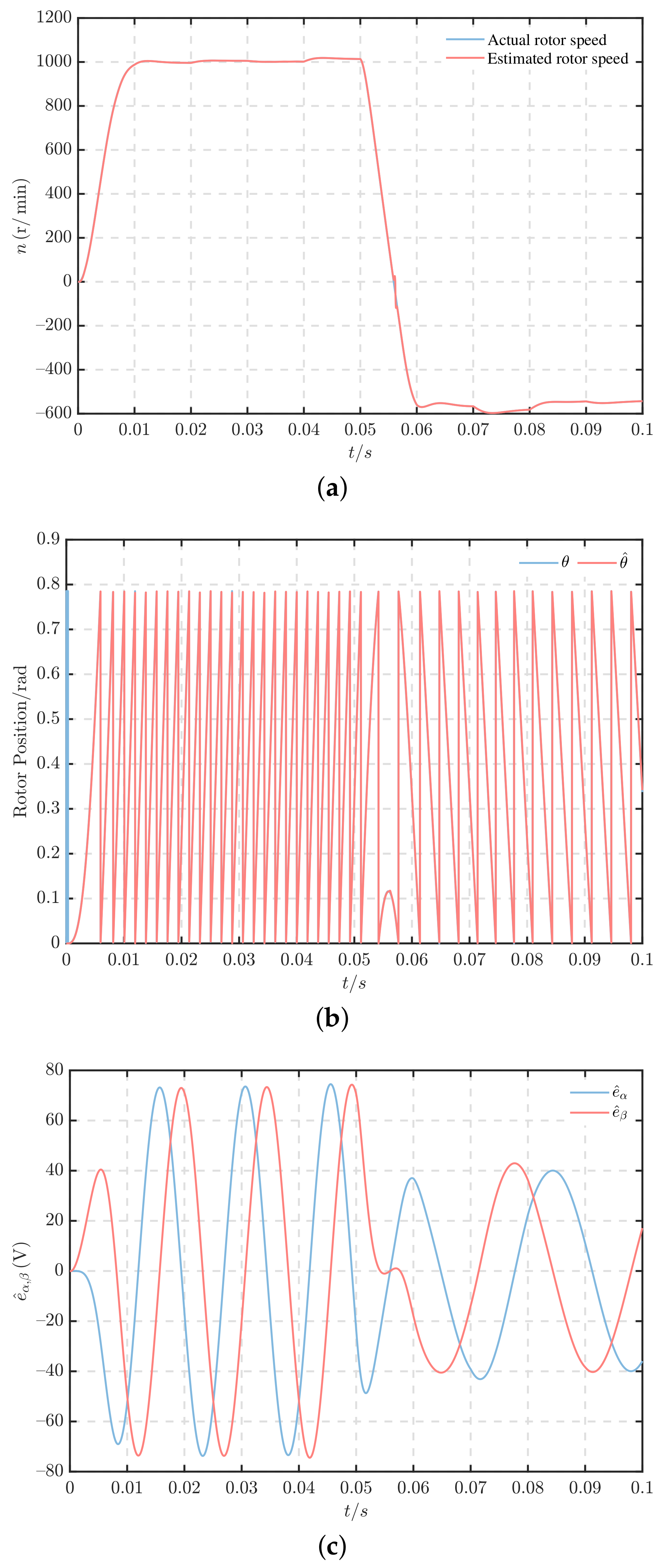
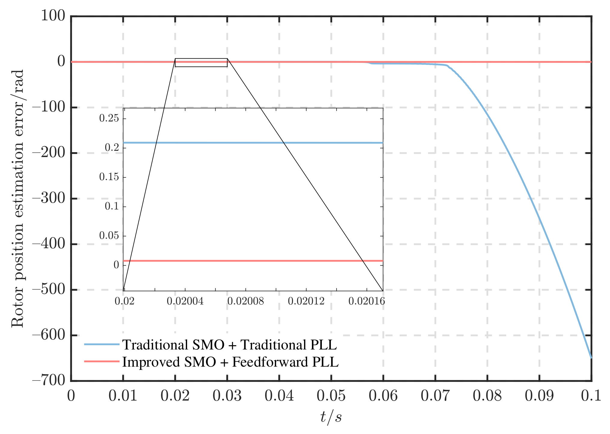
5.3. Forward and Reverse

The main purpose of this experiment is to verify that the improved feedforward PLL can accurately extract rotor position information in both forward and reverse motor rotation.

The motor load is initially set to 2 N·m and the initial given speed is set to 1000 r/min. To simulate the motor reverse, the given speed is adjusted to −500 r/min for 0.05 s. From Figure 16, Figure 17 and Figure 18, it is evident that the improved PLL can accurately identify the rotor position information when the motor is reversed and maintain stable motor operation, whereas the conventional PLL cannot extract the rotor position information correctly when the motor is reversed, resulting in unstable motor operation. Consequently, the improved PLL can better maintain the stability of the ship motor control system in the face of the frequent forward and reverse rotation requirements of ship motors.

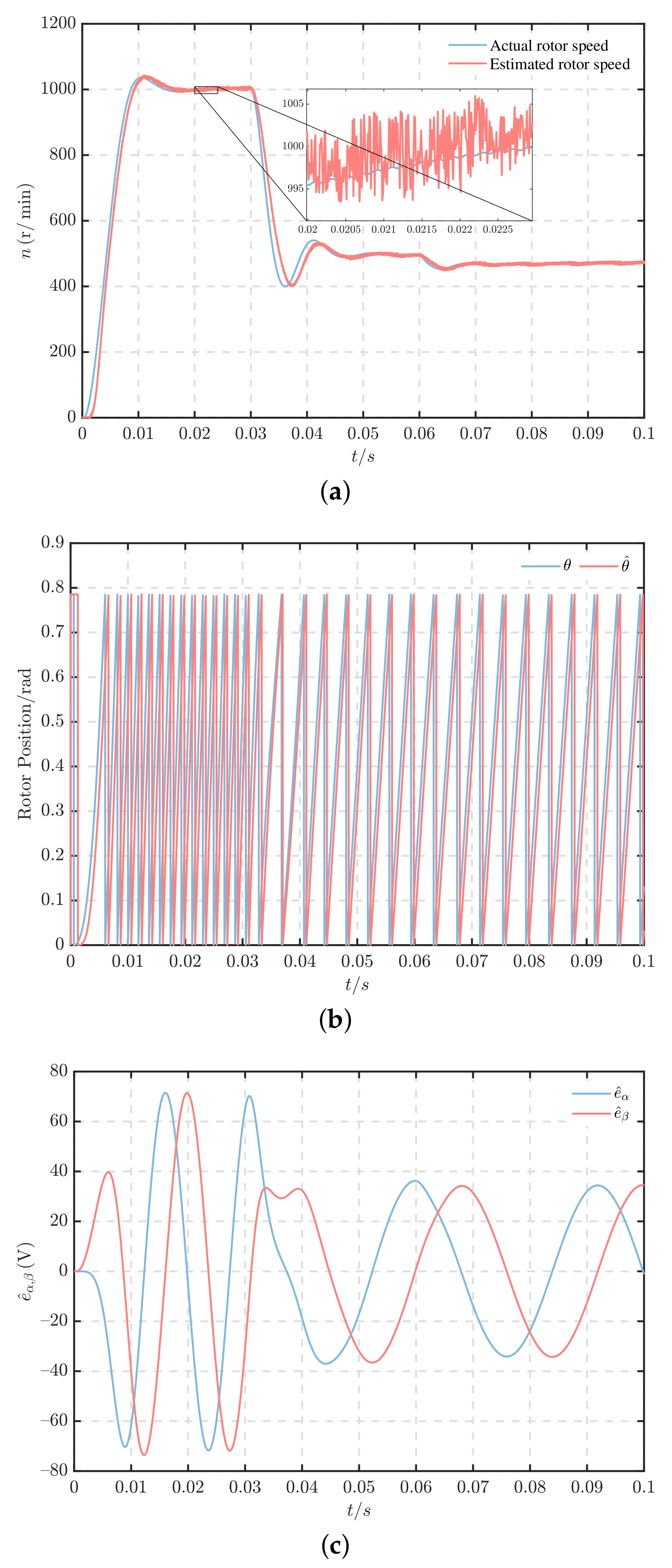
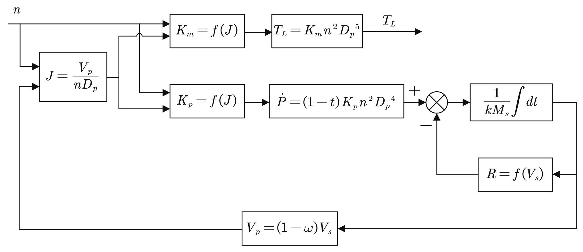
5.4. Performance under Ship Propeller Load

The motor position sensorless control algorithm proposed in this paper is mainly applied to electric propulsion ships, so it is necessary to verify the effectiveness of the algorithm under the ship propeller load. In addition, to verify the robustness of the algorithm in this paper, a random noise is applied to the load torque to simulate the disturbance of wind and waves in the ocean.

According to Ref. [30], the dynamic load model of the ship propeller is shown in Figure 19. Based on the propeller load model and the model parameter values shown in

Table 2. Main parameters of PMSM.

Parameter	Value
Propeller diameter $D_p$/m	0.1
Hull mass $M_s$/kg	100
Water attachment coefficient k	1.1
Wake coefficient $\omega$	0.12285
Thrust derating coefficient t	0.146

, the simulation model is established. The relationship between the motor speed and its load when the ship is sailing can be obtained. The effectiveness of the improved SMO and improved feedforward PLL is proposed in this paper for the dynamic environment of ship navigation. In Figure 19, n is the propeller speed of the motor, unit is rad/s, $T_L$ is the propeller torque, unit is N·m, J is the advance ratio of the propeller, $D_p$ is the diameter of the propeller, unit is m, P is the thrust generated by the rotation of the propeller, unit is N, $M_s$ is the mass of the ship, unit is kg, R is the resistance of the ship, unit is N, $V_s$ is the speed of the ship, unit is m/s, $V_p$ is the propeller advance speed, unit is m/s, $\omega$ is the wake coefficient, t is the thrust derating coefficient, k is the water attachment coefficient, $K_p$ is the dimensionless coefficient of propeller thrust, and $K_m$ is the dimensionless coefficient of drag torque.

$$\begin{array}{c}\hfill \left\{\begin{array}{cc}\hfill & K_p=0.38955-0.27115J-0.10256J^2\hfill \\ \hfill & K_m=0.049543-0.021832J-0.02079J^2\hfill \end{array}\right.\end{array}$$

(35)

The PMSM load perturbation was set to propeller load while introducing random perturbations. The initial speed was set to 1000 r/min, and after the motor ran for 0.05 s, the speed was set to −500 r/min to simulate motor reversal. As shown in Figure 20a, in the presence of random noise, the conventional algorithm ensures system stability in forward rotation, with a speed fluctuation range of ±50 r/min. However, in reverse rotation, the conventional algorithm causes the system to become unstable. From Figure 21a, it can be observed that the improved algorithm ensures system stability in both forward and reverse rotation, with a speed fluctuation range of ±20 r/min. The improved algorithm effectively reduces speed fluctuation under disturbance while ensuring stable forward and reverse rotation. From Figure 22, the maximum rotor position estimation error of the conventional algorithm is 0.231 rad, whereas the maximum rotor position estimation error of the improved algorithm is only 0.008 rad. Thus, the improved algorithm can significantly reduce the rotor estimation error and improve the position estimation accuracy. In conclusion, the algorithm exhibits excellent anti-interference performance and can adapt to complex marine environments.

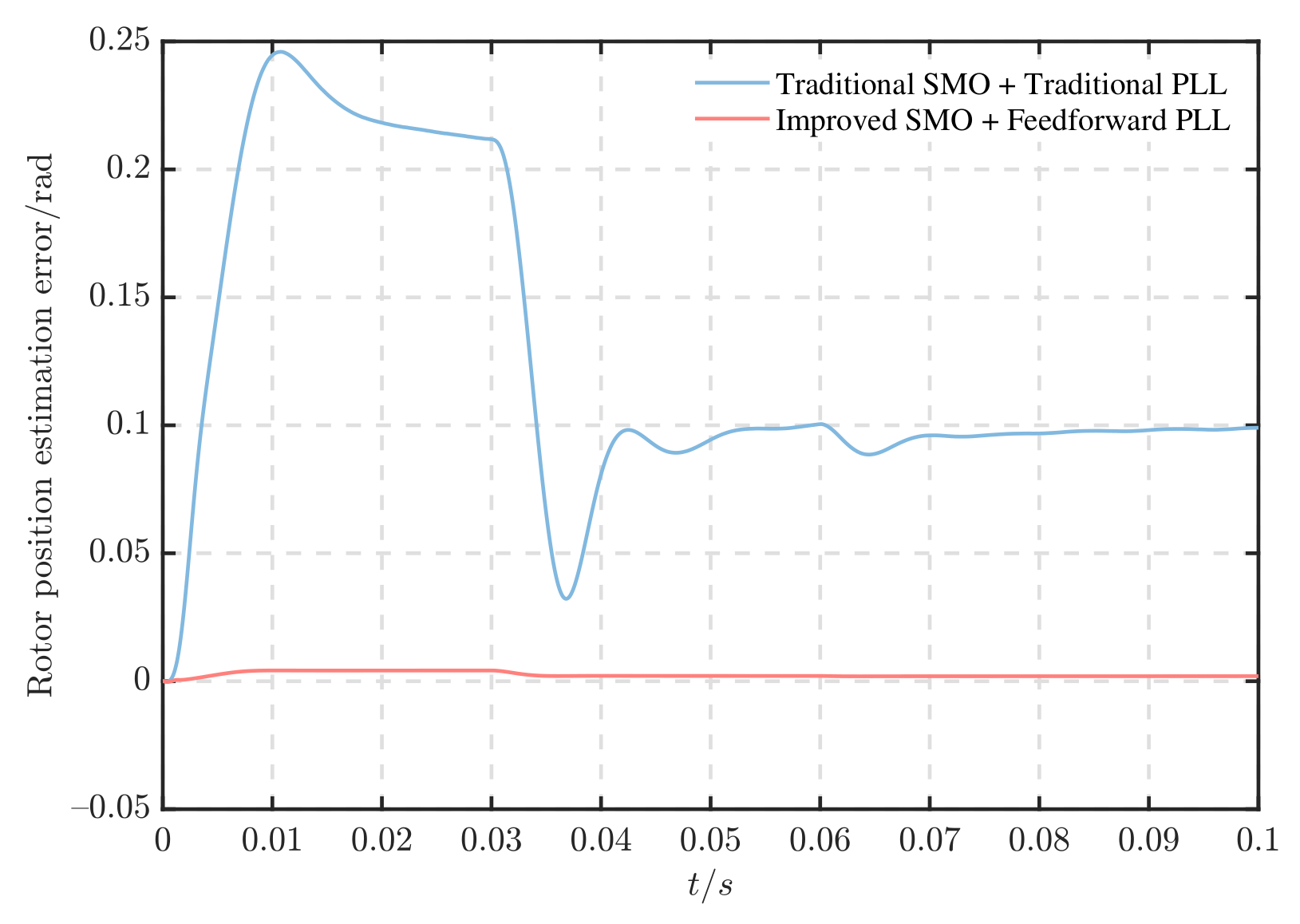
6. Conclusions and Outlook

This paper presents an improved algorithm for position sensorless control of PMSM, which is specifically designed for electric propulsion ships equipped with shaftless RDTs. The primary goal of this algorithm is to enhance the reliability of the motor control system. The algorithm utilizes continuous hyperbolic tangent functions instead of discontinuous symbolic functions to address the chattering problem of SMO. An observer based on the back-EMF model is constructed to extract the back-EMF accurately and minimize speed fluctuations, which effectively reduces the sliding mode gain of the SMO and eliminates the phase delay caused by LPF. Furthermore, the improved feed-forward PLL is introduced to minimize rotor position estimation errors during acceleration and deceleration, as well as to achieve accurate extraction of rotor position information during motor reversal, outperforming the conventional PLL.

To verify the reliability of the algorithm in a complex marine environment, a ship propeller load model and random load are introduced. The simulation results demonstrate the superiority of the improved algorithm over the conventional algorithm consisting of a conventional SMO and a conventional PLL. The improved algorithm achieves smaller speed fluctuations in the face of disturbances, which is beneficial for the stable operation of the ship. It also shows good performance in bi-directional rotation of the motor and can stably track the rotor position, which is important for the frequent forward and reverse rotation of the ship’s RDT motor.

Our future work will validate the algorithm in a real motor and apply it to a real ship, which will greatly contribute to the realization of green and sustainable ship technology.

References

1. Bai, H.; Yu, B. Position estimation of fault-tolerant permanent magnet motor in electric power propulsion ship system. IEEJ Trans. Electr. Electron. Eng. 2022, 17, 890–898. [Google Scholar] [CrossRef]
2. Du, J.; Li, J.; Lewis, F.L. Distributed 3D Time-Varying Formation Control of Underactuated AUVs with Communication Delays Based on Data-Driven State Predictor. IEEE Trans. Ind. Inform. 2022, 1–9, early access. [Google Scholar] [CrossRef]
3. Qin, J.; Du, J. Robust adaptive asymptotic trajectory tracking control for underactuated surface vessels subject to unknown dynamics and input saturation. J. Mar. Sci. Technol. 2022, 27, 307–319. [Google Scholar] [CrossRef]
4. Qin, J.; Du, J.; Li, J. Adaptive finite-time trajectory tracking event-triggered control scheme for underactuated surface vessels subject to input saturation. IEEE Trans. Intell. Transp. Syst. 2023, 1–11, early access. [Google Scholar] [CrossRef]
5. Chen, X.; Wang, Z.; Hua, Q.; Shang, W.; Luo, Q.; Yu, K. AI-Empowered Speed Extraction via Port-like Videos for Vehicular Trajectory Analysis. IEEE Trans. Intell. Transp. Syst. 2023, 1–12, early access. [Google Scholar] [CrossRef]
6. Qin, J.; Du, J. Minimum-learning-parameter-based adaptive finite-time trajectory tracking event-triggered control for underactuated surface vessels with parametric uncertainties. Ocean Eng. 2023, 271, 113634. [Google Scholar] [CrossRef]
7. Chen, X.; Liu, S.; Liu, W.; Wu, H.; Han, B.; Zhao, J. Quantifying Arctic oil spilling event risk by integrating analytic network process and fuzzy comprehensive evaluation model. Ocean Coast. Manag. 2022, 228, 106326. [Google Scholar] [CrossRef]
8. Bai, H.; Yu, B.; Ouyang, W.; Yan, X.; Zhu, J. HF-based sensorless control of a FTPMM in ship shaftless rim-driven thruster system. IEEE Trans. Intell. Transp. Syst. 2022, 23, 16867–16877. [Google Scholar] [CrossRef]
9. Yan, X.; Liang, X.; Ouyang, W.; Liu, Z.; Liu, B.; Lan, J. A review of progress and applications of ship shaft-less rim-driven thrusters. Ocean Eng. 2017, 144, 142–156. [Google Scholar] [CrossRef]
10. Sulligoi, G.; Vicenzutti, A.; Menis, R. All-electric ship design: From electrical propulsion to integrated electrical and electronic power systems. IEEE Trans. Transp. Electrif. 2016, 2, 507–521. [Google Scholar] [CrossRef]
11. Lin, S.; Zhang, W. An adaptive sliding-mode observer with a tangent function-based PLL structure for position sensorless PMSM drives. Int. J. Electr. Power Energy Syst. 2017, 88, 63–74. [Google Scholar] [CrossRef]
12. Bai, H.; Zhu, J.; Qin, J.; Sun, J. Fault-tolerant control for a dual-winding fault-tolerant permanent magnet motor drive based on SVPWM. IET Power Electron. 2017, 10, 509–516. [Google Scholar] [CrossRef]
13. Qiao, Z.W.; Shi, T.N.; Wang, Y.D.; Yan, Y.; Xia, C.L.; He, X.N. New sliding-mode observer for position sensorless control of permanent-magnet synchronous motor. IEEE Trans. Ind. Electron. 2013, 60, 710–719. [Google Scholar] [CrossRef]
14. Yang, Z.; Yan, X.; Ouyang, W.; Bai, H. Sensor lessPMSM Control Algorithm for Rim-Driven Thruster Based on Improved PSO. In Proceedings of the 2021 6th International Conference on Transportation Information and Safety, Wuhan, China, 22–24 October 2021; pp. 285–292. [Google Scholar]
15. Seo, D.; Bak, Y.; Lee, K. An Improved Rotating Restart Method for a Sensorless Permanent Magnet Synchronous Motor Drive System Using Repetitive Zero Voltage Vectors. IEEE Trans. Ind. Electron. 2020, 67, 3496–3504. [Google Scholar] [CrossRef]
16. Wang, G.L.; Valla, M.; Solsona, J. Position Sensorless Permanent Magnet Synchronous Machine Drives-A Review. IEEE Trans. Ind. Electron. 2020, 67, 5830–5842. [Google Scholar] [CrossRef]
17. Zhang, X.G.; Li, Z.X. Sliding-Mode Observer-Based Mechanical Parameter Estimation for Permanent Magnet Synchronous Motor. IEEE Trans. Power Electron. 2016, 31, 5732–5745. [Google Scholar] [CrossRef]
18. Yang, H.; Yang, R.; Hu, W.; Huang, Z.M. FPGA-Based Sensorless Speed Control of PMSM Using Enhanced Performance Controller Based on the Reduced-Order EKF. IEEE J. Emerg. Sel. Top. Power Electron. 2021, 9, 289–301. [Google Scholar] [CrossRef]
19. Abo-Khalil, A.G.; Eltamaly, A.M.; Alsaud, M.S.; Sayed, K.; Alghamdi, A.S. Sensorless control for PMSM using model reference adaptive system. Int. Trans. Electr. Energy Syst. 2021, 31, e12733. [Google Scholar] [CrossRef]
20. Bernard, P.; Praly, L. Estimation of Position and Resistance of a Sensorless PMSM: A Nonlinear Luenberger Approach for a Nonobservable System. IEEE Trans. Autom. Control. 2021, 66, 481–496. [Google Scholar] [CrossRef] [Green Version]
21. Wang, G.L.; Hao, X.F.; Zhao, N.N.; Zhang, G.Q.; Xu, D.G. Current Sensor Fault-Tolerant Control Strategy for Encoderless PMSM Drives Based on Single Sliding Mode Observer. IEEE Trans. Transp. Electrif. 2020, 6, 679–689. [Google Scholar] [CrossRef]
22. Wu, L.G.; Liu, J.X.; Vazquez, S.; Mazumder, S.K. Sliding Mode Control in Power Converters and Drives: A Review. IEEE-CAA J. Autom. Sin. 2022, 9, 392–406. [Google Scholar] [CrossRef]
23. Kang, W.X.; Li, H. Improved sliding mode observer based sensorless control for PMSM. IEICE Electron. Express 2017, 14, 20170934. [Google Scholar] [CrossRef] [Green Version]
24. Wibowo, W.K.; Jeong, S.K. Improved estimation of rotor position for sensorless control of a PMSM based on a sliding mode observer. J. Cent. South Univ. 2016, 23, 1643–1656. [Google Scholar] [CrossRef]
25. Ren, N.N.; Fan, L.; Zhang, Z. Sensorless PMSM Control with Sliding Mode Observer Based on Sigmoid Function. J. Electr. Eng. Technol. 2021, 16, 933–939. [Google Scholar] [CrossRef]
26. Ye, S.C.; Yao, X.X. An Enhanced SMO-Based Permanent-Magnet Synchronous Machine Sensorless Drive Scheme with Current Measurement Error Compensation. IEEE J. Emerg. Sel. Top. Power Electron. 2021, 9, 4407–4419. [Google Scholar] [CrossRef]
27. Yang, Z.B.; Ding, Q.F.; Sun, X.D.; Lu, C.L.; Zhu, H.M. Speed sensorless control of a bearingless induction motor based on sliding mode observer and phase-locked loop. ISA Trans. 2022, 123, 346–356. [Google Scholar] [CrossRef] [PubMed]
28. Gong, C.; Hu, Y.H.; Gao, J.Q.; Wang, Y.G.; Yan, L.M. An Improved Delay-Suppressed Sliding-Mode Observer for Sensorless Vector-Controlled PMSM. IEEE Trans. Ind. Electron. 2020, 67, 5913–5923. [Google Scholar] [CrossRef]
29. Song, X.D.; Fang, J.C.; Han, B.C.; Zheng, S.Q. Adaptive Compensation Method for High-Speed Surface PMSM Sensorless Drives of EMF-Based Position Estimation Error. IEEE Trans. Power Electron. 2016, 31, 1438–1449. [Google Scholar] [CrossRef]
30. Peng, H.; Zhu, X.; Yang, L.; Zhang, G. Robust controller design for marine electric propulsion system over controller area network. Control Eng. Pract. 2020, 101, 104512. [Google Scholar] [CrossRef]
Figure 1. Sign function and hyperbolic tangent function.
Jmse 11 00642 g001
Figure 2. Hyperbolic tangent function for different h.
Jmse 11 00642 g002
Figure 3. Structure of conventional PLL.
Jmse 11 00642 g003
Figure 4. Traditional PLL equivalent model.
Jmse 11 00642 g004
Figure 5. Traditional PLL forward phase plane.
Jmse 11 00642 g005
Figure 6. Traditional PLL reversed phase plane.
Jmse 11 00642 g006
Figure 7. Structure of the improved PLL.
Jmse 11 00642 g007
Figure 8. Improved PLL phase plane.
Jmse 11 00642 g008
Figure 9. Structure of the PMSM position sensorless control system based on SMO.
Jmse 11 00642 g009
Figure 10. Responses of the simulation with conventional SMO combined with conventional PLL (steady-state). (a) Rotor speed. (b) Rotor position. (c) Estimation of the back-EMF.
Jmse 11 00642 g010
Figure 11. Responses of the simulation with improved SMO combined with feedforward PLL (steady-state). (a) Rotor speed. (b) Rotor position. (c) Estimation of the back-EMF.
Jmse 11 00642 g011
Figure 12. Rotor position observation errors (steady-state).
Jmse 11 00642 g012
Figure 13. Responses of simulation with conventional SMO combined with conventional PLL (dynamic). (a) Rotor speed. (b) Rotor position. (c) Estimation of the back-EMF.
Jmse 11 00642 g013
Figure 14. Responses of simulation with improved SMO combined with feedforward PLL (dynamic). (a) Rotor speed. (b) Rotor position. (c) Estimation of the back-EMF.
Jmse 11 00642 g014
Figure 15. Rotor position observation errors (dynamic).
Jmse 11 00642 g015
Figure 16. Responses of the simulation with conventional SMO combined with conventional PLL (forward and reverse). (a) Rotor speed. (b) Rotor position. (c) Estimation of the back-EMF.
Jmse 11 00642 g016
Figure 17. Responses of simulation with the improved SMO combined with feedforward PLL (forward and reverse). (a) Rotor speed. (b) Rotor position. (c) Estimation of the back-EMF.
Jmse 11 00642 g017
Figure 18. Rotor position observation errors (forward and reverse).
Jmse 11 00642 g018
Figure 19. Ship propeller load model.
Jmse 11 00642 g019
Figure 20. Responses of the simulation with conventional SMO combined with conventional PLL (with propeller load). (a) Rotor speed. (b) Rotor position. (c) Estimation of the back-EMF.
Jmse 11 00642 g020
Figure 21. Responses of the simulation with improved SMO combined with feedforward PLL (with propeller load). (a) Rotor speed. (b) Rotor position. (c) Estimation of the back-EMF.
Jmse 11 00642 g021
Figure 22. Rotor position observation errors (with propeller load).
Jmse 11 00642 g022