A Refined Collaborative Scheduling Method for Multi-Equipment at U-Shaped Automated Container Terminals Based on Rail Crane Process Optimization

Abstract

A U-shaped automated container terminal (ACT) has been proposed for the first time globally and has been adopted to construct the Beibu Gulf Port ACT. In this ACT layout, the double cantilevered rail crane (DCRC) simultaneously provides loading and unloading services for the external container trucks (ECTs) and the automatic guided vehicles (AGVs) entering the yard. The DCRC has a complex scheduling coupling relationship with the AGV and the ECT, and its mathematical model is extremely complex. There is an urgent need to study a practical collaborative scheduling optimization model and algorithm for the DCRC, the AGV, and the ECT. In this paper, we optimize the process flow of DCRCs to study the refined collaborative scheduling model of DCRCs, AGVs and ECTs in U-shaped ACTs. Firstly, we analyze the operation process of the DCRC and divide the 16 loading and unloading conditions of the DCRC into four operation modes for process optimization. Secondly, different variables and parameters are set for the DCRC’s four operating modes, and a refined collaborative dispatching model for the DCRCs with AGVs and ECTs is proposed. Finally, a practical adaptive co-evolutionary genetic algorithm solves the model. Meanwhile, arithmetic examples verify the correctness and practicality of the model and algorithm. The experimental results show that the total running time of the DCRCs is the shortest in the U-shaped ACT when the number of quay cranes (QC) to DCRC and AGV ratios are 1:2 and 1:10, respectively. At the same time, the number of QCs and DCRCs has a more significant impact on the efficiency of the ACT than that of AGVs, and priority should be given to the allocation of QCs and DCRCs. The research results have essential guidance value for U-shaped ACTs under construction and enrich the theory and method of collaborative scheduling of U-shaped ACT equipment.

1. Introduction

With their high efficiency, safety, and low dependence on manual labor, automated container terminals (ACTs) have become an inevitable trend in transforming the world’s ports [1]. All the top 10 container terminals reported by Alphaliner in 2021 have ACT in operation or under construction [2]. In the construction of ACTs, a U-shaped ACT is proposed for the first time in the world and adopted in the construction of the ACT at Beibu Gulf Port, attracting widespread attention from academia and industry.

Regarding management, strategic, tactical and operational are three different levels of decision-making that affect a system’s operational efficiency. To improve the efficiency of a terminal, the layout and handling technology are key issues that should be considered at the strategic level, influencing all other decisions [3]. As the terminal’s second-largest source of carbon emissions, the layout design of the terminal should focus on the yard area [4], which points us in the direction of studying U-shaped ACTs. Currently, there are two types of yard layouts in ACTs: one is a layout where the blocks are parallel to the quay (hereafter called a parallel layout), and the other is a layout where the blocks are perpendicular to the quay (hereafter called a perpendicular layout). The loading and unloading scheme is divided into operating at the end of the block and the side of the block [5].

Loading and unloading in a perpendicular layout at the end of the block is more common in ACTs because of their relatively simple traffic control logic. When looking at the evolution of ACTs in the United States and abroad, traditional ACTs have used a perpendicular layout with end interactions. The representative real-world examples include the Euromax terminal in Rotterdam, the Yangshan Terminal in Shanghai, and the Altenwerder terminal in Hamburg. Some studies have suggested that the perpendicular layout requires fewer automatic guided vehicles (AGVs) than the parallel layout for the same single-side loading and unloading solution inside the blocks [6]. However, the perpendicular layout with an end loading and unloading scheme is less efficient because the yard crane (YC) travels longer distances to the end of the block for each task [7]. In general, there is no absolute advantage of the yard layout, and each layout has to find its own suitable loading and unloading solution [8]. Some scholars have noted the necessity of researching new layouts and loading and unloading schemes for yards [9].

Typically, neither the AGV nor the external container truck (ECT) enter the yard in established ACTs with the perpendicular layout and end interactions. The AGV is decoupled from the YC at the seaside end by AGV partners, and the ECT interacts with the YC at fixed positions at the landside end. According to the needs of the construction of ACTs with extended depths and to overcome the shortcomings of the perpendicular layout terminal with end interaction, Zhenhua Company has proposed a U-shaped ACT scheme. Beibu Gulf Port uses the scheme in the construction of its ACT [10].

However, the new scheme and equipment have created new problems. Firstly, the double cantilevered rail cranes (DCRC) provide loading and unloading services for both the ECT and the AGV. In scheduling models, there is a coupling relationship between the DCRC, the AGV and the ECT which makes the mathematical model more complex. There has yet to be a practical scheduling optimization model. Secondly, there is no container staging point in the block, and the DCRC directly couples vehicles on both sides. This puts higher requirements on collaborative scheduling between equipment, and the model requires more constraints. Thirdly, the DCRC can be loaded and unloaded at any bay in the block. The interaction points are tens or even hundreds of times higher than the end scheme, making the model more difficult to solve [11].

Therefore, the multi-equipment collaborative scheduling problem, with the integrated consideration of loading and unloading efficiency, and energy consumption as the optimization objective, is a unique scheduling problem for U-shaped ACTs. The scientific problem of multi-equipment collaborative scheduling and the multi-objective optimization of ACTs induced by the layout scheme design of U-shaped ACTs needs to be specifically studied based on the actual demand for U-shaped ACT construction, and taking into account its yard, the core aspect of the U-shaped ACT energy consumption and cost, and the coupling and complexity of the multi-equipment collaborative scheduling mathematical model. In this paper, we first select the collaborative scheduling problem of DCRCs, AGVs and ECTs in the U-shaped ACT, with loading and unloading efficiency as the optimization objective for research.

The contributions of this study are as follows. (1) A refined collaborative scheduling model for multi-equipment in U-shaped ACTs has been established for the first time. This problem is an urgent practical problem in the construction of U-shaped ACTs and an essential academic issue in management disciplines. It is a universal problem for ACTs and a unique problem for U-shaped ACTs. However, scholars have already researched the equipment refinement scheduling model and the port multi-equipment collaborative scheduling model. However, research on multi-equipment refined collaborative dispatching models for ACTs has yet to be conducted to date. This thesis firstly analyses the motion process of the DCRC during loading and unloading at the U-shaped ACT. The 16 loading and unloading situations encountered when the DCRC operates both sides of the AGV and the ECT are grouped into four modes to optimize the loading and unloading process of the U-shaped ACT. Then, a multi-equipment refinement and collaborative scheduling model for the U-shaped ACT is established, with the shortest total running time as the target, based on the four loading and unloading modes of the DCRC. (2) The optimal equipment ratio of the U-shaped ACT is derived through simulation experiments at different scales to meet the actual production requirements.

The following is the reminder of this paper: Section 2 provides a review of the corresponding references. Section 3 analyses the motion pattern of DCRCs and proposes a refined collaborative scheduling model for multi-equipment. Section 4 designs a suitable algorithm for the model. Section 5 conducts numerical experiments and performs equipment rationing analysis. Conclusions are given in Section 6.

2. Literature Review

In this section, we look at the existing research that is relevant to this study. This research can be divided into four groups: scheduling problems for YCs, collaborative scheduling problems for YCs and AGVs, collaborative scheduling problems for multi-equipment, and collaborative scheduling problems for multi-equipment in U-shaped ACTs.

2.1. Scheduling Problems for YCs

Among container handling equipment, YCs play an essential role in the production of container terminals. Academics have carried out long-term and extensive research on various aspects. Some scholars have studied the scheduling of tire cranes between flat-banked blocks, [12,13,14,15,16,17], a situation more often found in conventional terminals. Some have studied the scheduling of multiple YCs, taking into account interferences between YCs [18,19,20,21,22,23,24]. Some scholars have studied the YC’s dispatching rules and travel paths. Ref. [25] compared the rules of the YC serving outbound collectors, such as first-come, first-served, one-way travel, and minimum processing time rules, to reduce the waiting time of outbound collectors in the yard. The results showed robust, high-level performance under the shortest processing time rule. Ref. [26] conducted a preliminary exploration of container handling theory and proposed a YC spreader loading and unloading route that balances the length of the travel route and the safety distance. The optimal travel path of the spreader was determined while determining the scheduling rules of the YC. Ref. [27] first proposed the refined scheduling of the YC. The study divided the operation cycle of the YC into the primary motion gantry movement time, the spreader’s vertical movement (lifting/lowering) time, and the trolley movement time. Moreover, it pointed out that the expected cycle time of the YC based on the Chebyshev motion pattern is shorter than that of the YC based on matrix motion. This provided a theoretical basis for subsequent research into the scheduling of YCs based on the Chebyshev motion.

2.2. Collaborative Scheduling Problems for YCs and AGVs

ACTs are a complex overall system, and studying a single subsystem in isolation does not fit the reality of ACT operations. Without collaborative scheduling, improvements in one area may be lost due to inefficiencies in another. Collaborative scheduling holds great promise for increasing terminal throughput and achieving a high utilization of yard equipment [28]. The main factor that affects how well ACTs work is how well AGVs and YCs work together [29].

Some researchers are investigating the synergistic scheduling of AGVs and YCs in a vertical layout with end operations. Ref. [30] pointed out that previous studies have usually reduced operation time by increasing the amount of operating equipment but ignoring the additional cost and energy consumption caused by increasing the number of pieces of equipment. The paper considered the matching of equipment operation time and equipment quantity. It established a collaborative scheduling model for AGVs and YCs to minimize the operating equipment’s total energy consumption. Ref. [31] proposed a new method to optimize the scheduling of YCs and AGVs in the YC relay mode, considering the buffer capacity constraint and the interference of dual YC operations.

The collaborative scheduling of internal vehicles and YCs has been investigated during loading and unloading processes. For example, Ref. [32] divided individual container tasks into “unloading,” “loading,” “receiving,” and “delivery.” Ref. [29] investigated the integrated scheduling problem of YCs and AGVs as a multi-robot collaborative scheduling problem and proposed a multi-commodity network traffic model with two sets of traffic balancing constraints. Ref. [33] used four heuristic algorithms for YCs and yard trucks scheduling. The results showed that the hybrid algorithm is more advantageous. For the first time, Ref. [34] investigated internal vehicle tasks on both sides of the block of YC operations in an ACT. It described the motion of the YC loading and unloading process. It again demonstrated the advantages of a Chebyshev motion-based YC control model for loading and unloading scenarios.

2.3. Collaborative Scheduling Problems for Multi-Equipment

None of the above studies involved the collaborative scheduling of three different types of handling equipment. As a result, planning decisions may be suboptimal, and efficiency improvements may not be as significant as with integrated scheduling methods. Of the studies conducted, many multi-equipment collaborative scheduling studies have been performed by adding the study of QCs to YCs and internal vehicles. These studies have been divided into two categories: loading and unloading at the end, and loading and unloading at the side.

In the end-loading solution, Ref. [35] considered the problem of overlapping operations with multiple QCs, dividing and modeling the YC into two cases, from the end buffer and from inside the block. It was concluded that, for the vertical end layout, the optimal block parameters required for both side loading and loading are the same. Ref. [36] also considered the integrated scheduling of the three to minimize the amount of equipment used and the time taken by the equipment to complete the task.

In the side-loading solution, Ref. [37] considered the uncertainties in the speed of operation of terminal equipment and developed a collaborative scheduling model for the QC, YC, and AGV. Ref. [38] was concerned with finding a trade-off between efficiency and energy consumption among the three. Ref. [39] used a double cycle to handle containers to minimize the number of empty yard truck loads.

The impact of ECTs on the terminal is additionally considered. This article used a leave queuing model to describe the co-loading of inbound trucks and ECTs by the YC on both sides, and modeled the optimization of truck booking quotas to minimize the waiting costs for both internal and external container trucks [40].

2.4. Collaborative Scheduling Problems for Multi-Equipment in U-Shaped ACTs

As mentioned above, multi-equipment collaborative scheduling methods mainly focus on the perpendicular layout of ACTs. For U-shaped ACTs, there has yet to be a mature multi-equipment collaborative scheduling optimization method. Beibu Gulf Port, which is building the world’s first U-shaped ACT, urgently needs a mature collaborative scheduling optimization method to solve the problem of collaborative scheduling of multiple pieces of equipment in ACTs and the optimization of energy consumption and efficiency in the yard.

The U-shaped ACT uses DCRCs to simultaneously load and unload ECTs and AGVs entering the yard. In contrast to the non-cantilever automatic rail-mounted gantry commonly used in ACTs, the DCRC has two cantilevers extending on each side. The spreader can service vehicles at the operating lane along the cantilever on either side without traveling to the end of the block to interact each time a new task is performed [10].

The U-shaped scheme has many advantages compared with the end-operation scheme. To begin with, the ECT runs along the U-shaped lanes and the AGV runs along the straight lanes. This method uses physical segregation to divert internal and external vehicles, solving the practical problem of simultaneously entering the yard operation [8,11]. Then, the DCRC can interact with vehicles on both sides at each bay without moving to the end of the block for each task to hand over the container, which can significantly reduce the travel distance of the DCRC. Furthermore, installing internal roads in the yard allows the terminal to accommodate more vehicles, while making the AGVs and ECTs more drivable and allowing them to be more evenly distributed in the terminal, thus reducing vehicle congestion. Finally, ECTs can exit along the U-shaped lanes in the same direction, reducing backup time and making it easier to recruit truck drivers. Refs. [41,42] addressed the environmental protection issues and related safety concerns in the ocean. Ref. [43] was conducted to simulate the layout of ACTs from efficiency, economic, and environmental perspectives. The results showed that the U-shaped scheme outperforms the terminal with the end scheme regarding operational efficiency and waiting time under the same conditions.

Our team has carried out some preliminary research on the multi-equipment collaborative scheduling optimization problem in U-shaped ACTs. However, the models and algorithms have yet to reach practicality. Ref. [10] established a hybrid scheduling model for YCs, AGVs and ECTs in U-shaped ACTs. A scheduling model architecture with the hierarchical abstraction of scheduling objects was proposed to refine the problem. However, the study required that only one ECT or AGV can exist in a lane, with AGVs and ECTs queuing at the entrance to the block before entering the block. This is different from the multi-vehicle approach in a U-shaped ACT and reduces the flexibility of vehicle scheduling. Ref. [8] investigated the integrated scheduling of QCs, AGVs and DCRCs. They considered conflict-free path planning for AGVs and proposed an integrated scheduling optimization model based on mixed integer planning. However, the study ignored the DCRC’s operation process and operation time and modeled the ACT loading and unloading process in three parts, which revealed weaknesses in the model’s holistic nature and collaboration between equipment. Ref. [11] proposed a decision tree learning method based on a heuristic Monte Carlo tree search algorithm. This study was based on the U-shaped ACT YC feature allowing it to operate on both sides of the block. Coordinated scheduling with the ECT was further considered based on the QC, YC and AGV. However, the paper assumed that there are only four loading and unloading points in each block. After entering the block, AGVs cannot stop anywhere. This does not break through the limitation of fixed loading and unloading points in the end loading and unloading mode, and it is a tremendous difference from how loading and unloading actually work in U-shaped ACTs, where it can happen at any berth.

Based on a review of the above literature, the following bottlenecks remain:

• As a device that interacts directly with the yard, the impact of the ECT on the overall scheduling of the terminal is indispensable; however, there are relatively few studies that consider the ECT as a factor for multi-equipment collaborative scheduling.
• Existing research mostly looks at the movement of the YC as a whole, and there is no research on the fine-grained collaborative scheduling of multi-equipment in U-shaped ACTs.
• U-shaped ACTs are a new loading and unloading scheme using new equipment, and there is no research on the equipment ratios of U-shaped ACTs.

In response to the above problems, this paper analyzes the motion process of DCRCs in U-shaped ACTs and summarizes the 16 working conditions of DCRCs into four modes. A multi-equipment refined collaborative scheduling model is established, and the validity of the model and algorithm is verified using an adaptive collaborative genetic algorithm (ACGA). In addition, the optimum number of equipment ratios required in the loading and unloading modes is determined through simulation experiments, solving the practical challenges of U-shaped ACTs.

3. Model Establishment

3.1. Process Optimization of DCRCs

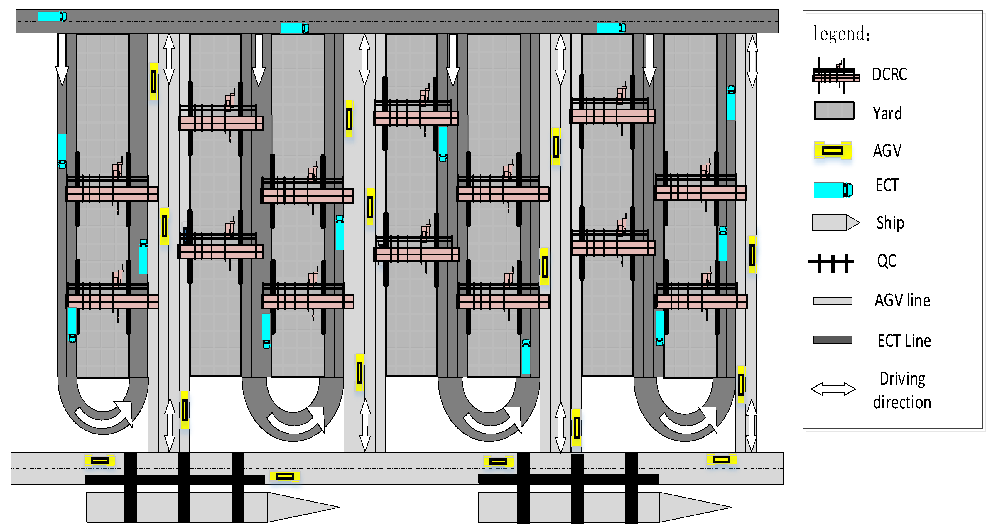
The layout of the U-shaped ACT is shown in Figure 1. In the U-shaped scheme, four AGV lanes are set between every two blocks in the yard. The middle two are overtaking lanes, and the two near the block are operation lanes. Every other block is provided with three “U”-shaped ECT lanes. The middle lane is the overtaking lane, and the two lanes near the block are operation lanes. After loading and unloading the ECT, there is no need to turn around and the truck leaves the container area directly along the U-shaped lanes. There are two exit lanes to avoid congestion.

To study the refined collaborative dispatching method of DCRCs with AGVs and ECTs based on the process optimization of DCRCs, this section is dedicated to optimizing the loading and unloading process of DCRCs to provide a basis for the refined collaborative dispatching of multiple devices.

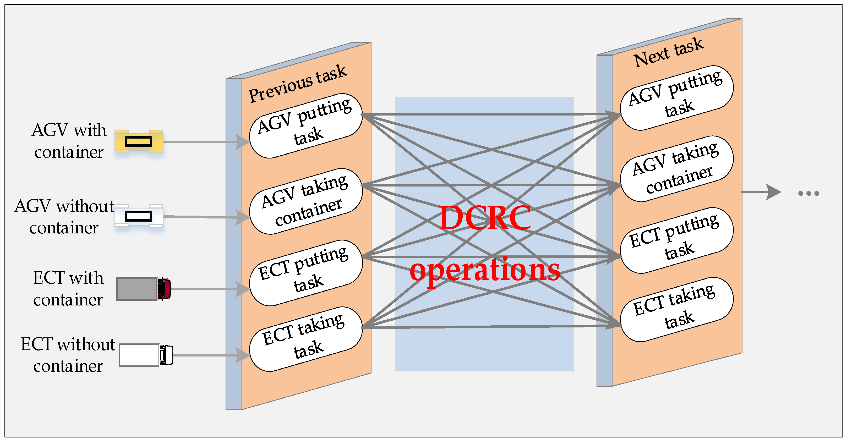
In a U-shaped ACT, DCRCs can work on both sides at any bay with the ECT and the AGV. As the DCRC operation is continuous, different types of tasks in different states take different amounts of time to complete. This time needs to be accurately calculated for different working conditions. To maximize the advantages of U-shaped ACTs and to keep the gantry of DCRCs moving as little as possible, the operating process of the DCRC needs to be optimized. Considering the ECT approach, the DCRC has 16 working conditions in the U-shaped ACT loading and unloading process, as shown in Figure 2.

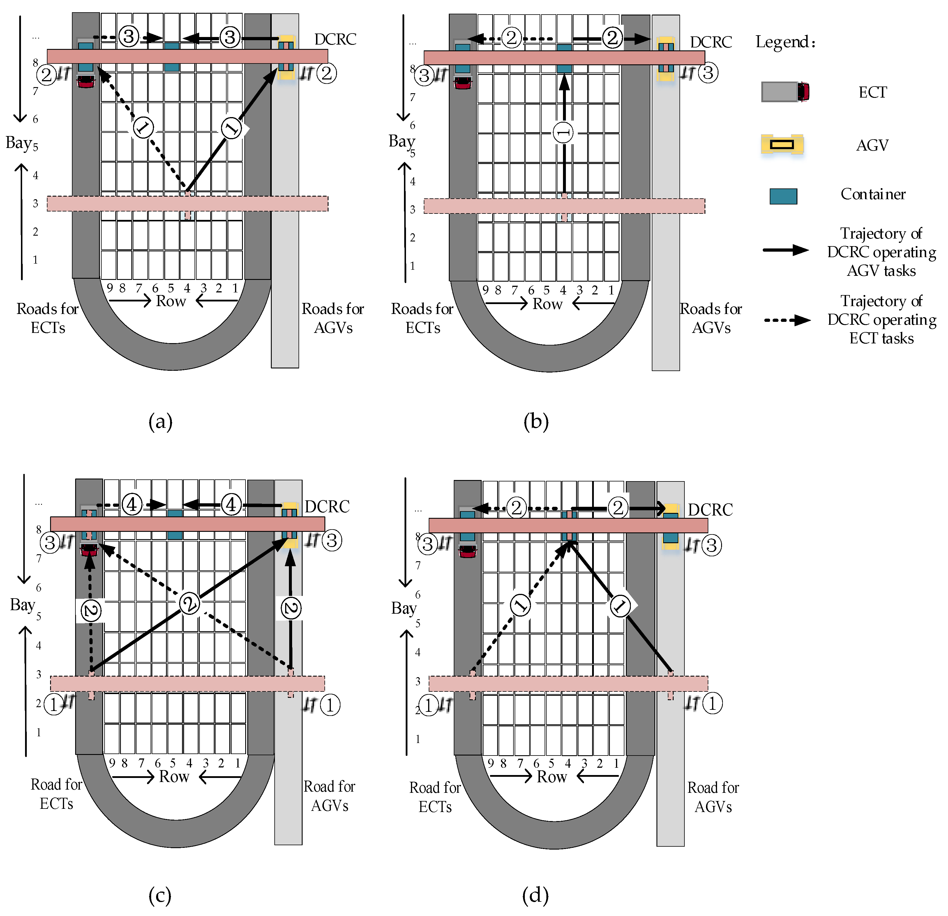
To reduce the energy consumption of the DCRC movement and to allow the DCRC gantry to move as little as possible, the above 16 situations are divided into four modes: putting before putting (PP), putting before taking (PT), taking before putting (TP), and taking before taking (TT), as shown in Figure 3, of which the solid line shows the trajectory of the AGV task for the DCRC operation, and the dashed line shows the trajectory of the ECT task for the DCRC operation. The numbered circles indicate the order of movement for the DCRC gantry and its spreader.

The “PP” mode means that one DCRC has worked on a putting task first, followed by the next putting task. At this time, the motion process of the DCRC is described as follows: (1) The gantry and spreader of the DCRC move from the target position of the previous putting task to the upper edge of the block of the target bay of the next task. (2) The spreader of the DCRC drops down to take the container from the AGV/ECT, completing the task for the AGV/ECT. (3) The spreader of DCRC rises to the upper edge of the block. (4) The spreader of DCRC moves horizontally to the corresponding stack position to put the container, and the DCRC putting task is completed. This mode includes four cases:

• The DCRC continuously handles two putting tasks of AGVs.
• The DCRC handles an AGV putting task after handling the putting task of an ECT.
• The DCRC handles an ECT putting task after handling the putting task of an AGV.
• The DCRC continuously handles two putting tasks of ECTs.

The “PT” mode means that one DCRC first handles a putting task and then handles a taking task. At this time, the motion process of the DCRC is described as follows: (1) The gantry and spreader of the DCRC move from the target position of the previous putting task to the target position of the next taking task. (2) The spreader takes the taking task and moves it to the upper edge of the block. (3) The DCRC’s spreader drops down to place the taking task on the AGV/ECT, and both the AGV/ECT and the DCRC are completed. This mode includes four cases:

• The DCRC handles an AGV taking task after handling the putting task of an AGV.
• The DCRC operates the taking task on the AGV after completing the putting task on the ECT.
• The DCRC operates the taking task on the ECT after completing the putting task on the AGV.
• The DCRC handles an ECT taking task after handling the putting task of an ECT.

The “TP” mode means that one DCRC first handles a taking task and then handles a putting task. At this time, the motion process of the DCRC is described as follows: (1) The DCRC’s spreader ascends from the previous taking task vehicle to the block top. (2) The DCRC’s gantry and spreader move to the upper edge of the block on the side of the next putting task. (3) The spreader of the DCRC drops down to pick up the container from the AGV/ECT, and the AGV/ECT completes its task. (4) The spreader of DCRC rises to the upper edge of the block. (5) The DCRC’s spreader traverse moves to the target stack and places the task in the corresponding bay, at which point the taking task of the DCRC is completed. This model includes four cases:

• The DCRC handles an AGV putting task after handling the taking task of an AGV.
• The DCRC operates the putting task on the AGV after completing the taking task on the ECT.
• The DCRC operates the putting on the ECT after completing the taking task on the AGV.
• The DCRC handles an ECT putting task after handling the taking task of an ECT.

The “TT” mode means that one DCRC has worked on a taking task first, followed by the next taking task. At this time, the motion process of the DCRC is described as follows: (1) The spreader of the DCRC moves up from the interaction point of the previous taking task to the upper edge of the block. (2) The gantry and spreader of the DCRC move to the target position for the next taking task. (3) The spreader picks up the taking task and moves it to the edge of the block on the taking task side. (4) The DCRC’s spreader drops down to place the taking task on the AGV/ECT, and the task of the AGV/ECT and the DCRC is completed. This model includes four cases:

• The DCRC continuously handles two taking tasks of AGVs.
• The DCRC handles an AGV taking task after handling the taking task of an ECT.
• The DCRC handles an ECT taking task after handling the taking task of an AGV.
• The DCRC continuously handles two taking tasks of ECTs.

From the above description, the sequence of operations and target container position for unloading containers, as well as the target container position and reach time for the ECT, are known. However, the DCRC’s subsequent operation and which AGV will go to which QC to operate which container are unknown. Scheduling the AGVs to do the different container tasks and the DCRCs to handle the right tasks at the right time so that the total running time of all the DCRCs is as short as possible will make the U-shaped ACT more efficient. Consequently, we propose a fine-grained collaborative scheduling model for multiple devices that considers the entry of ECTs into the yard.

3.2. Assumptions

(1)

All the containers discussed are 40-foot standard containers.

(2)

The arrival time of the ECT, the target position of the unloading containers, and the position of the loading containers are known.

(3)

The motion of the DCRC is based on the Chebyshev’s motion without considering the interference between them.

(4)

The AGVs, ECTs and DCRCs can work on only one task simultaneously.

(5)

The problem of container turnover is not considered.

(6)

The traveling speeds of the AGV and the ECT and the moving speeds of the DCRC gantry and spreader are fixed values.

(7)

The time for the spreader to travel vertically between the top and bottom of the block is a fixed value.

(8)

The operation time of the AGVs under the QC, the time required for the spreader to grasp the container from the AGVs and ECTs, and the time of the spreader putting at the target position are not counted.

3.3. Notations

(1)

Parameters

$W$	Set of ECT tasks, indexed by $w\in \left(1,2,3,\cdots ,W\right)$
$A$	Set of AGV tasks, indexed by $a\in \left(1,2,3,\cdots ,A\right)$
$A_L$	Set of AGV taking tasks, indexed by $A_{Li}\in \left(1,2,3,\cdots ,A_L\right)$
$W_L$	Set of ECT taking tasks, indexed by $W_{Li}\in \left(1,2,3,\cdots ,W_L\right)$
$I$	Set of AGVs, indexed by $i\in \left(1,2,3,\cdots ,I\right)$
$C$	Set of blocks in yards, indexed by $c,d\in \left(1,2,3,\cdots ,C\right)$
$E$	Set of bays in a block, indexed by $e,s\in \left(1,2,3,\cdots ,E\right)$
$F$	Set of rows in a block, indexed by $f,z\in \left(1,2,3,\cdots ,F\right)$
${\mathrm{c}}_A^{}$	Set of tasks in the block $c$, indexed by ${\mathrm{c}}_p^{},{\mathrm{c}}_q^{}\in \left({\mathrm{c}}_1^{},{\mathrm{c}}_2^{},{\mathrm{c}}_3^{},\cdots ,{\mathrm{c}}_A^{}\right)$
$e_{c_q}$	Bay number of the $qth$ task in block $c$
$f_{c_q}$	Row number of the $qth$ task in block $c$
$v_1$	Speed of the AGV
$v_2$	Speed of the DCRC’s spreader
$v_3$	Speed of the DCRC’s gantry
$M$	A very large positive number
$J$	Length of a block
$K$	Width of a block
$BL$	Length of a bay
$EW$	Length of a row
$T{Q}_c$	Time matrix of AGVs traveling between the QC and block $c$
$T_{cd}$	Time matrix of AGVs traveling between the block $c$ and block $d$
$T{w}_c$	Arrival time of the $wth$ ECT in block $c$
$TT$	Time required for DCRC’s spreader to travel vertically

(2)

Decision variables

$t{i}_1^{c_q}$	The moment when the AGV receives the $qth$ task of block $c$ at the QC
$t{i}_2^{c_q}$	The moment when the AGV transports the $qth$ task of block $c$ to the end of the block
$t{i}_3^{c_q}$	The moment when the AGV arrives at the designated bay of the $qth$ task of block $c$
$t{i}_{end}^{c_q}$	The moment when the AGV finishes the $qth$ task in block $c$
$t{d}_1^{c_q}$	The moment when the spreader moves across to the edge of the block
$t{d}_2^{c_q}$	The moment the spreader drops to the vehicle interaction position
$t{d}_3^{c_q}$	The moment the spreader moves up to the edge of the block
$t{d}_4^{c_q}$	The moment the spreader moves across to the target position
$t{d}_{end}^{c_q}$	The moment when the DCRC finish the $qth$ task in block $c$
$ti{d}_{inter}^{c_q}$	The moment of interaction of the AGV with the spreader for the $qth$ task in block $c$
${\lambda }_{c_q}$	When the $qth$ task of block $c$ is an AGV task ${\lambda }_{c_q}=1$, otherwise ${\lambda }_{c_q}=0$
${\pi }_{c_q}$	When the $qth$ task of block $c$ is a putting task ${\pi }_{c_q}=1$, otherwise ${\pi }_{c_q}=0$
${\theta }_{d_p}^{c_q}$	When the AGV finishes processing the $qth$ putting task in block $c$ and goes to process the $qth$ taking task in block $d$, ${\theta }_{d_p}^{c_q}=1$; otherwise, ${\theta }_{d_p}^{c_q}=0$
${\partial }_{d_p}^{c_q}$	When the AGV finishes processing the $qth$ taking task in block $c$ and goes to process the $qth$ putting task in block $d$, ${\partial }_{d_p}^{c_q}=1$; otherwise, ${\partial }_{d_p}^{c_q}=0$
${\epsilon }_i^{c_{pq}}$	When the AGV $i$ operates the $qth$ putting task in block $c$ and then continues to operate the $qth$ taking task in this block, ${\epsilon }_i^{c_{pq}}=1$;; otherwise, ${\epsilon }_i^{c_{pq}}=0$
${\sigma }_{c_q}^{\begin{array}{c}i\end{array}}$	When AGV $i$ performs the task of the $qth$ container in block $c$, ${\sigma }_{c_q}^{\begin{array}{c}i\end{array}}=1$; otherwise, ${\sigma }_{c_q}^{\begin{array}{c}i\end{array}}=0$
${\varphi }_{A_{Li}}^{e_{c_q},f_{c_q}}$	When the task in block $c$ of bay $b$, row $r$ is the $ith$ taking task of AGV, ${\varphi }_{A_{Li}}^{e_{c_q},f_{c_q}}=1$; otherwise, ${\varphi }_{A_{Li}}^{e_{c_q},f_{c_q}}=0$
${\Omega }_{W_{Li}}^{e_{c_q},f_{c_q}}$	When the task in block $c$ of bay $b$, row $r$ is the $ith$ taking task of ECT, ${\Omega }_{W_{Li}}^{e_{c_q},f_{c_q}}=1$; otherwise, ${\Omega }_{W_{Li}}^{e_{c_q},f_{c_q}}=0$.

3.4. Model

To solve the collaborative scheduling problem of DCRCs and AGVs, this paper proposes a mixed-integer programming model with the goal of achieving the minimum total running time for all DCRCs.

$$Z={\displaystyle \sum _{c_q\in c_A,c\in C}\max \left\{t_{end}^{c_q}\right\}}$$

(1)

Equation (1) is the objective function that minimizes the sum of the total occupied time of all DCRCs.

$${\displaystyle \sum _{c,d\in \mathrm{C}}^{}{\displaystyle \sum _{\begin{array}{l}\begin{array}{c}\begin{array}{c}\begin{array}{c}\end{array}\end{array}\end{array}{c}_q\in c_A\\ d_p\in d\end{array}}^{}{\theta }_{d_p}^{c_q}=1}} \forall i\in I$$

(2)

$${\displaystyle \sum _{c,d\in \mathrm{C}}^{}{\displaystyle \sum _{\begin{array}{l}\begin{array}{c}\begin{array}{c}\begin{array}{c}\end{array}\end{array}\end{array}{c}_q\in c\\ d_p\in d\end{array}}^{}{\partial }_{d_p}^{c_q}=1}} \forall i\in I$$

(3)

$${\displaystyle \sum _{c\in C}^{}{\displaystyle \sum _{{\mathrm{c}}_q\in {\mathrm{c}}_A}^{}{\sigma }_{c_q}^{\begin{array}{c}i\end{array}}=1}} \forall i\in I$$

(4)

$${\displaystyle \sum _{i\in I}^{}{\sigma }_{c_q}^{\begin{array}{c}i\end{array}}=1} \forall c\in C,c_q\in c_A$$

(5)

$${\displaystyle \sum _{c\in C}^{}{\displaystyle \sum _{{\mathrm{c}}_q\in {\mathrm{c}}_A}^{}{\varphi }_{A_{Li}}^{e_{c_q},f_{c_q}}=1}} \forall A_{Li}\in A_L$$

(6)

$${\displaystyle \sum _{c\in C}^{}{\displaystyle \sum _{{\mathrm{c}}_q\in {\mathrm{c}}_A}^{}{\mathsf{\Omega }}_{W_{Li}}^{e_{c_q},f_{c_q}}=1}} \forall W_{Li}\in W_L$$

(7)

Constraints (2)–(7) ensure the uniqueness of the task for the AGV. Constraint (2) provides for the AGV performing a taking task after completing a putting task. Constraint (3) requires that the AGV performs a putting task after completing a taking task. Constraints (2) and (3) guarantee the integrity of the loading and unloading processes. Constraint (4) assures that each task is operated by one and only one AGV. Constraint (5) ensures that each AGV handles only one task simultaneously. Constraint (6) guarantees that each AGV taking task has a unique taking sequence corresponding to it. Constraint (7) assures that each ECT taking task has a unique taking sequence corresponding to it.

$$t{i}_1^{c_q}+T{Q}_c-t{i}_2^{c_q}+\left(1-{\pi }_{c_q}\right)\cdot M\le 0 \begin{array}{l}\forall c\in C,c_q\in c_A\\ \forall i\in I\end{array}$$

(8)

$$t{i}_2^{c_q}+\frac{BL\cdot e_{c_q}}{v_1}-t{i}_3^{c_q}+\left(1-{\pi }_{c_q}\right)\cdot M\le 0 \begin{array}{l}\forall c\in C,c_q\in c_A\\ \forall i\in I\end{array}$$

(9)

$$t{i}_{end}^{c_q}+\frac{\left(e_{c_q}-e_{c_p}\right)\cdot BL}{v_1}-t{i}_3^{c_q}+{\pi }_{c_p}\cdot M+\left(1-{\epsilon }_i^{c_{pq}}\right)\cdot M\le 0 \begin{array}{l}\forall c\in C,c_q,c_p\in c_A\\ \forall i\in I\end{array}$$

(10)

$$t{i}_{end}^{c_q}+\frac{J+T_{cd}+e_{c_q}\cdot BL}{v_1}-t{i}_3^{d_p}+{\pi }_{d_p}\cdot M+{\epsilon }_{c_{pq}}^{}\cdot M\le 0 \begin{array}{l}\forall c,d\in C,c_q\in c_A\\ \forall d_p\in d_A,i\in I\end{array}$$

(11)

Constraints (8)–(11) represent the time relationship at the horizontal transport link when the AGV releases the putting task. Constraint (8) indicates the relationship between the moment when the AGV receives the $qth$ task from QC to the front end of block $c$. Constraint (9) represents the moment the AGV transports the $qth$ task of block $c$ to the front of the block, concerning the moment the task is delivered to the target bay $e$. Constraints (10) and (11) indicate the relationship between the moment the AGV completes the previous putting task and the moment it starts the next taking task. Constraint (10) represents the time relationship between the AGV going to the same block to take the container after it has completed the putting task. Constraint (11) represents the time relationship between the AGV going to a different block to take a container after it has completed the putting task.

$$ti{d}_{inter}^{c_q}+\frac{BL\cdot e_{c_q}}{v_1}-t{i}_2^{c_q}+\left(1-{\pi }_{c_q}\right)\cdot M\le 0 \begin{array}{l}\forall c\in C,i\in I\\ \forall c_q\in c_A\end{array}$$

(12)

$$t{i}_3^{c_q}+T{Q}_c-t{i}_1^{c_q}+\left(1-{\pi }_{c_q}\right)\cdot M\le 0 \begin{array}{l}\forall c\in C,i\in I\\ \forall c_q\in c_A\end{array}$$

(13)

$$t{i}_1^{c_q}-t{i}_{end}^{c_q}=0 \begin{array}{l}\forall c\in C,i\in I\\ \forall c_q\in c_A\end{array}$$

(14)

$$t{i}_{end}^{c_q}+\left(1-{\pi }_{c_q}\right)\cdot M-t{i}_1^{d_p}\cdot \left({\pi }_{d_p}-1\right)\le 0 \begin{array}{l}\forall c,d\in C,i\in I\\ \forall c_q\in c_A,d_p\in d_A\end{array}$$

(15)

Constraints (12)–(14) indicate the time relationship between the horizontal transport links when the AGV performs the taking task. Constraint (12) indicates the time relationship in which the AGV runs the $qth$ task of block c from the block bay position to the front of the block. Constraint (13) means the relationship between the moment when the AGV runs the $qth$ task of block $c$ from the front of the block to the QC. Constraint (14) describes the moment at which the AGV has completed its operation, when it reaches the QC with the $qth$ task of block $c$ loading onto the vessel. Constraint (15) concerns the time relationship between when the AGV completes the $qth$ taking task in the previous block $e$ and when it starts the $pth$ putting task in block $d$.

$$\left[t{d}_{end}^{c_{q-1}}+\max \left(\begin{array}{l}\frac{BL\cdot \left|e_{c_q}-e_{c_{q-1}}\right|}{v_2},\\ \frac{EW\cdot f_{c_q-1}\cdot {\lambda }_{c{t}_q}+\left(K-EW\cdot e_{c_{q-1}}\right)\cdot \left(1-{\lambda }_{c{t}_q}\right)}{v_3}\end{array}\right)-t{d}_1^{c_q}\right]\cdot {\pi }_{c_{q-1}}\cdot {\pi }_{c_q}\le 0 \begin{array}{l}\forall c\in C,\\ \forall c_{q-1},c_q\in c_A\end{array}$$

(16)

$$\left(t{d}_1^{c_q}+TT-t{d}_2^{c_q}\right)\cdot {\pi }_{c_{q-1}}\cdot {\pi }_{c_q}\le 0 \begin{array}{l}\forall c\in C,\\ \forall c_{q-1},c_q\in c_A\end{array}$$

(17)

$$\left[ti{d}_{inter}^{c_q}-\max \left(t{i}_3^{c_q}\cdot {\lambda }_{c_q},T{w}_c\cdot \left(1-{\lambda }_{c_q}\right),t{d}_2^{c_q}\right)\right]\cdot {\pi }_{c_{q-1}}\cdot {\pi }_{c_q}=0 \begin{array}{l}\forall c\in C\\ \forall i\in I,w\in W\\ \forall c_{q-1},c_q\in c_A\end{array}$$

(18)

$$\left(t{i}_{end}^{c_q}-ti{d}_{inter}^{c_q}\right)\cdot {\lambda }_{c_q}\cdot {\pi }_{c_{q-1}}\cdot {\pi }_{c_q}=0 \begin{array}{l}\forall c\in C,i\in I\\ \forall c_{q-1},c_q\in c_A\end{array}$$

(19)

$$\left(ti{d}_{inter}^{c_q}+TT-t{d}_3^{c_q}\right)\cdot {\pi }_{c_{q-1}}\cdot {\pi }_{c_q}\le 0 \begin{array}{l}\forall c\in C,i\in I\\ \forall c_{q-1},c_q\in c_A\end{array}$$

(20)

$$\left[t{d}_3^{c{t}_q}+\frac{EW\cdot f_{c_q}\cdot {\lambda }_{c_q}+\left(K-EW\cdot f_{c_q}\right)\cdot \left(1-{\lambda }_{c_q}\right)}{v_3}-t{d}_4^{c_q}\right]\cdot {\pi }_{c_{q-1}}\cdot {\pi }_{c_q}\le 0 \begin{array}{l}\forall c\in C,\\ \forall c_{q-1},c_q\in c_A\end{array}$$

(21)

$$\left(t{d}_{end}^{c_q}-t{d}_4^{c_q}\right)\cdot {\pi }_{c_{q-1}}\cdot {\pi }_{c_q}=0 \begin{array}{l}\forall c\in C,\\ \forall c_{q-1},c_q\in c_A\end{array}$$

(22)

Constraints (16)–(22) indicate the time relationship when the DCRC is operating in “PP” mode. Constraint (16) represents the time relationship between the end of the previous putting task of the DCRC and the spreader moving across to the edge of the block where the current putting task is positioned. Constraint (17) describes the time taken for the spreader to descend from above the block to the interaction point. Constraint (18) shows that the moment of interaction is the maximum of the moment when the spreader drops to the interaction point and the arrival time of the AGV or the ECT. Constraint (19) states that the DCRC and the AGV will interact when the AGV has finished its block delivery putting task. Constraint (20) means the moment when the spreader returns to the edge of the block after lifting the container. Constraint (21) represents the time relationship between the spreader running from the edge of the block on both sides to the specified stack. Constraint (22) means the moment when the DCRC has completed the current putting task.

$$t{d}_{end}^{c_{q-1}}+\max \left(\frac{BL\cdot \left|e_{c_q}-e_{c_{q-1}}\right|}{v_2},\frac{EW\cdot \left|f_{c_q}-f_{c_{q-1}}\right|}{v_3}\right)-t{d}_4^{c_q}\cdot {\pi }_{c_{q-1}}\cdot \left(1-{\pi }_{c_q}\right)\le 0 \begin{array}{l}\forall c\in C,\\ \forall c_{q-1},c_q\in c_A\end{array}$$

(23)

$$\left(t{d}_4^{c{t}_q}+\frac{BL\cdot f_{c_q}\cdot {\lambda }_{c_q}+\left(K-BL\cdot f_{c_q}\right)\cdot \left(1-{\lambda }_{c_q}\right)}{v_3}-t{d}_1^{c{t}_q}\right)\cdot {\pi }_{c_{q-1}}\cdot \left(1-{\pi }_{c_q}\right)\le 0 \begin{array}{l}\forall c\in C,\\ \forall c_{q-1},c_q\in c_A\end{array}$$

(24)

$$\left(t{d}_1^{c_q}+TT-t{d}_2^{c_q}\right)\cdot {\pi }_{c_{q-1}}\cdot \left(1-{\pi }_{c_q}\right)\le 0 \begin{array}{l}\forall c\in C,\\ \forall c_{q-1},c_q\in c_A\end{array}$$

(25)

$$ti{d}_{inter}^{c_q}-\max \left(t{d}_2^{c_q},T{w}_c\right)\cdot {\lambda }_{c_q}\cdot {\pi }_{c_{q-1}}\cdot \left(1-{\pi }_{c_q}\right)=0 \begin{array}{l}\forall c\in C\\ \forall i\in I,w\in W\\ \forall c_{q-1},c_q\in c_A\end{array}$$

(26)

$$t{d}_{end}^{c_q}-\max \left(t{d}_2^{c_q},T{w}_c\right)\cdot {\pi }_{c_{q-1}}\cdot \left(1-{\pi }_{c_q}\right)=0 \begin{array}{l}\forall c\in C\\ \forall i\in I,w\in W\\ \forall c_{q-1},c_q\in c_A\end{array}$$

(27)

Constraints (23)–(27) indicate the time relationship when the DCRC is operating in “PT” mode. Constraint (23) represents the time relationship between the previous putting task ending and the spreader reaching the position of the current taking task. Constraint (24) represents the time relationship between the spreader picking up the putting task and moving across to the edge of the block where the vehicle is positioned. Constraint (25) represents the moment when the spreader reaches the edge of the block and drops down to the AGV or the ECT interaction position. Constraint (26) indicates that if the task is an AGV taking task, the moment of interaction between the AGV and the DCRC is the maximum of the moment when the spreader drops to the point of interaction with the AGV and the moment of arrival of the AGV. Constraint (27) indicates that the end of the taking task of the AGV/ECT and the DCRC is the maximum of the moment when the spreader reaches the point of interaction and the moment of arrival of the AGV or the ECT.

$$t{d}_{end}^{c_{q-1}}+TT-t{d}_3^{c_q}\cdot \left(1-{\pi }_{c_{q-1}}\right)\cdot {\pi }_{c_q}\le 0 \begin{array}{l}\forall c\in C,\\ \forall c_{q-1},c_q\in c_A\end{array}$$

(28)

$$\left[t{d}_3^{c_q}+\max \left(\frac{EW\cdot \left|e_{c_q}-e_{c_{q-1}}\right|}{v_2},\frac{K}{v_3}\cdot \left|{\lambda }_{c_{q-1}}-{\lambda }_{c_q}\right|\right)-t{d}_1^{c_q}\right]\cdot \left(1-{\pi }_{c_{q-1}}\right)\cdot {\pi }_{c_q}\le 0 \begin{array}{l}\forall c\in C,\\ \forall c_{q-1},c_q\in c_A\end{array}$$

(29)

$$\left(t{d}_1^{c_q}+TT-t{d}_2^{c_q}\right)\cdot \left(1-{\pi }_{c_{q-1}}\right)\cdot {\pi }_{c_q}\le 0 \begin{array}{l}\forall c\in C,\\ \forall c_{q-1},c_q\in c_A\end{array}$$

(30)

$$\left[ti{d}_{inter}^{c_q}-\max \left(t{i}_3^{c_q}\cdot {\lambda }_{c_q},T{w}_c\cdot \left(1-{\lambda }_{c_q}\right),t{d}_2^{c_q}\right)\right]\cdot \left(1-{\pi }_{c_{q-1}}\right)\cdot {\pi }_{c_q}=0 \begin{array}{l}\forall c\in C\\ \forall i\in I,w\in W\\ \forall c_{q-1},c_q\in c_A\end{array}$$

(31)

$$\left(t{i}_{end}^{c_q}-ti{d}_{inter}^{c_q}\right)\cdot {\lambda }_{c_q}\cdot \left(1-{\pi }_{c_{q-1}}\right)\cdot {\pi }_{c_q}=0 \begin{array}{l}\forall c\in C,i\in I\\ \forall c_{q-1},c_q\in c_A\end{array}$$

(32)

$$\left(ti{d}_{inter}^{c_q}+TT-t{d}_3^{c_q}\right)\cdot \left(1-{\pi }_{c_{q-1}}\right)\cdot {\pi }_{c_q}\le 0 \begin{array}{l}\forall c\in C,i\in I\\ \forall c_{q-1},c_q\in c_A\end{array}$$

(33)

$$\left[t{d}_3^{c{t}_q}+\frac{EW\cdot f_{c_q}\cdot {\lambda }_{c_q}+\left(K-EW\cdot f_{c_q}\right)\cdot \left(1-{\lambda }_{c_q}\right)}{v_3}-t{d}_4^{c_q}\right]\cdot \left(1-{\pi }_{c_{q-1}}\right)\cdot {\pi }_{c_q}\le 0 \begin{array}{l}\forall c\in C,\\ \forall c_{q-1},c_q\in c_A\end{array}$$

(34)

$$\left(t{d}_{end}^{c_q}-t{d}_4^{c_q}\right)\cdot \left(1-{\pi }_{c_{q-1}}\right)\cdot {\pi }_{c_q}=0 \begin{array}{l}\forall c\in C,\\ \forall c_{q-1},c_q\in c_A\end{array}$$

(35)

Constraints (28)–(35) indicate the time relationship when the DCRC is operating in “TP” mode. Constraint (28) means the moment the spreader is lifted above the block after completing the previous putting task. Constraint (29) indicates the time relationship after the spreader has been lifted and the spreader reaches the corresponding bay at the next task’s block side. Constraint (30) represents the time relationship between the spreader leaving the block’s edge and interacting with the vehicle. Constraint (31) indicates that the interaction time is the maximum of the moment when the spreader sags to the interaction point and the arrival time of the AGV or the ECT. Constraint (32) indicates that, if the task is an AGV putting task, the moment of interaction between the DCRC and the AGV is when the AGV discharge task is completed. Constraint (33) represents the moment when the spreader returns to the edge of the block after picking up the container. Constraint (34) represents the time relationship when the spreader runs from the edges on the sides of the block to the designated stack. Constraint (35) indicates the moment when the DCRC has completed its putting task.

$$\left(t{d}_{end}^{c_{q-1}}+TT-t{d}_3^{c_q}\right)\cdot \left(1-{\pi }_{c_{q-1}}\right)\cdot \left(1-{\pi }_{c_q}\right)\le 0 \begin{array}{l}\forall c\in C,\\ \forall c_{q-1},c_q\in c_A\end{array}$$

(36)

$$\begin{array}{l}t{d}_3^{c_q}+\max \left(\begin{array}{l}\frac{BL\cdot \left|e_{c_q}-e_{c_{q-1}}\right|}{v_2},\\ \frac{EW\cdot f_{c_q}\cdot {\lambda }_{c_{q-1}}+\left(K-EW\cdot f_{c_q}\right)\cdot \left(1-{\lambda }_{c_{q-1}}\right)}{v_3}\end{array}\right)-\\ t{d}_4^{c{t}_q}\cdot \left(1-{\pi }_{c_{q-1}}\right)\cdot \left(1-{\pi }_{c_q}\right)\le 0\end{array}\begin{array}{l}\forall c\in C,\\ \forall c_{q-1},c_q\in c_A\end{array}$$

(37)

$$\left(t{d}_4^{c_q}+\frac{EW\cdot f_{c_q}\cdot {\lambda }_{c_q}+\left(K-EW\cdot f_{c_q}\right)\cdot \left(1-{\lambda }_{c_q}\right)}{v_3}-t{d}_1^{c_q}\right)\cdot \left(1-{\pi }_{c_{q-1}}\right)\cdot \left(1-{\pi }_{c_q}\right)\le 0 \begin{array}{l}\forall c\in C,\\ \forall c_{q-1},c_q\in c_A\end{array}$$

(38)

$$\left(t{d}_1^{c_q}+TT-t{d}_2^{c_q}\right)\cdot \left(1-{\pi }_{c_{q-1}}\right)\cdot \left(1-{\pi }_{c_q}\right)\le 0 \begin{array}{l}\forall c\in C,\\ \forall c_{q-1},c_q\in c_A\end{array}$$

(39)

$$ti{d}_{inter}^{c_q}-\max \left(t{d}_2^{c_q},T{w}_c\right)\cdot {\lambda }_{c_q}\cdot \left(1-{\pi }_{c_{q-1}}\right)\cdot \left(1-{\pi }_{c_q}\right)=0 \begin{array}{l}\forall c\in C\\ \forall i\in I,w\in W\\ \forall c_{q-1},c_q\in c_A\end{array}$$

(40)

$$t{d}_{end}^{c{t}_q}-\max \left(t{d}_2^{c_q},T{w}_c\right)\cdot \left(1-{\pi }_{c_{q-1}}\right)\cdot \left(1-{\pi }_{c_q}\right)=0 \begin{array}{l}\forall c\in C,w\in W\\ \forall c_{q-1},c_q\in c_A\end{array}$$

(41)

Constraints (36)–(41) indicate the time relationship when the DCRC is operating in “TT” mode. Constraint (36) represents the relationship between the moment when the previous taking task ends and the moment when the spreader moves up to the edge of the block. Constraint (37) represents the time relationship between the arrival of the spreader from the edge of the block of the previous taking task to the container position to be taken. Constraint (38) represents the time relationship between the moment when the spreader takes the taking task to be lifted and the moment when it moves across to the edge of the block for the taking task to be lifted. Constraint (39) shows when the spreader reaches the edge of the block and when it drops down to the position where the vehicle can interact with it. Constraint (40) indicates that, if the task is an AGV taking task, this interaction moment is the maximum of the moment when the spreader is dropped at the interaction point of the AGV and the arrival moment of the AGV. Constraint (41) represents that the greater time between when the spreader drops to the point of interaction and the time of arrival of the AGV/ECT is the end time of the DCRC task.

$$t{i}_1^{c_q},t{i}_2^{c_q},t{i}_3^{c_q},t{i}_{end}^{c_q},t{d}_1^{c_q},t{d}_2^{c_q},t{d}_3^{c_q},t{d}_4^{c_q},t{d}_{end}^{c_q},ti{d}_{inter}^{c_q}\ge 0 \forall c\in C,c_q\in c_A$$

(42)

Constraint (42) defines the range of parameters of the decision variables.

4. Proposed Algorithm

As the logic of the model studied in this paper is more complex and there are many optional loading and unloading points, the chosen algorithm needs to be practical. Genetic algorithms (GA) have good global search capabilities and excellent robustness, and several scholars have verified the reliability of GA for equipment scheduling problems [36,44,45].

Because each bay of the block in the U-shaped scheme can perform loading and unloading tasks, the available optional point is dozens of times that of the end operation scheme. To better fit the actual operation of the port, the refined collaborative scheduling model of the U-shaped ACT in the loading and unloading process established in this paper considers more operation modes and more complex logical relationships. This paper proposes the adaptive co-evolutionary genetic algorithm (ACGA) to solve the model better. The ACGA uses the idea of two-population coevolution to improve population diversity, and improves the convergence speed of the algorithm through adaptive dynamic adjustment of parameters. This paper uses two rules as stop criteria to ensure reasonable calculation time and accuracy of results: when the optimal fitness value (OFV) remains unchanged for several generations or the number of iterations reaches the maximum algebra, the algorithm stops. The flow of the ACGA is shown in Figure 4.

4.1. Chromosome Coding

The algorithm uses an integer coding approach where one chromosome represents the sequence of operations for a set of AGVs, i.e., a candidate solution. In the above hypothetical model, the target container position and sequence of operations for each container are known, and the ECT’s type of operation and arrival time are known. The order in which AGV will serve the QC and the type of task for the next DCRC operation are unknown. The task sequence of the AGVs is scheduled to determine the type of operation of the DCRC in conjunction with the arrival time of the ECTs.

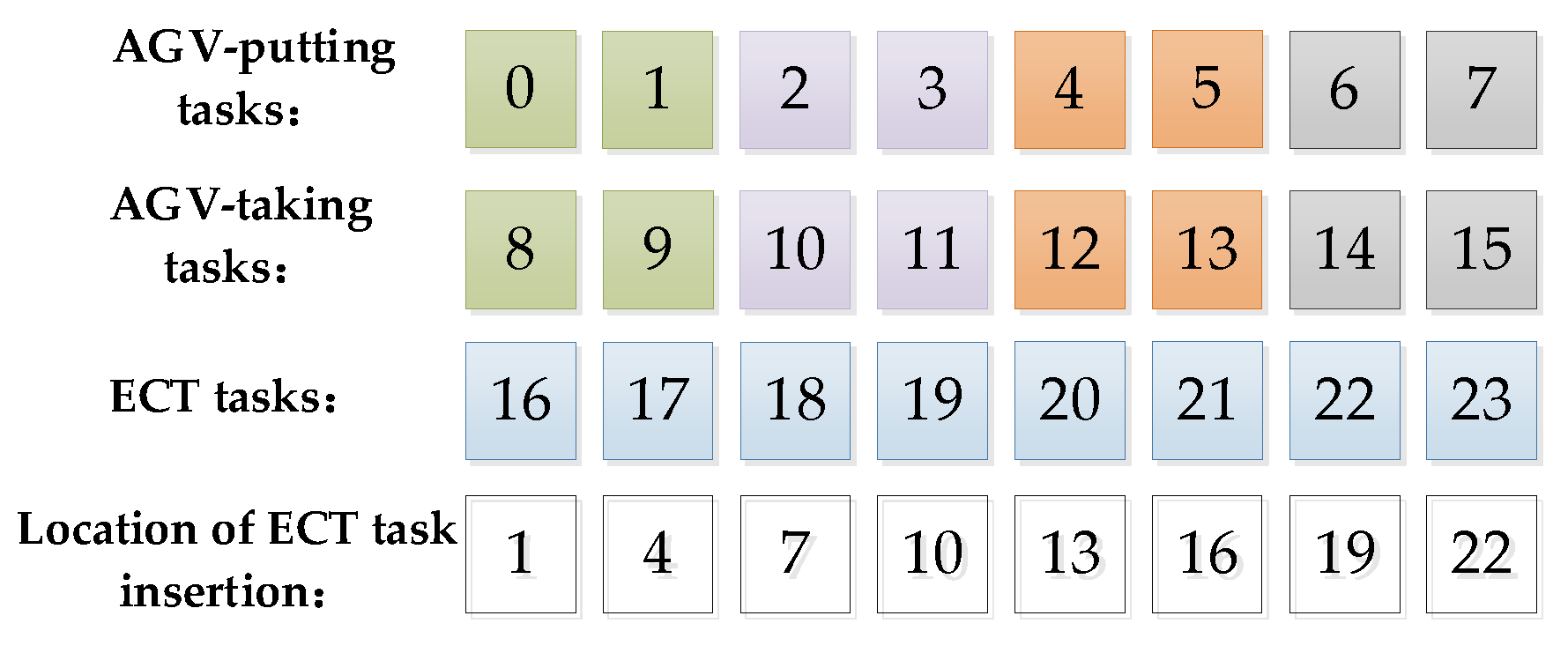
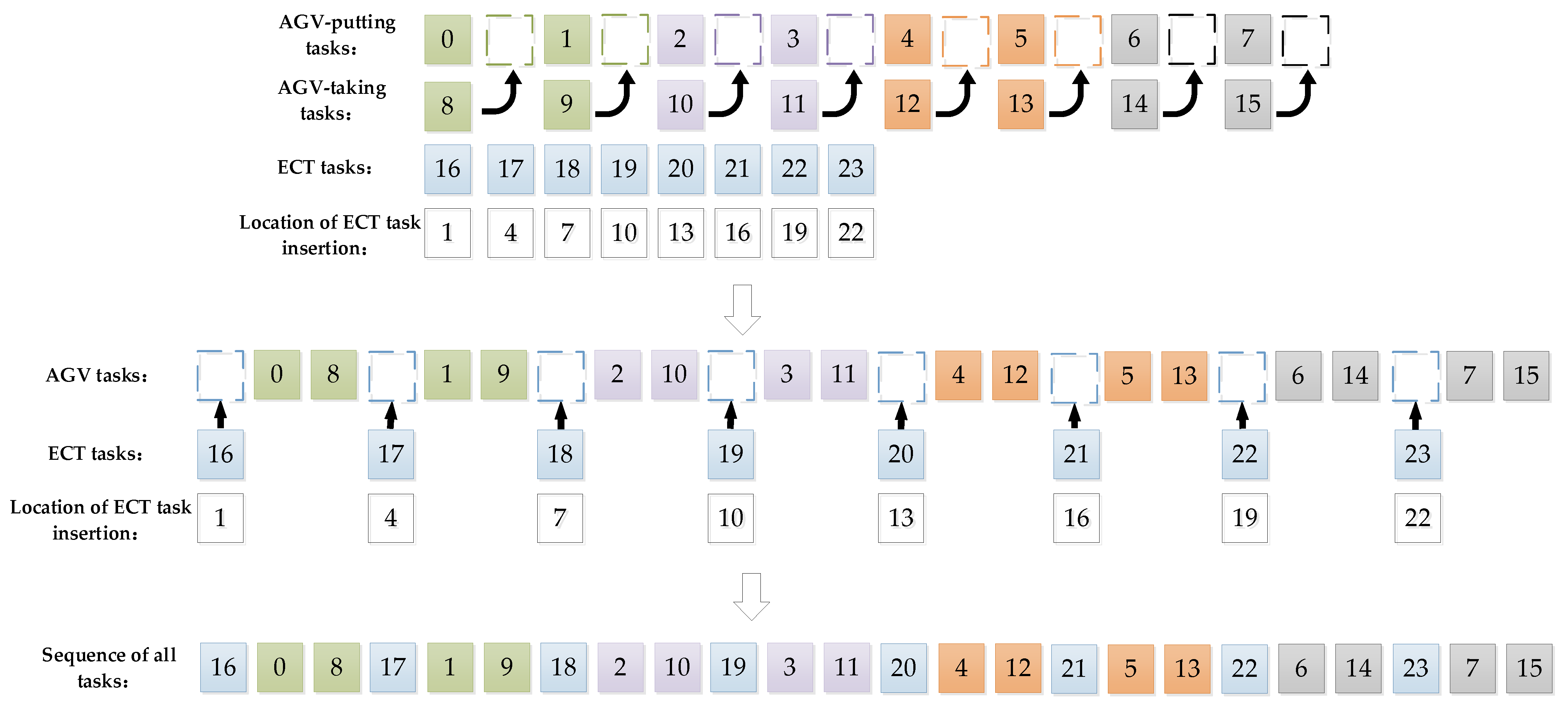
To distinguish between the AGV task, the ECT task, and the DCRC task, this paper is coded with a multi-layer chromosome in the form of a task assignment. The initial chromosome is shown in Figure 5. It is assumed that there are two DCRCs and four AGVs. Eight AGV-putting tasks are denoted by the numbers 0–7. Eight AGV-taking tasks are denoted by the numbers 8–15. Four ECT-putting tasks are denoted by the numbers 16–19. Four ECT-taking tasks are denoted by the numbers 20–23. All odd-numbered tasks are those of DCRC 1, and even-numbered tasks are those of DCRC 2. The green, purple, orange, and grey genes indicate the tasks of AGV 1, AGV 2, AGV 3, and AGV 4, respectively.

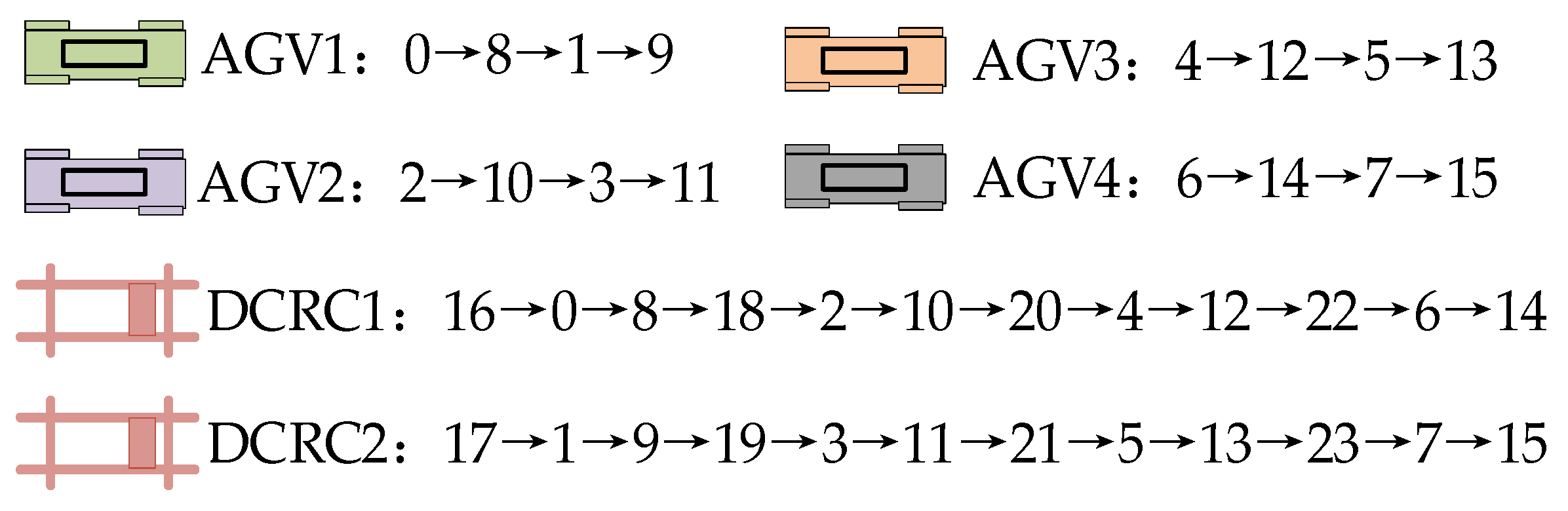
As shown in Figure 5, the first chromosome layer is for AGV-putting tasks. The second chromosome layer is for AGV-taking tasks. Since the AGV always performs a putting task and then goes to a taking task, the second chromosome layer is inserted sequentially after the genes in the first chromosome layer. The third chromosome layer is for ECT tasks. The position in the chromosome of the ECT task at the corresponding position in the third layer is indicated by the fourth layer of chromosomes. The final obtained initial chromosome corresponds to the sequence of jobs, as shown in Figure 6. The task assignments of the AGV and DCRC for this chromosome are shown in Figure 7.

4.2. Coevolution

Coevolution was first proposed by Ehrlich and Raven. In this process, different populations have different evolutionary goals, and they can complement each other with information, have strong global search ability, and overcome the phenomenon of a single population and premature convergence in the later stage of the GA [46,47,48].

The first illustration of the degree of variation in the task order is given by assuming that there are $V$ AGVs and $Y$ containers. A population has X task orders, and the degree of variation between task orders $x_b$ and $x_m$ is:

$$Q=\frac{1}{Y}{\displaystyle \sum _{y=1}^Y\lambda \begin{array}{ccc}& & \end{array}if\left\{\begin{array}{c}{x}_y^b=x_y^m,\lambda =0\\ x_y^b\ne x_y^m,\lambda =1\end{array}\right.},\begin{array}{c}\end{array}{x}_y^b,x_y^m\in V$$

(43)

$x_y^b$ denotes the $y\mathrm{t}\mathrm{h}$ task sequence number of task sequence $b$, resulting in the shortest total running time of the current DCRCs. $x_y^m$ is the $y\mathrm{t}\mathrm{h}$ task sequence number of the $m\mathrm{t}\mathrm{h}$ task sequence. The larger the value of $Q$, the greater the degree of difference between the total running time of the DCRC represented by that task sequence and the current shortest total running time.

After generating the initial task order population, as coded above, this task order population is divided into a sprint population and a supplementary population. The objective function for the sprint population is $Z={\displaystyle \sum _{a\in A}}{\displaystyle \sum _{w\in W}}\min (Z_1+Z_2)$, i.e., the shortest running time for all DCRCs, to guide the population to converge as soon as possible. The objective function of the supplementary population is $Q*Z$, which aims to maintain population diversity, complement the primary population, and avoid premature maturation of the algorithm. When the two task sequential populations have completed the crossover and variation operations, respectively, they are ranked by the shortest operation time of the respective task populations. The top 2/3 of the sprint population and the top 1/3 of the complementary population are selected from lowest to highest to form a new task population. The two populations are independent of each other and can be made computationally more efficient by using parallel computing methods during the calculation.

4.3. Adaptive Crossover and Mutation

The probability of changing the order of tasks determines the richness of the task population. By adaptively changing the probability of crossover and mutation, faster and more accurate convergence to the shortest total running time of a DCRC can be achieved. For example, the probability of crossover and mutation becomes larger when the degree of variation in the minimum total running time of the task order in the task population is low. When the degree of variation is high, the probability of crossover and mutation is low. The adaptive probability adjustment expression for crossover and variation is:

$$if\begin{array}{c}\end{array}\arcsin \left(\frac{f_{ave}}{f_{\max }}\right)<\pi /6\left\{\begin{array}{l}{P}_{\mathrm{c}}=k_1\frac{\arcsin \left(\frac{f_{ave}}{f_{\max }}\right)}{\pi /2}\\ P_m=k_2\left(1-\frac{\arcsin \left(\frac{f_{ave}}{f_{\max }}\right)}{\pi /2}\right)\end{array}\right.$$

(44)

$$if\begin{array}{c}\end{array}\arcsin \left(\frac{f_{ave}}{f_{\max }}\right)\ge \pi /6\left\{\begin{array}{l}{P}_{\mathrm{c}}=k_1\left(1-\frac{\arcsin \left(\frac{f_{ave}}{f_{\max }}\right)}{\pi /2}\right)\\ P_m=k_2\frac{\arcsin \left(\frac{f_{ave}}{f_{\max }}\right)}{\pi /2}\end{array}\right.$$

(45)

$p_c$ and $p_m$ are the crossover probability and mutation probability; $k_1$ and $k_2$ are random numbers between [0, 1]; and $f_{max}$ and $f_{avg}$ are the maximum and average values of the DCRC’s shortest operating times in the task population, respectively.

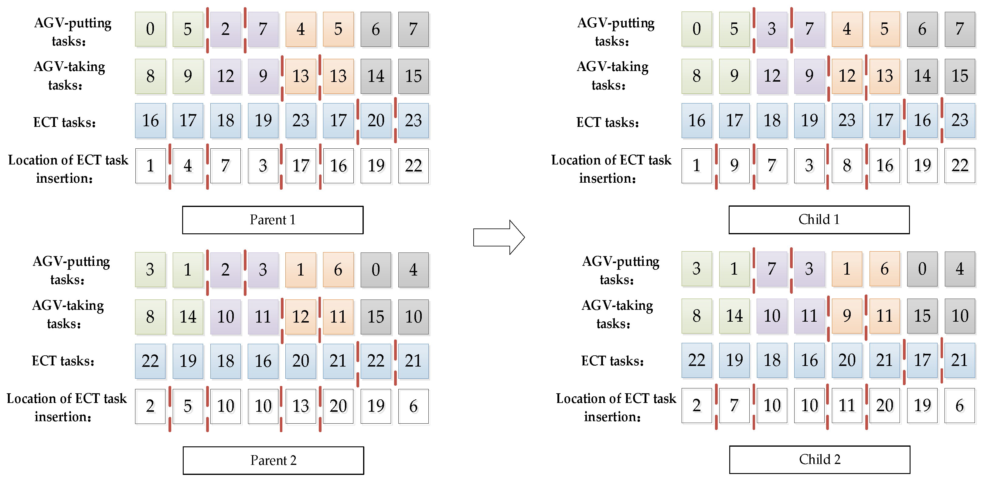
4.3.1. Cross the Task Sequence

The crossover means that the parent task order to be crossed is selected according to the crossover probability. The crossover probabilities for each layer are obtained by adaptive adjustment. A partial crossover is applied to the selected task order. Two crossover points are randomly selected for each chromosome layer, which form a crossover fragment and are crossed in the same layer. The crossover process is shown in Figure 8.

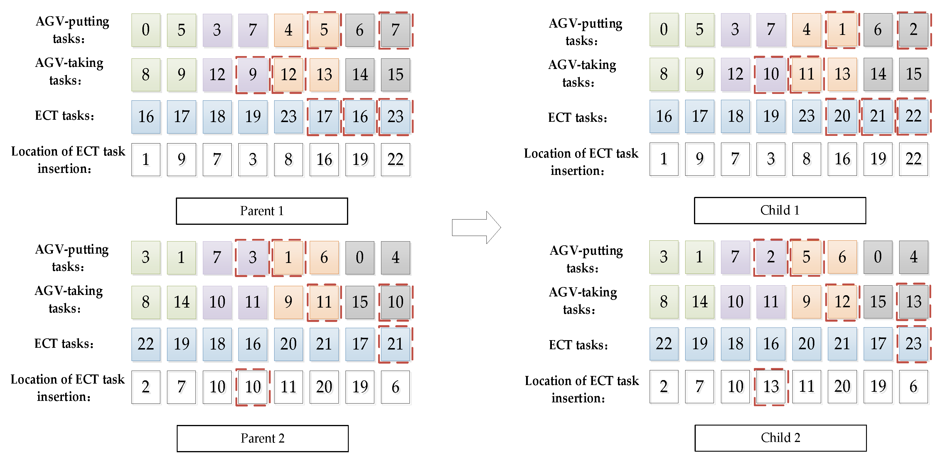
4.3.2. Mutate the Task Sequence

The mutation means that the parent task order to be crossed is selected according to the mutation probability. The mutation probabilities for each stratum are obtained by adaptive adjustment. One to three layers of chromosomes were randomly selected for one task, and the fourth layers of chromosomes were randomly selected for two tasks. The selected tasks were all mutated within the allowed range. The mutation process is shown in Figure 9.

4.4. Repair the Task Sequence

As the new task sequence obtained after crossover or mutation may have duplicated or missing tasks, the repair operation checks the sequence of tasks obtained after crossover and mutation, eliminating duplicate tasks and completing missing tasks. The repair process is shown in Figure 10.

5. Simulation Experiments and Analysis

This chapter first compares the proposed ACGA algorithm with the adaptive genetic algorithms (AGA) [49] and the GA [36] through a small-scale arithmetic example to demonstrate the correctness and practicality of the AA algorithm for solving the present model. Secondly, a sensitivity analysis of the critical factors of the problem is carried out in solving the large-scale arithmetic case to investigate the reasonable allocation of the amount of equipment under the U-shaped ACT.

5.1. Parameter Settings

(1)

Define 4–500 container tasks as small-scale problems and problems above 500 containers as large-scale problems.

(2)

The number of QCs is one to three, the number of AGVs is two to fifty, the number of blocks is two to ten, and the number of ECTs reaches twenty every hour and the arrival times obey a uniform distribution.

(3)

The block and position to be taken or put and the operation type of the ECT are all randomly generated.

(4)

Through multiple experiments by controlling variables, in this paper the maximum number of iterations is set to 20–800 (depending on the number of tasks), the population size is 80, and the initial probabilities of crossover and mutation are set to 0.7 and 0.3, respectively.

(5)

The experiments are implemented in MATLAB 2016a, and all simulations are performed on a computer with Intel Core TM i5 CPU 2.1 GHz and 64 GB RAM under a Windows operating system.

(6)

In the U-shaped ACT, the width of the horizontal transport area is 80 m. There are 99 bays and nine rows in a block. The containers are 12 m long and 2.5 m wide. The DCRC’s gantry and spreader move at a speed of 1 m/s, and the AGV travels at 4m/s. The specific parameters of the ACT are shown in

Table 1. ACT parameters.

Parameters	Numerical Values
Width of horizontal transportation area	80 m
Bay number in block	80
Row number in block	9
Container length	12 m
Container width	2.5 m
Moving speed of DCRC gantry	1 m/s
Moving speed of DCRC spreader	1 m/s
Driving speed of AGV	4 m/s

.

5.2. Results and Algorithm Comparison for Small-Sized Problems

This section examines the feasibility of the model and algorithm in small-scale experiments. Different example sizes are compared, and the performance of the proposed ACGA is analyzed in terms of the OFV, i.e., the total running time of all DCRCs and the required computation time (CPUT).

Table 2. Comparison table of small-scale problems.

No.	Containers	AGVs/DCRCs	ACGA		AGA				GA
			CPUT (s)	OFV (s)	CPUT (s)	OFV (s)	Gap Rate (%)		CPUT (s)	OFV (s)	Gap Rate (%)
							CPUT	OFV			CPUT	OFV
1	20	2/2	1.28	1129	1.27	1287	−0.72	12.28	1.29	1343	0.78	15.96
2	20	2/4	1.58	2918	1.57	3383	−0.60	13.75	1.54	3502	−2.60	16.66
3	20	4/2	1.69	1031	1.66	1199	−1.59	13.99	1.73	1316	2.31	21.67
4	30	5/5	2.35	4698	2.27	5623	−3.55	16.45	2.49	5546	5.62	15.30
5	30	10/5	2.63	4204	2.51	5047	−4.70	16.70	2.69	5206	5.73	19.25
6	30	2/2	1.74	2025	1.68	2376	−3.47	14.78	1.9	2433	8.42	16.75
7	40	4/2	2.13	3305	2.04	3942	−4.20	16.16	2.36	3836	9.75	13.85
8	40	4/4	2.74	5246	2.62	6317	−4.44	16.95	3.11	6347	11.90	17.35
9	50	8/6	3.49	9315	3.32	10,969	−5.18	15.08	3.88	11,115	10.05	16.19
10	50	9/5	2.90	7324	2.75	8658	−5.27	15.41	3.31	8795	12.39	16.70

records the results of the ACGA, GA, and AGA for the case of one QC, varying the number of containers from 20 to 50 and the number of AGVs from two to ten, respectively. Where “Containers” indicate the number of containers at the QC for each test, “AGVs/DCRCs” indicates the number of AGVs and DCRCs used, “CPUT(s)” indicates the time taken for the calculation, and “OFV(s)” indicates the shortest running time of the DCRC for each calculation. The experimental results in Table 2 show that, in terms of CPUT, all three algorithms increase as the problem size increases. The ACGA takes slightly more time than the AGA and is significantly better than the GA. When there were 50 container tasks, the difference between the ACGA and the AGA was about 5%, and the performance improvement with the GA was about 12%. In terms of minimum total running time, the GA, the AGA and the ACGA increase with the number of containers. However, the advantage of the ACGA is demonstrated. The minimum total runtime with the ACGA improves by approximately 15% compared to the GA and the AGA.

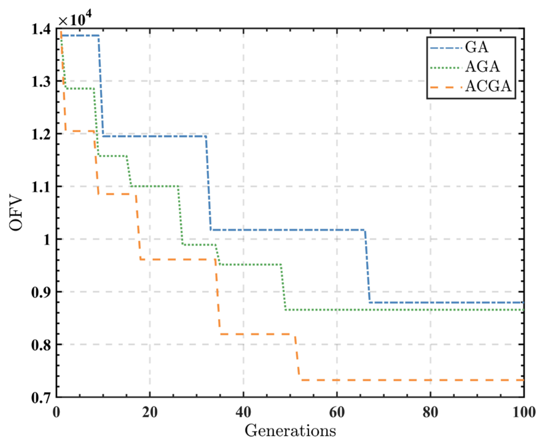
Figure 11 shows the convergence effect of Example 10. The blue line shows the convergence curve of the GA, the green line shows the convergence curve of the AGA, and the orange line shows the convergence curve of the ACGA. As can be seen from the graph, the ACGA and the AGA converge at around 50 generations, both converging faster than the GA, at around 70 generations. At the same time, the ACGA has a significantly lower DCRC total running time and better solution results. The experimental results show that the ACGA can find near-optimal solutions in a short time and has better global search capability. Therefore, the ACGA is used next in solving large-scale algorithms.

5.3. Results and Analysis for Large-Sized Problems

This section examines the impact of different equipment ratios on a large-scale task.

Table 3. Calculation example of 1 QC.

DCRCs-AGVs	OFV(s)	CPUT(s)	DCRCs-AGVs	OFV(s)	CPUT(s)	DCRCs-AGVs	OFV(s)	CPUT(s)	DCRCs-AGVs	OFV(s)	CPUT(s)	DCRCs-AGVs	OFV(s)	CPUT(s)
2–5	81,437	10.61	3–45	77,369	17.76	5–35	83,845	18.88	7–25	98,135	22.45	9–15	117,514	22.86
2–10	70,641	14.08	3–50	77,372	18.98	5–40	84,128	19.18	7–30	94,163	24.08	9–20	113,673	23.37
2–15	71,087	15.31	4–5	89,359	14.08	5–45	84,088	19.59	7–35	90,694	24.59	9–25	108,831	24.49
2–20	71,196	16.84	4–10	85,068	14.18	5–50	84,019	20.92	7–40	91,394	24.69	9–30	105,287	27.35
2–25	70,967	15.51	4–15	81,336	15.20	6–5	102,691	20.20	7–45	91,215	25.71	9–35	104,370	29.08
2–30	71,095	16.53	4–20	79,421	16.12	6–10	99,994	21.43	7–50	91,271	27.14	9–40	101,227	29.18
2–35	70,959	17.24	4–25	79,772	13.47	6–15	96,735	19.90	8–5	115,317	20.51	9–45	98,227	30.10
2–40	71,173	17.86	4–30	79,922	15.71	6–20	93,679	21.02	8–10	111,492	22.65	9–50	98,800	31.12
2–45	70,193	17.45	4–35	79,944	15.61	6–25	90,243	21.53	8–15	108,638	24.29	10–5	129,741	25.10
2–50	71,400	18.37	4–40	80,160	17.45	6–30	87,068	24.18	8–20	106,512	23.57	10–10	126,531	28.37
3–5	84,375	13.16	4–45	80,827	18.57	6–35	87,141	22.45	8–25	103,965	24.18	10–15	123,334	29.69
3–10	80,296	14.18	4–50	80,172	19.59	6–40	87,155	22.04	8–30	99,803	26.43	10–20	120,691	26.94
3–15	76,367	13.57	5–5	98,897	20.31	6–45	87,927	22.65	8–35	97,010	25.41	10–25	117,998	30.31
3–20	77,177	15.00	5–10	95,671	19.08	6–50	88,119	23.47	8–40	94,945	25.10	10–30	115,575	25.82
3–25	77,293	13.57	5–15	90,630	21.73	7–5	112,536	20.31	8–45	94,976	26.63	10–35	111,534	28.88
3–30	77,331	16.12	5–20	87,074	18.27	7–10	109,049	20.31	8–50	94,862	29.29	10–40	107,767	28.57
3–35	76,464	16.73	5–25	83,949	17.86	7–15	105,849	24.49	9–5	122,217	21.02	10–45	104,866	29.39
3–40	76,553	17.24	5–30	84,268	18.27	7–20	101,038	23.06	9–10	120,147	21.94	10–50	101,849	30.20

,

Table 4. Calculation example of 2 QCs.

DCRCs-AGVs	OFV(s)	CPUT(s)	DCRCs-AGVs	OFV(s)	CPUT(s)	DCRCs-AGVs	OFV(s)	CPUT(s)	DCRCs-AGVs	OFV(s)	CPUT(s)	DCRCs-AGVs	OFV(s)	CPUT(s)
2–5	77,897	12.37	3–45	57,782	20.39	5–35	51,217	20.26	7–25	68,291	20.26	9–15	96,756	24.08
2–10	61,974	13.03	3–50	57,571	21.58	5–40	51,862	19.74	7–30	65,047	20.00	9–20	94,556	26.84
2–15	62,381	13.82	4–5	72,956	13.95	5–45	51,668	20.79	7–35	62,878	21.84	9–25	90,110	28.42
2–20	62,308	12.89	4–10	66,817	13.95	5–50	51,448	21.05	7–40	62,915	23.03	9–30	87,274	29.21
2–25	62,543	14.08	4–15	58,604	15.53	6–5	62,632	17.11	7–45	62,505	24.87	9–35	83,224	30.26
2–30	61,981	15.13	4–20	50,990	14.21	6–10	60,355	18.95	7–50	61,760	25.79	9–40	80,114	30.39
2–35	62,357	14.21	4–25	51,098	15.00	6–15	59,435	19.61	8–5	99,272	21.45	9–45	76,563	31.97
2–40	63,049	15.00	4–30	50,629	13.95	6–20	57,463	19.61	8–10	96,875	23.16	9–50	76,901	33.42
2–45	62,654	15.79	4–35	50,321	16.71	6–25	56,849	18.16	8–15	92,156	23.16	10–5	117,498	24.08
2–50	62,688	16.58	4–40	50,574	16.32	6–30	55,626	19.61	8–20	89,666	25.66	10–10	113,019	26.18
3–5	73,847	13.55	4–45	50,639	17.89	6–35	56,032	19.87	8–25	83,810	24.21	10–15	108,703	27.24
3–10	63,594	13.82	4–50	51,760	19.08	6–40	56,039	20.13	8–30	79,476	26.32	10–20	105,409	28.16
3–15	57,578	13.03	5–5	61,748	16.58	6–45	55,792	21.32	8–35	74,576	27.63	10–25	102,564	29.47
3–20	58,102	14.21	5–10	58,475	16.84	6–50	55,909	22.63	8–40	70,128	28.29	10–30	98,156	32.50
3–25	57,743	15.66	5–15	55,784	17.89	7–5	85,278	18.03	8–45	70,641	30.66	10–35	95,838	33.95
3–30	57,673	17.37	5–20	53,014	17.63	7–10	81,612	18.42	8–50	69,849	32.63	10–40	92,097	34.34
3–35	57,898	19.08	5–25	51,355	17.63	7–15	77,056	19.47	9–5	103,102	23.16	10–45	88,525	34.87
3–40	57,602	20.92	5–30	51,971	18.55	7–20	72,028	18.55	9–10	99,831	23.68	10–50	84,330	36.05

and

Table 5. Calculation example of 3 QCs.

DCRCs-AGVs	OFV(s)	CPUT(s)	DCRCs-AGVs	OFV(s)	CPUT(s)	DCRCs-AGVs	OFV(s)	CPUT(s)	DCRCs-AGVs	OFV(s)	CPUT(s)	DCRCs-AGVs	OFV(s)	CPUT(s)
2–5	58,467	18.57	3–45	51,769	31.53	5–35	40,283	27.76	7–25	47,874	31.23	9–15	70,497	37.36
2–10	54,852	19.80	3–50	52,043	33.67	5–40	40,579	28.98	7–30	44,406	30.88	9–20	67,450	39.93
2–15	54,966	26.33	4–5	56,334	20.61	5–45	40,051	31.53	7–35	42,727	36.20	9–25	63,971	44.37
2–20	54,914	20.92	4–10	54,639	21.53	5–50	41,128	34.69	7–40	43,246	39.04	9–30	59,847	49.51
2–25	54,827	19.08	4–15	50,224	28.88	6–5	49,512	31.33	7–45	43,264	39.75	9–35	56,566	50.40
2–30	54,869	21.94	4–20	46,184	22.76	6–10	45,777	30.51	7–50	42,654	39.31	9–40	52,259	46.41
2–35	54,773	20.92	4–25	46,922	25.10	6–15	41,263	23.78	8–5	69,864	33.19	9–45	49,608	52.35
2–40	54,828	25.00	4–30	47,520	20.00	6–20	39,835	33.78	8–10	65,199	35.30	9–50	49,713	52.00
2–45	54,883	26.73	4–35	46,011	26.12	6–25	38,032	34.59	8–15	63,669	36.11	10–5	79,906	38.65
2–50	54,796	29.18	4–40	45,934	25.41	6–30	37,734	35.92	8–20	61,748	35.94	10–10	77,083	41.42
3–5	57,723	18.67	4–45	46,639	27.65	6–35	37,932	38.57	8–25	57,940	41.88	10–15	74,329	41.74
3–10	53,654	19.90	4–50	46,007	30.82	6–40	38,365	39.29	8–30	53,056	41.17	10–20	71,833	43.76
3–15	51,246	24.29	5–5	50,231	25.41	6–45	37,486	34.08	8–35	50,825	43.48	10–25	68,519	45.54
3–20	51,303	20.31	5–10	48,678	20.71	6–50	37,593	38.27	8–40	47,064	44.19	10–30	64,965	48.87
3–25	51,271	28.78	5–15	44,377	36.53	7–5	62,884	27.60	8–45	47,748	39.75	10–35	60,289	51.80
3–30	50,993	25.61	5–20	41,747	27.55	7–10	59,611	28.66	8–50	47,649	40.46	10–40	58,568	55.05
3–35	51,096	24.80	5–25	39,495	37.96	7–15	55,589	32.83	9–5	75,614	35.47	10–45	54,050	56.22
3–40	51,244	27.45	5–30	40,036	29.29	7–20	51,165	29.90	9–10	72,052	35.76	10–50	51,630	59.09

record the results of varying the number of AGVs from five to fifty and the number of DCRCs from two to ten when using one, two, and three QCs, respectively. Figure 12, Figure 13, Figure 14, Figure 15, Figure 16 and Figure 17 are all plotted from the data in Table 3, Table 4 and Table 5.

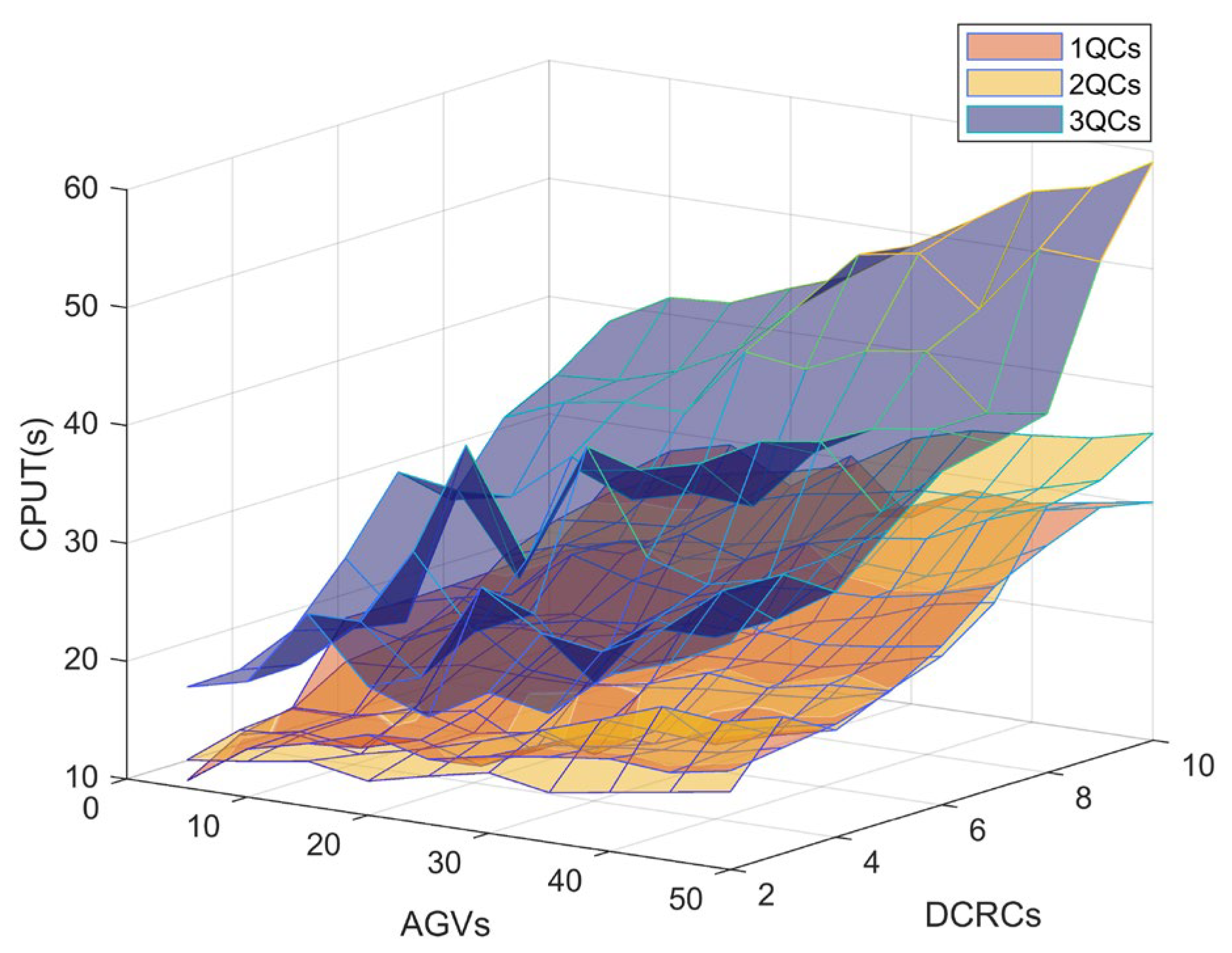
Figure 12 is plotted from the CPUT(s) in Table 3, Table 4 and Table 5. The aim is to analyze the effect of the number of QCs on the required calculation time. As can be seen from the figure, the images are divided into three layers corresponding to the computation time using one to three QCs, respectively. The computation time for the case using one QC is distributed at the bottom of the image and ranges from 10.61 s to 30.31 s. The computation time for the case using three QCs is distributed at the top of the graph and ranges from 18.57 s to 59.09 s. This means that the complexity of the case and the computation time increase with the number of QCs.

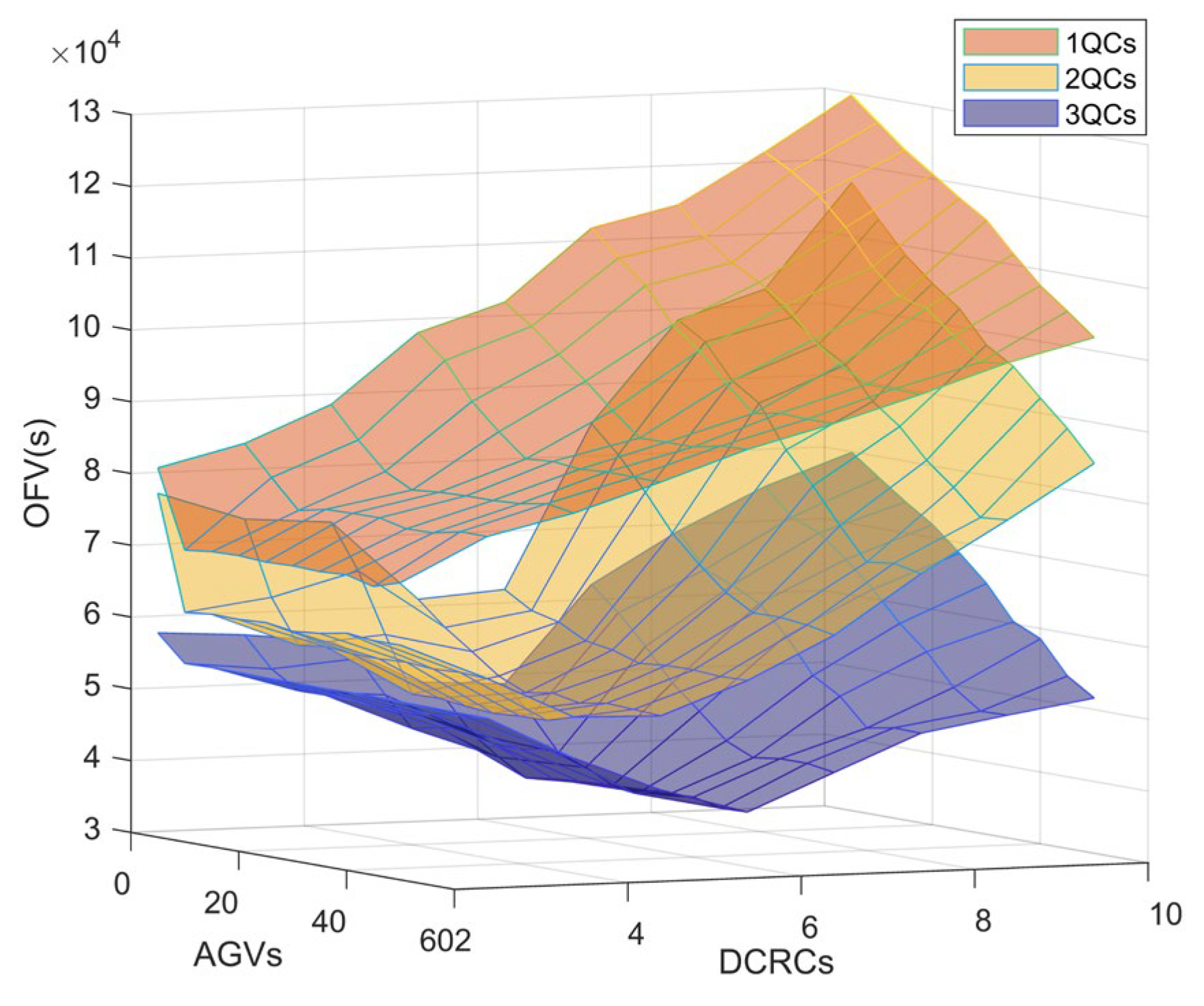
Figure 13 is plotted from the OFV(s) in Table 3, Table 4 and Table 5. The aim is to analyze the effect of the number of QCs on the total running time of all DCRCs. It can be seen that the image is divided into three layers according to the number of QCs. The uppermost layer is the total DCRC running time for one QC, ranging from 70,193 to 129,741 s. The bottom layer is the total DCRC running time for three QCs, which ranges from 39,495 s to 72,052 s. It can be concluded that the higher the number of QCs, the lower the total running time of the DCRC.

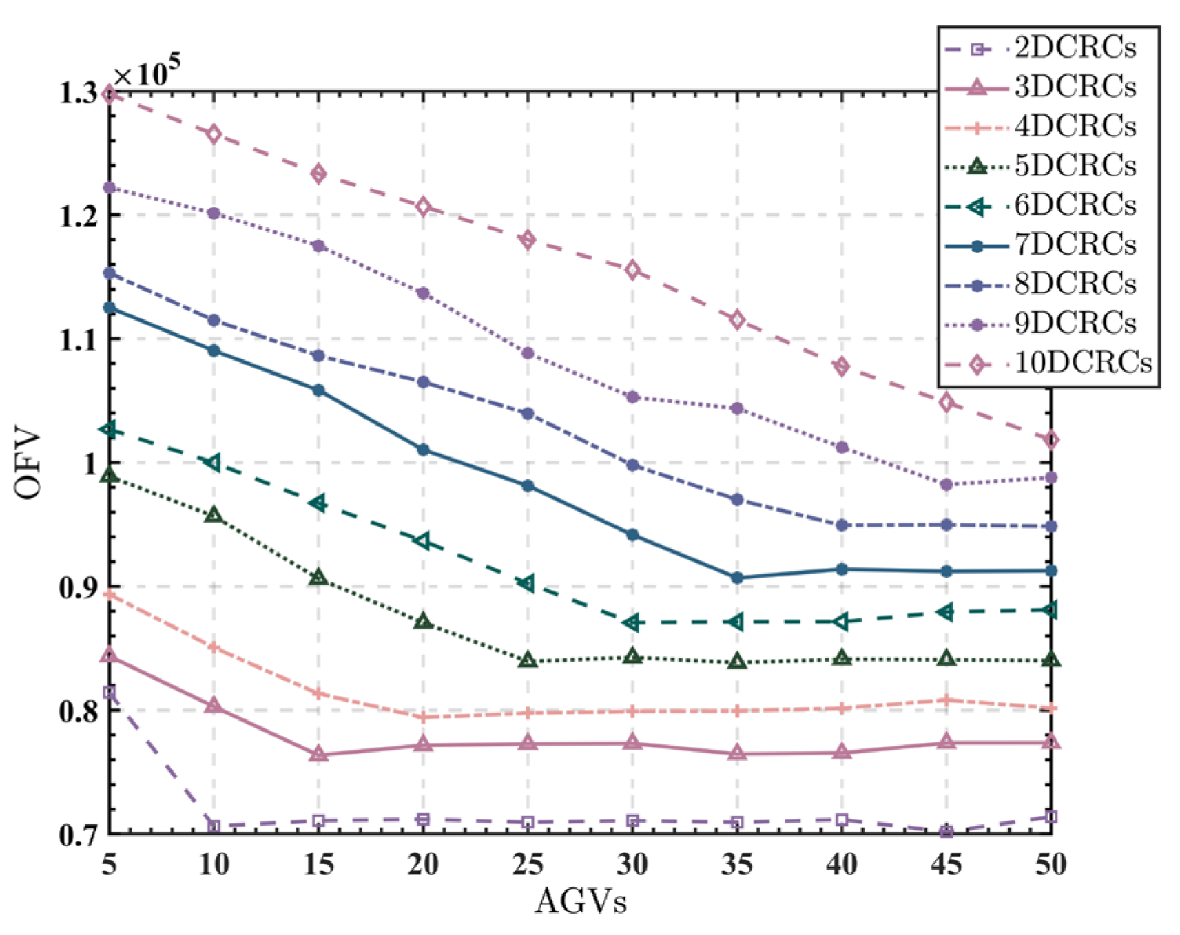
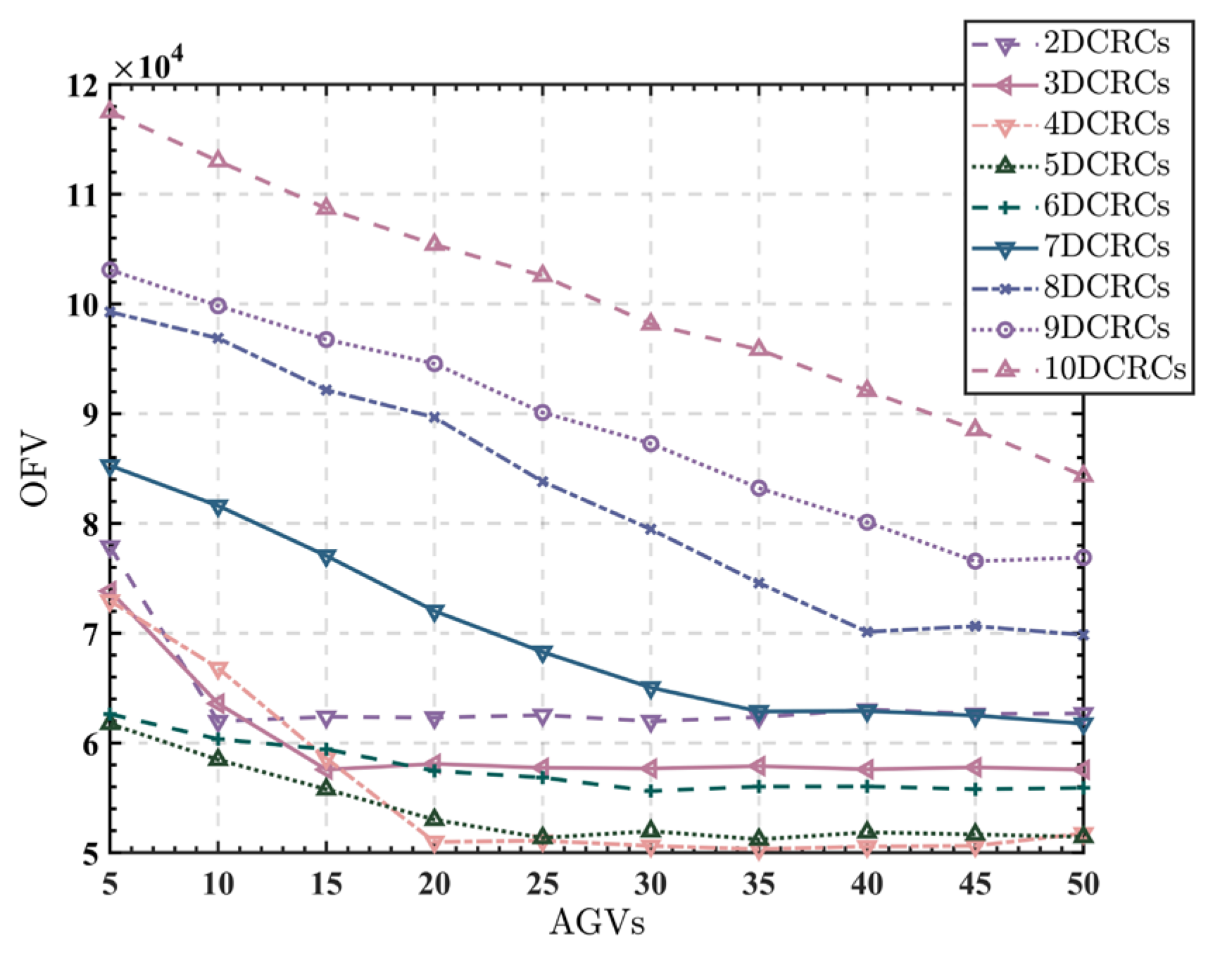
Figure 14, Figure 15 and Figure 16 show the effect of varying the number of DCRCs and AGVs on the total running time of the DCRC at different numbers of QCs. The horizontal coordinate is the number of AGVs, and the vertical coordinate is the OFV. Lines with different colors correspond to the use of different numbers of DCRCs.

Allocating the correct number of DCRCs for the vessels is one of the issues that must be considered by the terminal staff, which will directly affect the overall operating costs and efficiency. As shown in Figure 14, the total running time using two DCRCs is located at the bottom of the diagram when one QC is used. As the number of DCRCs increases, their total running time gradually increases until it reaches a maximum with 10 DCRCs. The case of using two QCs is shown in Figure 15. When the number of DCRCs is increased, the total running time of the DCRCs first decreases—the line corresponding to using four DCRCs is at the bottom of Figure 15, where the result is optimal. Then, as the number of DCRCs increases, the total running time of the DCRC increases rather than decreases. The same situation occurs when using three QCs, as shown in Figure 16. The total running time of the DCRC first decreases as the number of DCRCs increases, until it reaches a minimum when six DCRCs are used, and then gradually increases. It is worth noting that the shortest total running time of the double cantilever rail cranes is achieved when the number of DCRCs and QCs is 2:1 rather than more.

The AGV is an essential part of the transport chain on the quay. If the number of AGVs is too small, it cannot meet the working needs of the horizontal transportation of the quay, and if the number of AGVs is too large, it will cause a problem of wasted resources. As can be seen from Figure 14, Figure 15 and Figure 16, the total running time of the DCRC gradually decreases as the number of AGVs increases, but the two are not exactly positively correlated. When the number of QCs is fixed, the minimum total running time of the DCRC is always generated around a specific number of AGVs and then plateaus. For example, when the number of QCs is one, the shortest total running time of the DCRC is generated around the AGV number of 10. When the number of QCs is two, the shortest total running time of the DCRC is generated at around 20 for the AGV. When the number of QCs is three, the shortest total running time of the DCRC is generated at around 30 for the AGV. It can be seen that the number of AGVs and QCs should be kept at around 10:1, when the total running time of the DCRC is the shortest and the number of AGVs required is the least.

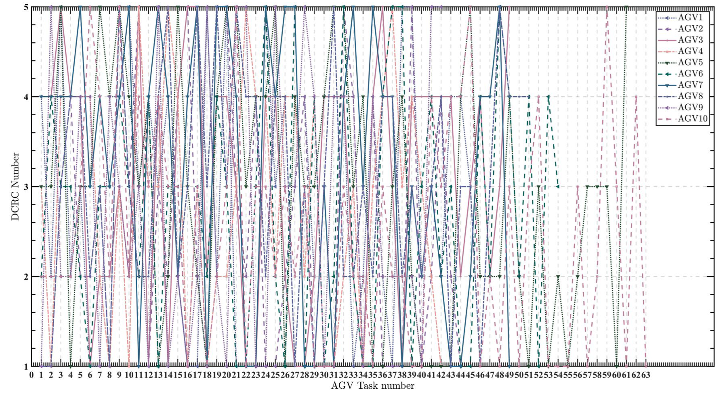
Figure 17 shows the optimal scheduling scheme for 500 container tasks using one QC, ten AGVs, and five DCRCs. The horizontal axis represents the tasks of the AGVs, and the vertical axis represents the corresponding DCRCs. This figure is a concrete manifestation of the case study in our paper, which visually demonstrates the tasks of each device and further proves the feasibility of our model and algorithm.

The above analysis shows that the calculation time required for scheduling increases with the number of tasks, QCs and DCRCs. The total running time of the DCRC generally decreases as the number of QCs, DCRCs, and AGVs increases. However, when the number of QCs is fixed, the number of DCRCs and AGVs is not as high as it could be. When the number of both reaches a certain level, adding more equipment will not effectively reduce the total running time of the DCRC but may increase it. According to the above analysis, we can conclude that, in the U-shaped ACT loading and unloading process, a QC equipped with two DCRCs and ten AGVs will have a total running time of DCRCs. At the same time, the impact of the change in the number of QCs and DCRCs on the total running time of the DCRCs is greater than the impact of the change in the number of AGVs. Therefore, the allocation of resources for QCs and DCRCs should be considered first in the actual operation of U-shaped ACTs.

6. Conclusions

To improve the operational efficiency of the U-shaped ACT and to fit its actual operational characteristics, this paper first optimizes the working process of U-shaped ACTs. In U-shaped ACTs, the movement of the DCRC during loading and unloading is described in more detail by grouping the 16 working conditions into four operating modes based on how the DCRC works. Secondly, to minimize the total running time of all DCRCs, a refined collaborative dispatching model for AGVs and DCRCs, considering the entry of ECTs into the yard, was developed based on these four operating modes. This improves the accuracy of the modeling. The model is then solved using the ACGA to verify the model’s correctness and the algorithm’s practicality. Finally, experimental simulations were carried out to derive the optimum ratio of each equipment in different environments. The results show that, in the U-shaped ACT, the optimal ratio of the QC to the DCRC and the AGV is 1:2 and 1:10, respectively, where the total running time of DCRCs is the shortest. Simultaneously, the number of QCs and DCRCs has a more significant impact on terminal efficiency than the AGVs, and priority should be given to the allocation of both. This addresses the realities of U-shaped ACTs, and provides a reference for the construction.

However, the problem of multi-device scheduling in U-shaped ACTs is a highly complex one, and this study still has several shortcomings that need to be addressed in future research to improve and refine its findings.

Firstly, this study focused solely on efficiency-oriented collaborative scheduling, neglecting to consider energy consumption issues. However, energy consumption plays a vital role in practical applications, and it is crucial to consider optimizing device collaborative scheduling to strike a balance between economic and environmental factors.

Secondly, this study did not include the QC, which is another critical device with complex coupling relationships with AGVs. Future research should, therefore, incorporate the QC into the scheduling to achieve more comprehensive and refined results.

Thirdly, the mutual interference between multiple YCs has not been thoroughly investigated, which may significantly affect the overall efficiency of the ACT. As such, this area should be explored in more depth to achieve more efficient and stable ACT operations.

Furthermore, while this study primarily focuses on scheduling issues, it fails to address the path planning of AGVs, which is a vital component that requires the comprehensive consideration of various factors, such as time, distance, vehicle speed, and safety, to achieve optimal results.

Lastly, the study did not consider the charging issue of AGVs, which is essential in practical operations. To achieve a long-term and efficient operation of AGVs, the charging issue should also be considered while optimizing scheduling. It is, therefore, suggested that future research should include these factors in their modeling efforts to develop more realistic and effective solutions.

References

- Yang, Y.; Zhong, M.; Dessouky, Y.; Postolache, O. An integrated scheduling method for AGV routing in automated container terminals. Comput. Ind. Eng. 2018, 126, 482–493. [Google Scholar] [CrossRef]
- Yu, H.; Huang, M.; He, J.; Tan, C. The clustering strategy for stacks allocation in automated container terminals. Marit. Policy Manag. 2022, 1–16. [Google Scholar] [CrossRef]
- Bierwirth, C.; Meisel, F. A survey of berth allocation and quay crane scheduling problems in container terminals. Eur. J. Oper. Res. 2010, 202, 615–627. [Google Scholar] [CrossRef]
- Wang, N.; Chang, D.; Shi, X.; Yuan, J.; Gao, Y. Analysis and design of typical automated container terminals layout considering carbon emissions. Sustain 2019, 11, 2957. [Google Scholar] [CrossRef] [Green Version]
- Lee, B.K.; Lee, L.H.; Chew, E.P. Analysis on high throughput layout of container yards. Int. J. Prod. Res. 2018, 56, 5345–5364. [Google Scholar] [CrossRef]
- Liu, C.I.; Jula, H.; Vukadinovic, K.; Ioannou, P. Automated guided vehicle system for two container yard layouts. Transp. Res. Part C Emerg. Technol. 2004, 12, 349–368. [Google Scholar] [CrossRef]
- Roy, D.; Gupta, A.; Parhi, S.; De Koster, M.B.M. Optimal Stack Layout in a Sea Container Terminal with Automated Lifting Vehicles. SSRN Electron. J. 2017, 55, 3747–3765. [Google Scholar] [CrossRef] [Green Version]
- Xu, B.; Jie, D.; Li, J.; Yang, Y.; Wen, F.; Song, H. Integrated scheduling optimization of U-shaped automated container terminal under loading and unloading mode. Comput. Ind. Eng. 2021, 162, 107695. [Google Scholar] [CrossRef]
- Gharehgozli, A.; Zaerpour, N.; de Koster, R. Container terminal layout design: Transition and future. Marit. Econ. Logist. 2020, 22, 610–639. [Google Scholar] [CrossRef]
- Li, J.; Yang, J.; Xu, B.; Yang, Y.; Wen, F.; Song, H. Hybrid scheduling for multi-equipment at u-shape trafficked automated terminal based on chaos particle swarm optimization. J. Mar. Sci. Eng. 2021, 9, 1080. [Google Scholar] [CrossRef]
- Niu, Y.; Yu, F.; Yao, H.; Yang, Y. Multi-equipment coordinated scheduling strategy of U-shaped automated container terminal considering energy consumption. Comput. Ind. Eng. 2022, 174, 108804. [Google Scholar] [CrossRef]
- He, J.; Chang, D.; Mi, W.; Yan, W. A hybrid parallel genetic algorithm for yard crane scheduling. Transp. Res. Part E Logist. Transp. Rev. 2010, 46, 136–155. [Google Scholar] [CrossRef]
- Chang, D.; Jiang, Z.; Yan, W.; He, J. Developing a dynamic rolling-horizon decision strategy for yard crane scheduling. Adv. Eng. Inform. 2011, 25, 485–494. [Google Scholar] [CrossRef]
- He, J.; Huang, Y.; Yan, W. Yard crane scheduling in a container terminal for the trade-off between efficiency and energy consumption. Adv. Eng. Inform. 2015, 29, 59–75. [Google Scholar] [CrossRef]
- Tan, C.; He, J.; Yu, H.; Tang, Y. Modelling the problem of yard crane deployment for resource-limited container terminal. Int. J. Ind. Syst. Eng. 2019, 32, 137–169. [Google Scholar] [CrossRef]
- He, J.; Tan, C.; Zhang, Y. Yard crane scheduling problem in a container terminal considering risk caused by uncertainty. Adv. Eng. Inform. 2019, 39, 14–24. [Google Scholar] [CrossRef]
- Liu, W.; Zhu, X.; Wang, L.; Yan, B.; Zhang, X. Optimization Approach for Yard Crane Scheduling Problem with Uncertain Parameters in Container Terminals. J. Adv. Transp. 2021, 2021, 1–15. [Google Scholar] [CrossRef]
- Ng, W.C. Crane scheduling in container yards with inter-crane interference. Eur. J. Oper. Res. 2005, 164, 64–78. [Google Scholar] [CrossRef]
- Wu, Y.; Li, W.; Petering, M.E.; Goh, M.; Souza, R.D. Scheduling multiple yard cranes with crane interference and safety distance requirement. Transp. Sci. 2015, 49, 990–1005. [Google Scholar] [CrossRef] [Green Version]
- Zheng, F.; Man, X.; Chu, F.; Liu, M.; Chu, C. Two yard crane scheduling with dynamic processing time and interference. IEEE Trans. Intell. Transp. Syst. 2018, 19, 3775–3784. [Google Scholar] [CrossRef]
- Fatemi Ghomi, M.S.; Javanshir, H.; Ganji, S.S.; Fatemi Ghomi, S.M.T. Optimisation of yard crane scheduling considering velocity coefficient and preventive maintenance. Int. J. Shipp. Transp. Logist. 2014, 6, 88–108. [Google Scholar] [CrossRef]
- Nossack, J.; Briskorn, D.; Pesch, E. Container dispatching and conflict-free yard crane routing in an automated container terminal. Transp. Sci. 2018, 52, 1059–1076. [Google Scholar] [CrossRef]
- Eilken, A. A decomposition-based approach to the scheduling of identical automated yard cranes at container terminals. J. Sched. 2019, 22, 517–541. [Google Scholar] [CrossRef]
- Kim, K.H.; Lee, K.M.; Hwang, H. A study on multi-ASC scheduling method of automated container terminals based on graph theory. Comput. Ind. Eng. 2019, 129, 404–416. [Google Scholar] [CrossRef]
- Kim, K.H.; Lee, K.M.; Hwang, H. Sequencing delivery and receiving operations for yard cranes in port container terminals. Int. J. Prod. Econ. 2003, 84, 283–292. [Google Scholar] [CrossRef]
- Huang, Y.; Liang, C.; Yang, Y. The optimum route problem by genetic algorithm for loading/unloading of yard crane. Comput. Ind. Eng. 2009, 56, 993–1001. [Google Scholar] [CrossRef]
- Lee, B.K.; Kim, K.H. Comparison and evaluation of various cycle-time models for yard cranes in container terminals. Int. J. Prod. Econ. 2010, 126, 350–360. [Google Scholar] [CrossRef]
- Bhatnagar, R.; Chandra, P.; Goyal, S.K. Models for multi-plant coordination. Eur. J. Oper. Res. 1993, 67, 141–160. [Google Scholar] [CrossRef]
- Chen, X.; He, S.; Zhang, Y.; Tong, L.C.; Shang, P.; Zhou, X. Yard crane and AGV scheduling in automated container terminal: A multi-robot task allocation framework. Transp. Res. Part C Emerg. Technol. 2020, 114, 241–271. [Google Scholar] [CrossRef]
- Zhao, Q.; Ji, S.; Zhao, W.; De, X. A Multilayer Genetic Algorithm for Automated Guided Vehicles and Dual Automated Yard Cranes Coordinated Scheduling. Math. Probl. Eng. 2020, 2020, 1–13. [Google Scholar] [CrossRef]
- Zhang, Q.; Hu, W.; Duan, J.; Qin, J. Cooperative Scheduling of AGV and ASC in Automation Container Terminal Relay Operation Mode. Math. Probl. Eng. 2021, 2021, 1–18. [Google Scholar] [CrossRef]
- Yang, X.M.; Jiang, X.J. Yard Crane Scheduling in the Ground Trolley-Based Automated Container Terminal. Asia-Pac. J. Oper. Res. 2020, 37, 2050007. [Google Scholar] [CrossRef]
- Hsu, H.P.; Tai, H.H.; Wang, C.N.; Chou, C.C. Scheduling of collaborative operations of yard cranes and yard trucks for export containers using hybrid approaches. Adv. Eng. Inform. 2021, 48, 101292. [Google Scholar] [CrossRef]
- Zhou, C.; Lee, B.K.; Li, H. Integrated optimization on yard crane scheduling and vehicle positioning at container yards. Transp. Res. Part E Logist. Transp. Rev. 2020, 138, 101966. [Google Scholar] [CrossRef]
- Roy, D.; de Koster, R. Stochastic modeling of unloading and loading operations at a container terminal using automated lifting vehicles. Eur. J. Oper. Res. 2018, 266, 895–910. [Google Scholar] [CrossRef] [Green Version]
- Li, H.; Peng, J.; Wang, X.; Wan, J. Integrated Resource Assignment and Scheduling Optimization with Limited Critical Equipment Constraints at an Automated Container Terminal. IEEE Trans. Intell. Transp. Syst. 2021, 22, 7607–7618. [Google Scholar] [CrossRef]
- Lu, Y.; Le, M. The integrated optimization of container terminal scheduling with uncertain factors. Comput. Ind. Eng. 2014, 75, 209–216. [Google Scholar] [CrossRef]
- He, J.; Huang, Y.; Yan, W.; Wang, S. Integrated internal truck, yard crane and quay crane scheduling in a container terminal considering energy consumption. Expert Syst. Appl. 2015, 42, 2464–2487. [Google Scholar] [CrossRef]
- Ahmed, E.; El-Abbasy, M.S.; Zayed, T.; Alfalah, G.; Alkass, S. Synchronized scheduling model for container terminals using simulated double-cycling strategy. Comput. Ind. Eng. 2021, 154, 107118. [Google Scholar] [CrossRef]
- Zhang, X.; Zeng, Q.; Yang, Z. Optimization of truck appointments in container terminals. Marit. Econ. Logist. 2019, 21, 125–145. [Google Scholar] [CrossRef]
- Chen, X.; Wu, X.; Prasad, D.K.; Wu, B.; Postolache, O.; Yang, Y. Pixel-Wise Ship Identification From Maritime Images via a Semantic Segmentation Model. IEEE Sens. J. 2022, 22, 18180–18191. [Google Scholar] [CrossRef]
- Chen, X.; Liu, S.; Liu, R.W.; Wu, H.; Han, B.; Zhao, J. Quantifying Arctic oil spilling event risk by integrating an analytic network process and a fuzzy comprehensive evaluation model. Ocean Coast. Manag. 2022, 228, 106326. [Google Scholar] [CrossRef]
- Li, X.; Peng, Y.; Huang, J.; Wang, W.; Song, X. Simulation study on terminal layout in automated container terminals from efficiency, economic and environment perspectives. Ocean Coast. Manag. 2021, 213, 105882. [Google Scholar] [CrossRef]
- Lau, H.Y.; Zhao, Y. Integrated scheduling of handling equipment at automated container terminals. Int. J. Prod. Econ. 2008, 112, 665–682. [Google Scholar] [CrossRef]
- Kaveshgar, N.; Huynh, N.; Rahimian, S.K. An efficient genetic algorithm for solving the quay crane scheduling problem. Expert Syst. Appl. 2012, 39, 13108–13117. [Google Scholar] [CrossRef]
- Deng, Z.; Fan, J.; Shi, Y.; Shen, W. A Coevolutionary algorithm for cooperative platoon formation of connected and automated vehicles. IEEE Trans. Veh. Technol. 2022, 71, 12461–12474. [Google Scholar] [CrossRef]
- Valenzuela-Alcaraz, V.M.; Cosio-Leon, M.A.; Romero-Ocaño, A.D.; Brizuela, C.A. A cooperative coevolutionary algorithm approach to the no-wait job shop scheduling problem. Expert Syst. Appl. 2022, 194, 116498. [Google Scholar] [CrossRef]
- Zhang, X.; Ma, Z.; Ding, B.; Fang, W.; Qian, P. A coevolutionary algorithm based on the auxiliary population for constrained large-scale multi-objective supply chain network. Math. Biosci. Eng. 2022, 19, 271–286. [Google Scholar] [CrossRef] [PubMed]
- So, C.; Ho, I.M.; Chae, J.S.; Hong, K.H. PWR core loading pattern optimization with adaptive genetic algorithm. Ann. Nucl. energy 2021, 159, 108331. [Google Scholar] [CrossRef]