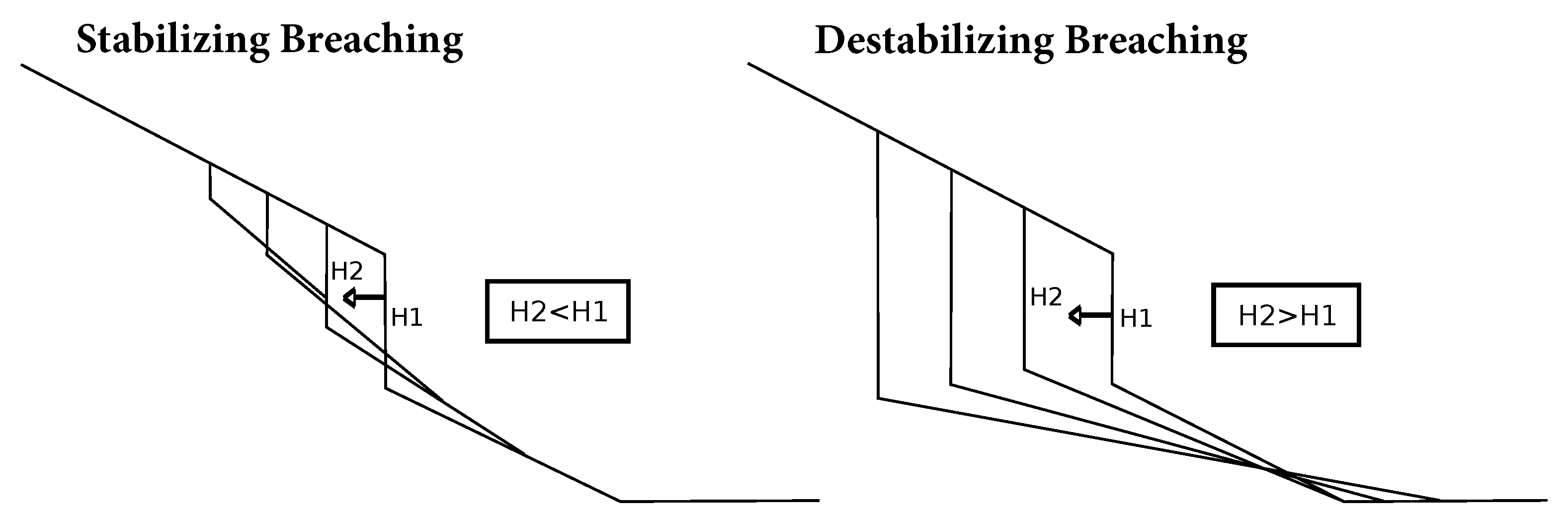
Stabilizing and Destabilizing Breaching Flow Slides

Abstract

As a result of the dilation of soil matrix, dense submarine sand slopes can temporarily be steeper than the natural angle of repose. These slopes gradually fail by the detachment of individual grains and intermittent collapses of small coherent sand wedges. The key question is whether steep disturbances in a submarine slope grow in size (destabilizing breaching) or gradually diminish (stabilizing breaching) and thereby limit the overall slope failure and resulting damage. The ability to predict whether the breaching failure is stabilizing or destabilizing is also crucial for the assessment of safety of submarine infrastructure and hydraulic structures located along rivers, lakes, and coasts. Through a set of large-scale laboratory experiments, we investigate the validity of an existing criterion to determine the failure mode of breaching (i.e., stabilizing or destabilizing). Both modes were observed in these experiments, providing a unique set of data for analysis. It is concluded that the existing method has limited forecasting power. This was quantified using the mean absolute percentage error, which was found to be 92%. The reasons behind this large discrepancy are discussed. Given the complexity of the underlying geotechnical and hydraulic processes, more advanced methodologies are required.

1. Introduction

Subaqueous slope failure is a common problem in the fields of geotechnical, hydraulic, and dredging engineering, posing a serious threat to underwater infrastructure and flood defence structures along rivers, lakes, and coasts. One of the possible failure mechanisms is ‘flow slide’, which occurs when the sediment deposit loses its stability and runs downslope, forming a gentler slope than the initial one [1]. During flow slides, the sediment is transported as a sediment–water mixture, which behaves as a viscous fluid [2]. Two end members of flow slides are distinguished in the literature: liquefaction flow slides and breaching flow slides. The former occurs in loosely-packed sand, which shows a contractive behaviour under shear forces; the soil structure collapses abruptly and a large amount of the soil body flows downslope. The latter, on the other hand, does not occur as an abrupt collapse. Rather, sand grains peel off particle by particle, generating a turbidity current propagating over the slope surface (or ‘breach face’) [3,4,5].

Unlike static liquefaction, breaching is mostly encountered in densely-packed sand, which dilates under shear forces [3,6]. Dilative sand undergoes an increase in pore volume under shear deformation, leading to the generation of a negative pore pressure, which substantially retards the sand erosion process [7]. An inward hydraulic gradient is generated, as a result of the pressure difference, forcing the ambient water to seep into the pores, dissipating the negative pressure. Consequently, the sand grains located at the sand–water interface destabilize and gradually peel off, almost grain by grain [5,8]. These grains mix and interact with the ambient water, forming a sustained turbidity current travelling along the breach face and subsequently down the slope toe [9].

Breaching-generated turbidity currents are self-accelerating [5]. They induce an additional shear stress on the breach face, thereby picking up more sediment, which makes the turbidity current denser. As a consequence, the current expedites downslope, boosting its erosive capacity and leading to higher erosion rates in the downstream direction. This implies that sediment entrainment and acceleration of the turbidity current are coupled in a positive feedback loop. Next to the grain-by-grain erosion, intermittent collapses of coherent sand wedges, termed surficial slides, have been observed in breaching lab experiments [3,5,10]. The current understanding of the occurrence of surficial slides remains poor [8].

In dredging engineering, breaching is triggered deliberately for sand mining purposes [3]. It should be noted, however, that natural breaching events can also occur. The mechanisms that trigger these events are not yet fully understood. For example, at Amity Point in Queensland, Australia, breaching events continue to be observed without a clear understanding of their triggers [11].

Breaching, both naturally occurring and anthropogenic, can last for several hours, travelling towards nearby or remote shorelines or river banks, posing a major risk [11,12]. Additionally, breaching could cause instabilities during the construction of underwater slopes [6]. Such risky situations could be avoided by developing a good understanding of the spatio-temporal evolution of breaching. In this regard, prior experimental observations showed that two failure modes of breaching can be distinguished [3]: stabilizing and destabilizing (Figure 1). Breaching is regarded as destabilizing when the breach face increases in height over time, resulting in an uncontrolled retrogressive failure of the slope. In contrast, during stabilizing breaching, the height of the breach face decreases over time until it disappears completely.

On the modelling side, a few numerical models for breaching-generated turbidity currents have been proposed in the literature. Most of these numerical investigations were mostly restricted to layer-averaged, one-dimensional models, where several empirical closure relations are required (e.g., [1,4,9]). However, Alhaddad et al. [8] presented 3D large-eddy-resolving numerical simulations, providing deeper insights into the flow structure and hydrodynamics of breaching-generated turbidity currents. Additionally, Van Rhee [6,13] simulated breaching by a two-dimensional computational fluid dynamics code coupled with a bed boundary condition to model sediment erosion and as well as an empirical approach to assess the failure mode of breaching. The latter will be discussed in detail in this study.

This paper presents results of laboratory experiments where we investigate the failure mode of breaching. Several initial conditions were tested, allowing us to observe both stabilizing and destabilizing breaching. Following that, we utilize our experimental measurements to provide the first insights into the validity of the approach used in the literature to assess the failure mode of breaching. Lastly, key future research directions are defined to improve the predictability of breaching mode.

2. Existing Method for Failure Mode Assessment

The mode of a 2D breaching failure can be assessed by a simple geometric argument. Using the schematized slope profile depicted in Figure 2, the following relation can be derived for the spatial change of the breach height, H:

$$\frac{dH}{dx}=\frac{1}{\Delta x}\left(\Delta y_2-\Delta y_1\right)=\frac{\Delta xtan{\beta }_{top}-\Delta xtan{\beta }_{toe}}{\Delta x}=tan{\beta }_{top}-tan{\beta }_{toe},$$

(1)

where ${\beta }_{toe}$ is the angle of the slope at the toe of the breach face and ${\beta }_{top}$ is the angle of the slope at the top of the breach face. It follows that

$$\mathrm{breaching}\mathrm{mode}\mathrm{is}\left\{\begin{array}{cc}\mathrm{stabilizing}\mathrm{if}\hfill & \frac{dH}{dx}<0\hfill \\ \\ \mathrm{destabilizing}\mathrm{if}\hfill & \frac{dH}{dx}>0.\hfill \end{array}\right.$$

(2)

This means that to predict the sign of $dH/dx$ it is essential to estimate the angle of the slope at the toe, ${\beta }_{toe}$. Van Rhee [6] suggests that a first estimate for this slope can be obtained following the findings of the sand fill experiments of Mastbergen et al. [14]. In their study, a constant sand flux, s, was applied via a pipe at the beginning of a flume (32 m × 2.5 m × 0.5 m). At the start of the experiment, the flume was filled with water only. Initially, the sand pile was formed below the pipe until the free surface was reached. In the next phase, the sand body gently migrated in a horizontal direction. After some time, the produced slope angle became constant, while the slope kept migrating horizontally; this situation is shown in Figure 3.

The following empirical relation was proposed for the eventual steady slope angle, ${\beta }_{fill}$ (${}^{°})$:

$$tan{\beta }_{fill}=\frac{1623D_{50}^{0.92}}{s^{0.39}},$$

(3)

where $D_{50}$ (m) is the median sand grain size and s ($\mathrm{kg}/\mathrm{m}/\mathrm{s})$ is the sand flux. It should be realized that the calibration coefficient (1623) is not dimensionless. Assuming that the slope at the toe has enough time to adapt to the sand flux provided by the breach face, it follows that

$${\beta }_{toe}\approx {\beta }_{fill}.$$

(4)

For breaching, the sand flux, s, at the beginning of the toe slope reads [13]:

$$s=v_{breach}H{\rho }_s(1-n_0),$$

(5)

where $v_{breach}$ is the erosion velocity of the breach face, ${\rho }_s$ is the density of the sand particles and $n_0$ is the in situ porosity. The critical value between stabilizing breaching ($dH/dx<0$) and destabilizing breaching ($dH/dx>0$) can be found by setting,

$$0=\frac{dH}{dx}=tan{\beta }_{top}-tan{\beta }_{toe}.$$

(6)

Now it follows that

$$tan{\beta }_{toe}=tan{\beta }_{fill}=\frac{1623D_{50}^{0.92}}{s^{0.39}}=tan{\beta }_{top}.$$

(7)

Substitution of Equation (5) gives the following expression for the critical breach height:

$$H_{crit}={\left(\frac{1623D_{50}^{0.92}}{tan{\beta }_{top}}\right)}^{2.6}\frac{1}{v_{breach}{\rho }_s(1-n_0)}.$$

(8)

If desired, the erosion velocity of the breach face $v_{breach}$ can be calculated [6] as follows:

$$v_{breach}=\frac{1-n_l}{n_l-n_0}{k}_l(1-n_0)\frac{{\rho }_s-{\rho }_w}{{\rho }_w}\frac{sin({\beta }_{breach}-\varphi )}{sin\varphi },$$

(9)

where $\varphi$ (${}^{°}$) is the internal friction angle, ${\beta }_{breach}$ (${}^{°}$) is the slope angle of the breach face, $n_0$ (-) is the in situ porosity of the sand, $n_l$ (-) is the maximum porosity of the sand, $k_l$ ($\mathrm{m}/\mathrm{s}$) is the sand hydraulic conductivity at maximum porosity, ${\rho }_s$ ($\mathrm{kg}/{\mathrm{m}}^3$) is the density of the particles, and ${\rho }_w$ ($\mathrm{kg}/{\mathrm{m}}^3$) is the density of water.

If $H>H_{crit}$, we have destabilizing breaching and if $H<H_{crit}$, we have stabilizing breaching. Figure 4 visualizes the criterion expressed by Equation (8). This visualization would be very helpful for practical assessment of the risk of breaching. Unfortunately, as shown above, the derivation of Equation (8) requires several assumptions and, therefore, it needs to be validated by experiments.

3. Laboratory Experiments

The present set of experiments aims at investigating the mode of the breaching phenomenon. Unlike laboratory experiments reported in the literature (e.g., [3,5,15,16]), the sand part above the breach face in some of our experiments is oblique. It is expected that this allows for a transition from stabilizing to destabilizing breaching or vice versa.

This section describes the experimental setup, characterization of sands, test procedure, and data analysis, respectively.

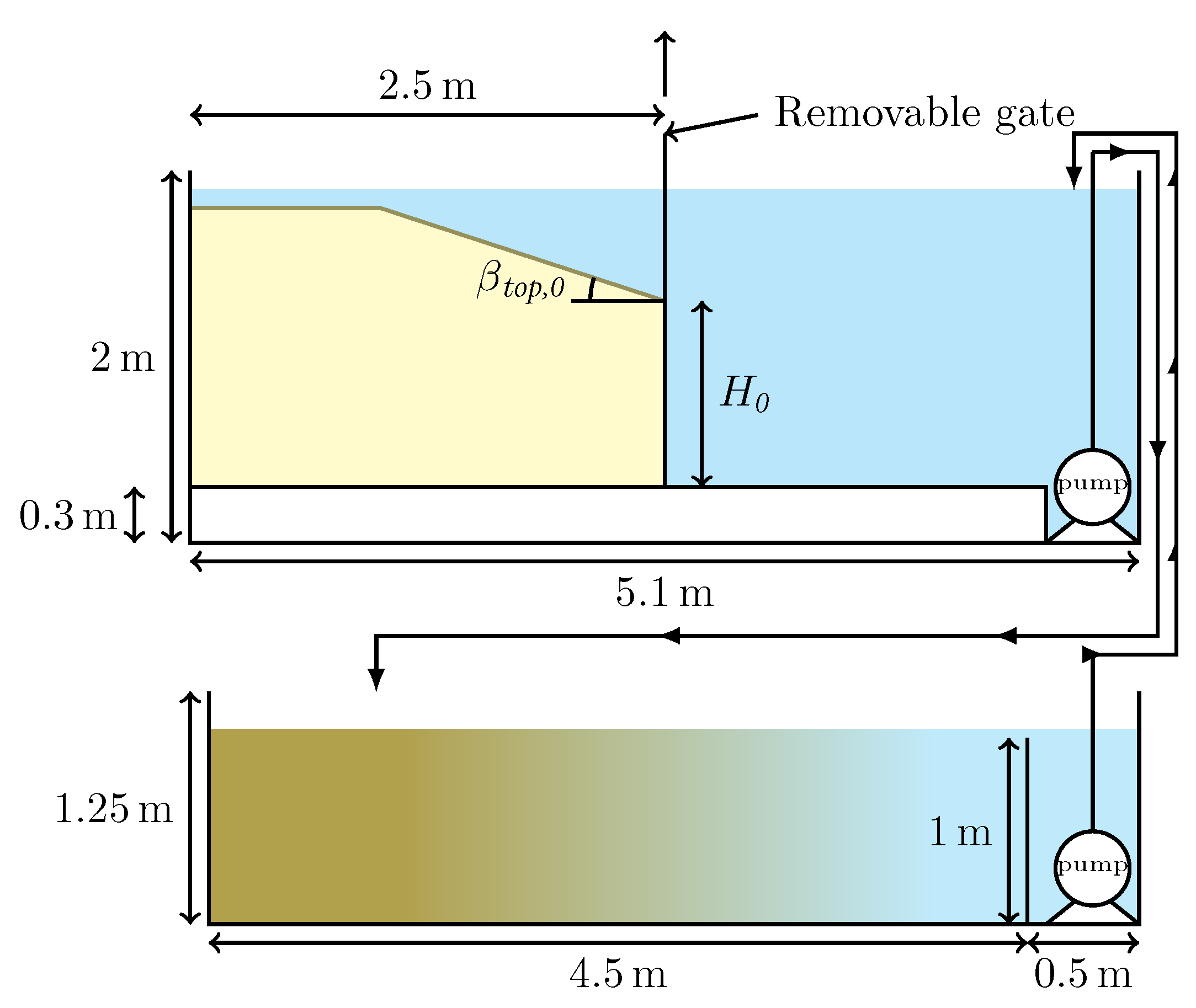
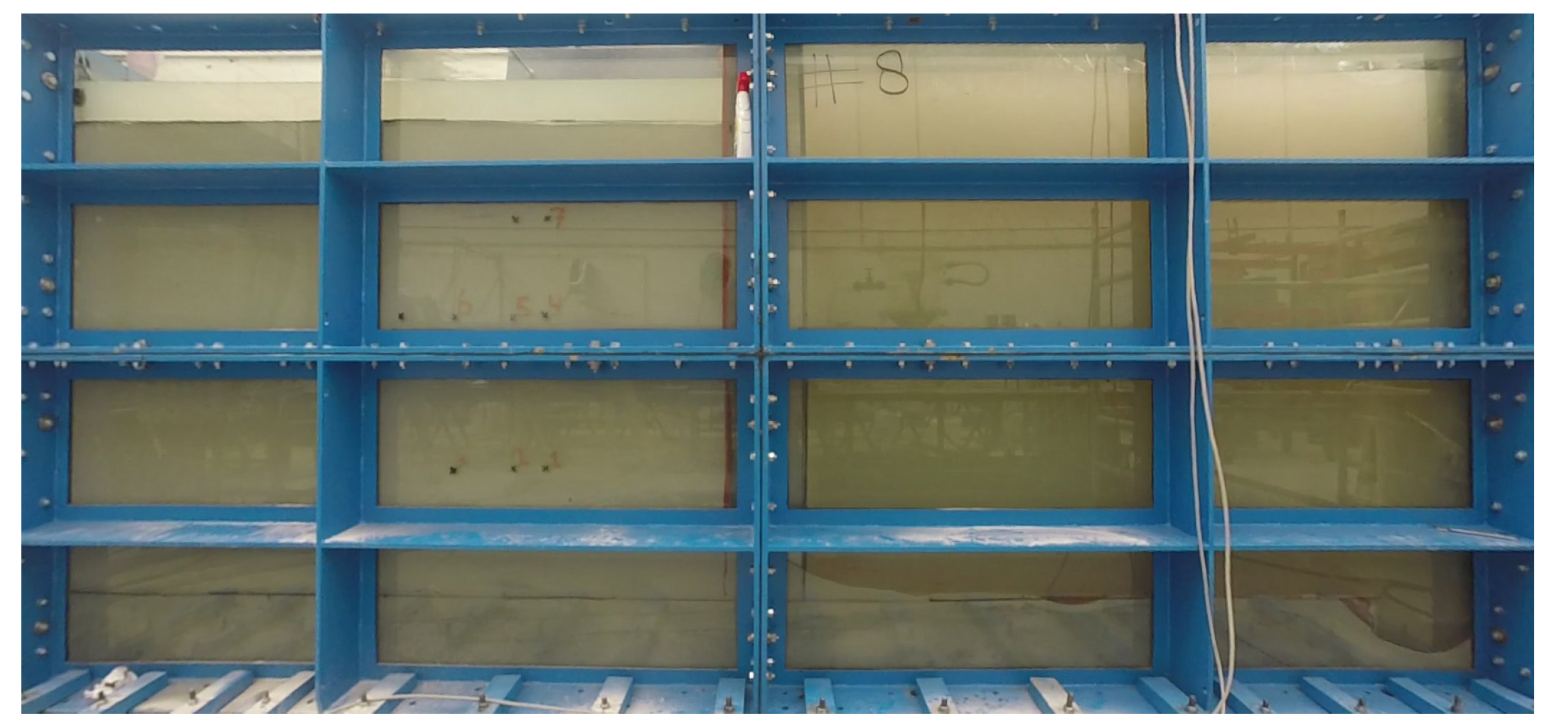
3.1. Experimental Setup

The experimental setup is composed of several components: a breaching tank, impermeable removable gate, false floor, and sedimentation tank (see Figure 5). The breaching tank is 5.1 m long, 0.5 m wide, and 2 m high. The front side of this tank is made of glass to facilitate failure tracking and flow visualization (see Figure 6). Since the current knowledge about the triggering mechanisms of breaching flow slides is very limited [1], the experiments were carried out for over-steepened vertical slopes, which initially fail due to the gravitational force. An impermeable removable gate is used to prevent the failure of sand during the construction process of the sand deposit and to shape the vertical breach face.

A false floor of a height of 0.3 m and a length of 4.8 m is placed at the bottom of the tank to create a 0.3 m high pump sump at the right end of the tank. A centrifugal pump is mounted there to prevent the reflection of the turbidity current back upstream; the sand–water mixture is pumped out from the pump sump to a sedimentation tank, which is 4.5 m long, 1.25 m wide, and 1.25 m high. On the other side of the sedimentation tank, a second submersible pump is placed behind a 1 m high dividing wall, which pumps clean water back into the breaching tank, so as to maintain a constant water level therein.

3.2. Characterization of Sands

In the experiments, two types of sand are used, namely GEBA and D9, the properties of which are summarized in Table 1. The initial porosity, $n_0$, of each sand type was determined by taking samples before the start of the experiments for two experiments with GEBA sand, and two experiments with D9 sand. The median and 15th percentile grain size, $D_{50}$ and $D_{15}$, were determined using sieve analysis tests. The internal friction angle, $\varphi$, was determined using direct shear tests.

Table 1. Properties of the sands used in the experiments.

	${\mathit{D}}_{50}$ ($\mathsf{\mu }$m)	${\mathit{D}}_{15}$ ($\mathsf{\mu }$m)	${\mathit{n}}_0$ (-)	$\mathit{\varphi }$ (${}^{°}$)
GEBA	120	80	0.415	35.8
D9	330	225	0.430	40.1

Table 1. Properties of the sands used in the experiments.

	${\mathit{D}}_{50}$ ($\mathsf{\mu }$m)	${\mathit{D}}_{15}$ ($\mathsf{\mu }$m)	${\mathit{n}}_0$ (-)	$\mathit{\varphi }$ (${}^{°}$)
GEBA	120	80	0.415	35.8
D9	330	225	0.430	40.1

3.3. Test Procedure

Each experiment was executed following the next sequence of steps:

• The false floor is placed at the bottom of the breaching tank.
• The breaching tank is filled with clean water.
• The removable gate is lowered down until it reaches the bottom of the breaching tank.
• A layer of sand is placed into the breaching tank and compacted by a vibrator needle.
• The previous step is repeated until reaching the target breach height, $H_0$, which was up to $1.47$ m.
• For some experimental runs, a slope at the crest of the breach face is formed. The angle of this slope, ${\beta }_{top,0}$, was up to 30${}^{°}$.
• The pumps are switched on and then the gate is automatically removed, which takes about 10–17 s depending on the initial breach height.

Table 2. A summary of the experiments conducted within this study. $H_0$ is the breach height and ${\beta }_{top,0}$ is the angle of the slope at the top of the breach face, both at the start of the experiment (see Figure 5).

Test #	${\mathit{H}}_0$ (m)	${\mathit{\beta }}_{\mathit{top},0}$ (${}^{°}$)	Sand Type
1	0.66	0	GEBA
2	0.66	0	GEBA
3	0.66	0	GEBA
4	1.17	0	GEBA
5	1.17	0	GEBA
6	1.17	0	GEBA
7	0.8	20	GEBA
8	1.47	0	GEBA
9	0.8	30	GEBA
10	1.47	0	GEBA
11	0.66	30	GEBA
12	0.66	20	GEBA
13	0.66	0	D9
14	1.17	0	D9
15	0.8	30	D9
16	1.47	0	D9

summarises the initial conditions of the experiments conducted within this study.

3.4. Data Analysis

After the execution of experiments, deposit profiles demonstrating the temporal evolution of the sand failure are extracted from videos recorded by a GoPro Hero 3 camera (Figure 7). From these deposit profiles, the parameters $v_{breach}$, H, and ${\beta }_{breach}$ are retrieved. This allows for robust analysis and comparison between experiments.

The breach face is defined as the portion of the slope profile where the angle is steeper than the internal friction angle. The height of the breach face, H, is the vertical distance between the start and end points of the breach face. The breach face angle, ${\beta }_{breach}$, is defined as the angle of the straight line between the start and end points of the breach wall (see Figure 8). Since the sand erosion velocity along the breach face is not uniform (due to the self-acceleration of the turbidity currents), the average velocity is considered the erosion velocity of the breach face, $v_{breach}$.

To check the reproducibility of our experiments, we have repeated some experimental runs one time or two times. For example, Experiments 1–3 have the same initial conditions (GEBA sand, $H_0$ = $0.66$ $\mathrm{m}$, ${\beta }_{top,0}$ = 0${}^{°}$), and so have Experiments 8 and 10 (GEBA sand, $H_0$ = $1.47$ $\mathrm{m}$, ${\beta }_{top,0}$ = 0${}^{°}$). The largest variations between similar experiments are $v_{breach}$ and the size of the surficial slides occurring from time to time. This is attributed to the difficulty of constructing sand deposits of the same in situ porosity, which plays a major role in the failure progression [8]. On the other hand, the total distance travelled by the breach face for experiments having identical initial conditions is found to be very similar. The differences between breach heights, breach face angles are also found to be relatively small (see, e.g., Figure 9), while analysing the data, the variance between experiments having the same initial conditions is taken into account by considering the average values.

4. Experimental Results

4.1. General Description of the Deposit Failure

Upon the removal of the gate, the underwater sand deposit starts to fail as particles peel off almost one by one under the influence of gravity, creating a shower of sand which drags the ambient water along to generate a downward turbidity current. This current makes a turn at the breach face toe and travels as a net-depositional current over the downstream region. From time to time, an internally coherent sand wedge slides down the slope (surficial slide). The size of these slides correlates with the breach height; larger breach heights result in larger slides. It was also observed that the contribution of these surficial slides to erosion is significantly larger in the case of the courser sand (D9), compared with the finer sand (GEBA). Additionally, a lower breach face angle results in less frequent surficial slides, which is in line with the observations of Alhaddad et al. [5].

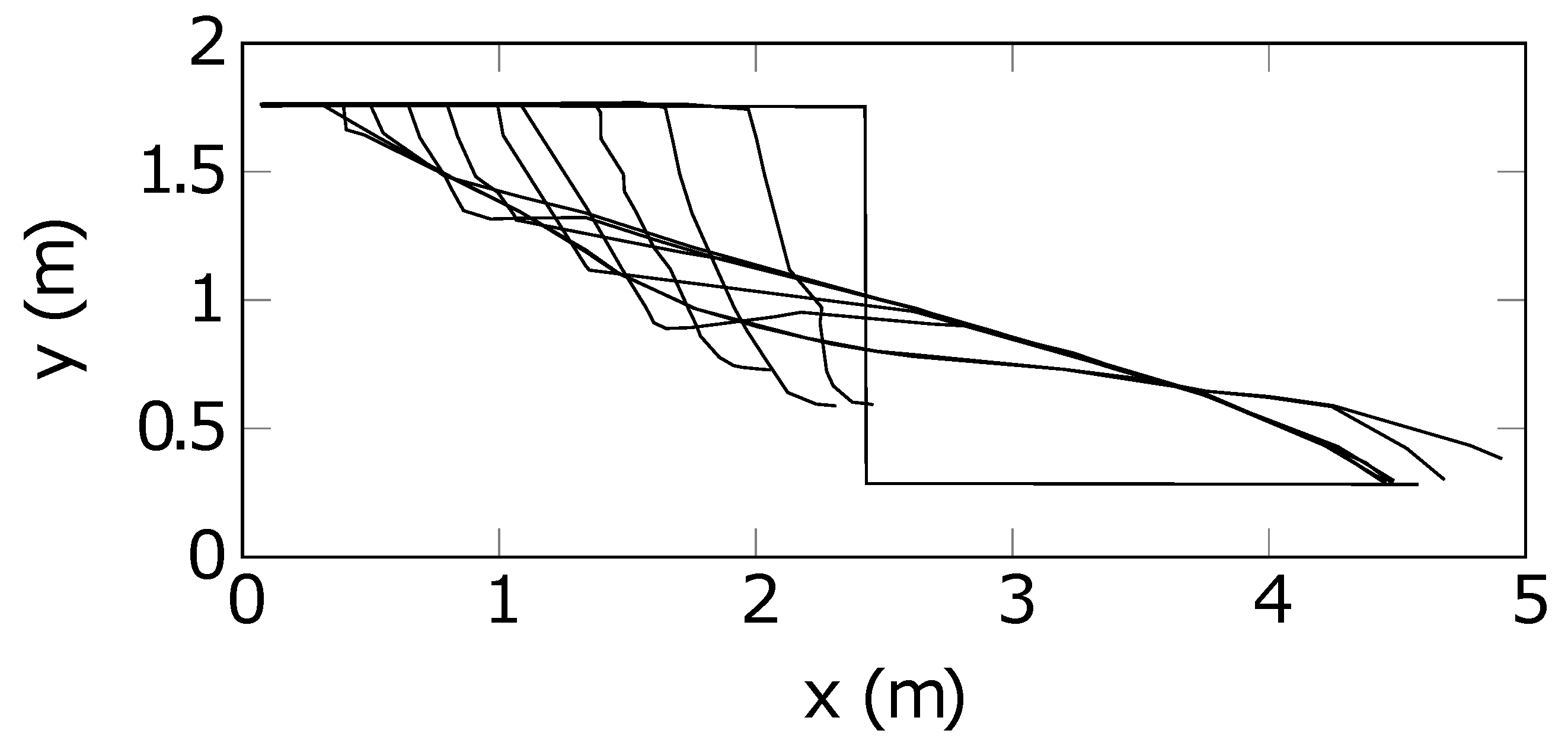
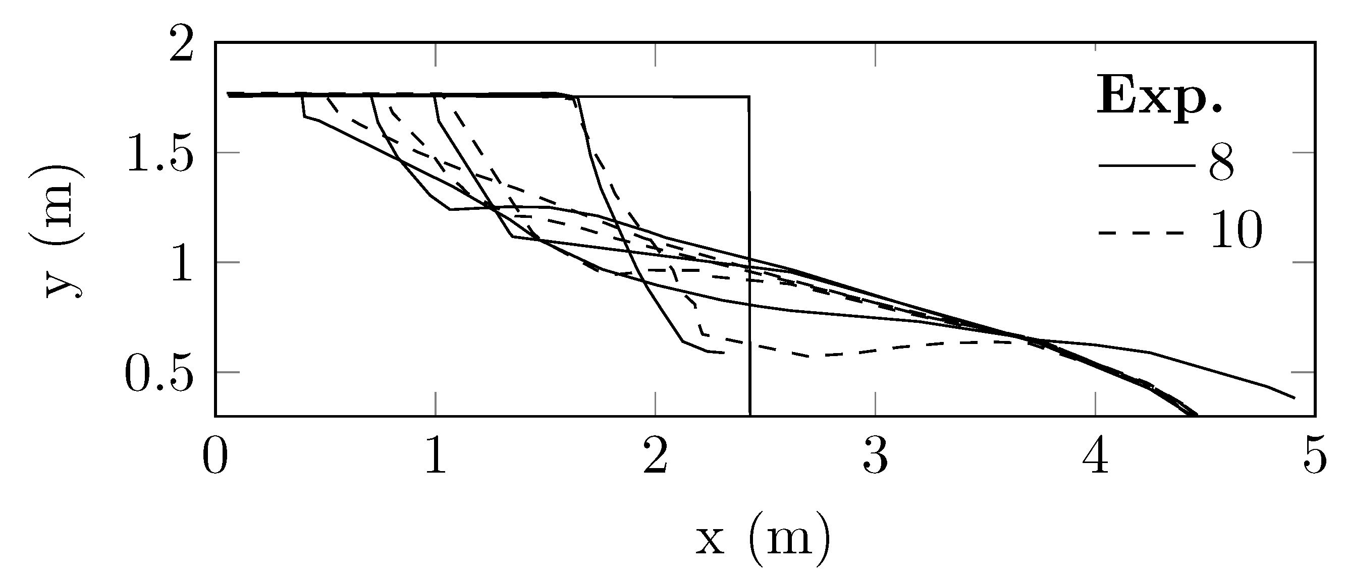
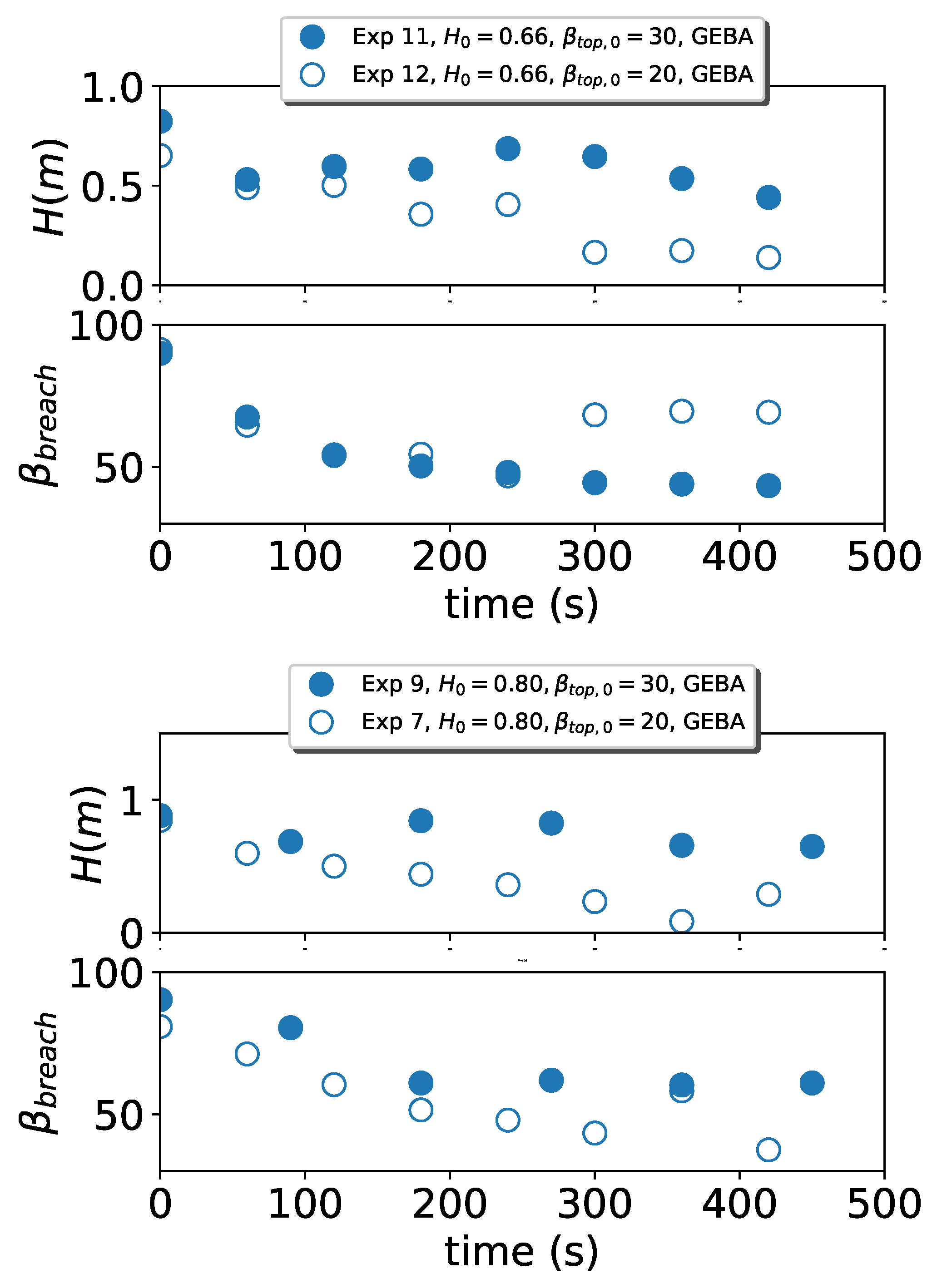
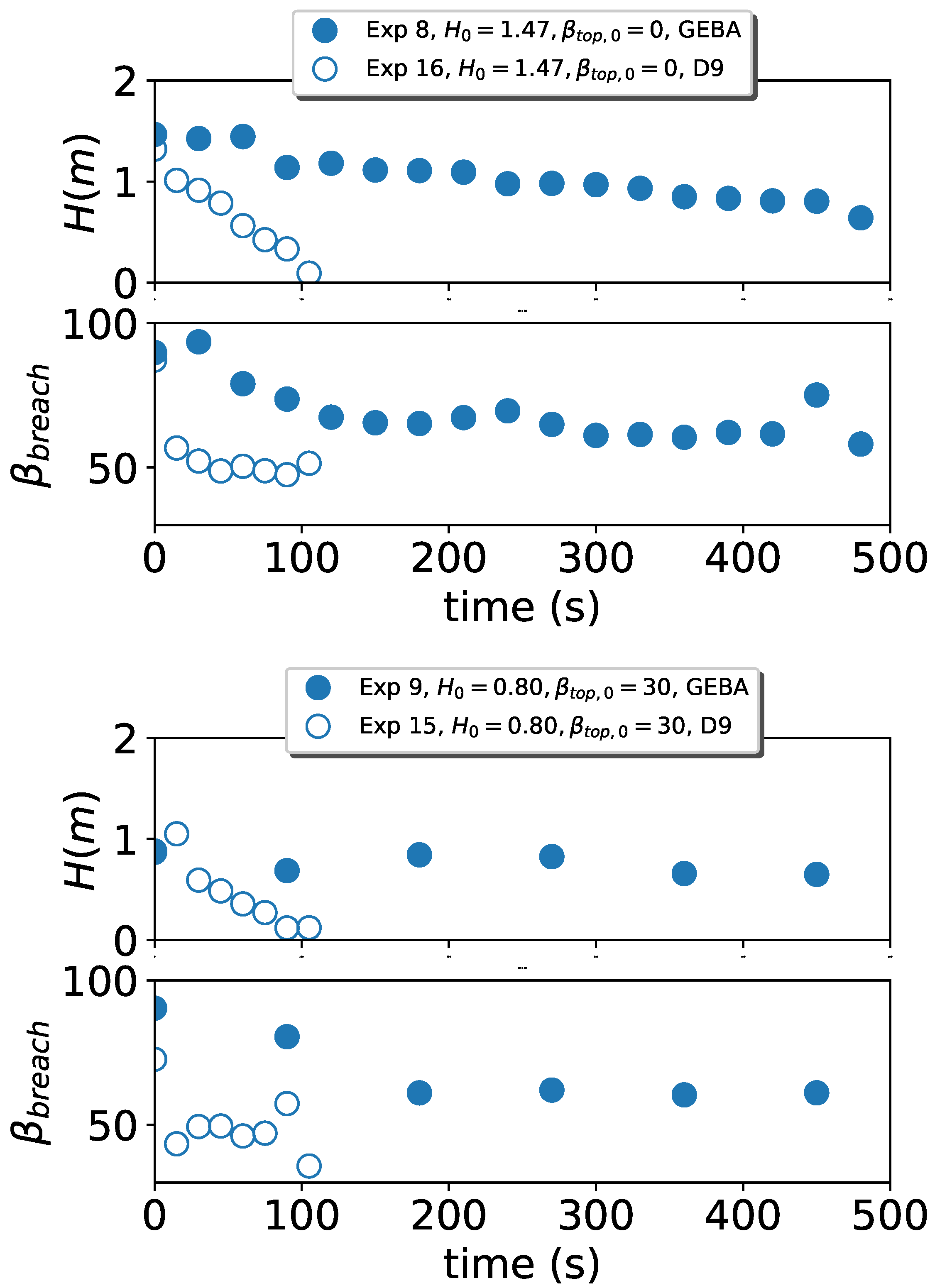
4.2. Temporal Evolution of Breaching

The temporal change of the breach height was constructed for all experimental runs. Figure 10 compares experiments with two different initial top angles, ${\beta }_{top,0}$. It is manifestly seen that the breach height remains significantly larger for the experimental runs with ${\beta }_{top,0}={30}^{°}$ compared to the experiments with an initial top angle of ${\beta }_{top,0}={20}^{°}$. This observation relates to the first term on the right-hand side of Equation (1) that describes the growth of the breach height, which is proportional to the tangent of ${\beta }_{top}$.

On the other hand, Figure 11 compares experiments with two different sand types (GEBA and D9). The breach height in the experiments with the finest sand type, GEBA, remains significantly larger compared to the experiments with the coarser sand type, D9. This observation can be attributed to both the differences in the sand hydraulic conductivities and grain sizes. The sand hydraulic conductivity largely affects the erosion velocity of the breach face, see Equation (9), which controls the time scale of the breaching process, since $dH/dt=v_{breach}dH/dx$. The grain size affects the sedimentation process at the toe of the breach face and thus the loss of breach height according to the second term on the right-hand side of Equation (1).

The breaching mode can be determined by looking at the temporal change of the breach height. For instance, results of Experiments 8 and 16 show that both breaching failures were invariably stabilizing throughout the experiments (see Figure 11 top). In addition, transition from stabilizing to destabilizing breaching is observed during Experiment 11 at time ≃ 60 s, and vice versa at time ≃ 230 s (see Figure 10 top).

5. Validity Investigation of Existing Assessment Method

In this section, we examine the validity of the assessment method presented in Section 2 based on our experimental measurements. Following that, we raise discussion points and define research directions to allow for a robust assessment of the failure mode of breaching.

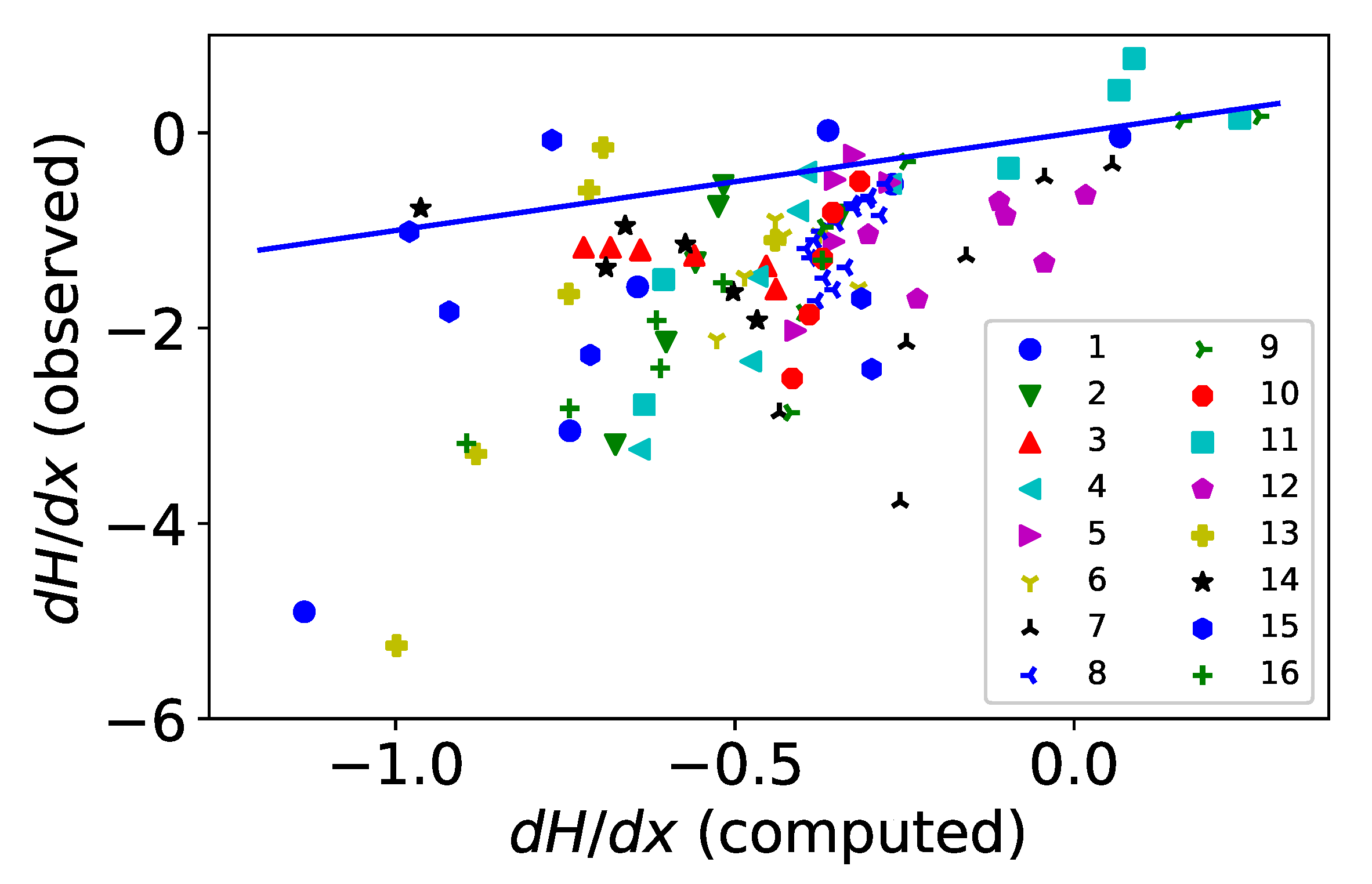
5.1. Comparison of Results

As a result of the finite size of our experimental setup, the number of observations with a clear destabilizing mode $dH/dx>0$ and thus $dH/dt>0$ is very limited. Alternatively, we here investigate the validity of the equation for $H_{crit}$ (Equation (8)) by examining the underlying relations for $dH/dx$.

Figure 12 demonstrates that the combination of Equations (1) and (3)–(5), which yields the criterion of Equation (8), is not supported by the present experimental data. This can be further quantified by using the mean absolute percentage error (MAPE) defined as,

$$\mathrm{MAPE}=\frac{100}{N}\sum _1^N\left|\frac{{(dH/dx)}_o-{(dH/dx)}_c}{{(dH/dx)}_o}\right|,$$

(10)

where ${(dH/dx)}_o$ denotes experimental observations of $dH/dx$, ${(dH/dx)}_c$ denotes the corresponding computed values, and the summation runs over all N observations shown in Figure 12. The MAPE is 92%, which demonstrates a substantial deviation. The observed $dH/dx$ is significantly smaller than the computed $dH/dx$ in most cases. This large discrepancy could be attributed to several factors. Firstly, the deviation of the geometrical simplification of the breaching process shown in Figure 2. A large number of the momentary profiles presented in Figure 7 and Figure 9 typically show the development of a plateau at the toe of breach face, after which a slope is developed. The presence of the observed plateau is not taken into account in the assessment method. Secondly, the sedimentation process at the region down the toe is complex. The turbidity current that develops at the breach face impinges at the toe and subsequently continues along the toe slope. The formation of the bed in these conditions can substantially differ from the sand fill study of Mastbergen et al. [14]. This raises questions about the applicability of Equation (3) for breaching. Thirdly, the time variation of the breach face height and toe angle, as shown in Figure 10 and Figure 11, is not taken into account in the derivation of Equation (8). In other words, the steady slope angle in the experiments of Mastbergen et al. [14] was observed after some time within which the sand flux was constant. This time is not available during breaching due to the dynamic nature of the breach face; the breach height varies over time and the breach face moves continuously backward as a result of sediment erosion. Lastly, the effect of surficial slides is not considered in the assessment method.

5.2. Outlook

In the previous subsection, we revealed that the existing assessment method of the breaching mode is unreliable. The process is geometrically more complicated than suggested by Equation (1). In fact, the sedimentation process at the toe is not in equilibrium with the instantaneous sand flux, resulting in Equation (3) being unsuitable here. It is not straightforward to correct these issues in an analytical way. Therefore, to advance our predictive capability of the breaching mode, all physical processes discussed in the previous subsection should be taken into account in a robust numerical model. This implies that numerical simulations must be capable of reproducing the hydrodynamics and sediment transport of breaching-generated turbidity currents [5]. This is because the influence of the turbidity current largely determines whether the breaching process is stabilizing or destabilizing [6]. When the turbidity current deposits sediment at the breach face toe, the breach height will gradually decrease and eventually disappear. In contrast, if the turbidity current erodes sediment at the breach face toe, the breach height will increase over time, resulting in destabilizing breaching.

Moreover, the simulation of the turbidity current should be coupled to an advanced soil model that incorporates the dilation of sand and associated pore pressure feedback. Recently it was found that soil dilatancy and pore pressure feedback can be incorporated in a fluid mechanical model of tilted sand layers with a variable in situ relative density [17,18]. This gives an interesting perspective to model the complete soil and hydromechanical interaction underlying the breaching process in the foreseeable future. Given the three dimensionality of the breaching problem [5], 3D numerical simulations would also be necessary for accurate prediction of the breaching mode.

6. Conclusions

The ability to assess whether the failure during breaching will gradually grow in size (destabilizing breaching) or diminish (stabilizing breaching) is critical for the safety of nearby and remote underwater infrastructure as well as flood defence structures. To this end, an empirical assessment method has been developed and applied in previous studies of breaching. In this study, we evaluated the performance of this method using our unique data of large-scale experiments, where we observed both failure modes. A large discrepancy is found between the experimental data and the outcome of the underlying formula of the existing assessment method. The mean absolute percentage error was found to be 92%. Although the method is useful to acquire some qualitative understanding of the progression of breaching, it is unreliable for quantitative assessment. A more fundamental 3D approach is essential to capture breach face dynamics, breaching-generated turbidity currents, occurrence of surficial slides, and sedimentation processes at the toe of the breach face.

References

1. Alhaddad, S.; Labeur, R.J.; Uijttewaal, W. Breaching Flow Slides and the Associated Turbidity Current. J. Mar. Sci. Eng. 2020, 8, 67. [Google Scholar] [CrossRef] [Green Version]
2. Alhaddad, S.; Labeur, R.J.; Uijttewaal, W. The need for experimental studies on breaching flow slides. In Proceedings of the Second International Conference on the Material Point Method for Modelling Soil-Water-Structure Interaction, Cambridge, UK, 8–10 January 2019; pp. 166–172. [Google Scholar]
3. Van Rhee, C.; Bezuijen, A. The breaching of sand investigated in large-scale model tests. In Proceedings of the 26th International Conference on Coastal Engineering, Copenhagen, Denmark, 22–26 June 1998; pp. 2509–2519. [Google Scholar]
4. Mastbergen, D.R.; Van Den Berg, J.H. Breaching in fine sands and the generation of sustained turbidity currents in submarine canyons. Sedimentology 2003, 50, 625–637. [Google Scholar] [CrossRef]
5. Alhaddad, S.; Labeur, R.J.; Uijttewaal, W. Large-scale Experiments on Breaching Flow Slides and the Associated Turbidity Current. J. Geophys. Res. Earth Surf. 2020, 125, e2020JF005582. [Google Scholar] [CrossRef]
6. Van Rhee, C. Slope failure by unstable breaching. In Proceedings of the Institution of Civil Engineers-Maritime Engineering; Thomas Telford Ltd.: London, UK, 2015; Volume 168, pp. 84–92. [Google Scholar]
7. Weij, D.; Keetels, G.; Goeree, J.; Van Rhee, C. An approach to research of the breaching process. In Proceedings of the WODCON XXI, Miami, FL, USA, 13–17 June 2016; pp. 13–17. [Google Scholar]
8. Alhaddad, S.; de Wit, L.; Labeur, R.J.; Uijttewaal, W. Modeling of Breaching-Generated Turbidity Currents Using Large Eddy Simulation. J. Mar. Sci. Eng. 2020, 8, 728. [Google Scholar] [CrossRef]
9. Eke, E.; Viparelli, E.; Parker, G. Field-scale numerical modeling of breaching as a mechanism for generating continuous turbidity currents. Geosphere 2011, 7, 1063–1076. [Google Scholar] [CrossRef]
10. You, Y.; Flemings, P.; Mohrig, D. Mechanics of dual-mode dilative failure in subaqueous sediment deposits. Earth Planet. Sci. Lett. 2014, 397, 10–18. [Google Scholar] [CrossRef]
11. Mastbergen, D.R.; Beinssen, K.; Nédélec, Y. Watching the Beach Steadily Disappearing: The Evolution of Understanding of Retrogressive Breach Failures. J. Mar. Sci. Eng. 2019, 7, 368. [Google Scholar] [CrossRef] [Green Version]
12. Alhaddad, S.; Labeur, R.; Uijttewaal, W. Preliminary Evaluation of Existing Breaching Erosion Models. In Proceedings of the 10th International Conference on Scour and Erosion, ISSMGE, Arlington, VA, USA, 18–20 October 2021; pp. 619–627. [Google Scholar]
13. Van Rhee, C. Simulation of the breaching process—Experimental validation. In Proceedings of the 22nd World Dredging Conference, Changhai, China, 25–29 April 2019. [Google Scholar]
14. Mastbergen, D.; Winterwerp, J.; Bezuijen, A. On the construction of sand fill dams. Part 1: Hydraulic aspects. In Modelling Soil-Water Structure Interaction; Kolkman, P.A., Lindenberg, J., Pilarczyk, K.W., Eds.; CRC Press: Delft, The Netherlands, 1988; pp. 353–362. [Google Scholar]
15. Eke, E.; Parker, G.; Wang, R. Breaching as a mechanism for generating sustained turbidity currents. In Proceedings of the 33rd Internation Association of Hydraulic Engineering & Research Congress: Water Engineering for a Sustainable Environment; IAHR: Vancouver, BC, Canada, 2009. [Google Scholar]
16. You, Y.; Flemings, P.; Mohrig, D. Dynamics of dilative slope failure. Geology 2012, 40, 663–666. [Google Scholar] [CrossRef] [Green Version]
17. Montellà, E.; Chauchat, J.; Chareyre, B.; Bonamy, C.; Hsu, T. A two-fluid model for immersed granular avalanches with dilatancy effects. J. Fluid Mech. 2021, 925. [Google Scholar] [CrossRef]
18. Lee, C.H.; Chen, J.Y. Multiphase simulations and experiments of subaqueous granular collapse on an inclined plane in densely packed conditions: Effects of particle size and initial concentration. Phys. Rev. Fluids 2022, 7, 044301. [Google Scholar] [CrossRef]
Figure 1. Diagrammatic illustration of the breaching modes, stabilizing breaching (left), and destabilizing breaching (right); H is the breach height.
Jmse 11 00560 g001
Figure 2. Schematic overview of a 2D breaching failure. During a time interval Δ t the breach face moves over a distance Δ x and the slope at the toe progresses by sedimentation over the same distance. It is assumed that during this interval the angles β t o p and β t o e remain constant.
Jmse 11 00560 g002
Figure 3. Steady slope angle, β f i l l , produced in an experimental run by Mastbergen et al. [14].
Jmse 11 00560 g003
Figure 4. Illustration of the criterion expressed by Equation (8). For a given sand type and in situ porosity, the breaching mode is determined by three parameters: the breach height H, the angle of the breach face β b r e a c h and the the slope angle at the top of the breach face β t o p . The criterion curve is plotted for three angles of the breach face: 90 ° , 70 ° , and 50 ° . For a given breach face angle, the corresponding contour line separates the regions in the ( H , β t o p ) plane that result in d H / d x < 0 (left side of dashed line, stabilizing) and d H / d x > 0 (right side of dashed line, destabilizing). Sand parameters correspond with GEBA type as defined in Table 1 and n 1 = 0.455 .
Jmse 11 00560 g004
Figure 5. Front view of the experimental setup illustrating all components: breaching tank (Top) and sedimentation tank (Bottom).
Jmse 11 00560 g005
Figure 6. Front side of the breaching tank just before Experiment 8. The view is partially obstructed by the vertical steel bars in the middle of the tank.
Jmse 11 00560 g006
Figure 7. Deposit profiles plotted every 90 s for Experiment 8. Linear interpolation was used for obscured parts by the vertical steel bars.
Jmse 11 00560 g007
Figure 8. Definitions used for the breach height, H, and breach face angle, β b r e a c h .
Jmse 11 00560 g008
Figure 9. Profiles plotted at 0, 180, 410, 600, and 810 s for Experiments 8 and 10.
Jmse 11 00560 g009
Figure 10. Effect of the initial angle of the slope at the top of the breach face, β t o p , 0 , on the temporal evolution of the breach height, H, and breach face angle, β b r e a c h .
Jmse 11 00560 g010
Figure 11. Effect of sand type on the temporal evolution of the breach height, H, and breach face angle, β b r e a c h .
Jmse 11 00560 g011
Figure 12. Observed change of the breach height d H / d x in Experiments 1-16 versus the computed d H / d x using Equations (1) and (3)–(5). The solid line represents perfect agreement.
Jmse 11 00560 g012