
Development and Control of an Innovative Underwater Vehicle Manipulator System


Abstract
:1. Introduction
- A novel concept of a dual-arm UVMS with manipulators as its core is proposed, the mechanical structure is designed in detail based on the modular design approach, and the control architecture is constructed based on the Robot Operating System (ROS).
- The dynamic model of FAUVMS that considers dynamic coupling is developed, and the RNEM is used to evaluate the dynamic coupling effects in the system.
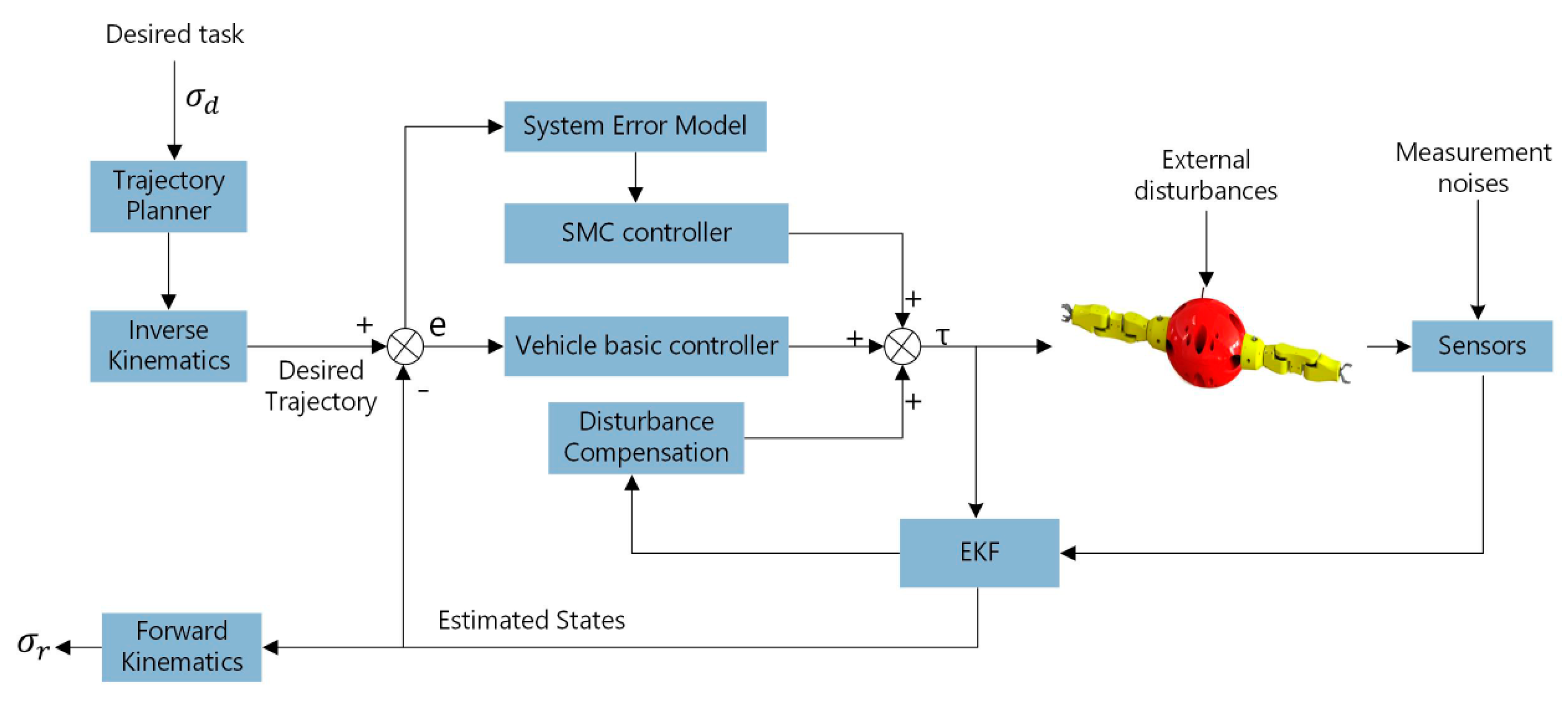
- A robust adaptive controller is designed based on CTC, EKF and chattering-free SMC, and the closed-loop stability is guaranteed by Lyapunov theory.
- The simulation platform for FAUVMS is proposed based on Gazebo and the unmanned underwater vehicle simulator (UUVSimulator), and simulations are carried out to verify the effectiveness of the proposed control method.
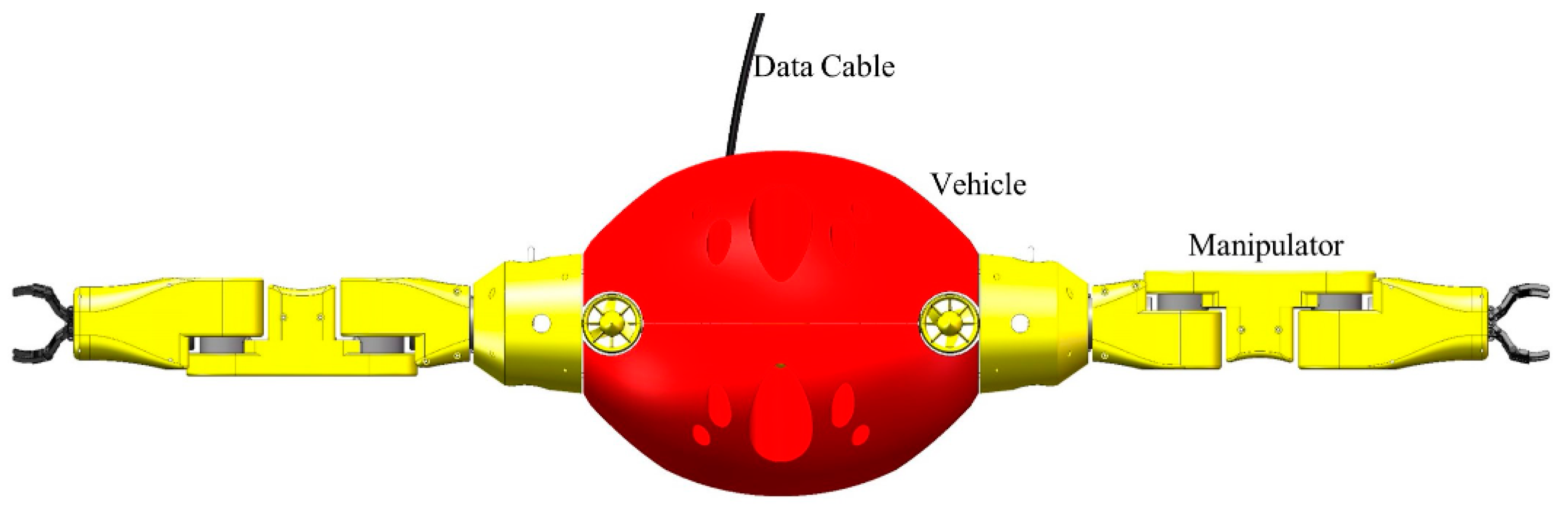
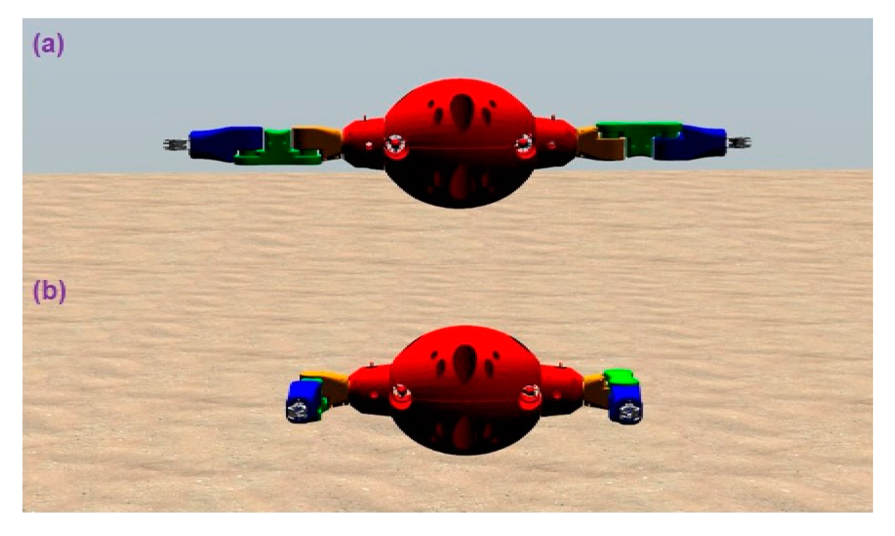
2. Design of FAUVMS
2.1. Mechanical Structure
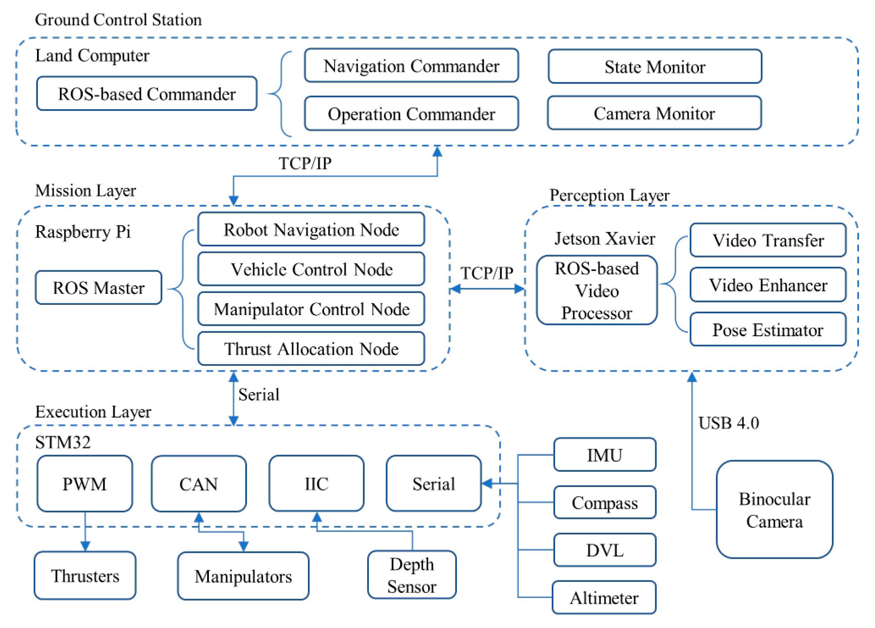
2.2. Control Architecture
2.2.1. Ground Control Station
2.2.2. Mission Layer
2.2.3. Execution Layer
2.2.4. Perception Layer
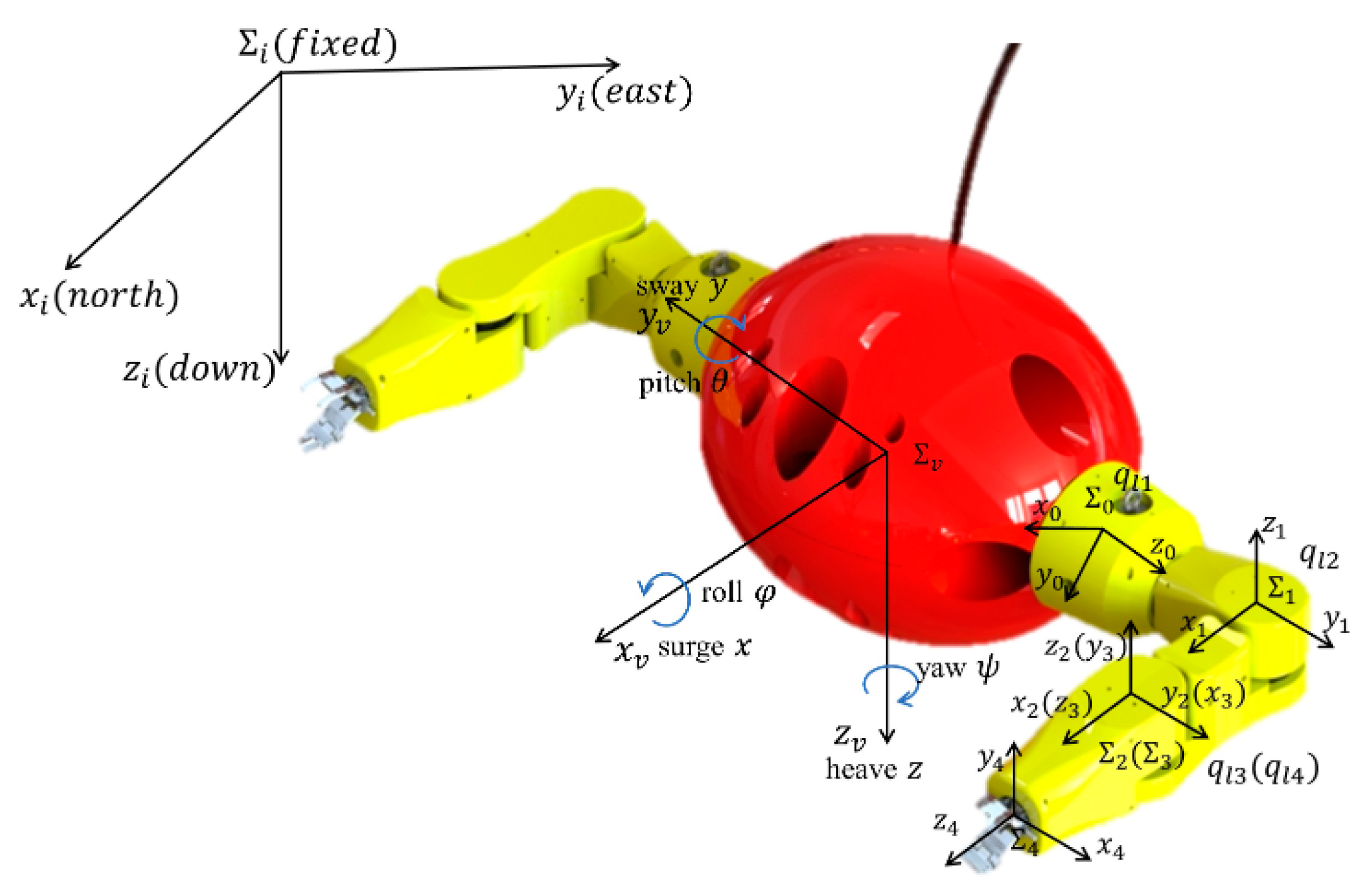
3. Dynamic Modeling of FAUVMS
3.1. General Model of FAUVMS
3.2. Coupling Force Estimation
4. Robust Adaptive Control of FAUVMS
4.1. EKF Disturbance Observer Design
4.2. Chattering-Free Sliding Mode Controller Design
- (i)
- In the absence of uncompensated disturbances, i.e., , the system error will converge to zero in finite time.
- (ii)
- In the presence of uncompensated disturbances, i.e., , the system error will converge to the regionin finite time, where and are the minimum eigenvalues of and . In addition, the position errors and velocity errors converge to the regions
5. Simulation and Analysis
5.1. Description of the Simulation Platform
5.2. Description of the Scenarios
5.3. Results and Discussion
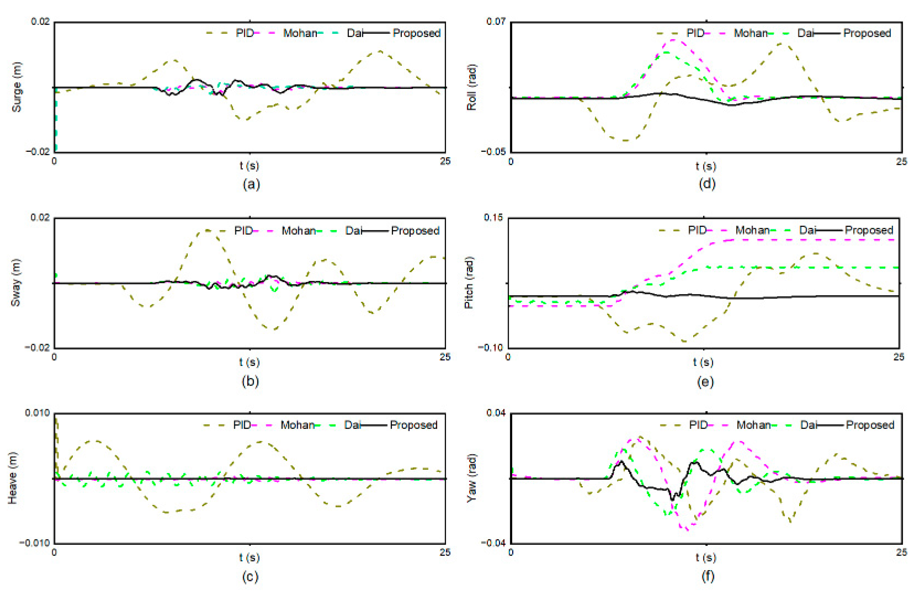
5.3.1. Scenario 1
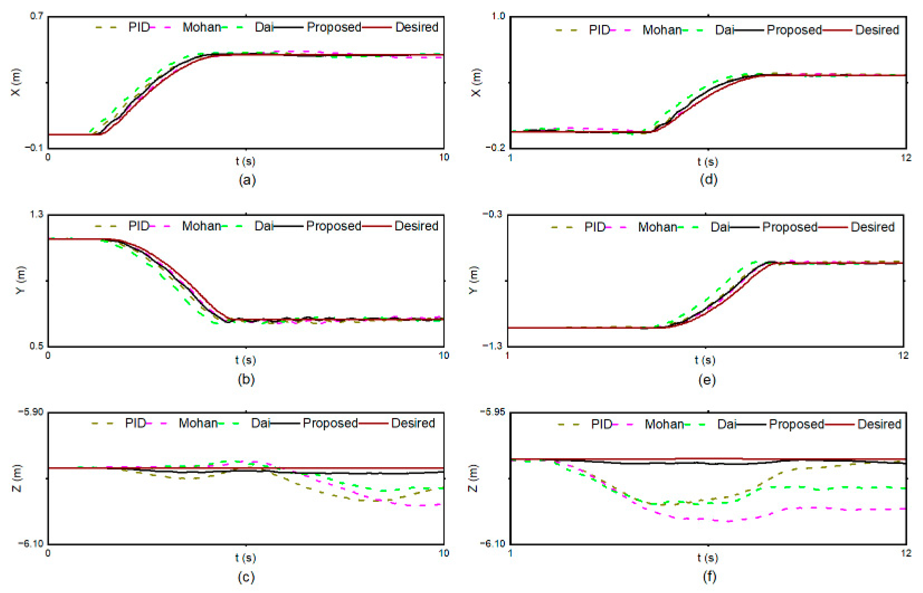
5.3.2. Scenario 2
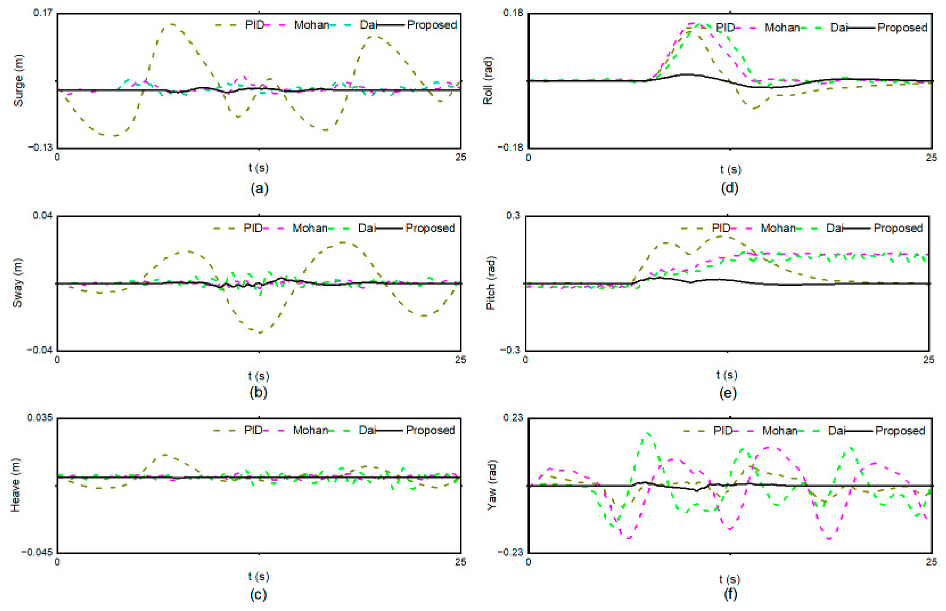
5.3.3. Scenario 3
6. Conclusions
Supplementary Materials
Author Contributions
Funding
Institutional Review Board Statement
Informed Consent Statement
Data Availability Statement
Acknowledgments
Conflicts of Interest
References
- Wang, Y.; Bai, X.; Cheng, L.; Wang, S.; Tan, M. Data-Driven Hydrodynamic Modeling for a Flippers-Driven Underwater Vehicle-Manipulator System. In Proceedings of the 9th IEEE Data Driven Control and Learning Systems Conference (DDCLS), Liuzhou, China, 19–21 June 2020; pp. 342–349. [Google Scholar]
- Hachicha, S.; Zaoui, C.; Dallagi, H.; Nejim, S.; Maalej, A. Innovative design of an underwater cleaning robot with a two arm manipulator for hull cleaning. Ocean Eng. 2019, 181, 303–313. [Google Scholar] [CrossRef]
- Jones, D.O.B. Using existing industrial remotely operated vehicles for deep-sea science. Zool. Scr. 2009, 38, 41–47. [Google Scholar] [CrossRef]
- Chang, C.C.; Chang, C.Y.; Cheng, Y.T. Distance measurement technology development at remotely teleoperated robotic manipulator system for underwater constructions. In Proceedings of the 2004 International Symposium on Underwater Technology, Howard International House, Taipei, Taiwan, 20–23 April 2004; pp. 333–338. [Google Scholar] [CrossRef]
- Cui, W. Development of the Jiaolong deep manned submersible. Mar. Technol. Soc. J. 2013, 47, 37–54. [Google Scholar] [CrossRef]
- Ribas, D.; Palomeras, N.; Ridao, P.; Carreras, M.; Mallios, A. Girona 500 AUV: From Survey to Intervention. IEEE/ASME Trans. Mechatron. 2012, 17, 46–53. [Google Scholar] [CrossRef]
- Wang, Y.; Cai, M.; Wang, S.; Bai, X.; Wang, R.; Tan, M. Development and Control of an Underwater Vehicle-Manipulator System Propelled by Flexible Flippers for Grasping Marine Organisms. IEEE Trans. Ind. Electron. 2022, 69, 3898–3908. [Google Scholar] [CrossRef]
- Bae, J.; Bak, J.; Jin, S.; Seo, T.; Kim, J. Optimal configuration and parametric design of an underwater vehicle manipulator system for a valve task. Mech. Mach. Theory 2018, 123, 76–88. [Google Scholar] [CrossRef]
- Bae, J.; Moon, Y.; Park, E.; Kim, J.; Jin, S.; Seo, T. Cooperative Underwater Vehicle-Manipulator Operation Using Redundant Resolution Method. Int. J. Precis. Eng. Manuf. 2022, 23, 1003–1017. [Google Scholar] [CrossRef]
- Bae, J.; Jin, S.; Kim, J.; Seo, T. Comparative study on underwater manipulation methods for valve-turning operation. Meccanica 2019, 54, 901–916. [Google Scholar] [CrossRef]
- Leabourne, K.N. Two-Link Hydrodynamic Model Development and Motion Planning for Underwater Manipulation. Ph.D. Thesis, Stanford University, Stanford, CA, USA, 2001. [Google Scholar]
- Sivcev, S.; Coleman, J.; Omerdic, E.; Dooly, G.; Toal, D. Underwater manipulators: A review. Ocean Eng. 2018, 163, 431–450. [Google Scholar] [CrossRef]
- Han, J.; Chung, W.K. Active Use of Restoring Moments for Motion Control of an Underwater Vehicle-Manipulator System. IEEE J. Ocean. Eng. 2014, 39, 100–109. [Google Scholar] [CrossRef]
- Esfahani, H.N.; Azimirad, V.; Danesh, M. A Time Delay Controller included terminal sliding mode and fuzzy gain tuning for Underwater Vehicle-Manipulator Systems. Ocean Eng. 2015, 107, 97–107. [Google Scholar] [CrossRef]
- Chen, W.; Wei, M.; Zhang, Y.; Lu, D.; Hu, S. Research on Adaptive Sliding Mode Control of UVMS Based on Nonlinear Disturbance Observation. Math. Probl. Eng. 2022, 2022, 6908399. [Google Scholar] [CrossRef]
- Dong, X.; Ren, C.; He, S.; Cheng, L.; Wang, S. FINITE-TIME SLIDING MODE CONTROL FOR UVMS VIA T-S FUZZY APPROACH. Discret. Contin. Dyn. Syst. 2021, 15, 1699–1712. [Google Scholar] [CrossRef]
- Yu, X.; Zhihong, M. Multi-input uncertain linear systems with terminal sliding-mode control**This paper was recommended for publication in revised form by Editor Professor P. Dorato. Automatica 1998, 34, 389–392. [Google Scholar] [CrossRef]
- Yu, S.; Yu, X.; Shirinzadeh, B.; Man, Z. Continuous finite-time control for robotic manipulators with terminal sliding mode. Automatica 2005, 41, 1957–1964. [Google Scholar] [CrossRef]
- Du, H.; Yu, X.; Chen, M.Z.Q.; Li, S. Chattering-free discrete-time sliding mode control. Automatica 2016, 68, 87–91. [Google Scholar] [CrossRef]
- Dai, Y.; Yu, S.; Yan, Y.; Yu, X. An EKF-Based Fast Tube MPC Scheme for Moving Target Tracking of a Redundant Underwater Vehicle-Manipulator System. IEEE/ASME Trans. Mechatron. 2019, 24, 2803–2814. [Google Scholar] [CrossRef]
- Dehkordi, S.F. Dynamic analysis of flexible-link manipulator in underwater applications using Gibbs-Appell formulations. Ocean Eng. 2021, 241, 110057. [Google Scholar] [CrossRef]
- Xiong, X.; Xiang, X.; Wang, Z.; Yang, S. On dynamic coupling effects of underwater vehicle-dual-manipulator system. Ocean Eng. 2022, 258, 111699. [Google Scholar] [CrossRef]
- Tarn, T.J.; Shoults, G.; Yang, S. A dynamic model of an underwater vehicle with a robotic manipulator using Kane’s method. Auton. Robot. 1996, 3, 269–283. [Google Scholar] [CrossRef]
- Korayem, M.H.; Hedayat, A.; Dehkordi, S.F. Dynamic modeling of cooperative manipulators with frictional contact at the end effectors. Appl. Math. Model. 2021, 90, 302–326. [Google Scholar] [CrossRef]
- Santhakumar, M. Investigation into the Dynamics and Control of an Underwater Vehicle-Manipulator System. Model. Simul. Eng. 2013, 2013, 839046. [Google Scholar] [CrossRef] [Green Version]
- Barbălată, C.; Dunnigan, M.W.; Pétillot, Y. Dynamic coupling and control issues for a lightweight underwater vehicle manipulator system. In Proceedings of the 2014 Oceans-St. John’s, St. John’s, NL, Canada, 14–19 September 2014; pp. 1–6. [Google Scholar] [CrossRef]
- Han, H.; Wei, Y.; Ye, X.; Liu, W. Motion Planning and Coordinated Control of Underwater Vehicle-Manipulator Systems with Inertial Delay Control and Fuzzy Compensator. Appl. Sci. 2020, 10, 3944. [Google Scholar] [CrossRef]
- Long, C.; Qin, X.; Bian, Y.; Hu, M. Trajectory tracking control of ROVs considering external disturbances and measurement noises using ESKF-based MPC. Ocean Eng. 2021, 241, 109991. [Google Scholar] [CrossRef]
- Mohan, S.; Kim, J. Indirect adaptive control of an autonomous underwater vehicle-manipulator system for underwater manipulation tasks. Ocean Eng. 2012, 54, 233–243. [Google Scholar] [CrossRef]
- Dai, Y.; Yu, S. Design of an indirect adaptive controller for the trajectory tracking of UVMS. Ocean Eng. 2018, 151, 234–245. [Google Scholar] [CrossRef]
- Dai, Y.; Yu, S.; Yan, Y. An adaptive EKF-FMPC for the trajectory tracking of UVMS. IEEE J. Ocean. Eng. 2019, 45, 699–713. [Google Scholar] [CrossRef]
- Görner, M.; Haschke, R.; Ritter, H.; Zhang, J. Moveit! task constructor for task-level motion planning. In Proceedings of the 2019 International Conference on Robotics and Automation (ICRA), Montreal, QC, Canada, 20–24 May 2019; IEEE: New York, NY, USA, 2019; pp. 190–196. [Google Scholar]
- Zheng, X.H.; Wang, C.; Yang, X.J.; Tian, Q.Y.; Zhang, Q.F.; Zhai, B.Q. A Novel Thrust Allocation Method for Underwater Robots. In Proceedings of the 2022 12th International Conference on CYBER Technology in Automation, Control, and Intelligent Systems (CYBER), Baishan, China, 27–31 July 2022; pp. 271–276. [Google Scholar] [CrossRef]
- Fossen, T.I. Guidance and Control of Ocean Vehicles. Doctors Thesis, University of Trondheim, Trondheim, Norway, 1999. [Google Scholar]
- Antonelli, G. Modelling of Underwater Robots. In Underwater Robots; Springer International Publishing: Cham, Switzerland, 2018; pp. 33–110. [Google Scholar] [CrossRef]
- Manhães, M.M.M.; Scherer, S.A.; Voss, M.; Douat, L.R.; Rauschenbach, T. UUV Simulator: A Gazebo-based package for underwater intervention and multi-robot simulation. In Proceedings of the OCEANS 2016 MTS/IEEE Monterey, Monterey, CA, USA, 19–23 September 2016; IEEE: New York, NY, USA, 2016. [Google Scholar] [CrossRef]


| Parameters | Values | Parameters | Values |
|---|---|---|---|
| Vehicle mass | 63 kg | Metacentric height | <5 mm |
| Vehicle length | 640 mm | Vehicle width | 450 mm |
| Vehicle height | 450 mm | Maximum depth | 1000 m |
| Max/Min thrust | 5 kg/−4 kg | Number of thrusters | 6 |
| Payload of arm | 5 kg | Number of joints | 4 |
| Link mass | 1.5/2.5/2.5/2.5 kg | Link length | 220/330/250/50 mm |
| Link radius | 60/60/60/50 mm | IMU&Compass | Pixhawk |
| Altimeter | Ping30 | Velocity logger | Waterlinked A50 |
| Parameters | Values | Parameters | Values |
|---|---|---|---|
| Inertia of vehicle | COM of vehicle | mm | |
| COB of vehicle | mm | Ellipsoid parameters A | 280 mm |
| Ellipsoid parameters B | 350 mm | Ellipsoid parameters C | 280 mm |
| Inertia of link1 | Inertia of link2 | ||
| Inertia of link3 | Inertia of link4 | ||
| COM of link1 | mm | COM of link1 | mm |
| COM of link3 | mm | COM of link4 | mm |
| Volume of Link1 | Volume of Link2 | ||
| Volume of Link3 | Volume of Link4 |
| MSE/cm | PID | Mohan | Dai | Proposed |
|---|---|---|---|---|
| Left X | 1.89 | 1.23 | 3.36 | 1.31 |
| Left Y | 2.19 | 1.39 | 3.98 | 1.65 |
| Left Z | 1.78 | 2.31 | 1.45 | 0.29 |
| Right X | 1.96 | 0.99 | 3.17 | 1.74 |
| Right Y | 2.04 | 1.24 | 3.59 | 1.69 |
| Right Z | 1.93 | 2.74 | 1.85 | 0.21 |
| MSE/cm | PID | Mohan | Dai | Proposed |
|---|---|---|---|---|
| Left X | 1.74 | 1.92 | 1.49 | 0.93 |
| Left Y | 1.95 | 2.33 | 1.35 | 1.23 |
| Left Z | 4.99 | 4.15 | 3.89 | 1.02 |
| Right X | 1.08 | 1.31 | 1.61 | 1.72 |
| Right Y | 1.59 | 2.69 | 1.13 | 1.15 |
| Right Z | 5.17 | 6.22 | 6.27 | 0.61 |
| MSE/cm | PID | Mohan | Dai | Proposed |
|---|---|---|---|---|
| Left X | 9.28 | 9.24 | 9.71 | 1.63 |
| Left Y | 1.88 | 3.37 | 4.33 | 1.59 |
| Left Z | 5.23 | 3.95 | 3.82 | 1.92 |
| Right X | 6.24 | 9.55 | 10.59 | 1.86 |
| Right Y | 0.78 | 2.05 | 2.57 | 1.34 |
| Right Z | 5.99 | 6.38 | 6.72 | 1.83 |
Disclaimer/Publisher’s Note: The statements, opinions and data contained in all publications are solely those of the individual author(s) and contributor(s) and not of MDPI and/or the editor(s). MDPI and/or the editor(s) disclaim responsibility for any injury to people or property resulting from any ideas, methods, instructions or products referred to in the content. |
© 2023 by the authors. Licensee MDPI, Basel, Switzerland. This article is an open access article distributed under the terms and conditions of the Creative Commons Attribution (CC BY) license (https://creativecommons.org/licenses/by/4.0/).
Share and Cite
Zheng, X.; Tian, Q.; Zhang, Q. Development and Control of an Innovative Underwater Vehicle Manipulator System. J. Mar. Sci. Eng. 2023, 11, 548. https://doi.org/10.3390/jmse11030548
Zheng X, Tian Q, Zhang Q. Development and Control of an Innovative Underwater Vehicle Manipulator System. Journal of Marine Science and Engineering. 2023; 11(3):548. https://doi.org/10.3390/jmse11030548
Chicago/Turabian StyleZheng, Xinhui, Qiyan Tian, and Qifeng Zhang. 2023. "Development and Control of an Innovative Underwater Vehicle Manipulator System" Journal of Marine Science and Engineering 11, no. 3: 548. https://doi.org/10.3390/jmse11030548