
Research on Bearing Characteristics of Gravity Anchor in Clay
by
 ,
,
Jianxing Yu
1,2, 
Pengfei Liu
1,2,*,
Yang Yu
1,2,
Xin Liu
1,2,
Haoda Li
1,2,
Ruoke Sun
1,2 and
Xuyang Zong
3 1
State Key Laboratory of Hydraulic Engineering Simulation and Safety, Tianjin University, Tianjin 300072, China
2
Tianjin Key Laboratory of Port and Ocean Engineering, Tianjin University, Tianjin 300072, China
3
System Engineering Research Institute, China State Shipbuilding Corporation, Beijing 100036, China
*
Author to whom correspondence should be addressed.
J. Mar. Sci. Eng. 2023, 11(3), 505; https://doi.org/10.3390/jmse11030505
Submission received: 5 February 2023
/
Revised: 16 February 2023
/
Accepted: 23 February 2023
/
Published: 26 February 2023
(This article belongs to the Special Issue Advanced Analysis of Marine Structures)
Abstract
:The applications and studies of gravity anchors in the ocean are becoming more and more extensive. Most of the research, however, has been directed toward the bearing properties of sand. Relatively less attention has been paid to the bearing properties of gravity anchors in clay. Clay is widely distributed on the seabed. The research on the bearing capacity of gravity anchors in clay is of great significance for offshore oil exploitation. Therefore, the gravity anchor was investigated by conducting reduced-scale model tests, and the bearing process of gravity anchors in clay was simulated through a 3D finite element method. Model tests and numerical simulations were used to determine the capacity curve and the V-H failure envelope of gravity anchors in clay. The simulation results and the test results are in good agreement. The failure form of the gravity anchor in clay was revealed by 3D finite element analysis. The effect of cohesion, internal friction angle, and mooring point height on bearing capacity have been studied. The influence of the height of the mooring point on the V-H failure envelope curve was explored by changing the height of the mooring point. The formula of the V-H failure envelope curve suitable for different mooring point heights was obtained.
1. Introduction
In recent years, oil and gas extraction has moved into increasingly deep water in search of energy [1]. The laying of pipelines is a key step in the process of offshore oil exploration [2]. In order to stabilize the pipe-laying ship, it is necessary to use an anchoring device for anchoring. Gravity anchors are the oldest mooring equipment. It provides horizontal and vertical bearing capacity through the reaction force of the soil [3] (it is the collection of soil forces reacting to the gravity anchor, including frictional forces, the adsorption of the soil, the soil resistance that arises when the soil is destroyed, etc.). Additionally, the gravity anchor is highly adaptable, meaning it can be used without too detailed soil survey data. Therefore, it adapts to a wide range of soil qualities and is widely used in engineering applications [4]. The surface of the seabed is mostly clay. To ensure safety in the process of offshore oil development, studying the bearing capacity characteristics of gravity anchors in clay is of great significance to the design work.
During the past decades, considerable efforts, including model tests and numerical studies, have been made to estimate the pull-out behavior of gravity anchors under loads. Harris et al. [5] outlined the general types of wave energy converters and discussed their anchoring requirements. Through experimental comparison to other anchoring systems, it was found that gravity anchor is the superior anchoring method. Comprehensive research was conducted by Yun G et al. experimentally and numerically [6]. Their study found that different buried depth ratios and different geometric shapes have a great influence on the vertical bearing capacity of gravity anchors. They proposed a calculation method for vertical bearing capacity. Taylor, R et al. [7] designed different mooring system options for the location of the Ocean Thermal Energy Conversion (OTEC). According to the environmental conditions, towed embedded anchors and gravity anchors with skirt wings were designed, and the selection of their size was discussed. Jim B. Peterson [8] invented a new type of articulated gravity anchor that is easy to operate and can provide greater bearing capacity. Three different anchor types—drilled shaft, gravity, and fluke anchors—were used to meet challenges for the new SR520 Evergreen Point Floating Bridge and Landings project in Seattle, Washington, by Upsall, B et al. [9]. Aiming at the movement mechanism of gravity anchors under compound loads, Li S [10] et al. studied the anti-sliding stability mechanism of gravity anchors through indoor model tests. The strip method was used to analyze the bearing capacity of gravity anchors under complex loads.
With the development of nonlinear methods, research on the numerical simulation of the bearing process of gravity anchors gradually increased. Houlsby G T [11] studied the numerical modeling of shallow circular foundations. Based on the numerical model results of shallow foundations on many calcareous soils combined with structural analysis, the working performance of the overall structure under dynamic loading conditions was predicted. Gourvenec S [12] studied the influence of different aspect ratios on the ultimate bearing capacity of gravity anchors by finite element analysis. Moreover, the influence of the aspect ratio on the critical state of gravity anchors under different loads is also studied in the following research. Gourvenec S [13] also examined the failure envelope of gravity anchors with skirts in uniform and inhomogeneous soils. The ultimate bearing mechanism of gravity anchors under general loads is proposed. Gourvenec S [14] studied the limit state and the kinematic mechanism of the failure of gravity anchors. The results show that the size and shape of failure envelopes defining the undrained capacity of shallow foundations under general loading are dependent on the embedment ratio. Three years later, Gourvenec S and Barnett S [15] improved the failure envelope of gravity anchors and developed the expression of the failure envelope. Bransby M F and Yun, G J [16] studied the influence of skirts on gravity anchors subjected to horizontal loads. Through model tests and finite element simulations, Niroumand H and Kassim K A [17] investigated the motion law of slab anchors under vertical loads in dense sand. The results show that the ultimate bearing capacity calculated by finite element is smaller than the ultimate bearing capacity of the model test. Based on the finite element limit analysis method, Mana, D S K et al. [18] studied the critical inner skirt plate spacing for the undrained failure of the skirt plate gravity anchor under plane strain conditions. The results showed that as the buried depth of the foundation increases, fewer inner skirts are required. Liu et al. [19] studied the pullout capacity and the keying process of a vertically installed OMNI-Max anchor embedded in normally consolidated clay by using three-dimensional large deformation finite element analysis. The analyses clearly showed two important processes: (1) “keying” in which the anchor rotates rapidly until reaching the best bearing capacity position; and (2) “diving” in which the anchor mainly translates with tiny rotation. The development of GIPLA’s movements during its keying and its pullout capacity in clay was also investigated by Liu et al. [20]. The anchor loading angle and the anchor padeye offset angle for the diving motion were suggested, and the effects of the anchor loading angle, anchor padeye eccentricity, and soil strength profile were investigated. Li, H et al. [21] studied the effect of different types of shear bonds on the bearing capacity of gravity anchors. The results showed that the horizontal bearing capacity of the eight-key anchor is greater than that of the flat-bottomed anchor. An LDFE analysis was performed to investigate the penetration and keying of GIAs by Zhao et al. [22]. Fitted formulae were also proposed to give a quick evaluation of the performance of GIAs. A numerical model on the anchor–soil–water interaction for the dynamic installation of gravity installed anchors was proposed by Liu et al. [23]. Additionally, a theoretical model was also proposed to predict the final penetration depth of the anchor. Yang et al. [24] studied a theoretical model for three-dimensional GIAs in multi-layered clays and complicated behaviors of the OMNI-Max anchor in multi-layered clays.
In this paper, the research contents of gravity anchor bearing capacity and failure envelope are expanded on the basis of the existing research. The objectives of this study are to investigate the bearing performance of gravity anchors in clay and to analyze the factors affecting the bearing performance of gravity anchors by conducting model tests and 3D finite element analysis based on the ABAQUS software package. The damage envelope curves of gravity anchors were improved based on the damage theory for shallowly buried structures.
2. Model Test
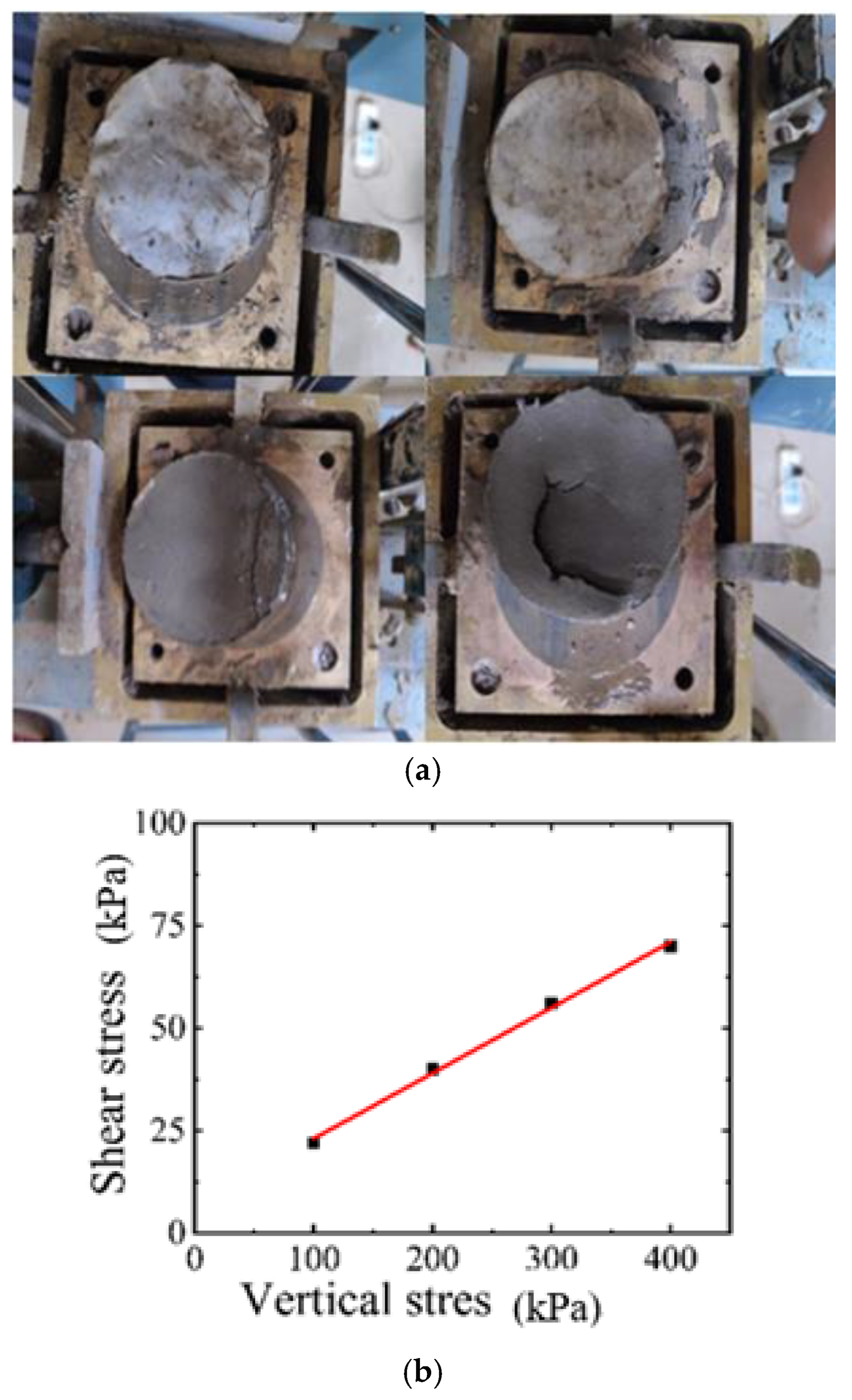
The clay used in this model test is prepared from the soil excavated from a depth of 1500 m in the South China Sea. Figure 1 is a photo taken by the author on the spot. Since there would be some impurities in the collected soil, the clay should be dried and sieved to obtain the pure clay power that can be used to prepare the test soil. The soil is fully hydrated and mixed with the aim of obtaining a homogeneous clay. Then, the soil is fully stirred, consolidated, and settled for 3 months. The purpose of consolidation settlement for 3 months is to make the soil reach the test standard. After the soil was fully saturated and consolidated, the surface was scraped to guarantee the planeness. In addition, the soil surface was covered with plastic wrap during production. The basic physical index parameters of clay are tested before the model test. This test uses the ring knife method to measure the saturated density of the clay. The specifications of the ring knife are 61.8 × 20 mm. The density of the clay is the average of three measurements. The value is 18 kN/m3. The shear properties of clay are measured by the direct shear test, which is a slow shear test. An appropriate amount of the configured soil sample is taken and placed in the shear box. The vertical stress is applied to the soil during the measurement, and the values are 100 kPa, 200 kPa, 300 kPa, and 400 kPa. The consolidation of the soil was completed by the application of vertical pressure. The horizontal shear stress was then applied to shear the soil slowly until the soil was completely sheared. The soil after measurement is shown in Figure 2. Therefore, the cohesive of the clay is 9.89 kPa. The average bulk density and undrained shear strength of clay soil [25] in all the tests were found to be 18 kN/m3 and 10 kPa, respectively.
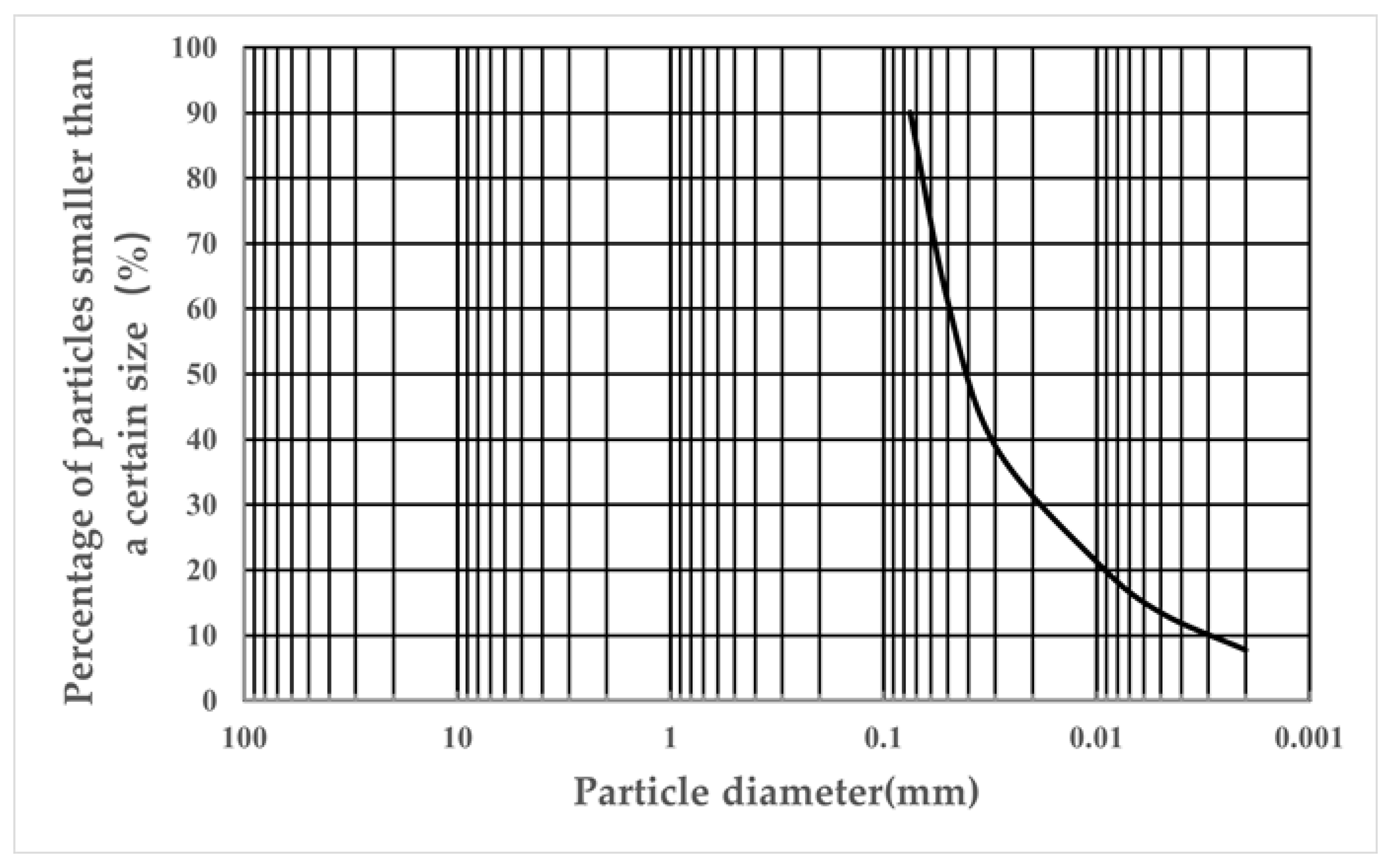
The grain composition of soil samples was determined by sieve analysis and hydrometer (d < 0.075 mm). The results are shown in Table 1 and Figure 3.
Liquid and plastic limit tests were carried out on marine soil samples. The particle size of the soil sample used in the test is less than 0.5 mm, and the combined determination method of liquid and plastic limit is adopted. When the falling cone depth of liquid and plastic limit instrument is 2 mm, the corresponding water content is the plastic limiting water content, and when the falling cone depth is 17 mm, the corresponding water content is the liquid limiting water content. The results are shown in Table 2.
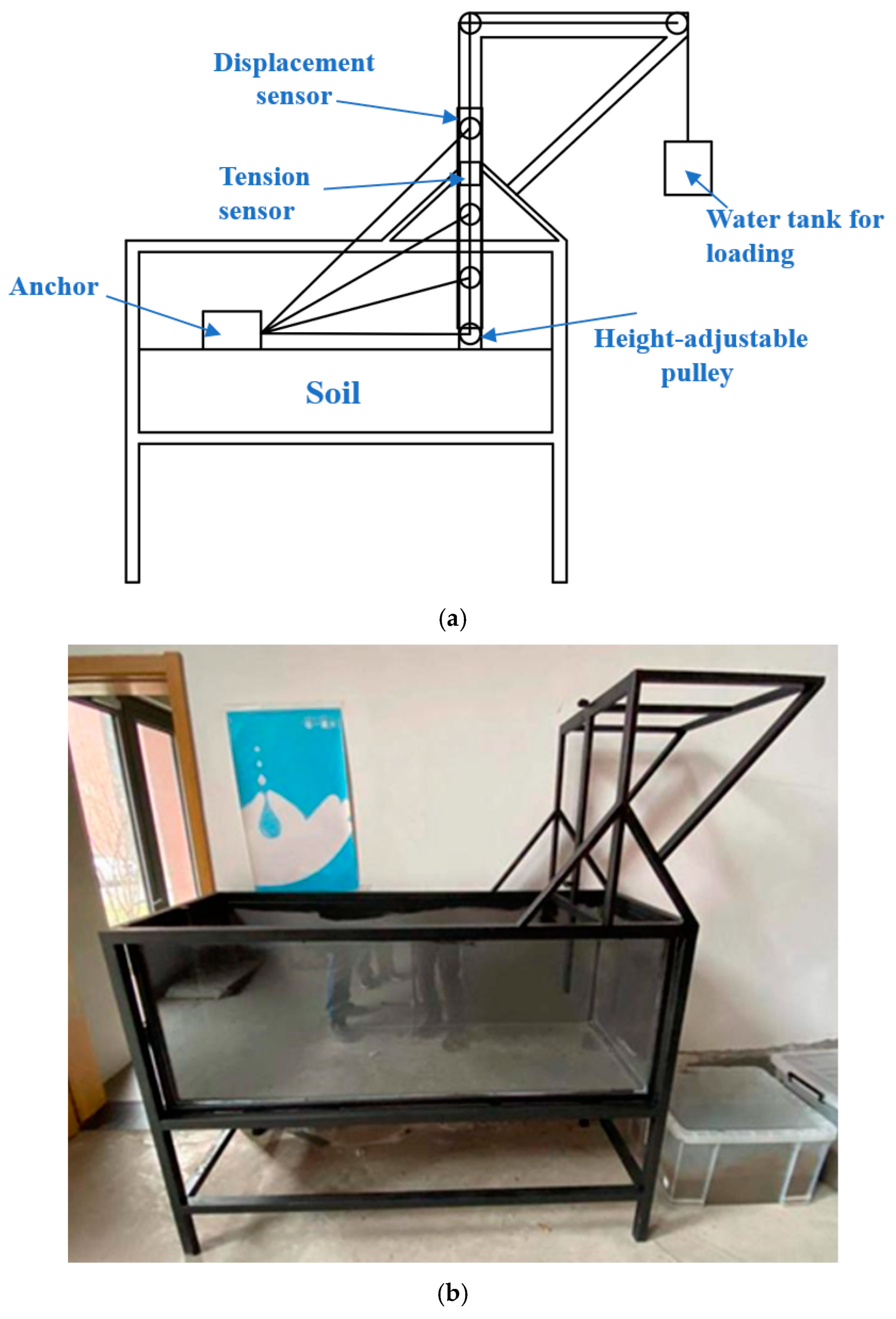
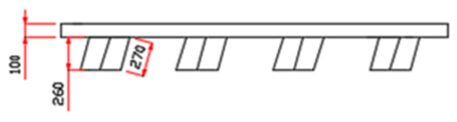
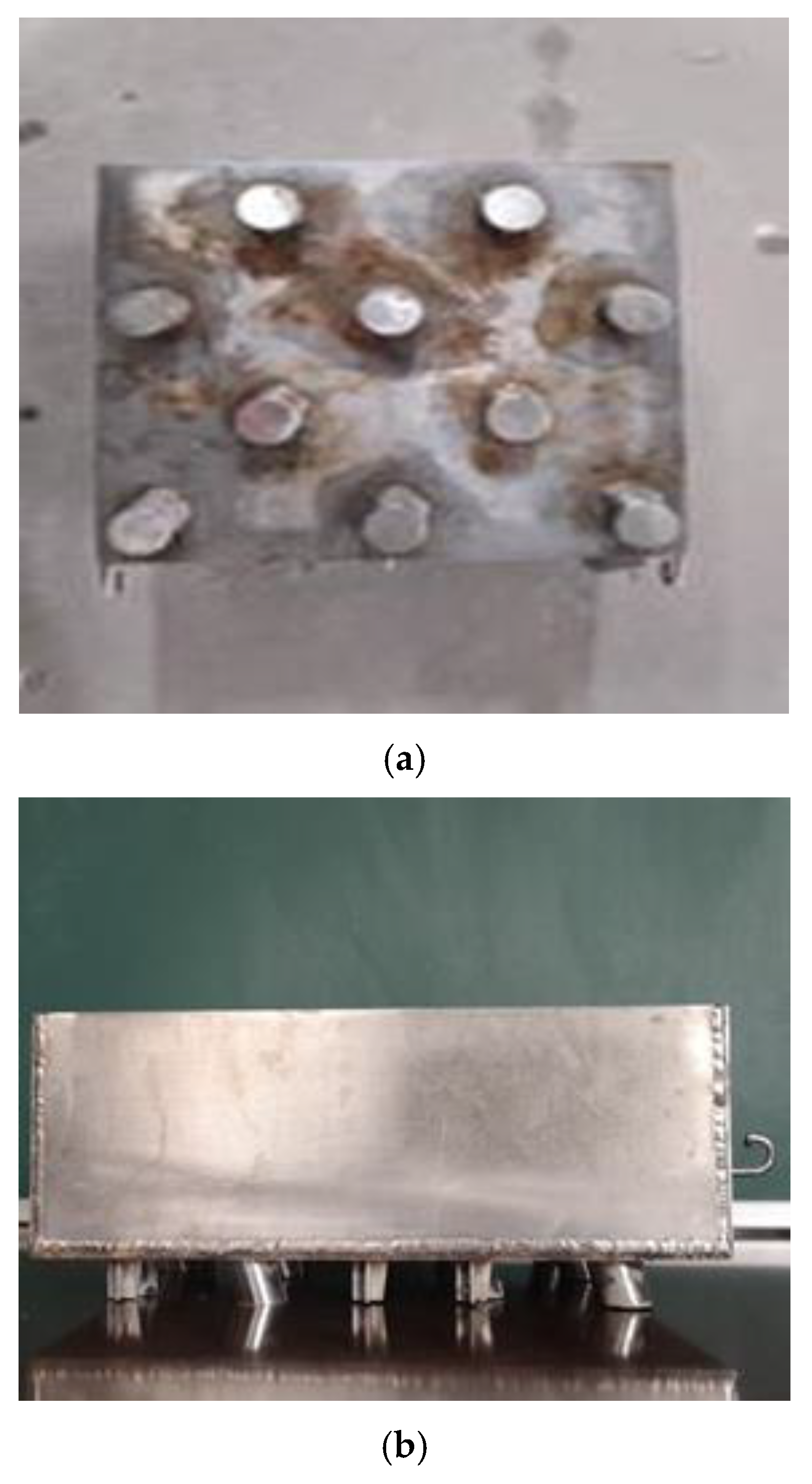
Model tests were conducted in a test tank with a length of 1.75 m, a width of 0.6 m, and a height of 1.2 m, as shown in Figure 4. The height of the soil in the box during the test is 0.3 m. Other soil was laid 0.2 m at the bottom. The total height of the soil is 0.5 m. The height of the soil is 6 times the height of the gravity anchor. The boundary effect can be ignored. The soil is evenly and flatly filled in the test tank. In addition to the test tank, the device is mainly made up of an anchor model (the front, back, and top center are equipped with buckles that can connect to the steel strand), a height-adjustable pulley device, tension, and displacement sensors, and a travel switch (the switch is disconnected and stops loading after the anchor body moves in the model test). The height-adjustable pulley device is used to change the loading angle of the gravity anchor. The model of the tension sensor is TJL-1S, the range is 0~30 kg, and the overall accuracy is 0.02. The model of the displacement sensor is KS20-1000-01-C, the range is 0~1000 mm, and the accuracy is ±0.53%. The shape of the gravity anchor used in the tests is shown in Figure 5 and Figure 6. In this test, the actual gravity anchor of the project is reduced according to the ratio of 1:15. The size of the gravity anchor model in the model test is 200 mm × 200 mm × 87 mm, and the mass is 8.25 kg by using similar criterion. The anchor in the model test was made in advance. The drawing of the anchor in the actual project is shown below. The anchor is hollow and brought to a predetermined weight by adding counterweight blocks in four boxes. The oblique columns at the bottom of the anchor are the shear keys of the gravity anchor. Its function is to increase the contact area with the soil and to change the way the soil fails. These two effects increase the bearing capacity of the gravity anchor. Their exact dimensions are shown below. The height of the shear key is 260 mm, and the length is 270 mm. Its diameter is 300 mm.
Model tests include horizontal loading tests, a series of tests with different loading angles, and vertical loading tests. The angle of the oblique load test remains constant during the test. The test data revealed that the displacement of the gravity anchor was very small when damage to the soil occurred. The displacement of the gravity anchor is negligible in relation to the horizontal distance between the gravity anchor and the displacement gauge. Therefore, the angle of the oblique load test can be considered to remain constant during the test. The load angle was tested during the test. The starting position of the gravity anchor is kept constant in the model test. The force angle can be changed by varying the height of the pulley. Horizontal loading tests are first performed to obtain the load–displacement curve and the failure criteria of displacement. Then, a series of tests with different loading angles and vertical loading tests are performed based on the load-displacement curve during the tests. In the test, the AT-102 model water pump is used to add water to the water tank at a constant speed to load the gravity anchor model. The capacity of the water tank is greater than that required for the maximum test load. The switch is controlled manually. When the pump is turned on, water is poured into the tank. The weight of the injected water in the water tank is applied as a load on the gravity anchor. The loading velocity is 0.3 N/s. Therefore, the strain rate is 1.4 × 10⁻⁴. This entire process can be considered as a quasi-static simulation.
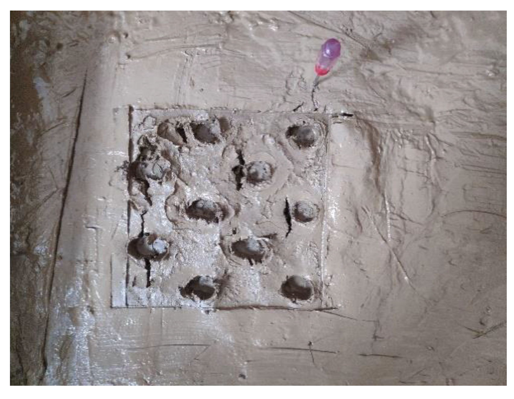
The specific experimental steps are as follows. (1) Gravity anchors are slowly placed in the center of the soil. The gravity anchor is positioned 1 m from the loading end. Additionally, the gravity anchor is positioned in the middle of the test box in the width direction. It is not simply placed on the soil surface. The upper part of the gravity anchor needs to be fitted with counterweight blocks. The aim is to sink the gravity anchor to the preset position. Prior to the start of the model test, the gravity anchor was marked with a marker at the height of 10 cm. When the gravity anchor has settled exactly to the preset depth, the counterweight is removed, and the rest of the operation begins. The tension sensor is connected to the loop on the front end of the gravity anchor. Next, the displacement sensor is installed, and the readings are zeroed. The gravity anchor was left for 10 min to allow the excess pore water pressure of the soil to dissipate. (2) Start recording. Use the water pump to add water to the water tank at a constant speed to load the gravity anchor. (3) When the anchor damages the soil, stop the test. The parallel experiment was repeated 3 times. The tensile force–displacement curve was plotted by taking the average of three parallel tests.
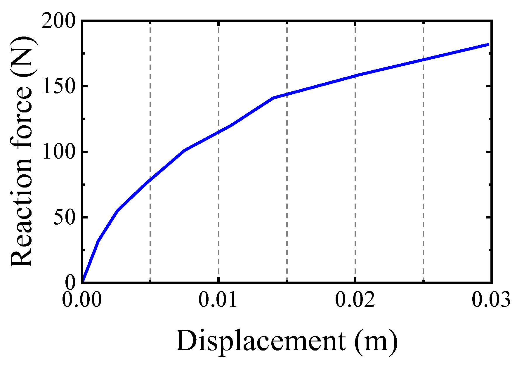
The graph of soil deformation is shown in Figure 7. It can be observed the soil has been destroyed. The load–displacement curve can be obtained by using software to synthesize and process the data collected by the sensor. The load–displacement curve of the anchor under horizontal loads is shown in Figure 8. The load carrying capacity of a gravity anchor is the maximum force that can be provided by the gravity anchor while the anchor remains stable and does not break the soil. When the gravity anchor moves to the distance of 0.01 m, the soil has been damaged, at which point the corresponding force is the gravity anchor bearing capacity.
In clay, the formula for calculating bearing capacity is written as:
where and represent horizontal bearing capacity and undrained shear strength of soil at depth , is the average undrained shear strength of the soil from anchor bottom to the depth , is the area of anchor bottom, is the depth of anchor burial, is the width of the anchor bottom, is the bulk density of the soil.
The parameters in Equation (1) are determined according to the size of the anchor in the model test, the embedded depth, and the strength of the soil. The ultimate bearing capacity were determined according to Equation (1), and the model test results are 379.5 kN and 421.9 kN. The test results are in good agreement with the calculation results based on the theoretical formula, and the difference between the two is about 10%.
3. Numerical Simulation of Gravity Anchors
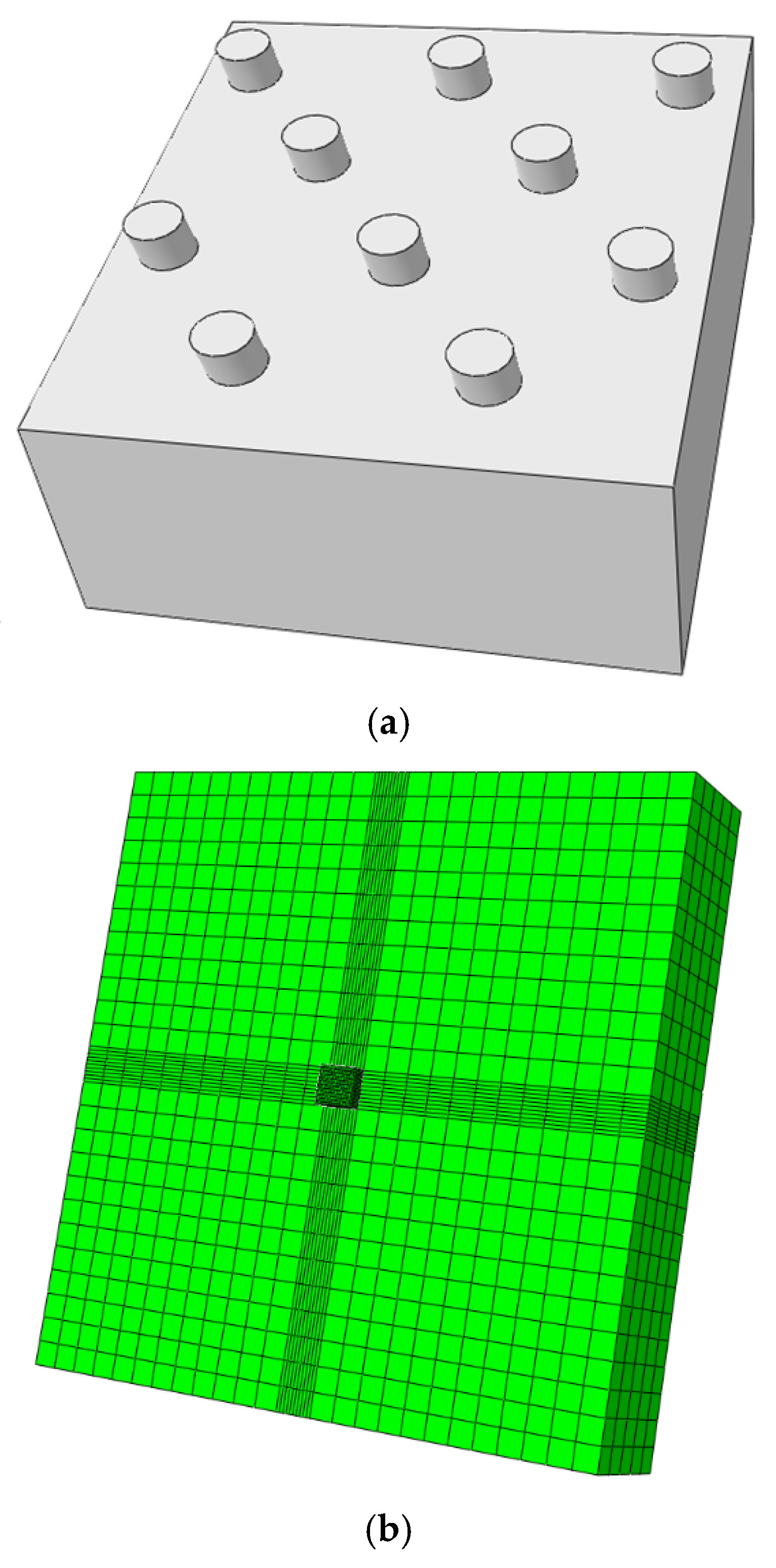
To analyze horizontal bearing mechanism of the gravity anchor, the finite element method is used to analyze the gravity anchor. The model was established based on the ABAQUS software, according to the specific dimensions of the model anchor, the size of the soil domain in the model test tank, and the boundary conditions. The length and width of the gravity anchor are both 3 m, the height is 1.3 m, the weight is 80 tons, and the floating density in seawater is 5812.6 kg/m3. The material of the gravity anchor is steel. The elastic modulus is 210 GPa, and the Poisson’s ratio is 0.3. The 3D finite element model of gravity anchor is shown in Figure 9a. The gravity anchor has 10 column bases. The height of the shear key is 260 mm and the length is 270 mm. Its diameter is 300 mm. Shear keys are evenly distributed at the bottom of the gravity anchor. The calculation range of the soil body is determined according to the outer dimensions of the anchor body. To eliminate the influence of the boundary, the depth and width of the soil are both about 5 times the corresponding height and width of the anchor. Therefore, the size of the soil model is 50 × 50 × 10 m. The 3D finite element model of soil is shown in Figure 9b.
Normal horizontal constraints are applied to the vertical boundaries, and fixed constraints are applied to the bottom boundary. The top boundary is fully free. The gravity anchor model is not constrained and can move freely. The anchor is treated as a rigid body during calculations. The frictional contact is set between the model anchor and the surrounding soil. The surface of the anchor is set as a master surface, and the surface of the soil in contact with it is set as a slave surface. Separation is allowed in the normal direction of the contact surface. When the gravity anchor bears the horizontal load, the Coulomb friction contact is set between the anchor and the soil. The friction force on the contact surface of the anchor and soil is related to the normal force between the contact surface of the anchor and soil. When the gravity anchor bears an inclined load, the critical shear stress friction contact between the anchor and the soil is set. The tangential slip condition is considered to only be related to the critical shear stress. When the shear stress between the anchor–soil interface is less than the critical shear stress, the anchor and the soil are in a state of mutual bonding without relative slip; on the contrary, the anchor and the soil produce relative slip. The critical shear stress is represented by Equation (2).
where is the critical shear stress; is cohesion coefficient; is undrained shear strength.
Hexahedral elements are used to divide the soil into grids, and tetrahedral elements are used to divide the gravity anchors into grids. To improve the simulation accuracy, the soil unit is divided into units by progressive encryption, as shown in Figure 9b. Mesh smoothing is used in the calculation process. Mesh smoothing is to smooth the deformed mesh without changing the connections among mesh nodes.
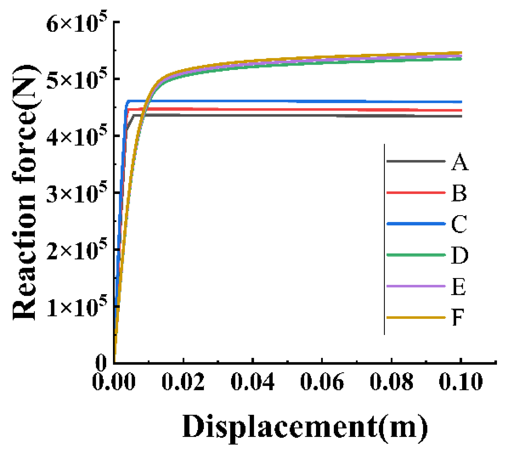
The contact parts of gravity anchor and soil are divided into different grids to study the grid sensitivity. The unit division is shown in the following table. When the grid number is less than 10 × 10, soil failure occurs earlier. Gravity anchors also have less carrying capacity. Therefore, the grid precision is not enough. When the grid number is greater than 10 × 10, the bearing capacity curve is basically unchanged. Considering the computational efficiency, it is better to choose a 10 × 10 grid number. The results are shown in Table 3 and Figure 10.
The density of soil is 1800 kg/m3. The floating density is 800 kg/m3. Poisson’s ratio is 0.45. Additionally, the elastic modulus is 5 MPa. The soil plastic model is the Mohr–Coulomb plastic model. The expansion angle is 0.25, and the cohesion is 10 kPa. The behaviors of the gravity anchors were analyzed by the finite element method according to three steps. (1) Geostatic: In this step, the initial ground stress of the soil is balanced so that the initial displacement of the soil is zero. (2) Contact: The purpose of this step is to establish contact between the anchor and the soil. (During the modeling process, it was assumed that the contact time between the anchor and soil was long enough at the second analysis step to ignore pore water pressure. At this point, pore water pressure is considered to have completely dissipated.) (3) Load: Load the gravity anchor to move it at this step.
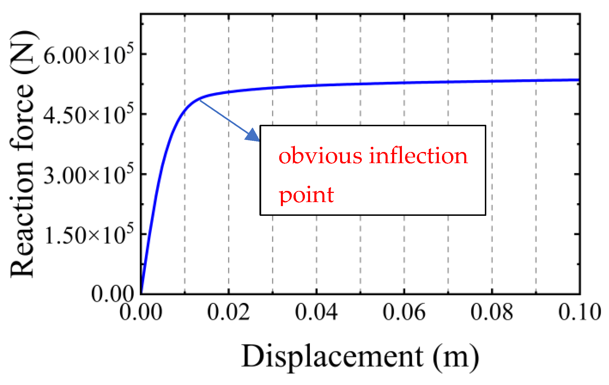
Apply loads to the model and run the software. The curves of horizontal bearing capacity and horizontal displacement are extracted to draw the image shown in Figure 11. It can be found that the curve has a more obvious inflection point. The ultimate bearing capacity of the gravity anchor is generated here. The soil is destroyed at this point. The corresponding ordinate is the horizontal bearing capacity of the gravity anchor. The result of numerical simulation is 455.7 kN, with an error of 8% after comparison with the model test. The predictions are generally in agreement with the test results, which indicate the plastic strain accumulation characteristics of the soft clay surrounding the anchor can be captured by the finite element method. So, the simulation results are considered correct and can be used for comparative analysis.
4. Results and Discussion
4.1. Mechanism of Sliding and Bearing Capacity of Gravity Anchor in Clay
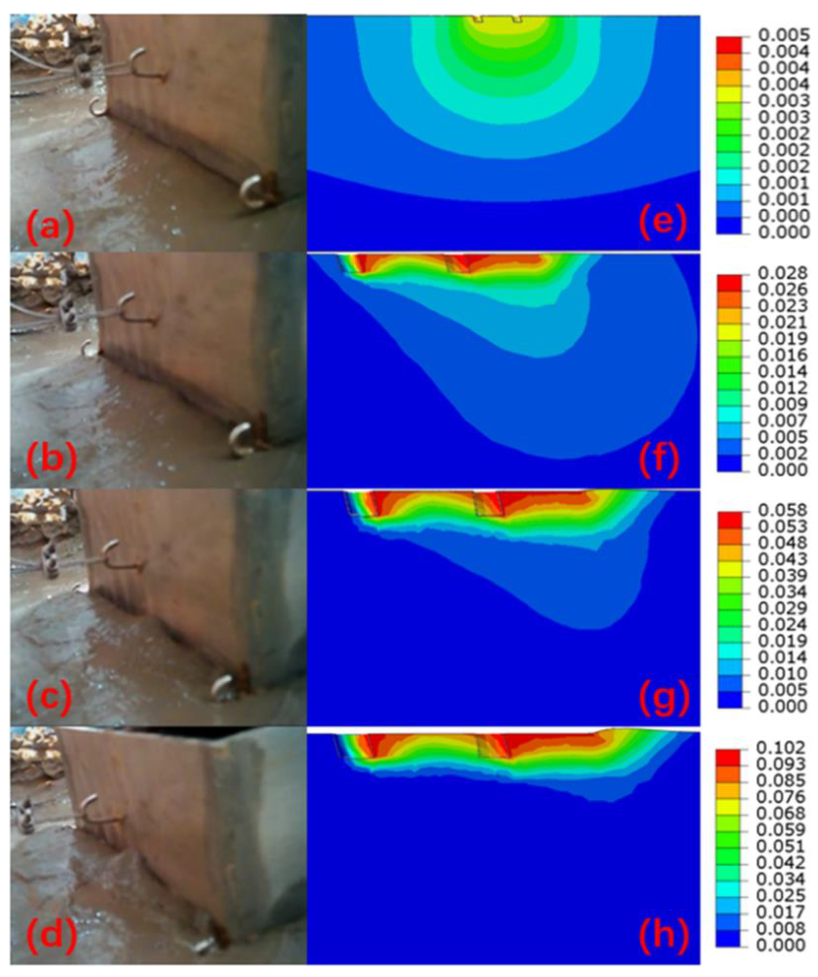
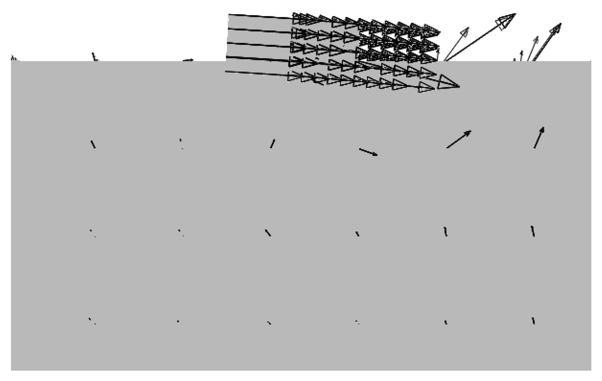
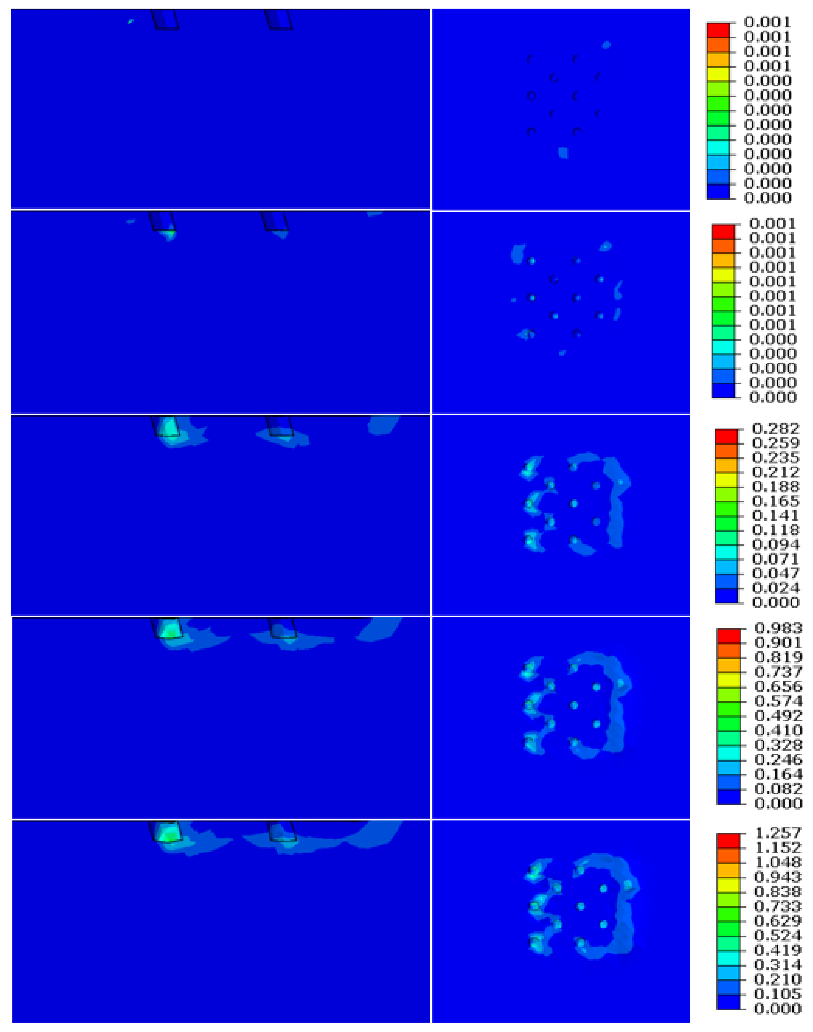
It follows from the obtained capacity–displacement curve that the gravity anchor moves under horizontal tension in the clay. The bearing capacity tends to reach the maximum when the sliding preventer force is gradually increased to a certain level. So, the type of soil destruction is progressive destruction [26]. Sliding of the anchor occurs inside the soil, as shown in Figure 12. Figure 12 presents the deformation of the clay layer and the motion of the gravity anchor. As the displacement of the gravity anchor increases, the area and size of the soil deformation increase. The results of the model test and numerical simulations are in good agreement. The results in the figure show that the amount of soil deformation gradually increases with the motion of the gravity anchor. The settlement of the front part of the gravity anchor is larger than that of the back part. In other words, the gravity anchor will settle during the motion of the gravity anchor. The gravity anchor is a forward-tilted settlement. This is due to the fact that to balance the tensile moment, the soil body needs to provide a large vertical stress. It is accompanied by a large settlement of the front end of the soil mass. Liang J and Song X proposed that the soil in front of the anchor was formed due to the horizontal motion of soil particles. However, through the study presented in this paper, it was found that the soil in the passive zone in front of the anchor is squeezed during the tilted motion of the anchor. Due to the partially fluid nature of the clay, the clay at the bottom of the anchor will flow as it is squeezed by the gravity anchor. When a surge occurs, the forward body of the soil will move upwards after being squeezed by the clay at the bottom of the anchor. Finally, the phenomenon of soil accumulation at the front end of the anchor is formed. This is also verified in Figure 13. The displacement vector of soil indicates that accumulation of soil occurs in front of the soil. The gravity anchor is inserted into the soil. As a result, the soil in front of the gravity anchor flows and accumulates in front of the gravity anchor.
The front soil is actively damaged by gravity anchors and is greatly deformed. The soil area behind the anchor is passive. The posterior soil is not affected by the gravity anchor. However, it can be seen from the figure that there are some deformations. This is due to the fact that the soil area at the rear end of the anchor flows as the anchor moves, and its settling and deformation is caused by its gravity. During the motion of the gravity anchor, soil deformation is concentrated around the gravity anchor. The deformation of the soil close to the gravity anchor is larger than the deformation of the soil away from the gravity anchor. The closer the soil is to the anchor, the greater the deformation. It can be seen from the Figure 14 that the plastic deformation of the soil first occurs in two small areas around the anchor. At this time, the plastic deformation is relatively small. This is caused by the gravity of the gravity anchor. As the motion process progresses, the soil around the shear key at the rear of the anchor first appears plastically deformed. So, the failure of the soil starts from the rear shear key. The soil in front of the anchor immediately undergoes plastic deformation and failure. Along with the motion of the anchor, the front shear key gradually begins to destroy the soil. Additionally, the damage extends to the soil surface. As a result, the destruction of soil is a gradual process. The plastic deformation of the soil is mainly concentrated near the shear key and around the anchor. Gravity anchors locally damage the soil during motion and then reach the ultimate bearing capacity. So, the failure mechanism of the soil is a local failure. In summary, the failure mechanism of soil mass is a local progressive failure.
4.2. Analysis of Influencing Factors of Gravity Anchor Bearing Capacity in Clay
4.2.1. Influence of Clay Properties on Bearing Capacity of Gravity Anchor
From the above analysis, it is clear that the type of soil destruction is progressive destruction and that the sliding of the anchor occurs inside the soil. Thus, the properties of the clay have a large impact on the bearing capacity of the gravity anchor. Furthermore, the influence of the friction angle and cohesion of the clay on the bearing capacity of the gravity anchor is investigated.
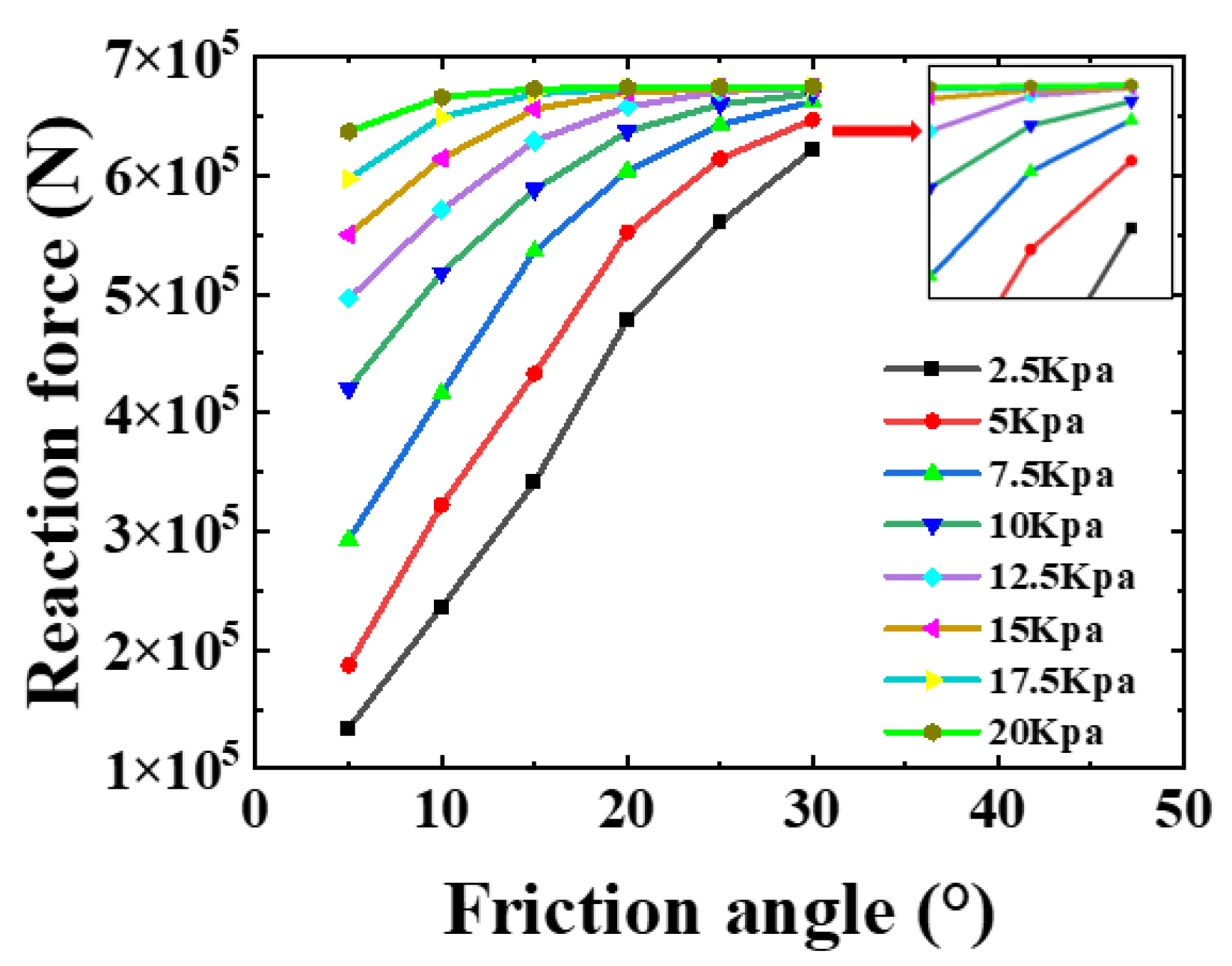
A 3 × 3 × 1.3 m gravity anchor model was established to study the influence of clay properties on bearing capacity. First, we changed the friction angle to study the effect of friction angle on the bearing capacity. From Figure 15, it can be found that with the increase in friction angle, the bearing capacity shows an increasing trend. The bearing capacity changes obviously when the friction angle is small. However, when the friction angle increases to 30 degrees, the change in bearing capacity tends to be stable. From the enlarged view of the end curve, it can be known the bearing capacity curves of 12.5 kPa–20 kPa coincide when the friction angle is 30 degrees. The bearing capacity reaches a fixed value, and the size of the value is 675,000 N. When the cohesion is less than 12.5 kPa, the bearing capacity increases to a greater extent with the increase in the friction angle. However, the tendency of bearing capacity to change with friction angle is small after cohesion exceeds 12.5 kPa. Therefore, as the cohesion increases, the effect of the friction angle on the bearing capacity decreases gradually.
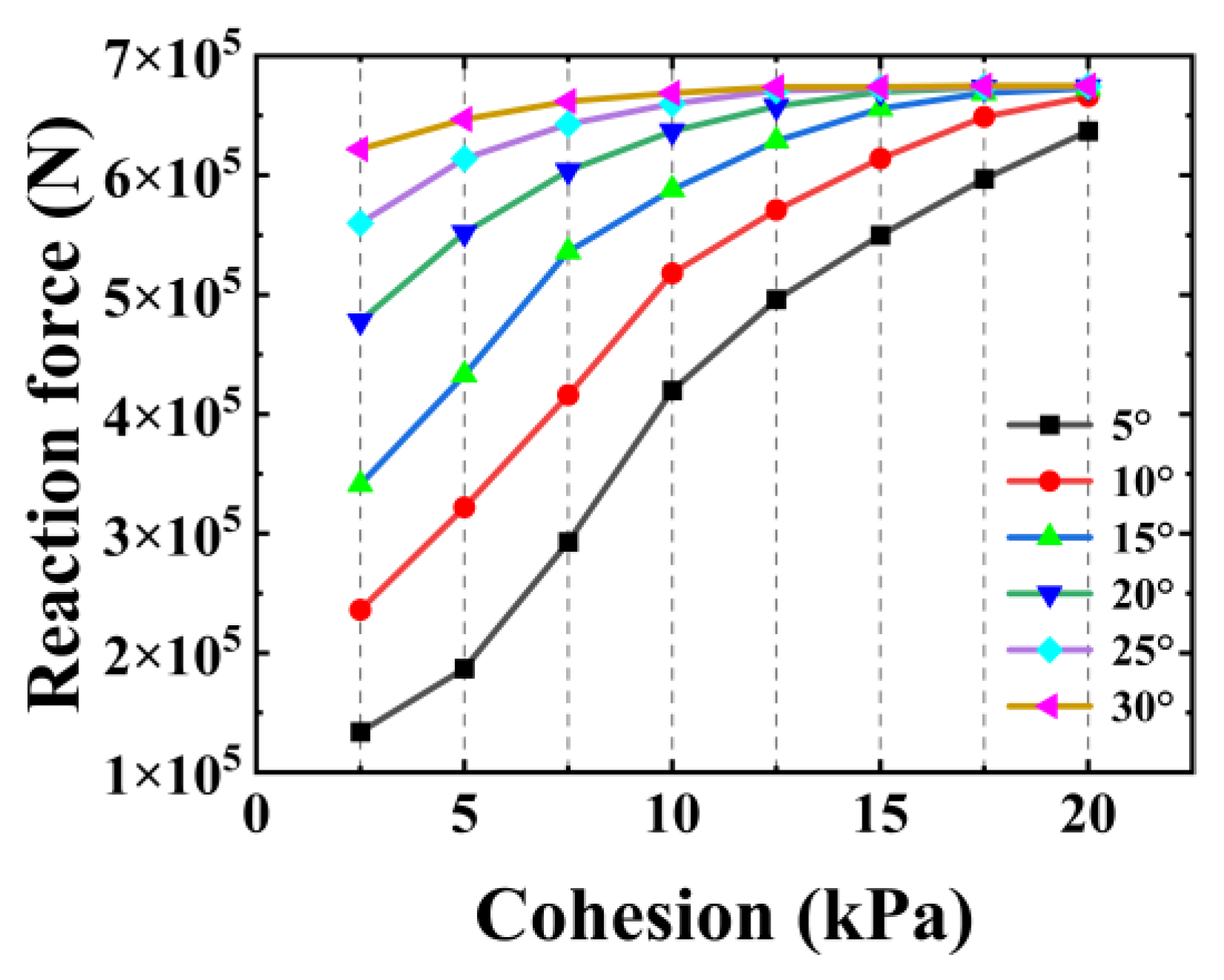
The cohesion was changed to obtain the bearing capacity curve, as shown in Figure 16. As the cohesion increases, the bearing capacity also shows an increasing trend. Additionally, with the increase in cohesion, the change in the bearing capacity curve gradually becomes gentle. It can be seen from the figure that the initial value of each bearing capacity curve increases with the increase in the friction angle. When the friction angle gradually increases to a certain value, the bearing capacity tends to remain at a certain fixed range. Therefore, as the cohesion increases, the bearing capacity curve tends to be flat. The increase in the friction angle has less and less influence on the bearing capacity.
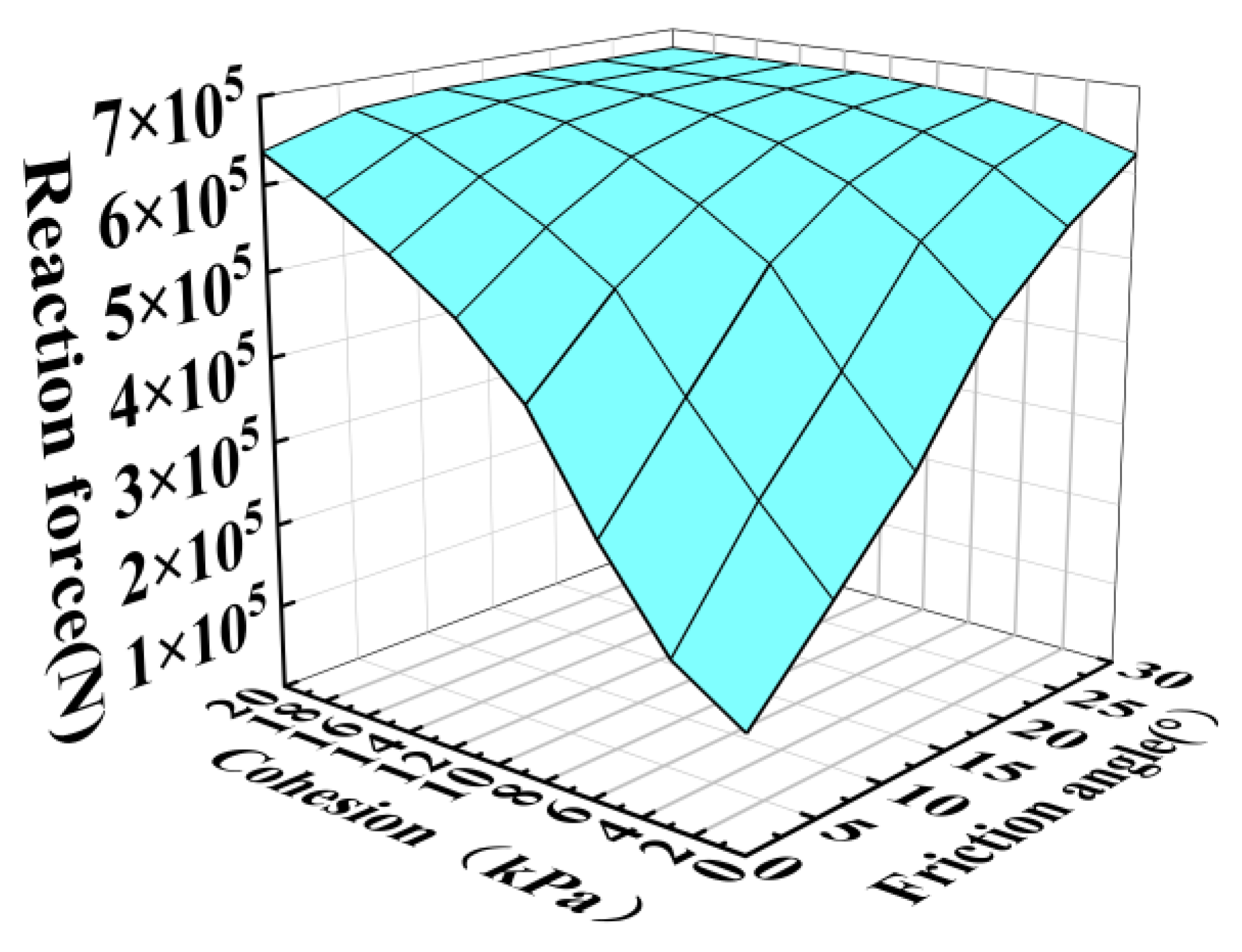
The effects of friction angle and cohesion on the change in bearing capacity are plotted on a 3D surface plot, as shown in Figure 17. The part where the surface changes greatly is concentrated on the front side. In the range where the cohesion is less than 12.5 kPa and the friction angle is less than 15°, the bearing capacity varies greatly from 134,000 N to 629,000 N. The central slope of the surface change is 2.53. When the cohesion exceeds 12.5 kPa and the friction angle exceeds 15°, the change in the bearing capacity is small. The bearing capacity varies from 629,000 N to 675,000 N. The central slope of the surface change is 0.51. In this range, the change of cohesion and friction angle has little effect on the bearing capacity. The bearing capacity gradually becomes stable. Therefore, the bearing capacity of the gravity anchor is limited and cannot be increased indefinitely with the change of clay parameters. The bearing capacity of gravity anchors changes significantly when the clay parameters are low. When the clay parameters increase to a certain extent, since the weight of the gravity anchor does not change, the bearing capacity is limited by its weight and gradually reaches the maximum bearing capacity.
4.2.2. Influence of Gravity Anchor Bottom Area and Mooring Point Height on Bearing Capacity of Gravity Anchor
The bearing capacity of gravity anchors is mainly provided by the friction between the anchor bottom and the soil. The damage is mainly the sliding damage of the anchor bottom and the soil. The main factors affecting the friction force are the positive pressure at the bottom of the anchor and the contact area between the bottom of the anchor and the soil (i.e., the coefficient of sliding friction). When the gravity of the anchor is constant, the anchor volume is constant. When the area of the anchor bottom is changed, the vertical pressure of the anchor bottom and the contact area with the soil is changed at the same time. Therefore, the product of the two must have a maximum value. We kept other parameters unchanged and only changed the size of the anchor bottom area to study the influence of the anchor bottom area on the bearing capacity of the gravity anchor.
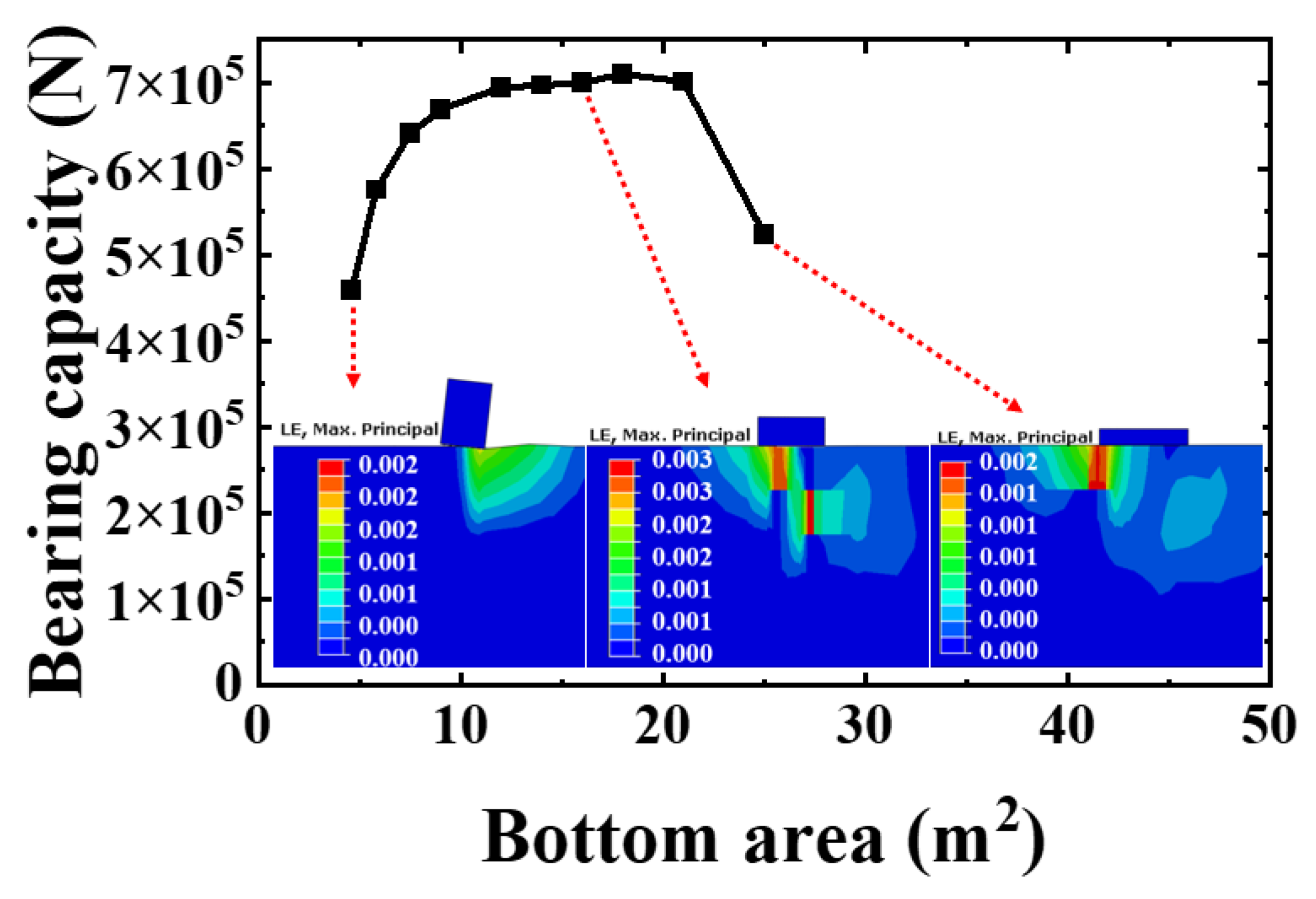
From Figure 18, it can be found that there is an optimal bottom area for the gravity anchor. When the area is less than the optimal area, the bearing capacity increases from 459,186 N to 710,181 N. The increase ratio is 54.7%. When the bottom area is larger than the optimal area, the bearing capacity is reduced from 710,181 N to 522,911 N. The reduction ratio is 26.4%. The soil true strain maps of gravity anchors, as shown in Figure 18, with bottom areas of 4 m2, 9 m2, and 16 m2 are extracted to study the reasons for the change in bearing capacity. It is obvious that the soil mass with the optimal bottom area has the largest true strain. Additionally, the deformation area of the soil is the largest. The depth of the impact of gravity anchors on the soil is also the largest. For gravity anchors whose bottom area is less than the optimal area, the soil strain is the largest below the front edge of the anchor bottom. Therefore, the failure of the bearing capacity is mainly caused by the local failure of the soil at the front of the anchor bottom. The maximum soil strain of the gravity anchor with the bottom area larger than the optimum area appears on the surface of the subsoil. The failure of the bearing capacity is mainly caused by the damage to the surface soil at the bottom of the anchor. However, the maximum soil strain of the gravity anchor with the optimal area appears in the deep layer of the soil. The failure of the bearing capacity is mainly caused by the overall failure of the anchor bottom soil. Therefore, when the anchor bottom area is less than the optimal area, the soil failure is a local failure. When the anchor bottom area is larger than the optimal area, the soil failure is the sliding failure of the shallow layer. When the anchor bottom area is the optimal area, the soil failure is a deep failure. Therefore, the bearing capacity of the gravity anchor with the optimal area is the largest.
It can be seen the optimal area is around 18 m2. So, the optimal size is 4.3 × 4.3 × 0.633 m. According to the specification, it can be calculated that the minimum width of the anchor bottom is 2.40 m. Therefore, the finite element calculation results are within the range of the formula calculation results. It can be seen from Table 4 that when the anchor bottom area is in the range of 11–18 m2, the horizontal bearing capacity varies little. The shapes of the bottom surfaces of the anchors studied above are all squares. In the following, rectangles with different lengths and widths, which have the same bottom area (9 m2), are used to study the influence of the bottom shape on the bearing capacity. The calculation results are shown in Table 4. It can be found from Table 1 that the shape of the anchor bottom has little effect on the horizontal bearing capacity. The horizontal bearing capacity corresponding to the square section is slightly higher than that of the rectangular section. Therefore, a square anchor base shape is slightly better than a rectangle.
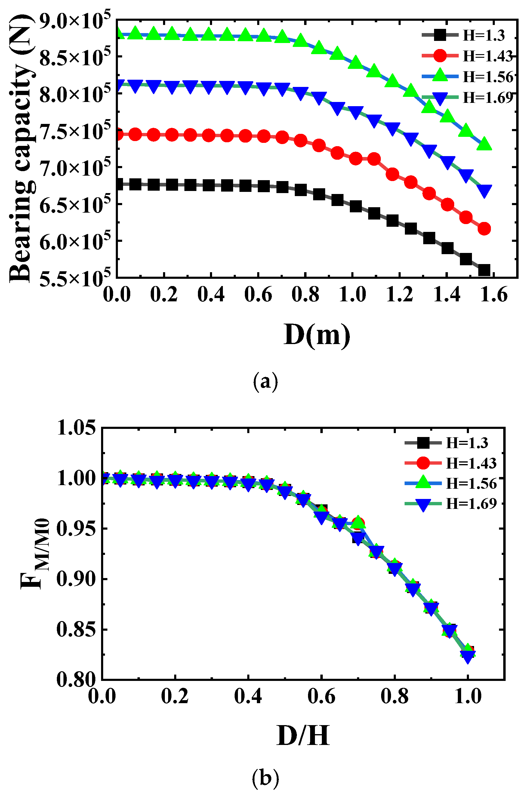
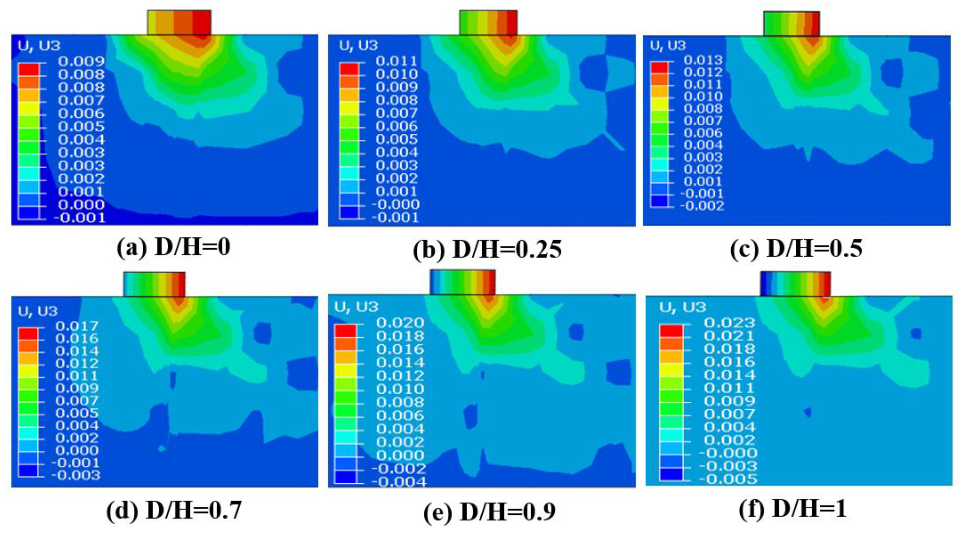
The location of the gravity anchor mooring point is closely related to the bearing capacity of the gravity anchor. The bearing capacity of the same gravity anchor at different mooring heights is obtained by using gravity anchor models. The calculation results are shown in Figure 19a. In each group of models, the bearing capacity of the gravity anchor decreases with the increase in mooring point height. The change trends of each group of curves in the figure are similar. The bearing capacity of the first half of the curve decreases slightly, and it can be considered that there is no change in the first half. The bearing capacity of the second half of the curve decreases greatly. In this part, the bearing capacity is greatly affected by the mooring height. It can be clearly found from Figure 20 that when 0 < D/H < 0.5, the vertical displacement of the gravity anchor changes very little. The vertical displacement of the gravity anchor increases by a factor of 2 when D/H is between 0.5 and 1. The gravity anchor has undergone a relatively obvious flip in this interval. Stability and carrying capacity are greatly reduced. When the height of the mooring point of the gravity anchor is less than 0.5 H, the gravity anchor only translates and does not rotate under the action of tension. However, when the height of the mooring point exceeds 0.5 H, the gravity anchor will rotate. The bearing capacity of the gravity anchor will gradually decrease. The higher the height of the mooring point, the greater the rotation amplitude and the smaller the carrying capacity.
Dimensionless processing is performed on the data in Figure 19a to obtain the dimensionless relationship between the height of the mooring point and the bearing capacity, as shown in Figure 19b. Dimensionless bearing capacity (FM/M0) is the ratio of real-time bearing capacity (FM) to ultimate bearing capacity (FM0). Dimensionless altitude (D/H) is the ratio of real-time altitude (D) to maximum altitude (H). It can be found from the figure that the dimensionless curves of gravity anchors with different heights and weights coincide. This shows that height and weight do not affect this relationship. As the height of the mooring point increases, the rate of decrease in the bearing capacity also increases. The curve can provide a reference for engineering practice and estimate the influence of the mooring point height on the bearing capacity of gravity anchors. For the convenience of this research, the fitting formula (3) is obtained by fitting the trend curve. The fitting coefficient is R2 = 0.99088.
The above formula can be used to estimate the influence of the height of the mooring point on the bearing capacity. When the dimensionless height increases to 0.7, the dimensionless bearing capacity drops to 0.95. While the dimensionless height increases from 0.7 to 1, the dimensionless bearing capacity drops to 0.82. The dimensionless bearing capacity decreased by 0.13 in this interval, indicating that the increase in height has a greater negative impact on bearing capacity in this interval. Therefore, it is suggested that the design height of the mooring point of the gravity anchor should not exceed 0.7 of the total height. In practical engineering, it is necessary to calculate the anti-overturning moment according to different anchor weights to ensure that gravity anchors will not overturn. Therefore, the value of D/H in actual engineering also needs to calculate the overturning moment to ensure the stability of the gravity anchor.
4.3. Influence of the Height of the Mooring Point on the V-H Failure Envelope Curve
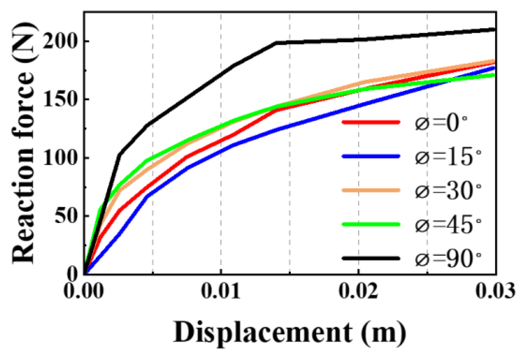
The gravity anchor model test rig mentioned in Section 2 has a height-adjustable pulley. The force angle of the anchor can be changed by adjusting the height of the pulley. We adjusted the pulley height to test and obtain the experimental data presented in Figure 21. The figure shows the bearing capacity–displacement curves of the force angles of 0°, 15°, 30°, 45°, and 90°, respectively.
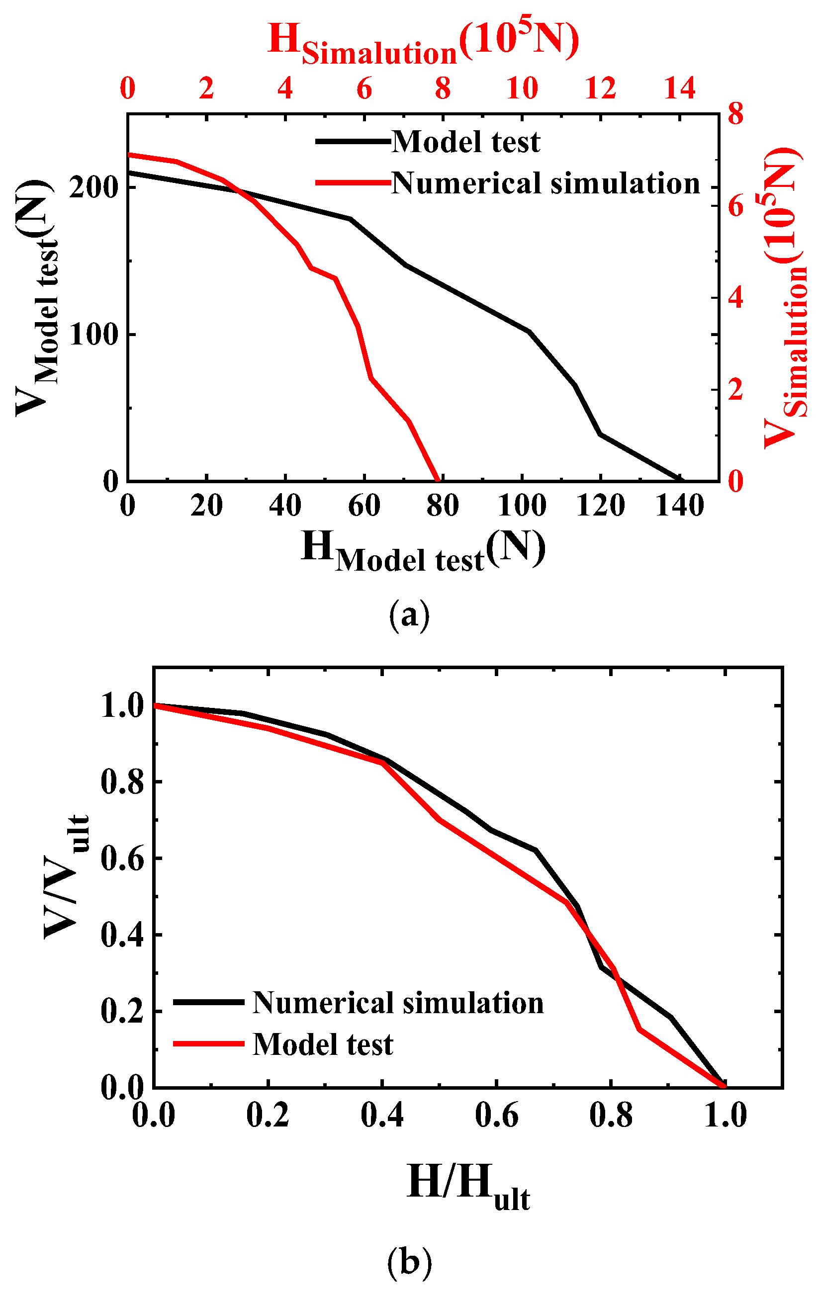
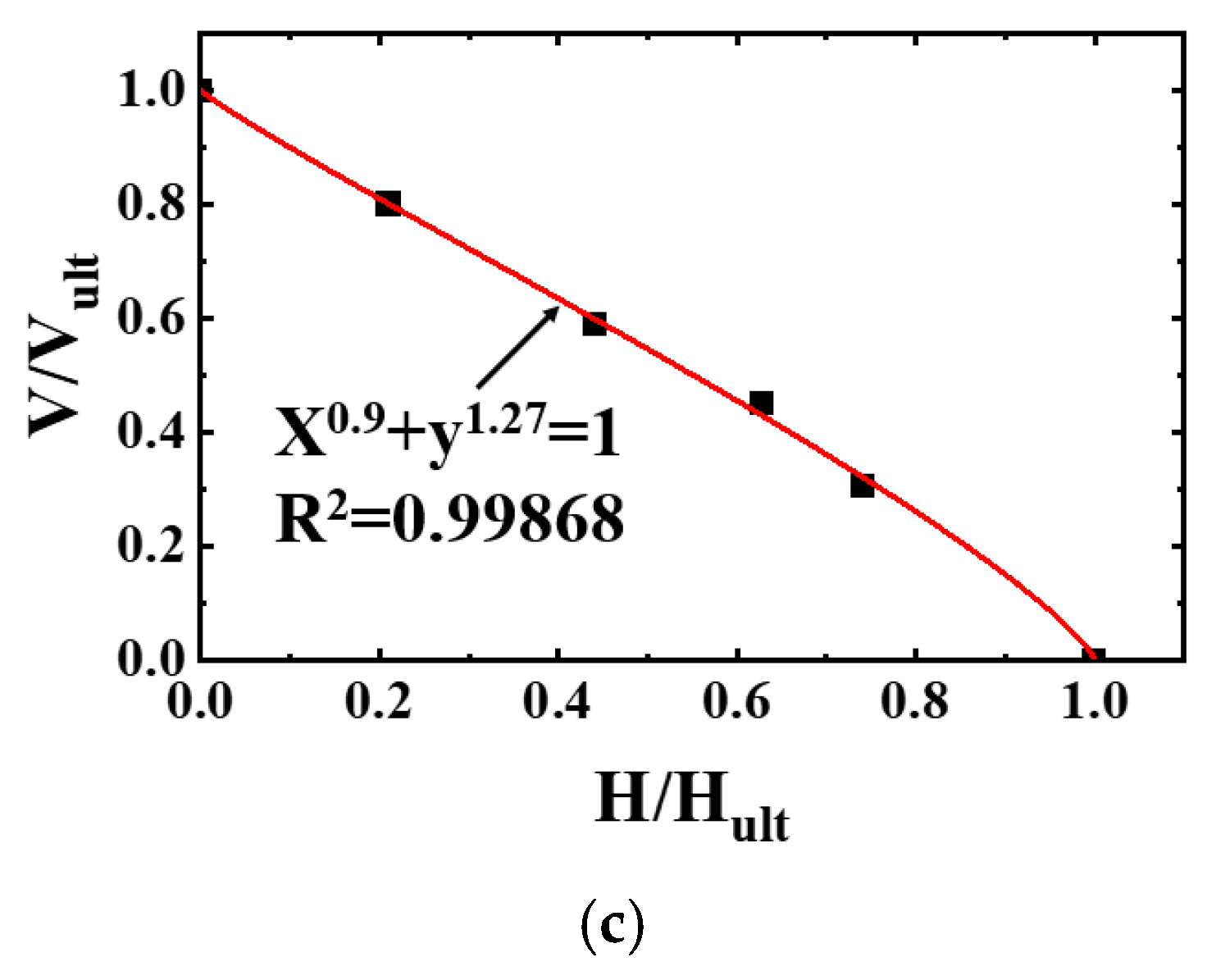
The V-H failure envelope is an effective way to reasonably express the ultimate bearing capacity of shallow buried foundations. The V-H envelope of the model test is plotted in Figure 22a. Hsimalution represents the horizontal bearing capacity results in the numerical simulation. HModel represents the horizontal bearing capacity results in the model test. Vsimalution represents the vertical bearing capacity results in the numerical simulation. VModel represents the vertical bearing capacity results in the model test. The black curve and axis in the figure represent the failure envelope of the model test. The V-H failure envelope of the same gravity anchor is drawn by finite element modeling, as shown in Figure 22a. The red curves and axes in the figure represent the numerically simulated failure envelopes. The V-H failure envelopes of numerical simulations and model tests are normalized. The results are shown in Figure 22b. Hult represents the maximum horizontal load carrying capacity. Additionally, Vult represents the maximum vertical load capacity. From the figure, it can be found that the normalized V-H failure envelopes of the numerical simulation and the model test coincide. So, the results of the numerical simulation can be used for analysis.
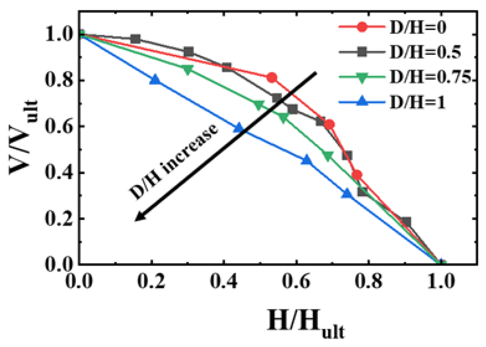
Next, the influence of the gravity anchor mooring point height on the V-H failure envelope is studied. The bearing capacity is obtained by changing the height of the mooring point of the gravity anchor. We plotted the normalized V-H failure envelopes for different D/H (D represents the gravity anchor mooring point height, and H represents the gravity anchor height), as shown in Figure 23. It can be known from the figure that the normalized V-H failure envelopes of gravity anchor foundations with different mooring heights are similar. However, as the mooring height increases, the failure envelope gradually shrinks inward. When the horizontal bearing capacity generated by the inclined load is less than 20% of the ultimate horizontal bearing capacity, the normalized vertical load of the anchor changes little. When the horizontal bearing capacity exceeds 20% of the ultimate horizontal bearing capacity, the normalized vertical load varies greatly.
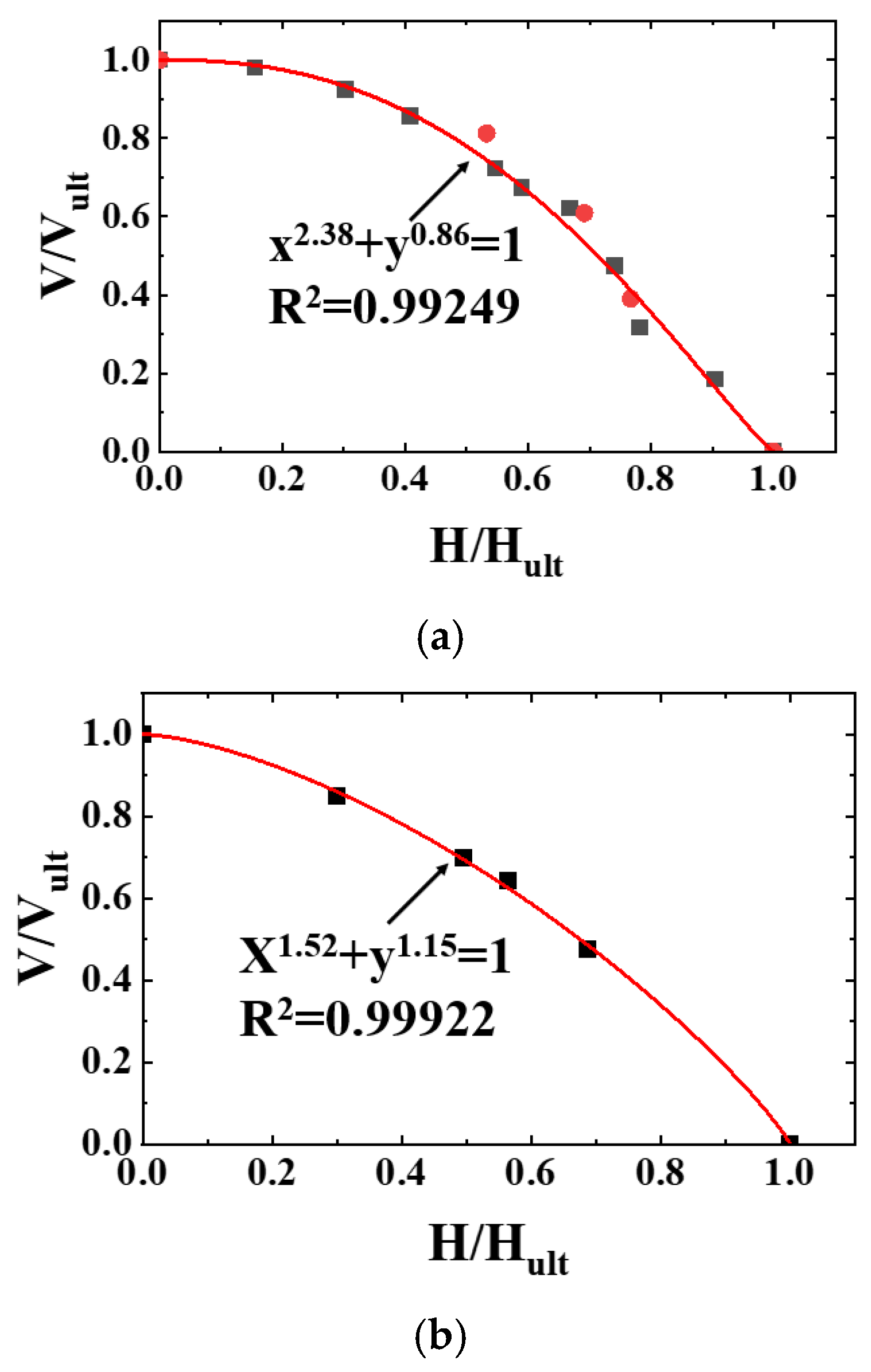
Furthermore, the mathematical expression of the normalized V-H failure envelope is obtained by studying the variation law of the normalized V-H failure envelope at different mooring heights. Bransby and Randolph [27] proposed a normalized failure envelope formula in the V-H stress space for shallow buried foundations.
Zdravkovic et al. [28] suggested that the values of a and b should be a = b = 2 when the anchor foundation with a length-to-diameter ratio L/Di = 0.5~1.4 is under an inclined load. Senders and Kay [29] suggested that the values of a and b should be a = b = 3 when the anchor foundation with a length-to-diameter ratio L/Di = 2.8 is under an inclined load. Many scholars have fitted the normalized failure envelope in the V-H stress space with mathematical expressions to study the values of a and b. However, the change in the height of the mooring point was not considered. Based on the content of this section, the fitting curve is obtained by fitting the above normalized V-H failure envelope. The fitting results are shown in Figure 24.
From the fitting result of the normalized failure envelope of the V-H stress space, the mathematical expression formula considering the height of the mooring point can be obtained as:
5. Conclusions
The motion behavior of gravity anchors under different angular loads is investigated by conducting model tests. Then, the bearing capacity of gravity anchors in soft clays is simulated using the finite element method based on the ABAQUS software package. The key conclusions can be summarized as follows:
- (1)
- The type of soil destruction is progressive destruction during the movement of the gravity anchor. The damaged area of the soil is mainly concentrated near the gravity anchor. Additionally, the failure mechanism of the soil is a local failure.
- (2)
- With the increase in friction angle and cohesion, the bearing capacity shows an increasing trend. The bearing capacity changes obviously when the friction angle and cohesion are small. However, when the friction angle and cohesion increase to a certain value, the change in bearing capacity tends to be stable.
- (3)
- Gravity anchors have an optimal bottom area with the largest bearing capacity. When the bottom area is determined, the shape of the bottom surface has little effect on the bearing capacity.
- (4)
- When the height of the mooring point is below 0.5 H, the bearing capacity of the gravity anchor is unaffected. As long as it exceeds 0.5 H, the bearing capacity of the gravity anchor decreases immediately. The normalized V-H failure envelopes of gravity anchor foundations with different mooring heights are similar. However, as the mooring height increases, the damaged envelope gradually shrinks inward.
The limitation of this study is that it only considers the bearing state of gravity anchors under a static state. The process of gravity anchor bearing under dynamic conditions was not studied further. In the future, centrifuge will be used to study the bearing process and ultimate bearing capacity of gravity anchors under dynamic conditions.
Author Contributions
Conceptualization, Y.Y. and P.L.; methodology, P.L. and J.Y.; software, P.L.; validation, P.L. and X.L.; formal analysis, P.L. and X.L.; investigation, P.L. and H.L.; resources, Y.Y. and P.L.; data curation, P.L. and X.Z.; writing—original draft preparation, P.L.; writing—review and editing, P.L.; visualization, R.S.; supervision, Y.Y.; project administration, J.Y.; funding acquisition, J.Y. All authors have read and agreed to the published version of the manuscript.
Funding
This research was funded by The National Natural Science Foundation of China (Grant No. 51879189) and National Natural Science Foundation of China (Grant No. 52071234).
Institutional Review Board Statement
Not applicable.
Informed Consent Statement
Not applicable.
Data Availability Statement
The data presented in this study are available upon request from the corresponding author.
Conflicts of Interest
The authors declare no conflict of interest.
References
- Cheng, X.; Li, Y.; Wang, P.; Liu, Z.; Zhou, Y. Model tests and finite element analysis for vertically loaded anchors subjected to cyclic loads in soft clays. Comput. Geotech. 2019, 119, 103317. [Google Scholar] [CrossRef]
- Liu, J.; Han, C.; Ma, Y.; Wang, Z.; Hu, Y. Experimental investigation on hydrodynamic characteristics of gravity installed anchors with a booster. Ocean Eng. 2018, 158, 38–53. [Google Scholar] [CrossRef]
- Liang, J.; Song, X. Recent centrifuge modelling of offshore geotechnical problems at IWHR. In Proceedings of the 7th International Symposium on Deformation Characteristics of Geomaterials, Glasgow, UK, 25 June 2019; Volume 92, p. 17001. [Google Scholar] [CrossRef]
- Zhao, X.; Cheng, L.; Zhao, M.; An, H.; He, W. Gravity anchors astride subsea pipelines subject to oscillatory and combined steady and oscillatory flows. In Proceedings of the International Conference on Offshore Mechanics and Arctic Engineering—OMAE, Rio de Janeiro, Brazil, 1–6 July 2012; pp. 597–604. [Google Scholar] [CrossRef]
- Harris, R.E.; Johanning, L.; Wolfram, J. Mooring systems for wave energy converters: A review of design issues and choices. In Proceedings of the 3rd International Conference on Marine Renewable Energy, Blyth, UK, 1 July 2004. [Google Scholar]
- Yun, G.; Bransby, M. The Undrained Vertical Bearing Capacity of Skirted Foundations. Soils Found. 2007, 47, 493–505. [Google Scholar] [CrossRef] [Green Version]
- Taylor, R.; True, D.; Arnold, F. Anchoring and mooring considerations for an OTEC pilot plant. In Proceedings of the OCEANS 2010 MTS/IEEE Seattle, Seattle, WA, USA, 20–23 September 2010; pp. 1–8. [Google Scholar] [CrossRef]
- Petersen, J.B.; Chellakat Satyaraj, J.-J. Cochin(IN); Ahwahnee, CA, USA, 2011. Gravity anchor: US,8,181,589B2[P/OL].2011-04-28. Available online: https://patentimages.storage.googleapis.com/a2/dc/7e/69fb28bd1979a2/US8181589.pdf (accessed on 15 January 2023).
- Upsall, B.; Horvitz, G.; Riley, B.; Howard, T.; Olsen, K.; Struthers, J.R. Geotechnical design: Deep water pontoon mooring anchors, in: Ports 2013: Success Through Diversification. In Proceedings of the 13th Triennial International Conference, Seattle, WA, USA, 25–28 August 2013. [Google Scholar] [CrossRef]
- Li, S.; Duan, G.; Li, H.; Huang, S.; Wang, X. Anti-sliding stability calculation of gravity anchor subjected to combined loading. Tumu Jianzhu Yu Huanjing Gongcheng/J. Civil. Archit. Environ. Eng. 2018, 40, 7. [Google Scholar] [CrossRef]
- Houlsby, G.T. Modelling of shallow foundations for offshore structures. In Proceedings of the BGA International Conference on Foundations, Innovations, Observations, Design and Practice, Dundee, Scotland, 2–5 September 2003. [Google Scholar]
- Gourvenec, S. Shape effects on the capacity of rectangular footings under general loading. Geotechnique 2007, 57, 637–646. [Google Scholar] [CrossRef]
- Gourvenec, S. Failure envelopes for offshore shallow foundations under general loading. Geotechnique 2007, 57, 715–728. [Google Scholar] [CrossRef]
- Gourvenec, S. Effect of embedment on the undrained capacity of shallow foundations under general loading. Geotechnique 2008, 58, 177–185. [Google Scholar] [CrossRef]
- Gourvenec, S.; Barnett, S. Undrained failure envelope for skirted foundations under general loading. Géotechnique 2011, 61, 263–270. [Google Scholar] [CrossRef]
- Bransby, M.F.; Yun, G.-J. The undrained capacity of skirted strip foundations under combined loading. Géotechnique 2009, 59, 115–125. [Google Scholar] [CrossRef]
- Niroumand, H.; Kassim, K.A. Uplift response of square anchor plates in dense sand. Int. J. Phys. Sci. 2011, 6, 3939–3943. [Google Scholar]
- Mana, D.S.K.; Gourvenec, S.; Martin, C.M. Critical Skirt Spacing for Shallow Foundations under General Loading. J. Geotech. Geoenviron. Eng. 2013, 139, 1554–1566. [Google Scholar] [CrossRef] [Green Version]
- Liu, J.; Lu, L.; Yu, L. Large Deformation Finite Element Analysis of Gravity Installed Anchors in Clay. In Proceedings of the ASME 2014 33rd International Conference on Ocean, Offshore and Arctic Engineering, San Francisco, CA, USA, 8–13 June 2014. [Google Scholar] [CrossRef]
- Liu, J.; Lu, L.; Hu, Y. Keying behavior of gravity installed plate anchor in clay. Ocean Eng. 2016, 114, 10–24. [Google Scholar] [CrossRef]
- Li, H.; Huang, S.; Wang, X.; Li, S.; Yin, J. The study of horizontal bearing capacity of gravity anchor on calcareous soil with centrifugal model tests. In Proceedings of the International Offshore and Polar Engineering Conference, San Francisco, CA, USA, 25–30 June 2017. [Google Scholar]
- Zhao, Y.; Liu, H. Toward a quick evaluation of the performance of gravity installed anchors in clay: Penetration and keying. Appl. Ocean Res. 2017, 69, 148–159. [Google Scholar] [CrossRef]
- Liu, J.; Bu, N.; Han, C.; Yi, P. Numerical modelling on anchor-soil-water interaction for dynamic installation of gravity installed anchors. Ocean Eng. 2022, 244, 110412. [Google Scholar] [CrossRef]
- Yang, Y.; Liu, H. Theoretical and numerical approaches to analyze gravity installed anchors in multi-layered clays. Ocean Eng. 2022, 264, 112452. [Google Scholar] [CrossRef]
- Deb, P.; Pal, S.K. Nonlinear analysis of lateral load sharing response of piled raft subjected to combined V-L loading. Mar. Georesources Geotechnol. 2020, 39, 994–1014. [Google Scholar] [CrossRef]
- Riyad, A.; Rokonuzzaman, M.; Sakai, T. Progressive failure and scale effect of anchor foundations in sand. Ocean Eng. 2019, 195, 106496. [Google Scholar] [CrossRef]
- Bransby, M.F.; Randolph, M.F. Combined loading of skirted foundations. Geotechnique 1998, 48, 637–655. [Google Scholar] [CrossRef]
- Zdravkovic, L.; Potts, D.M.; Jardine, R.J. A parametric study of the pull-out capacity of bucket foundations in soft clay. Geotechnique 2001, 51, 55–67. [Google Scholar] [CrossRef]
- Senders, M.; Kay, S. Geotechnical suction pile anchor design in deep water soft clays. In Proceedings of the Conference Deepwater Risers Mooring and Anchorings, London, UK, 16–17 October 2002. [Google Scholar]
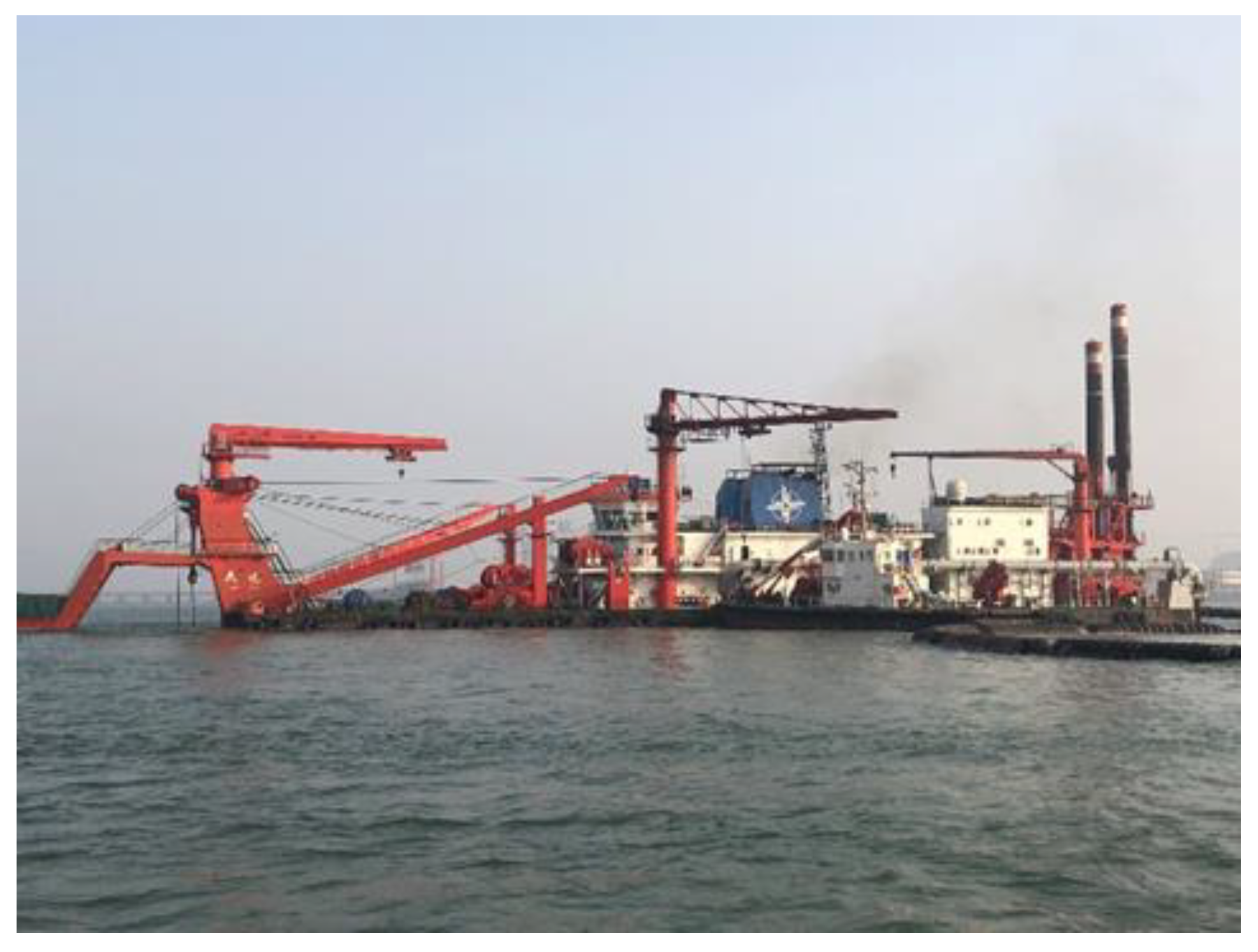
Figure 1.
Field trip map of the dredger.

Figure 2.
Soil test picture. (a) The shear strength curve; and (b) The shear strength curve.

Figure 3.
Particle distribution curve.

Figure 4.
The model test tank. (a) A schematic map of the test tank; and (b) A physical map of the test tank.
Figure 4.
The model test tank. (a) A schematic map of the test tank; and (b) A physical map of the test tank.

Figure 5.
Gravity anchor shear key.

Figure 6.
Model of gravity anchor. (a) Top view; (b) Front view.

Figure 7.
Test pictures.

Figure 8.
Load–displacement curve of the anchor under horizontal loads.

Figure 9.
The 3D finite element model. (a) 3D finite element model of gravity anchor; (b) 3D finite element model of soil.
Figure 9.
The 3D finite element model. (a) 3D finite element model of gravity anchor; (b) 3D finite element model of soil.

Figure 10.
Bearing capacity curves of different elements.

Figure 11.
Numerical simulation result curve.

Figure 12.
Soil deformation diagram of model test and numerical simulation: (a,e) are soil deformation diagrams when the gravity anchor moves 0 mm, (b,f) are soil deformation diagrams when the gravity anchor moves 25 mm, (c,g) are soil deformation diagrams when the gravity anchor moves 50 mm, and (d,h) are soil deformation diagrams when the gravity anchor moves 75 mm.

Figure 13.
Soil flow mechanisms at failure.

Figure 14.
The plastic deformation process of the soil sections at rear of gravity achor.

Figure 15.
Friction angle–reaction force curve.

Figure 16.
Cohesion–reaction force curve.

Figure 17.
The 3D surface plot.

Figure 18.
Anchor bottom area and bearing capacity curve.

Figure 19.
Relationship between mooring point height and carrying capacity. (a) Sensitivity analysis of mooring point height to bearing capacity; (b) Dimensionless relationship between mooring point height and bearing capacity.
Figure 19.
Relationship between mooring point height and carrying capacity. (a) Sensitivity analysis of mooring point height to bearing capacity; (b) Dimensionless relationship between mooring point height and bearing capacity.

Figure 20.
Soil deformation diagram at different mooring heights of gravity anchors.

Figure 21.
Bearing capacity–displacement curve at different stress angles.

Figure 22.
V-H failure envelope of gravity anchor. (a) The V-H envelope of the model test and numerical simulation. (b) Normalized V-H failure envelopes.
Figure 22.
V-H failure envelope of gravity anchor. (a) The V-H envelope of the model test and numerical simulation. (b) Normalized V-H failure envelopes.

Figure 23.
Normalized V-H failure envelope of gravity anchors at different mooring heights.

Figure 24.
Fitted curve expression. (a) D/H = 0 and 0.5. (b) D/H = 0.75. (c) D/H = 1.


Table 1.
Soil particle composition.
| Soil Particle Content (%) | Classification of Soil | ||
|---|---|---|---|
| d > 0.075 mm | 0.005~0.075 mm | d < 0.005 mm | fine grained soil |
| 9.9 | 76.6 | 13.5 | |
Table 2.
Liquid limit and plastic limit test results.
| Liquid Limit (%) | Plastic Limit (%) | Plasticity Index (%) | Classification of Soil |
|---|---|---|---|
| 36.2 | 22.6 | 13.6 | silty clay with low liquid limit |
Table 3.
Soil element number.
| Serial Number | Number of Seeds |
|---|---|
| A | 3 × 3 |
| B | 5 × 5 |
| C | 5 × 10 |
| D | 10 × 10 |
| E | 10 × 15 |
| F | 15 × 15 |
Table 4.
Horizontal bearing capacity with different cross-sectional shapes.
| Section Shape (m2) | Bearing Capacity (N) |
|---|---|
| 1 × 9 | 660,688 |
| 1.5 × 6 | 663,998 |
| 2 × 4.5 | 664,959 |
| 2.5 × 3.6 | 661,374 |
| 3 × 3 | 669,000 |
Disclaimer/Publisher’s Note: The statements, opinions and data contained in all publications are solely those of the individual author(s) and contributor(s) and not of MDPI and/or the editor(s). MDPI and/or the editor(s) disclaim responsibility for any injury to people or property resulting from any ideas, methods, instructions or products referred to in the content. |
© 2023 by the authors. Licensee MDPI, Basel, Switzerland. This article is an open access article distributed under the terms and conditions of the Creative Commons Attribution (CC BY) license (https://creativecommons.org/licenses/by/4.0/).
Share and Cite
MDPI and ACS Style
Yu, J.; Liu, P.; Yu, Y.; Liu, X.; Li, H.; Sun, R.; Zong, X. Research on Bearing Characteristics of Gravity Anchor in Clay. J. Mar. Sci. Eng. 2023, 11, 505. https://doi.org/10.3390/jmse11030505
AMA Style
Yu J, Liu P, Yu Y, Liu X, Li H, Sun R, Zong X. Research on Bearing Characteristics of Gravity Anchor in Clay. Journal of Marine Science and Engineering. 2023; 11(3):505. https://doi.org/10.3390/jmse11030505
Chicago/Turabian StyleYu, Jianxing, Pengfei Liu, Yang Yu, Xin Liu, Haoda Li, Ruoke Sun, and Xuyang Zong. 2023. "Research on Bearing Characteristics of Gravity Anchor in Clay" Journal of Marine Science and Engineering 11, no. 3: 505. https://doi.org/10.3390/jmse11030505
Note that from the first issue of 2016, this journal uses article numbers instead of page numbers. See further details here.