1. Introduction and Background
Route, path, line or way are various terms describing series of interconnected waypoints that a movable entity will traverse or has traversed. For inanimate entities, including land vehicles, aircrafts or ships, routes must be created and adapted to the particulars of the transport mode and voyage objectives. On board ships, the creation of intended routes is still the duty of the navigator(s) and is a part of voyage planning. This is a process, subject to numerous constraints, rules and regulations in which the navigator uses skills, knowledge and experience to create a safe and efficient route for the forthcoming voyage [
1]. During the voyage, the vessel movement, traversed positions and other voyage-related data is saved in predetermined intervals by the onboard equipment, and, if necessary, route retrieval is simple on board. For shipping companies, such route data from ships can be useful for various purposes, including safety of navigation, individual voyages, or even more, fleet efficiency metrics based on length of the route, average speed, traversal time or fuel consumption. Using such data for the wider research community, notably in fleet analysis, is not so common since it is rarely public. However, there are other sources of vessel data, such as data broadcasted from the Automatic Identification System (AIS). AIS data is collected and made available by several public and free sources, including the one used in the conducted research, as will be presented in the following chapter. From the sources, such data can be used for various ship route data purposes.
Route extraction in the context of safe route design, based on AIS data and available categories of ships using Kernel Density Estimation with route boundary extraction and centerline extraction, was considered in [
2]. In [
3], spatial and temporal vessel trajectory clustering in the context of extracting traffic flow information, customary route discovery and anomaly detection was carried out based on AIS data. The trajectories have been investigated in terms of their similarity to Merge Distance. In [
4], computer vision techniques were employed for navigation patterns estimation in the context of traffic statistics and a simplified ship maneuvering model, with traffic group collecting based on geometric similarity using AIS data. In [
5], the Equivalent Passage Plan method, based on the notion that the vessel in navigation follows a prepared voyage plan, was used as a framework for trajectory simplification and event identification in the context of ship behavior extraction. Further, the Hausdorff distance was used to measure similarity between the simplified and original AIS trajectories. Hausdorff and other similarity methods can be broadly grouped into warping-based methods and shape-based methods. The warping methods include Dynamic Time Warping (DTW), the Longest Common Subsequence (LCSS), and the Edit Distance on Real sequence (EDR). Shape-based methods include the Hausdorff distance, One Way Distance (OWD), and the Fréchet distance [
6]. Similarity measures can be used in spatial, temporal and spatiotemporal contexts. For spatial contexts, the measures can be compared topologically and quantitatively, in terms of global and local path similarity, travelled distance, range and shape [
7]. After assessing the available various route research interests and similarity methods, it is important to present a brief overview of AIS, the data source on which route analysis and similarity methods are employed in the maritime context.
AIS is a digital short-range automatic data exchange system operating at a very high frequency (VHF) band. Although it was devised as a terrestrial system, AIS signals can be received by satellites as well. Its use is mandatory for all ships under the requirements of the International Convention for the Safety of Life at Sea (SOLAS), determined by the International Maritime Organization (IMO). Although used primary in maritime contexts such as ship identification, collision avoidance or traffic monitoring [
8], the available AIS data is a valuable source for various research interests [
9]. AIS data is static (e.g., ship identification, basic dimensions, type), dynamic (e.g., position, speed over ground, heading), voyage-related (e.g., navigation status, draft, cargo type) or in form of short safety-related messages. SOLAS-regulated Class A ships send their dynamic data messages in intervals dependent on ship speed and course change. Intervals start from between 2 and 12 s, when the ship is underway, and are 3 min when it is anchored or moored [
10]. Further, AIS provides several identifiers for special crafts (e.g., pilot vessels and tugs) and ships such as high-speed crafts (HSC), cargo ships, tankers, passenger ships and ships from the other ships category [
11]. Although beneficial for broad ship-type categories, the shortcoming of AIS categorization appears when the research focus is on different categories of ships, such as general cargo ships and container ships. They are both cargo ships; however, they lack separate AIS categories. This makes it more difficult, for example, for evaluation comparing single or multiple fleets, or evaluation of previously stated different cargo ship classes. This was confirmed in the research literature, since the available articles on the subject are rather limited. With the observed gap, we decided to evaluate if the available approaches using AIS default categories in route analysis could be further extended for single or multiple ship fleet analysis.
When assessing ship route research objectives using AIS data [
12] and including similarity measures, frequently applied approaches consider general AIS ship categories or created subcategories for route and traffic analysis [
13]. In [
14], authors examined and delineated maritime routes between ports along the Atlantic coast of the USA using AIS data from 2010 to 2012. Commercial tracks were generated for commercial vessels, with a focus on cargo vessels. The routes were delineated with a 95% boundary of all traffic transiting each route. In [
15], authors analyzed ship traffic demand and the spatial–temporal dynamics in Singapore port waters using AIS data. They found that origin-to-destination pairs and navigation routes in the area were stable and found several hotspots with high speeds. In [
16], authors evaluated trajectory clustering for marine traffic pattern recognition around the Chinese Zhoushan Islands from January to February 2015. A Density-Based Spatial Clustering of Applications with Noise (DBSCAN) algorithm with improved parameters was proposed. In [
17], authors devised a method to transform the ship trajectory into a ship trip semantic object (STSO) with semantic information. Authors used graph theory, and integrated STSO into the nodes and edges of a directed maritime traffic graph for route extraction. The AIS data was data collected from 1 January to 31 December 2017 from crude oil tankers in the Asia-Pacific and Indian Ocean regions. In [
18], a ship AIS trajectory clustering method based on the Hausdorff similarity distance and a Hierarchical DBSCAN (HDBSCAN) was used. AIS data on the estuary waters of the Yangtze River in China was used and compared with k-means, spectral clustering and DBSCAN.
As we have presented, there are various route research approaches and interests using AIS data for route and trajectory research. Similarity measurement is used in numerous contexts of AIS data, route and trajectory analysis. Although diverse types of ships were covered in the presented papers, route comparison between other groups of ships besides general AIS ship types is not very well researched. With such observations, we focused our selection on the cargo ship subcategory, which could be suitable for fleet selection and analysis.
Accounting for 13.34% in 2022 of total world fleet by deadweight, container ships are the third largest principal vessel type, behind bulk carriers and oil tankers [
19]. Further, the assessment of container ship routes and fleets has several possible advantages over the assessment of other principal vessel types. Vessels are employed in liner services, with companies usually providing public data on their services and vessels. In regular operation, vessels call on the same service ports according to their schedules, thus enabling route comparison in both spatial and temporal domains. Moreover, 4 large carriers (MSC, APM-Maersk, CMA CGM and the COSCO group), accounting for more than 50% of capacity, dominate the market [
19], facilitating the collection of significant route data, which can be interpreted for individual fleets or used to make inferences about total container fleet insights.
A broad overview of container ship fleet research topics includes various levels of planning and decision-making, liner shipping networks, scheduling, fleet compositions and deployment, air emissions, optimization and routing, resulting in a considerable body of literature [
20,
21,
22]. Further, ships and fleet route elements are commonly evaluated in terms of speed and speed optimization [
23,
24,
25] or trajectory and speed distribution [
26]. Speed accuracy is evaluated as well, using the collected speed through water (STW) data of 190 container vessels from Maersk [
27]. However, literature on container ship fleet route analysis is scarce. An operational analysis of container ships using AIS and environmental data was carried out [
28] based on Hortonworks’ big data framework. Trajectories and speeds from several voyages were compared to evaluate voyage energy efficiency for a single 10,000 TEU ship and four 13,000 TEU sisterships. A speed pattern analysis was carried out for 8600, 13,000 and 18,000 TEU ships from several companies, whereas route similarity was not considered. Container ships and fleets were analyzed, using AIS data collected in a database from along the Portuguese coast for top container carriers, services, and vessels [
29]. Routes were characterized for individual ships, indicating the sequence of visited ports, respective travel times, the total number of trips and carrying capacity. However, spatial distributions of routes and their similarities were not investigated. In [
30], vessel speed, course and path analysis in the Botlek area of the port of Rotterdam was assessed for five container ship categories along with other vessel types. This research was further extended in [
31], where a comparison study on AIS data with a characterization of ship traffic behavior was carried out. The data was evaluated for traffic modelling and simulation in restricted waterways. Research areas were a narrow waterway in the port of Rotterdam and the Yangtze wide waterway area near the Su-Tong Bridge. Spatial distributions perpendicular to the water flow and to the channel, sailing speeds, average speeds and course distributions were analyzed. Again, route similarities were not assessed in either of the articles. As can be observed, route similarity measures are usually not considered in either general container or individual fleet analysis.
With that notion in mind, we selected container ships as a subcategory of interest extracted from the total cargo ships category and examined it in terms of route characteristics and similarity.
A fleet of container ships from a single shipping company employed in regular service calling on the ports of Savannah and Charleston on the east coast of the USA was chosen. The selection was chosen due to the similar constrained conditions of the selected ports and possible routes and expected navigational decisions made when planning and executing the voyage.
The remainder of this paper is structured as follows. In
Section 2, we present the methods used in the research; we introduce the research area and describe the pre-processing of AIS data, route creation and similarity measurement. In
Section 3, we present the research results and findings.
Section 4 is the discussion, and we present the conclusions with future research suggestions in
Section 5.
2. Methods
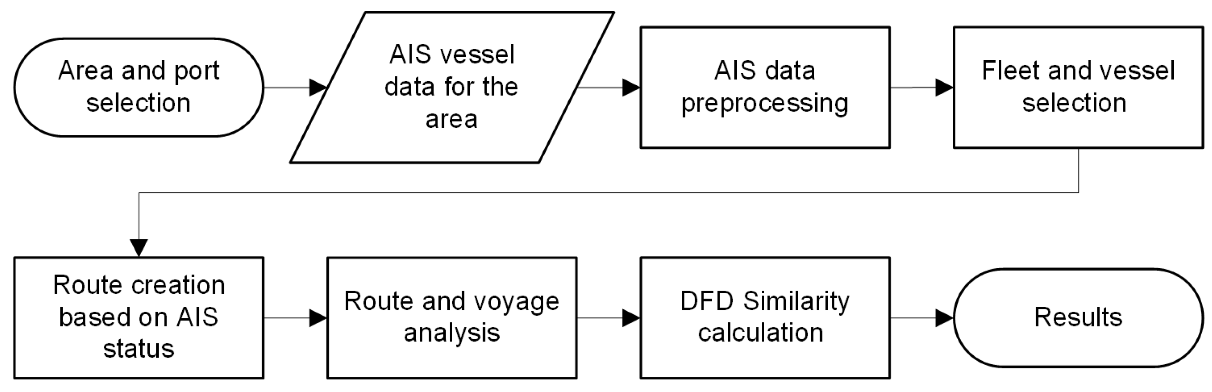
To evaluate the differences between the ship routes, several conditions were considered. The ports and area of interest should be located in relationship to one to another to provide modest route choice variability, within a somewhat constrained area. Further, the ports should be called on regularly by major companies of interest to facilitate fleet creation from available collected and processed data. From several candidate pairs, the ports of Savannah and Charleston were chosen. Their respective details and further methodology will be described in the following paragraphs along with a prior general overview, presented in
Figure 1.
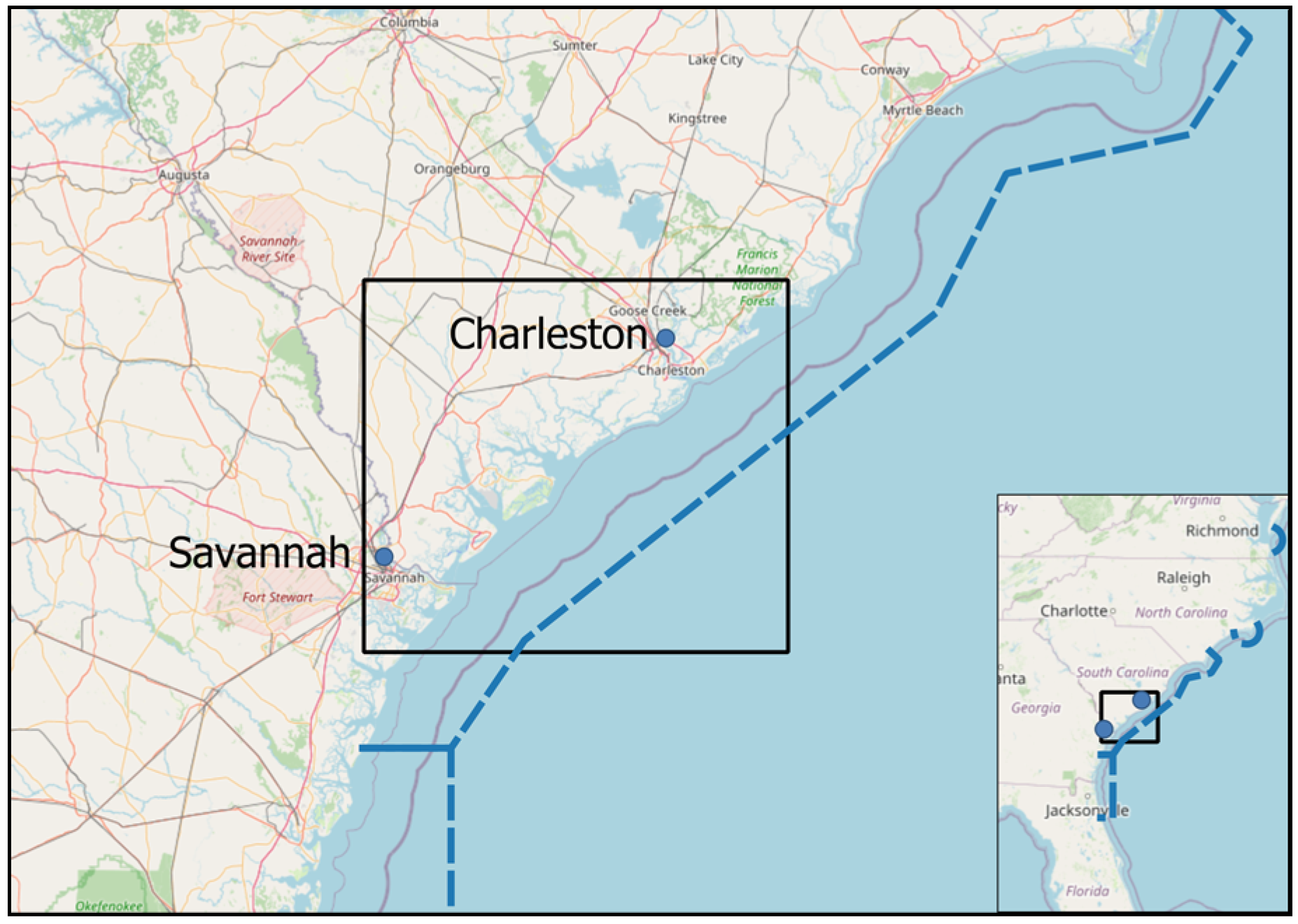
The data collected and used is publicly available AIS data from the NOAA AccessAIS portal [
32]. The observed period starts on 1 January 2019 and ends on 30 June 2019. The area of interest (AOI) is bounded by 31.791° N, 81.224° W, 33.102° N and 79.453° W, as presented in
Figure 2. This is the coastal area between two major USA East Coast ports of interest, Savannah and Charleston. The respective ports, besides handling several other types of cargo, are major hubs for containerized cargo.
During the fiscal year 2019 (ending 30 June 2019), 1848 ships called on the Savannah Garden City Terminal with 4.48 million twenty-foot equivalent units (TEUs) handled. The projected increase in cargo volume for the year 2030 was 48% [
33]. In the port of Charleston, the Wando Welch and North Charleston terminals handled 2.93 million TEUs. At all the Charleston cargo terminals, a total of 1696 vessels called in the 2019 fiscal year [
34]. Further, vessels from several major container carriers and alliances call on the ports regularly as a part of their services.
According to [
35], the distance from Savannah to Charleston is 104 nautical miles (NM). The calculated distance is measured along navigable tracks as the shortest route for safe navigation between the two ports. As we present in the results section, the actual distances for the selected ships are greater due to several reasons, including the size of the ships and the characteristics of the navigational area.
Besides the importance of the respective ports and the significant vessel traffic they generate, we must emphasize that the coastal area is part of the North Atlantic right whale Seasonal Management Areas (SMA). All vessels with length overall (LOA) of 65 feet (19.81 m) or greater and subject to the jurisdiction of the United States are restricted to speeds of 10 knots or fewer in a continuous 20 NM Seasonal Management Area between 1 November and 30 April annually [
36]. The areas were established to prevent collisions of vessels with endangered right whales.
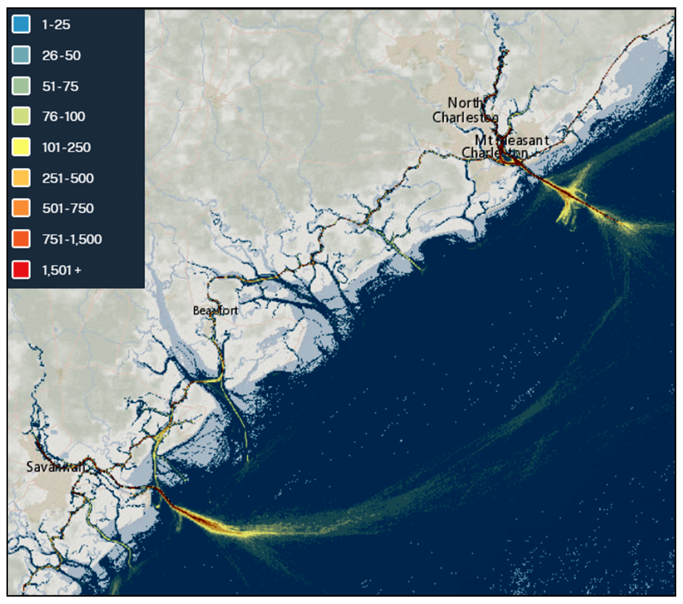
To identify the patterns of interest for route creation, available vessel density data for the AOI was investigated. The data is available as a publicly available annual AIS vessel count dataset for the USA and international waters. The annual data is summarized using 100 m by 100 m geographical grid cells with single transits counted each time a vessel track passes through, starts or stops within the grid cell [
37]. A simplified geographical area subset transit density graph can be obtained through the AccessAIS portal as well, as presented in
Figure 3.
We conducted data preparation and preprocessing using the Python programming language; version 3.10.4, the Pandas data analysis library [
38], version 1.4.2 [
39]; the Shapely package for computational geometry [
40] and the NumPy array programming library [
41], version 1.21.6. To create routes, we used the MovingPandas library [
42], version 0.9.rc3 [
43]. The library is based on Pandas, GeoPandas, an extension to Pandas enabling spatial operations on geometric types [
44], and HoloViz high-level visualization tools [
45]. A trajectory in MovingPandas is defined as a time-ordered series of geometries and can be point or line based.
From the whole dataset, we selected cargo ships by the AIS ship code (70 to 79) used for cargo ships [
46]. The cargo ship subset included 724 unique entries. To create a container ship fleet subset, we collected publicly available fleet data about ships and selected ships by their names and identities. The container fleet from the selected company included 22 unique ships with 107,977 cumulative AIS observations and data entries. From the ship identities, a trajectory collection was created for all 22 unique ships. A single trajectory entry in the collection accounts for all ship observations throughout the six-month period. There are several approaches available for the creation and separation of trajectory entries into individual voyages and routes with available MovingPandas functions. They are based on regular time intervals, speed, stopping and observation gaps. Since the AIS data includes the navigational status of the ship—which is 0 for the ship when underway using its engine—the individual voyages were split at entries when the ship status changed from underway to moored or anchored. We must emphasize that the change of a ship’s navigational status in AIS must be changed manually on board. If not done in a timely manner, this could lead to false interpretations of a ship’s stopping or movement and result in erroneous statuses. However, in the observed dataset, this was not the case, and there were no significant discrepancies between ship status and individual voyage delineation. Further, compared with other available MovingPandas splitting approaches, the preselection by status yielded better results in the splitting up of individual voyages (or trajectories, as implemented in MovingPandas). To reduce the number of unnecessary voyages and split the voyages accordingly, the observational gap value between observations was set to 30 min and the minimum length of the trajectory was set to 200 km (to approximate the distance between ports). With these constraints, the subset was reduced to 13 ships with 23 individual voyages. We created the final subset by choosing the general direction (between 050° and 060°) from individual trajectory start and end points from Savannah to Charleston. The final subset therefore includes 12 voyages (trajectories) from 8 ships. Basic ship particulars are presented in
Table 1. The ships in the subset are sorted by overall length and principal dimensions. The abbreviations and acronyms are described as follows: Length Over All (LOA), Breadth extreme (B
ext), Draught maximum (D
max), Draught per voyage in meters (D
voy) and deadweight (DWT) in metric tons. IDs are designated as letters with added numbers for individual voyages.
After the creation of individual voyages, we evaluated the route lengths, voyage durations, average speed in knots (kt) and similarity between individual routes. Among numerous available similarity measures, Fréchet distance (FD) or, formally,
is often used [
47]. It is described intuitively as a leash length between a person and a dog walking on their respective curves. They can have independent velocities, stop, and start; however, they cannot go backwards. Therefore,
can be described as the shortest possible leash length for the completion of the walk. In a formal way, we can then define a curve as continuous mapping
where
and
are in metric space
. Two continuous curves,
and g
with their
can be defined as [
47]
where continuous nondecreasing functions
. The continuous curves can be further approximated as discrete polygonal curves. Therefore, an approximative discrete Fréchet distance (DFD) or coupling distance
can be calculated. The polygonal curves can then be defined as
with corresponding sequences
and
with coupling
L, which is a sequence of distinct pairs of points of curves
P and
Q, respecting the point order (
,
), (
,
), …, (
,
). The first and last point pairs must be ordered as
. For all subsequent points
, we have
. The maximum distance
between the point pairs for a given coupling
L is therefore the coupling distance. We can then define the discrete Fréchet distance as the minimum distance between all possible couplings between
P and
Q [
47].
Therefore, using the previous person and dog or frog hopping analogy—since we consider discrete movement—we can describe the pair matching and discrete distance calculation. The person and dog can stay on their current vertices, while the other advances or they both advance to the next vertex on their respective paths. The DFD is then the smallest distance for the whole sequence of jumps to the last vertices.
The advantage of DFD over continuous FD is that it has a reduced computational cost while being a good approximation of the continuous solution. Further, provision of an upper bound on the continuous FD is provided, and the deviation is not greater than the longest edge of the trajectory [
48]. Finally, the chosen DFD implementation [
49] used in our research is based on the algorithm from [
47].
Compared to other similarity measures such as Hausdorff distance, FD (and variants) is more useful for comparing curves, since it considers location and ordering of points of the curve [
50]. The chosen DFD implementation is available in the Python similarity measures library, which includes Dynamic DTW, Partial Curve Mapping (PCM), Curve Length (CL) and other similarity measures [
51].
The basic implementation of the similarity measures library considers the calculation of similarity between two curves only, so we had to extend the approach as follows. To calculate DFD values, we created 2D arrays of latitude and longitude coordinate pairs from individual ship position entries. The position coordinates, which were defined using the angular World Geodetic System (WGS84), were transformed into local planar-projected Universal Transverse Mercator (UTM) zone 17N system coordinates to improve the accuracy of the implemented DFD approach. Then, a square mesh grid consisting of individual route arrays with coordinate pairs was created. A vectorized DFD method was then applied to obtain the similarity results, which are presented in the results section.
3. Results
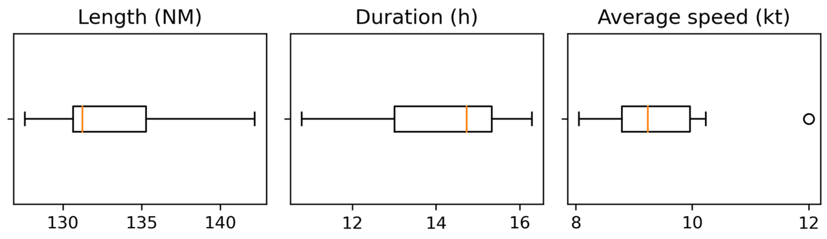
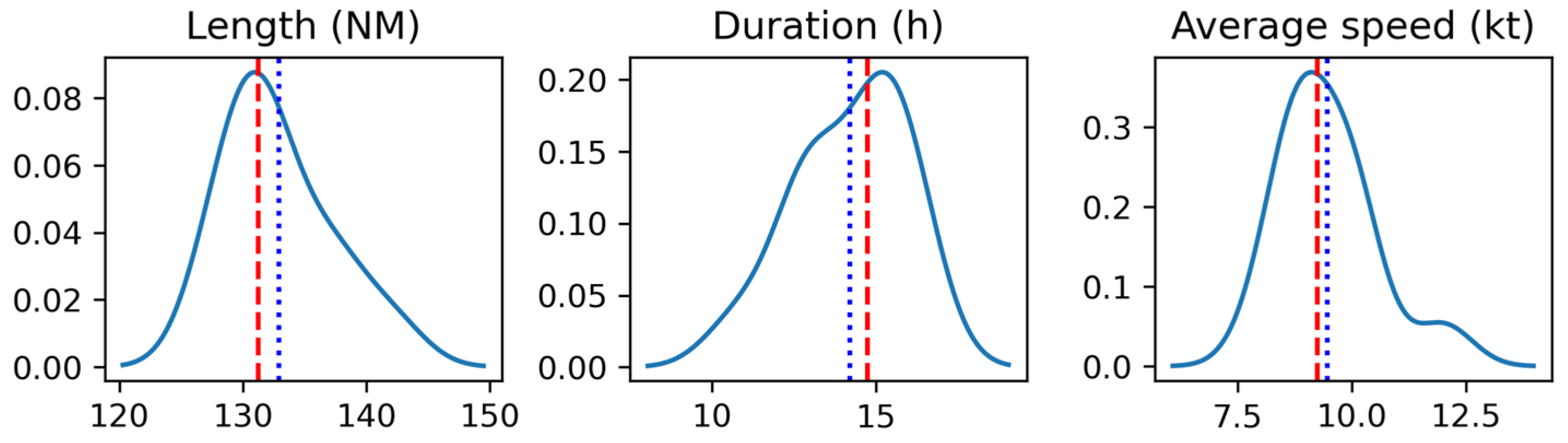
Basic features are summarized in three voyage values: length in nautical miles (NM), duration in hours (h) and average speed in knots (kt). These values, in the form of statistical summary, are presented in
Table 2, along with boxplots in
Figure 4. The values represent length in nautical miles (NM), voyage duration in hours (h) and average ship speeds in knots (kt).
As is observable, the mean value of voyage length is 132.9 NM with a standard deviation of 4.4 NM, whereas the difference from the shortest to the longest voyage is 14.6 NM. The mean and median length values are close; however, the distribution is moderately positively skewed with a value of 0.77. The skewness value is calculated as an adjusted Fisher–Pearson coefficient of skewness with classification as in [
52]. This classification is as follows: normal (−0.5 to +0.5), moderately skewed (−1.0 to −0.5 and +0.5 to +1.0) or highly skewed (<−1.0 or >+1.0).
The next value is the distribution for the voyage duration in hours. The difference is 5.2 h between minimum and maximum value, whereas the mean value is 14.2 h. The distribution is moderately negatively skewed (−0.62) as is observable in
Figure 4 and
Figure 5, in which other distribution characteristics are visible as well.
The last distribution is for the average speed with a difference between minimum and maximum of 3.9 kt. Further, the maximum value can be considered an outlier (outside the interquartile range multiplied by 1.5), which is observable in the boxplot in
Figure 4. However, since this not an erroneous value and the sample size is small, we did not remove it from analysis. Further, the distribution is highly positively skewed (1.23), which can be seen in the respective plot in the
Figure 5.
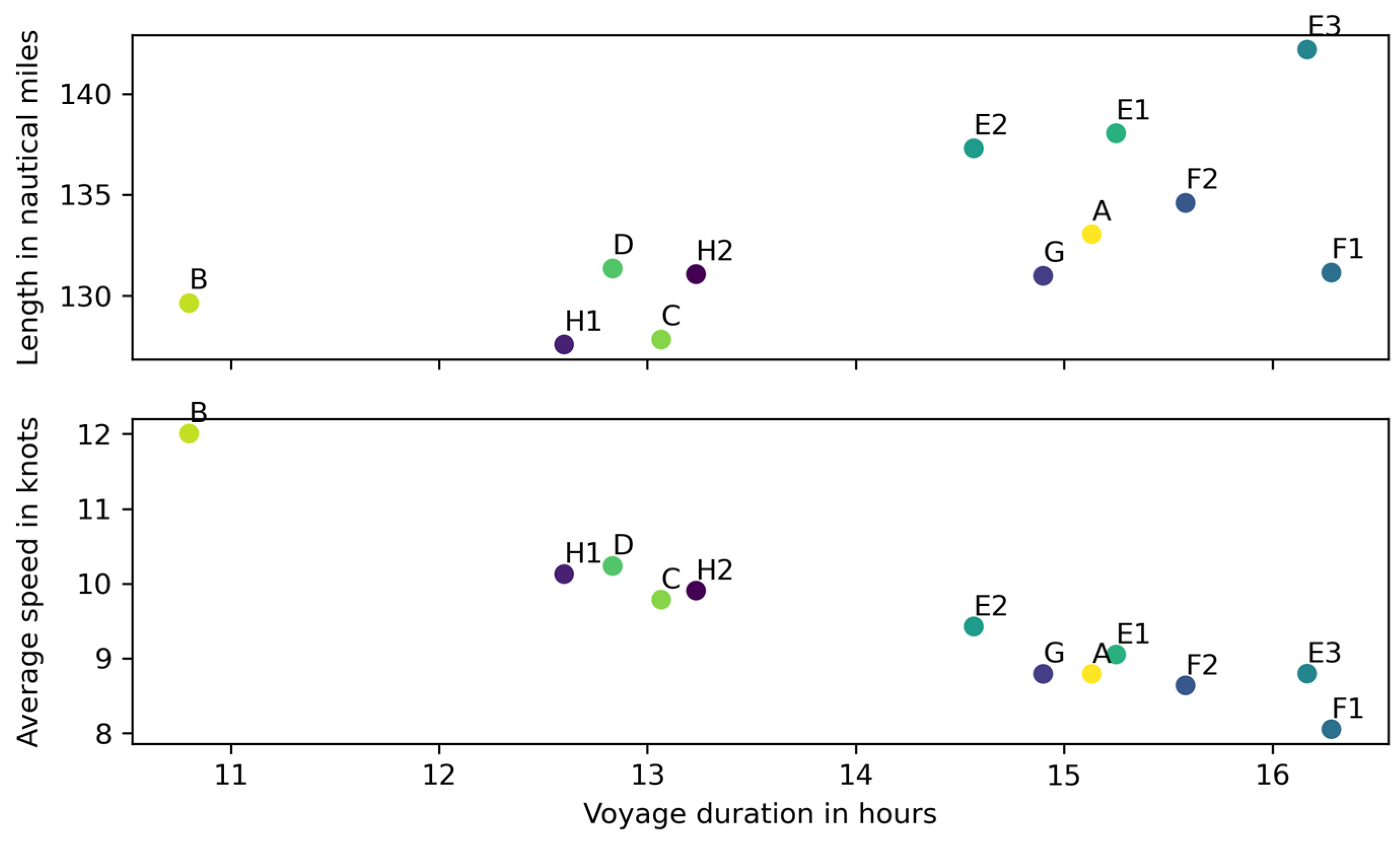
Since the number of voyages is small—compared to overall voyages conducted over several years, or total numbers that include other ships and fleets on this service—we did not make further inferences by using methods to test distributions, either for normality or for underlaying distribution determination. This will be addressed further in future research. The actual distribution of individual voyage lengths and speeds can be observed in scatterplots in
Figure 6.
There are three clusters observable. First, a single entry for ship B, with the shortest voyage length and highest average speed. Second, centered on about 13 h of voyage length, including ships C and D with 2 individual voyages of ship H (H1, H2). The third cluster spreads out between 14 h and 16 h of voyage duration and includes the remaining ships: A, E, F and G.
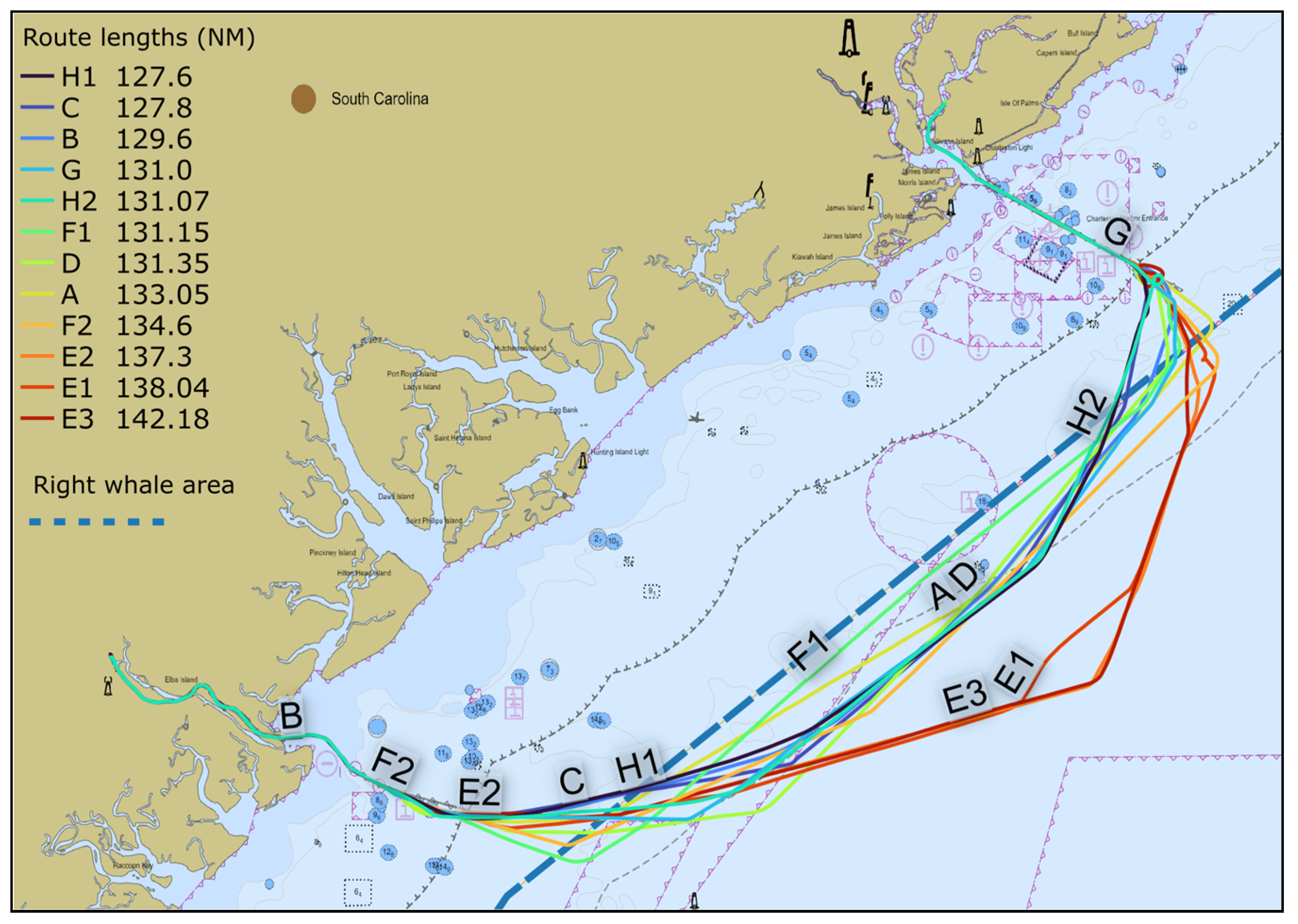
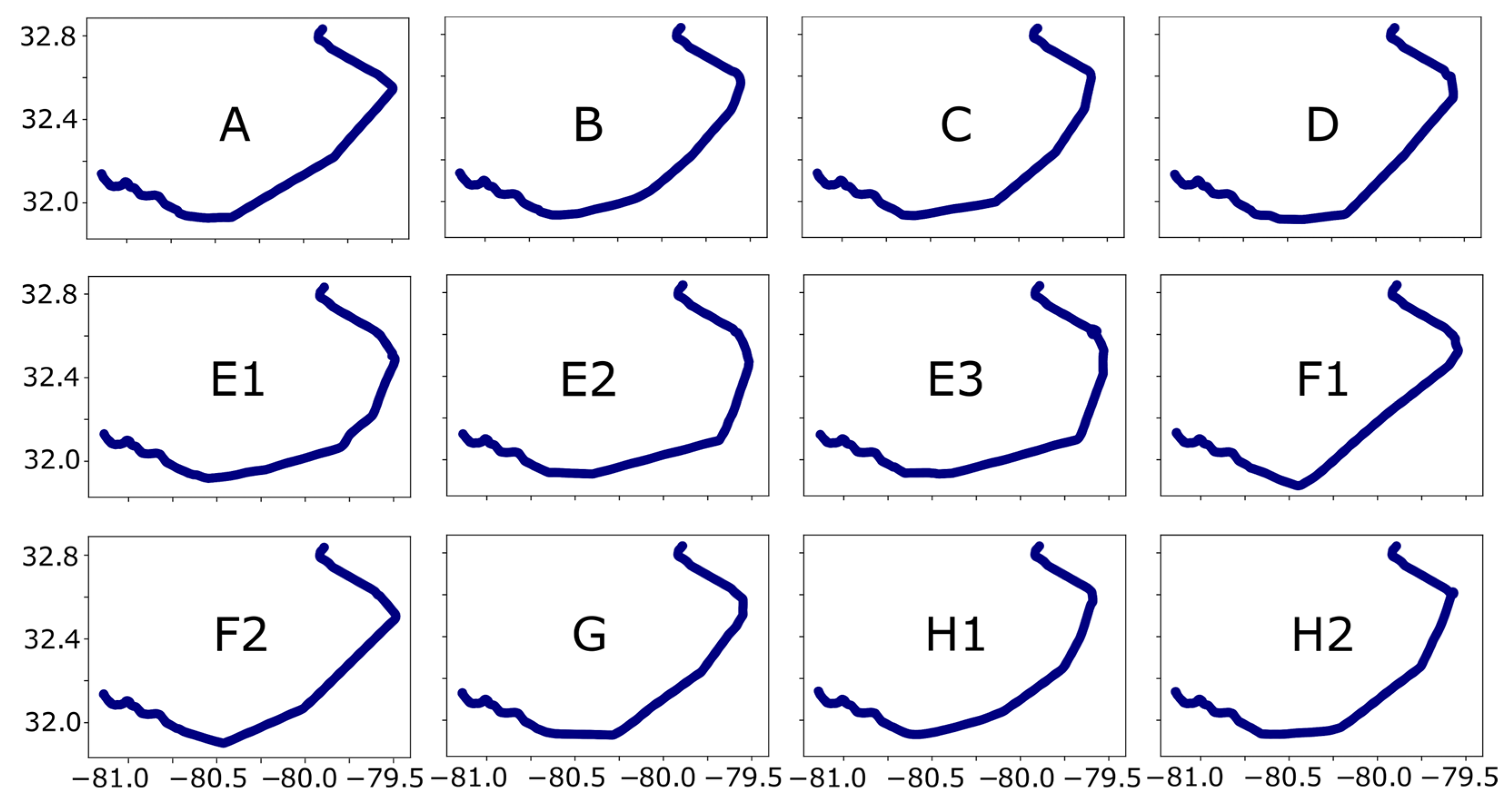
The characteristics of individual ship routes and their spatial distribution can be observed in
Figure 7. Seen beside the visible individual ship routes, the dashed line represents the Seasonal Management Area boundary, and we can see that the ships were sailing outside the area after passing the port approach areas for Savannah and Charleston.
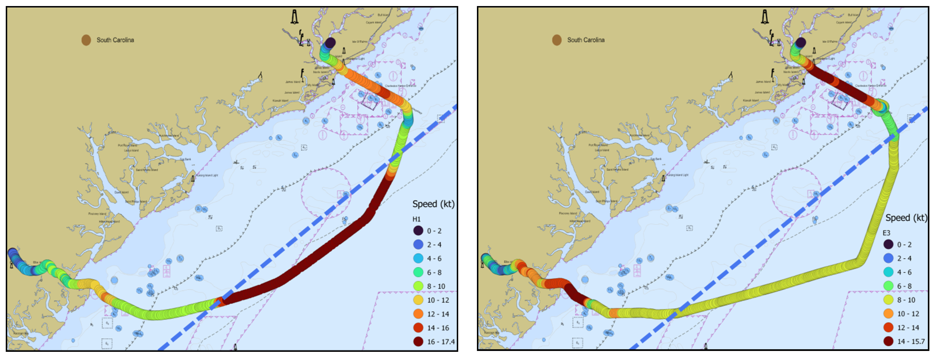
Further, we examined the trajectory profiles for the longest and shortest route (H1 and E3) presented in
Figure 8. The route length for ship H in voyage H1 (27 January 2019) was 127.6 NM with a passage time of 12.6 h, which was accounted for by an average speed of 10.1 kt. On the other hand, the voyage with the highest average speed of 12 kt, for ship B, was completed in 10.8 h with a total length of 129.6 NM. Ship E, in voyage E3 (14–15 April 2019), completed the respective voyage in 16.2 h with a total length of 142.2 NM with average speed of 8.8 kt. The voyage with the lowest average speed of 8 kt was conducted by ship F in voyage F1, with a total route length of 131.1 NM. The following route comparison could be expressed in terms of highest and lowest speeds, although we present the cases by route lengths only.
Besides the route selection and length, there are differences in speed profiles as well. Ship H1 had a significantly higher speed in the central part of the route between the Savannah and Charleston approaches. For ship H, the speed was over 16 kt to a maximum of 17.4 kt, as was reported in SOG values in AIS data. Ships sailed with required speeds in the SMA and stayed outside the coastal areas in which there are obstructions and fishing facilities which could be dangerous to navigation, as is visible in
Figure 9 (left). Further, we can observe differences in the Charleston approach and pilot boarding area (in vicinity of Charleston Entrance; buoys not visible on presented figures). Some of the ships proceeded directly, while two ships (H2, E3) made turns while presumably picking up the pilot.
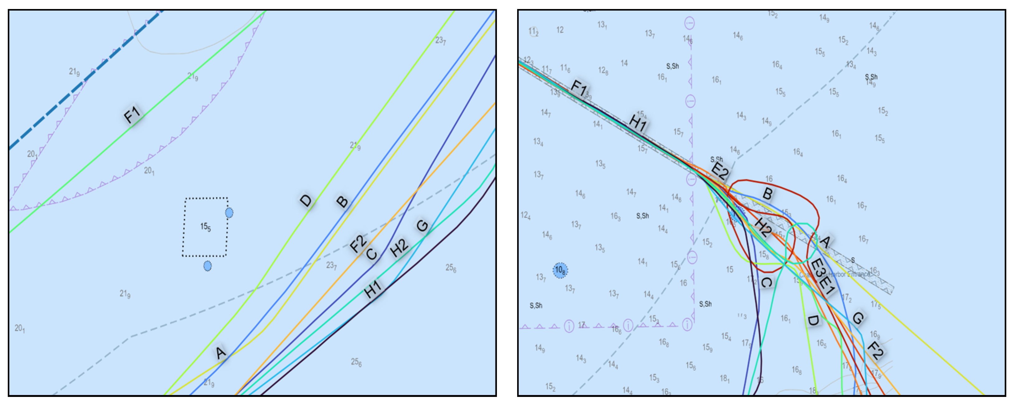
Finally, we evaluated the routes in terms of similarity. The individual routes are presented in
Figure 10 as a reference. We can observe that route parts in constrained areas of navigation such as port approaches or river passages were similar. The differences arose with choices about whether to pass northwards or southwards to avoid several obstructions, which can be observed in previous figures.
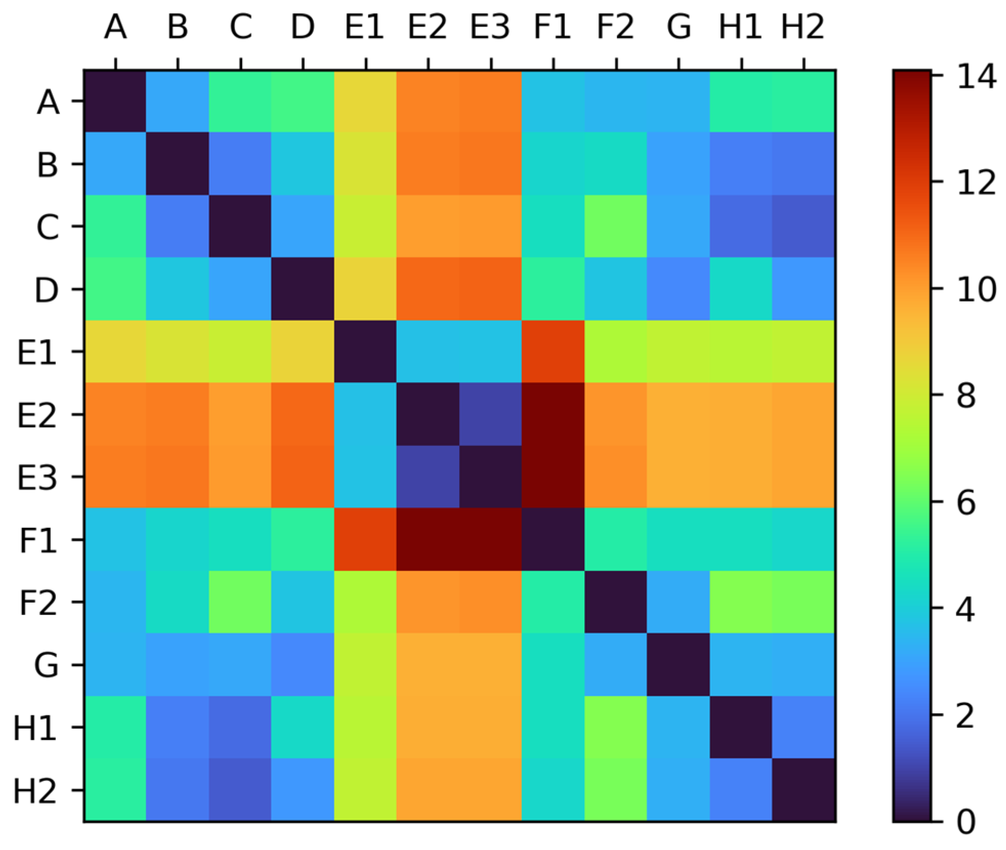
The calculated DFD similarity values are presented in
Figure 11 as a heatmap. The lower values and darker color intensity indicate higher similarity. We can observe several routes with higher similarity. The calculated values are the distances in nautical miles.
There were similarities among the different voyages from the same ships (E1–E2–E3, F1–F2 and H1–H2). Further, the highest route similarity between different ships was for ship C and ship H, whereas the lowest similarity was between routes from ships E and F. The calculated DFD similarity value complements the interpretation of similarities of visual or geographical routes and the statistical analysis of voyage data.
4. Discussion
The aim of our research was to analyze general route characteristics and evaluate similarity for a container ship fleet of a single company. As the preliminary research literature showed, route and similarity analysis considering fleets is not common. Reasons might include the perception of the availability of data and tools for such analyses. Formatted public AIS data records are available from NOAA, other national providers, and at times as sample or test datasets from private providers. The other challenge is collecting the ship data on which fleet assessment is based. This includes information on ship fleets and categories other than general AIS ship type categories. Nevertheless, the data can be collected from shipping companies and other reliable online sources such as shipping vessel registers and official international or national vessel data providers. However, this is a time-consuming process. Although there are many private providers which can provide aggregated ship data on companies and fleets with detailed ship types, the financial aspect of acquiring data might be worth consideration or even be a barrier for those interested.
For route characterization, we selected the two ports because of their proximity and constraints in the number of possible routes. As expected, the sailed routes taken by ships of different sizes were mostly similar, notably for the same ships. The route differences arose after the port approach areas were passed and the right whale protection area, which all the ships sailed outside, was exited. This was presumably due to the right whale avoidance and speed constraints required during the period of the SMA (from 1 November to 30 April 2019). Further, even after the end of the SMA period, the vessels sailed outside the area. It must be seen in future research if this occurs during the rest of the year. Further, as we presented regarding ships’ particulars, the maximum and reported voyage drafts were large, ranging from 14.5 to 15.5 m, with only one vessel (C) reporting a lower voyage draft (12 m) than the maximum (15 m). Therefore, to keep a safe depth below keel, referred to as Under Keel Clearance (UKC), ships must stay in the deeper waters with depths of 20 m or more, which are outside the SMA area. In the shallower area near the coast, there are obstructions and fishing facilities as well, so even in that context it is safer to stay in the deep-water area.
Route characteristics do not differentiate substantially. There are differences in length which we can attribute to collision avoidance, besides route choice by the navigator. However, to confirm that decisively, we should evaluate the surrounding traffic as well. Looking in terms of route length, voyage duration and speed, most of the observations are not very dispersed either from the mean or median values. The distribution shapes reveal moderate to high skewness; however, the number of voyages and routes is too low to give decisive conclusions, and further tests should be conducted regarding the type and shape of the underlaying distribution. Further, assessment of the individual voyages reveals there is some clustering of individual routes, considering both voyage length and duration. The shortest voyage duration was 10.8 h, compared to 16.3 h for the longest voyage. The mean and median values of the average speed are 9.5 kt and 9.2 kt, with only one vessel sailing with an average speed of 12 kt. This along with trajectory analysis reveals differences in the speed profiles of the vessels, at least during parts of their routes. The fastest-average-speed vessel had much more variable speed (H1) throughout the voyage than the vessel with the lowest average speed (E3). To better understand behavior in parts of the voyage, additional trajectory analysis is required, and identification of regularities in behavior, if they exist.
The similarity measurement revealed that the same vessels take more similar routes in different voyages compared to the rest of the vessels. This is observable both in visual shape evaluation (vessels E, F and H), which was applicable in our study, and with DFD similarity measurement. This similarity should be assessed against a baseline route which either is derived as a generalization from numerous routes or is a route devised by a navigator in accordance with established voyage-planning procedures. The DFD pairwise similarity measurement, visual inspection for a small number of routes and methodology, is applicable. However, there is an issue of computational cost for DFD calculation of substantial numbers of routes. We did not generalize the routes due to the small number (several hundred for each route) of AIS data entries—points regularized at approximately one-minute intervals by default in NOAA AIS datasets. The number of entries can be reduced even more with route generalization and the extraction of important route points (e.g., when the vessel alters the course) and omission of the rest. This would reduce computation time when dealing either with substantial numbers of points per voyage or substantial numbers of voyages. Further, other similarity measures should be used as well for comparison. To evaluate usability, in forthcoming research we will assess DFD against other similarities in other shipping areas and with other ships and fleets.
Our methodology builds on established tools and practices for data assessment and similarity measurement, along with our own approach to similarity comparison between the individual ships or entire fleets. Since we conducted the analysis with open-source software based on the Python programming language, other interested researchers can apply the described methodology. Finally, the usage of discrete Fréchet distance to measure similarity of the routes is a valuable addition to route knowledge interpretation. It formalizes the route similarity in a single value; likewise with the route length, which is one of the values with which we compare the routes. The use of DFD values can be applicable in a variety of contexts, such as limiting values for the route selection from a trajectory collection. It can be used for similarity values when comparing planned routes on board ships, besides visual inspection and leg by leg comparison. Further, it can be used as an indication of possible route deviations in the context of the safety of navigation. This can be extended to creating profiles of various ship categories based on different criteria such as fleet, class and sizes.
Finally, we must state that we expected high similarity due the area characteristics, fleet selection, route possibilities and expected ship behavior. Further, this methodology opens new possibilities of knowledge discovery between diverse groups of ships, such as fleets, which are not observable when considering general ship groups.
5. Conclusions
Ship route analysis often considers general route and knowledge extraction in spatial and temporal dimensions. With AIS historical data availability, such a process is simpler than it used to be. However, since the available AIS ship types are limited, analysis for various ship groups has its challenges. With our methodology, we examined route characteristics both in statistical terms and using discrete Fréchet distance for the measurement of similarity for a single container ship fleet. This opens the possibility for the comparison of route creation and execution, not only between similar types of ships, but with fleets as well.
The investigated routes shared similarities in length, duration and average speed; however, there are differences between route legs, where we observed differences in speed profiles. Due to ship size, draft, speed limitations and the avoidance of obstacles in the coastal right whale protection area, ships stayed farther from the coast and outside of the area.
In terms of visual and numerical similarity, we observed that the same ships in different voyages tended to have similar routes. The route similarity between other vessels was also observable, as we expected, due to the relative proximity of, and limited number of potential routes between, the ports. The DFD similarity measure adds value to route interpretation with common values such as route length and duration. We extended the route and similarity analysis from general research on ship categories to fleets, which is not as common. Further, we extended the methods from known software libraries, which were not designed specifically for AIS data analysis, and therefore do not have all the specific functions that could apply when dealing with AIS data. The proposed methodology is based on open-source libraries and data, and can be adapted for further applications. It is our belief that our methodology can improve the reproducibility of similar research approaches and future frameworks.
For future research, we will evaluate longer time periods and datasets to obtain more routes for the comparison of ships in a single fleet and between fleets. We will evaluate methodologies for more distant ports and use other similarity measures. Trajectory analysis will be considered as well, to evaluate the speeds between different route legs.


