Article

Fatigue Strength of AH36 Thermal Cut Steel Edges at Sub-Zero Temperatures

Institute for Ship Structural Design and Analysis, Hamburg University of Technology, 21073 Hamburg, Germany
*
Authors to whom correspondence should be addressed.
J. Mar. Sci. Eng. 2023, 11(2), 346; https://doi.org/10.3390/jmse11020346
Submission received: 25 November 2022 / Revised: 13 January 2023 / Accepted: 31 January 2023 / Published: 4 February 2023
(This article belongs to the Special Issue Fatigue and Fracture Mechanics of Marine Structures)

Abstract

:
Cruise ships or yachts that operate in areas with seasonal freezing temperatures have large openings in the outer shell. Those are thermal cut edges, and they are exposed to very low temperatures. From fatigue crack growth testing of base materials, it is known that low temperatures can accelerate the crack growth, which may reduce the fatigue life of a structure. However, the current guidelines and rules of classification societies do not provide design curves for the fatigue assessment of thermal cut steel edges at sub-zero temperatures. Therefore, fatigue tests of thermal cut edges are conducted at −20 °C and −50 °C as well as at room temperatures for reference. The specimens are plasma-cut and tested in a temperature chamber under uniaxial loading with a resonant testing machine. The test results are statistically evaluated using linear regression and the maximum likelihood method. The results show that the fatigue strength at sub-zero temperatures is significantly higher compared to room temperature. The test results of this study indicate that sub-zero temperatures down to −50 °C do not seem to cause a reduced fatigue life of thermal cut steel edges.

1. Introduction

Sub-zero temperatures influence the fatigue strength of ship structures. Apart from the root and toe failure of welds, free thermally cut steel edges are also critical details in the ship structure for crack initiation under cyclic loading. Especially the ship hull of modern cruise ships and large yachts, which hold a significant number of openings for windows and balcony doors (Figure 1). When these kinds of ships operate in polar and subpolar conditions, those cut outs may be exposed to very low temperatures, which may lead to a change in their fatigue behavior. Low temperatures refer to a combination of air temperature and the wind-chill effect (e.g., the temperature–humidity–wind index, THW index), which may lower the temperature by 10 °C or even 20 °C.
The fatigue performance of free plate edges [1,2,3] is researched for normal temperatures and also the effect of high temperatures is considered in the standards for the fatigue assessment of steel structures. Accordingly, current standards such as the recommendations of the International Institute of Welding (IIW) [4] provide a factor for fatigue assessment at high temperatures, which depends on the modulus of elasticity; however, studies on the impact of sub-zero temperatures are scarce.
Experiments of crack growth in the base material revealed that the fatigue of ferritic structural steels with a body-centered cubic crystal structure undergoes a ductile to brittle transition. This is similar to of the behavior of the fractur toughness at low temperatures. This transition is called the fatigue ductile–brittle transition (FDBT) [5]. This point of transition is defined by the fatigue transition temperature (FTT) below, where the crack growth is accelerated. In the temperature range below room temperature (RT) but above the FTT, the crack growth rate decreases. In different studies, it is found that the FTT is close to the temperature of the ductile to brittle transition of the fracture toughness. Furthermore, the FTT is generally located below the fracture–appearance transition temperature but above the T 27 J temperature, at which the specimen yields an energy of 27 J in the Charpy test [6]. In the study by Walters et al. [5], the authors confirm a relationship between the T 27 J and FTT in their tests of the S460 base material, which was originally proposed by Wallin et al. [7]. Dzioba and Lipiec [8] investigated the change in the fracture surface with decreasing temperatures for plain steel SENB specimens of ferritic S355 steel in uniaxial tensile tests. They found that at −50 °C the fracture surface shows only ductile fractures, but at −80 °C, the fracture surface featured a mixed type of fractures, ductile fractures, and brittle fractures. At the lowest test temperature of −120 °C the total fracture surface was dominated by a brittle fracture. This indicates that the temperature range for a change from ductile to brittle fracture lies approximately between −50 °C and −100 °C for ferritic S355 steel.
Thermal cut edges represent an additional weakness, such as welds compared to the base material. For different welds, a significant increase in fatigue strength of more than 20% is found for temperatures down to −50 °C in comparison to room temperature [9,10].
This indicates that some standards are very conservative and that welded joints can be safely applied to sub-zero temperatures down to −50 °C, if the fracture toughness requirements are met.
Compared to welds, the surface defect size or notch size of the thermal cut edges are reduced, and their failure mode is governed by crack initiation instead of crack growth [11]. Due to this reason, the surfaces and qualities of cut edges have to be considered in the assessment [3]. In order to bridge the knowledge gap concerning the impact of sub-zero temperatures on fatigue performance of critical details in ship structures, free thermal cut steel edges are tested in this study. The focus is on sub-zero temperatures close to the fatigue ductile to brittle transition temperature. For this purpose, plasma-cut specimens are tested at room temperature (RT), −20 °C, and −50 °C. The test results are statistically evaluated to find the best fit S-N (stress–lifecycles) curves for the results of each test temperature.

2. Materials and Methods

To analyze the fatigue performance of thermal cut steel edges at sub-zero temperatures, a specimen design for all test series at the different temperatures is considered. All specimens are made of higher strength structural steel S355 (AH36) and are cut out of one plate via plasma cutting. The chemical composition of the used steel and the mechanical properties are listed in Table 1. The plasma cutting was performed in a shipyard and corresponds to typical ship building practice. The specimens are 500 mm long, 80 mm wide at both ends, and have a thickness of 12 mm. The specimens are hourglass shaped and have a reduced width of 30 mm by a radius of 500 mm in the center (see Figure 2).
Before testing, the specimen specifics are recorded. For this, the geometry of the smallest cross section in the center is measured as well as the angular misalignment. Following the specifications of ISO 9013 [13], the specimens show a good surface quality (quality range 2). In case of plasma cutting, surfaces with low roughness values are produced, so that the roughness is in generally low, and the fatigue performance depends more on the cut edge defects [2,3]. The cut edges were not treated after cutting. Hence, the fatigue tests were carried out in as-cut condition. Figure 3 shows the microstructure of the polished inclined cross section of one of the specimens in the heat-affected zone.
The fatigue testing of the specimens was carried out on a Schenk horizontal resonance testing machine. All tests were conducted with a stress ratio (ratio between the minimum stress value and the maximum stress value) of R = 0.1 and the failure criterion was a clearly visible crack. Experimental tests were conducted under uniaxial load in longitudinal direction of the test bodies. During testing, cooling was achieved by vaporized nitrogen, which was blown into a temperature chamber. For an almost constant temperature of −20 °C ±   1   ° C and −50 °C ±   1   ° C during the tests, the amount of nitrogen was controlled by a temperature gauge [9]. Additionally, the temperature of both the specimen and the air in the chamber was measured. An illustration of the clamping jaws of the resonance testing machine with the temperature chamber is shown in Figure 4.
Each specimen was clamped at both ends of the test body in the jaws of the horizontal testing machine. Due to a limited number of specimens for each temperature, pearl-string method was applied to cover a wide range of stress ranges. At least ten specimens were tested at each temperature ensuring a statistical significance of the data recorded. Stress ranges refer to the nominal stress in the specimens’ center cross section.

3. Results

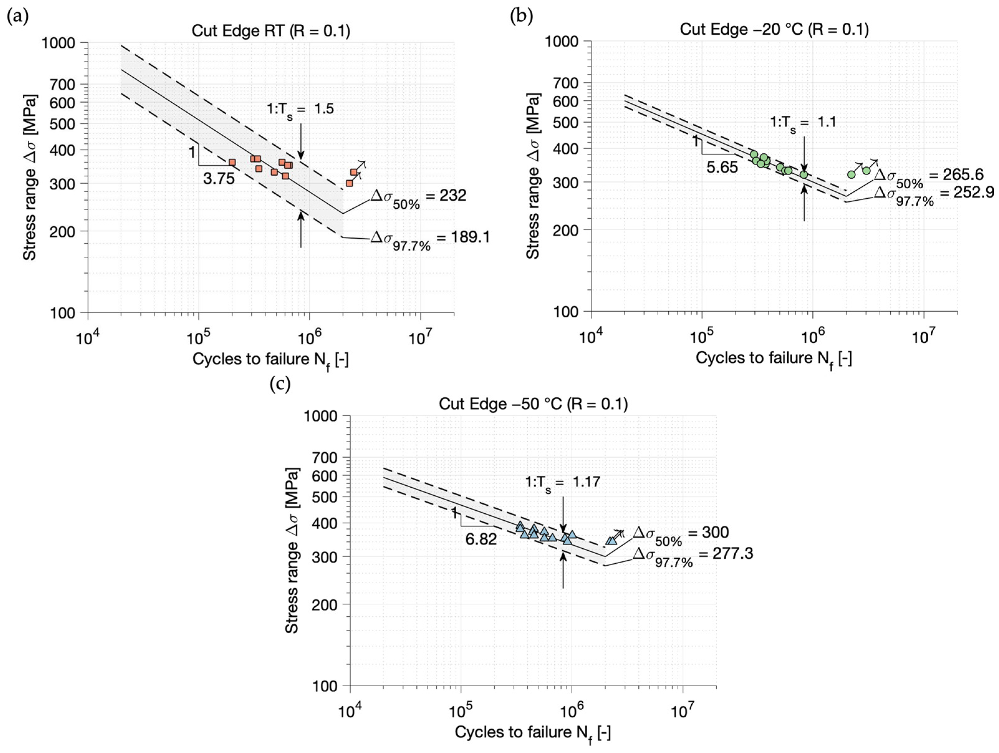
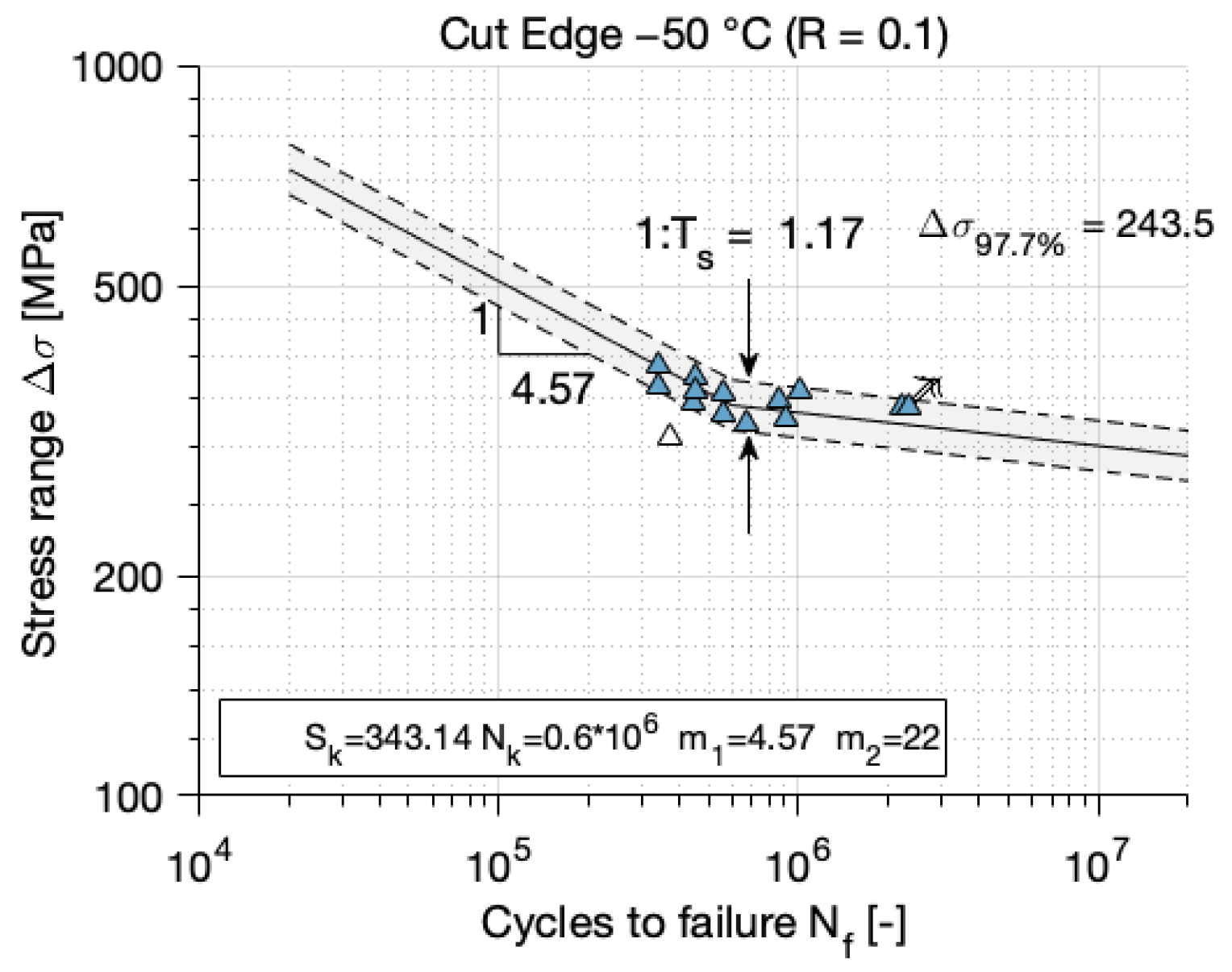
3.1. Statistical Evaluation of Test Results

The fatigue test results are statistically evaluated with two different methods to obtain the mean stress–life (S-N) curve. On the one hand, a linear regression is used to evaluate the S-N curve minimizing the residual sum of squares. In addition to this method, the evaluation is also carried out with the maximum likelihood method. In contrast to a linear regression, the maximum likelihood method takes the runouts into account. Using the maximum likelihood method, a bilinear S-N curve with the highest probability of occurrence is fitted to the data [14].
The method of linear regression accounts for all test data before the knee point. Because of that, the knee point is specified according to the recommendations of the German Welding Society, DVS [14]. The high cycle fatigue regime before the knee point of the S-N curves is represented by the Basquin equation (Equation (1)), which is logarithmized for the common representation of the S-N curves:
lg N = lg N k · Δ σ k m + m · lg Δ σ
With N as the number of cycles, N k as the number of cycles at the knee point, m as the slope, Δ σ as the stress range, and Δ σ k as the stress range at the knee point. By using linear regression [14], the slope in the high cycle fatigue regime was calculated as well as the stress range at 2 · 10 6 cycles for 50% and 97.7% survival probability. This number of cycles reflects the FAT-class values (see, e.g., IIW [4]). Moreover, the band width of the scatter between 97.7% and 2.3% is determined. Within this method, it is assumed that the scatter is represented by the logarithmic normal distribution and is independent of the load level.
In case a specimen did not fail before 2 · 10 6 cycles were reached, those runouts are marked with an arrow in the S-N diagrams. The results for all three test temperatures are shown in the following Figure 5a–c.
When comparing the S-N curves for different temperatures, it can be observed that the fatigue strength increases with decreasing temperature. In addition, the scatter is much higher at RT compared to the sub-zero temperatures. As the slope for RT differs significantly, a linear regression does not seem to be well-suited for data with a high scatter when only a small number of specimens is tested.
Because of that, and the fact that linear regression does not take the runouts into account, the maximum likelihood method was applied to the test results. This method is also recommended by the DVS [14]. With this method, the runouts can be integrated into the evaluation, which can lead to better suited S-N curves for the given data, especially when the number of specimens is small. The method is about to find the bilinear S-N curve with the highest probability of occurrence from the data. As it is shown by Störzel et al. [15], the maximum likelihood method for fatigue test evaluation leads to reliable parameters of the S-N curve. The S-N curve in the maximum likelihood method is represented by a bilinear curve, where both parts of the curve are represented by the Basquin equation (Equation (1)). The curve parameters for the bilinear S-N curve are:
  • Slope in the high cycle fatigue regime m 1 ;
  • Stress range at the knee point S k ;
  • Standard deviation stdv, as a measure of the scatter in the direction of the stress range;
  • Cycles to failure at the knee point N k ;
  • Slope in the long-life fatigue regime m 2 .
The knee point and the slope in the long-life fatigue regime are specified for the calculation and the other three parameters are determined by optimization. The optimization is about to find the highest probability of occurrence for the test points I ( S i ,   N i ). [15]
P t o t , m a x = max ( i = 1 n P i )
In Equation (2), P i represents the probability of a test result that failed or is a runout. As in this method, the scatter is described by the logarithmic normal distribution, and the probability for a failure and a runout are shown in Equations (3) and (4).
P i = 1 , f a i l = 1 s t d v · 2 · π · e 0.5 · ( lg ( y i ) log ( y ( x i ) ) s t d v ) 2 d y
P i = 2 , r u n o u t = 1 2 · π t i e 0.5 t 2 d t
w i t h :   t i = ( lg ( y i ) lg ( y ( x i ) ) ) s t d v
It is further assumed that the scatter is independent of the cycles to failure and that the width of the scatter band is constant at the entire S-N curve. Furthermore, it is a prerequisite for the application of the maximum likelihood method that lines of the same probability meet in the knee point.
In order to find the highest probability of occurrence for the parameter of the S-N curve its natural logarithm is used in the optimization in accordance with [15]. These functions are then called support functions (sup). However, not only the maximum of one support function leads to the best fit S-N curve. The data can be distinguished into three different groups, which depends on the relative position to the knee point:
  • Specimens that failed before the knee point ( N i < N k );
  • Specimens that failed behind the knee point ( N i > N k );
  • Specimens that have not failed (runouts).
For all of the three groups, the support function is different. Because of this, the maximization of the probability of occurrence has to take all support functions into account to find the best fit S-N curve, which is represented by Equation 6.
ln P t o t , max = max ( s u p 1 + s u p 2 + s u p B )
The support functions evaluate the distance between the test point and the S-N curve from the regression line in the direction of the stress range. As the slope of the S-N curve is different before and behind the knee point, this has to be considered for the support functions. Then, the equation for the support functions that are optimized have the following form [14].
F o r   N i < N k             s u p 1 = n 1 ( ( 0.5 · ( lg ( y i ) lg ( y ( x i ) ) ) 2 s t d v 2 ln ( m 1 · s t d v ) )  
F o r   N i > N k             s u p 2 = n 2 ( ( 0.5 · ( lg ( y i ) lg ( y ( x i ) ) ) 2 s t d v 2 ln ( m 2 · s t d v ) )  
F o r   r u n o u t s           s u p B = n B ln 1 2 · π · t i e 0.5 t 2 d x
The parameters that are optimized are stdv, m 1 , and S k . This is conducted by variating these parameters and then calculating the maximum of the support functions according to Equation 6. Due to discontinuity at each test point, the knee point cannot be adopted together with the other parameters [15]. The only way to do this is to optimize the knee point before optimizing the other parameters through finding the knee point with the highest probability of occurrence.
The knee point is determined by variating N k from 0.5 · 10 6 up to 2 · 10 6 in steps of 0.1 · 10 6 . The knee point is selected for which the test results have the greatest probability of occurrence. The fixed slope in the high cycle fatigue regime was set to m 2   = 22, according to the recommendation by DVS [14]. Besides the scatter index between a 97.7% and 2.3% survival probability, the resulting FAT-class value, the stress range for a 50% survival probability at the knee point, and the slope m 1 are calculated. The results of the statistical evaluation with the maximum likelihood method are shown in Figure 6a–c.
The evaluation with the maximum likelihood method confirms the increase in fatigue strength with decreasing temperatures, but the change in the slope is not as significant as in the evaluation with linear regression. Comparing the FAT-class values of the S-N curves, a clear difference was observed between the RT and subzero temperatures. However, the difference in the FAT-class values between −20 °C and −50 °C has become very small using the maximum likelihood method. By comparing the knee point stress range S k , a difference between the test results at sub-zero temperatures is observed. Moreover, only very small changes in the slope and also in the band width of the scatter can be observed for sub-zero temperatures, in comparison to the results with the method of linear regression. This was expected because the failure mechanism is the same as before. In comparison, the slope at RT is less steep and the band width of the scatter is smaller when using the maximum likelihood method.

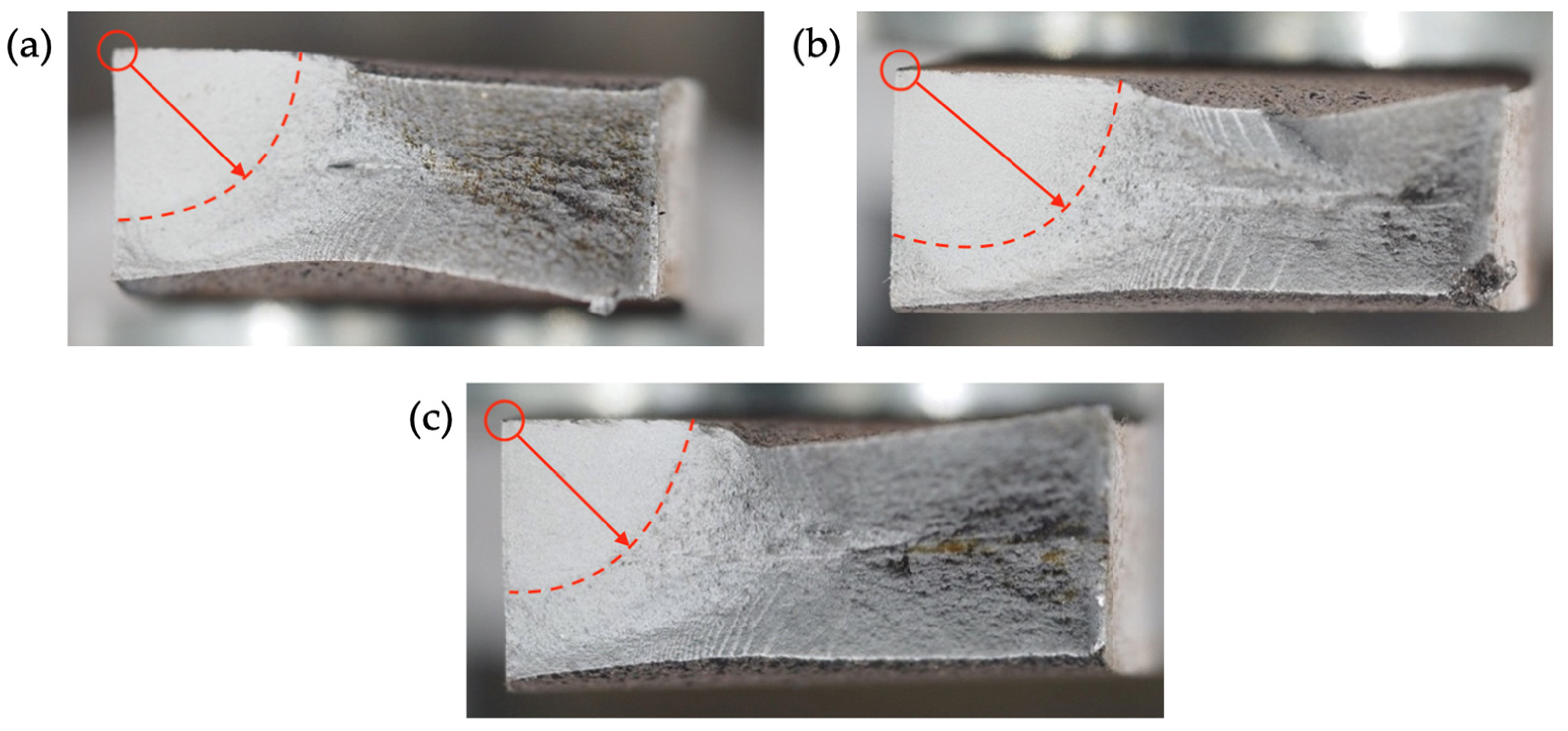
3.2. Fracture Surface

As von Bock und Polach et al. (2022) [16] showed, the position of the crack initiation can have an influence on the fatigue strength of thermal cut edges. The crack initiation at untreated thermal cut edges starts, in most cases, at the corner of the cut edge [17]. A distinction is made between cracks that appear in the grooves on the thermal cut steel surface and cracks that appear in the corner of the cut edges, in case of post-treated specimens in the chamfer [1]. The crack growth can be traced by looking at the fracture surface. Thereby, it is found that all fracture surfaces (independent of the test temperature) show the same position for crack initiation. Figure 7 shows the fracture surface of specimens, which are tested at RT (a), −20 °C (b), and −50 °C (c). The crack initiation starts at the topside corner of the cut edges and propagates to the middle of the fracture surface. When the crack length reaches a certain size, the stiffness of the specimen decreases, and the longitudinal displacement becomes larger due to the constant load amplitude. At pre-set threshold values for displacement and frequency change, the resonance testing machine stops the loading procedure.

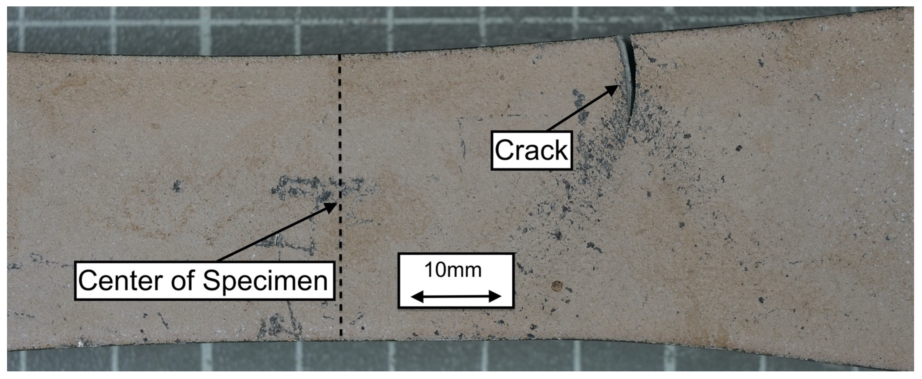
3.3. Influence of the Crack Position.

Corners of the thermal cut steel surface led to local stress concentrations. As those stress concentrations can reduce the lifetime of a specimen significantly, a failure does not only occur at the midsection of a specimen, where the nominal stress is the highest [1]. A specimen where the crack did not occur at the smallest cross section is shown in Figure 8.
The crack positions are measured and the nominal stress according to the local cross section is corrected. This procedure can lead to a sharp drop in the stress range when the crack location is relatively far away from the smallest cross section. The total stress at the crack location is a combination of the nominal stress and the stress concentration and must be higher than the total stress at the smallest cross section. Hence, it can be discussed if the nominal stress at the smallest cross section might not be more representative than the nominal stress at the actual crack location. However, for this study, a statistical evaluation is also carried out for the recalculated test series, where the nominal stresses at the actual crack location are used. The statistical evaluation can become a problem in case single values deviate too much from the others. This can be due to a difference in shape but also to changes in the test conditions. Such outliers lead to a very wide scatter band, which represents the test results incorrectly [18]. To deal with such outliers a graphical analysis is used as there are no methods for a mathematical evaluation [18]. In the test results at −50 °C, one outlier is found. In this case, the crack originates 48 mm out of the middle of the specimen. Plotting the modified stress range of this test next to the S-N curve of the remaining 13 data points, it is seen that the value does not fit in the scatter band. This is shown in Figure 9. Thereby, the statistical evaluation was conducted with the maximum likelihood method with an optimization of the knee point. In case of the tests at −20 °C and RT, no outliers were observed.
In all three of the modified S-N curves, a decrease in the slope exponent is observed. Furthermore, the knee point stress range for a 50% survival probability is lower than in the evaluation with the initial test data. This was expected because the stress ranges are more or less reduced for every data point. However, in total, the difference in the fatigue strength between the sub-zero temperatures remains almost the same. In addition to the evaluation with the maximum likelihood method, a linear regression is used here as well. Thereby, it is observed that the slope differs even more than the results of the initial test data. For example, the slope of the results of the test series at −50 °C has decreased to m = 3.84, which is close to the recommended slopes in the guidelines of DNV (m = 4) [19]. All S-N curve parameters of all test series for both statistical methods are summarized in Table 2.

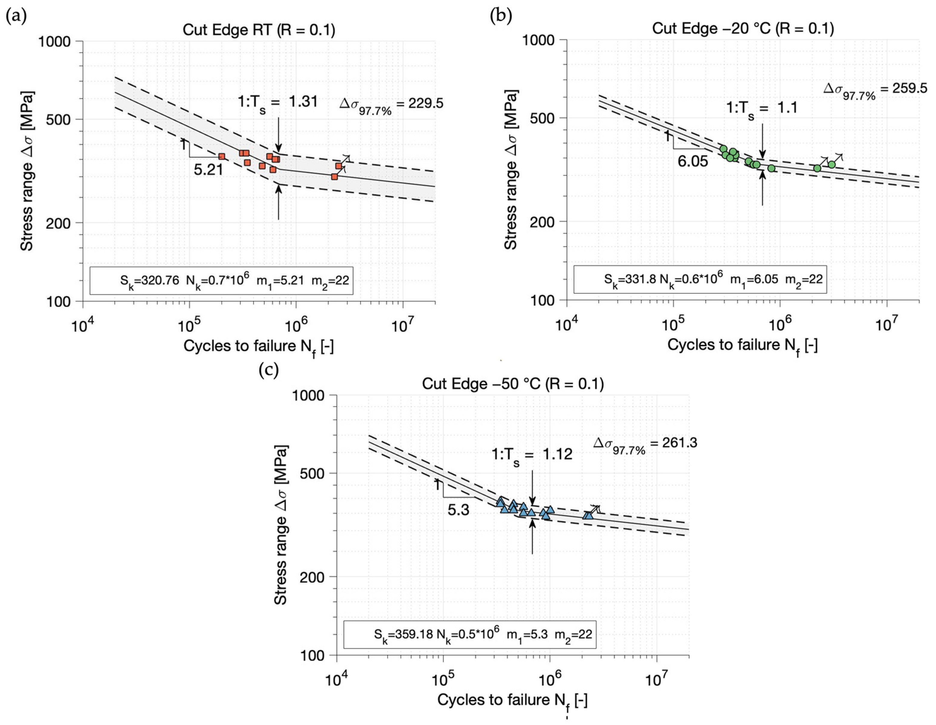
3.4. Linear Regression with Constant Slope

In order to obtain the fatigue performance of thermal cut edge steel at sub-zero temperatures, the best fit S-N curves are evaluated using both the previously described statistical methods. This procedure leads to different slopes for the different test series, which makes the comparison of values complicated, because the difference between the test series depends on the cycles to failure. In order to obtain information about the difference in the stress range, a linear regression is conducted with fixed slopes. Thus, the slopes are set to m = 3, as recommended by the IIW [4], and also m = 4 and m = 3.5, as in the guidelines of DNV [19]. Then, the FAT-class values of each test series are calculated with fixed slopes. The results of the calculation and the corresponding FAT-class values from the guidelines for similar cases are shown in Table 3.
The increase in fatigue strength is represented by the increase in FAT-class values. In Figure 10, the percentage rises to the FAT-class value at RT for the different slopes are shown. Thereby, the increase is the greatest for a fixed slope of m = 3 and smallest for m = 4. However, for all used slopes, a significant increase is observed.

4. Discussion

Fatigue tests of thermal cut steel edges at sub-zero temperatures are conducted and statistically evaluated. Independent to the statistical method, an increase in the fatigue strength of plasma-cut specimens made of AH36 at sub-zero temperatures compared to RT is observed. Despite this, the results evaluated with the linear regression method differ from those evaluated with the maximum likelihood method. The slope of the RT test series evaluated with the method of linear regression is much larger than the slope of the test results from the sub-zero temperatures. The evaluation with the maximum likelihood method shows a smaller slope at RT, which is closer to those at sub-zero temperatures. This is probably caused by the optimized knee point position and the fact that the maximum likelihood method takes the runouts into account. In addition, the number of tested specimens is very limited.
The difference in the statistical methods can also be observed by looking at the band width of the scatter. The tests at RT that were assessed with the linear regression method led to a much wider scatter band than for the maximum likelihood method. This might be caused by the changed knee point position. In comparison to this, the results of the sub-zero tests are not as much influenced by the type of statistical method. So, the difference in the band width of the scatter is relatively small between both methods, like it was also observed in case of the slope. However, with the maximum likelihood method, the difference between the test series is smaller compared to the RT test results with the method of linear regression.
The evaluation with the maximum likelihood method shows a difference in the fatigue strength of the three test temperatures at the knee point, but for the comparison of the fatigue strength, the position of the knee point and the slopes of the curves have to be considered. This can be completed by calculating the stress range of the −20 °C test series at the number of cycles where the −50 °C test series has its knee point. The stress range of the −50 °C test series at 0.5 · 10 6 cycles to failure is then about 18 MPa greater than the stress range of the −20 °C test series, which demonstrates an increase of about 5%. A similar difference in the stress range can be observed at the knee points of the modified S-N curves between the tests at −20 °C and −50 °C. However, this kind of comparison is still full of uncertainties. The difference in the stress range between the test series depends on the cycles to failure, as the curves have different slopes. For example, the FAT-class values of the test series −20 °C and −50 °C only differ by about 2 MPa. Because of that, this way of comparison can only give information about the trend of the curves.
A better way to compare the stress ranges is to use fixed slopes for the evaluation with the linear regression method. Through this, the difference in fatigue strength can be evaluated at any position of the S-N curve. Using fixed slopes of m = 3, m = 3.5, and m = 4, which are in the range given by common guidelines such as IIW or DNV, an increase up to 17.8% for a fixed slope of m = 3 for the −50 °C test series without a stress range correction in comparison to the RT test series is observed. However, the slopes that are evaluated with the maximum likelihood method are less steep than m = 3. Because of that, a fixed slope of m = 4 seems to be better suited for this test series. In that case, the increase from RT to −20 °C (11%) and to −50 °C (15.2%) is smaller, but still significant. Considering the modified S-N curves, where the stress range values are related to the cross section at the crack position, the increase for the tests at −50 °C is smaller, and remains almost the same for the −20 °C test series. In that case, the comparison of the FAT-class values is especially well-suited for the test series at RT and at −50 °C with fixed slopes of m = 3.5 and m = 4, as the evaluated slopes with the linear regression method are for both between these values. Then, an increase from RT to −50 °C of about 13.5% for a slope of m = 4 and 14.9% for a slope of m = 3.5 is calculated.
The FAT-class values at RT, independent of the slope, surpass the FAT-class values of the guidelines. As the test series of sub-zero temperatures shows an increase in fatigue strength, it can be considered that the guidelines are very conservative, especially for thermal cut edges at sub-zero temperatures.
From the literature, it is known that the fatigue of ferritic structural steel undergoes a ductile to brittle transition at the FTT, which is related to a decrease in fatigue strength because the fatigue crack growth is accelerated. However, the results of the fatigue tests show that the fatigue strength of the tested thermal cut edges increased up to the lowest test temperature of −50 °C. This is probably due to the fact that the transition takes place at lower temperatures than those tested here. An indication of this could be found in the fracture surfaces of the tested specimens, so it can be observed that all tested specimens failed in the same ductile manner, independent of the test temperature.
The fatigue strength of thermal cut steel edges in the outer shell of ships, e.g., windows or balcony doors, does not solely depend on the cut edge quality and temperature. Rather, the shape of the cut outs, especially the fatigue critical opening corners, affect the fatigue strength. Thus, the increase in fatigue strength of thermal cut steel edges at sub-zero temperatures found in this study cannot be directly transferred to the cut outs. However, it can be assumed that the fatigue strength of those cut outs increased at sub-zero temperatures tested in this study, but maybe not as much as the test results suggest. More importantly, the test results of this study show that sub-zero temperatures do not pose an increased risk to thermal cut steel edges in terms of fatigue.

5. Conclusions

Thermal cut edge steel specimens of AH36 were tested at sub-zero temperatures and at room temperature. The best fit S-N curves were evaluated with the linear regression and the maximum likelihood method. Furthermore, it was found that the cracks did not always occur at the smallest cross section. Consequently, the local nominal stresses at the actual crack position were calculated and the stress ranges were corrected. With the modified data, the statistical evaluation was repeated. For the comparison of the fatigue strength of the different test series and for a comparison with the guidelines, an evaluation using the linear regression model was also performed with fixed slopes for all test series, both the modified and the not modified ones. The findings of this study are summarized in the following points:
  • After analyzing the statistically evaluated best-fit S-N curves, it is clear that the fatigue strength of thermal cut steel edges of AH36 increase at sub-zero temperatures in comparison to room temperature. This is independent of the statistical method and corresponds to the experience gained with welds at sub-zero temperature [9,10].
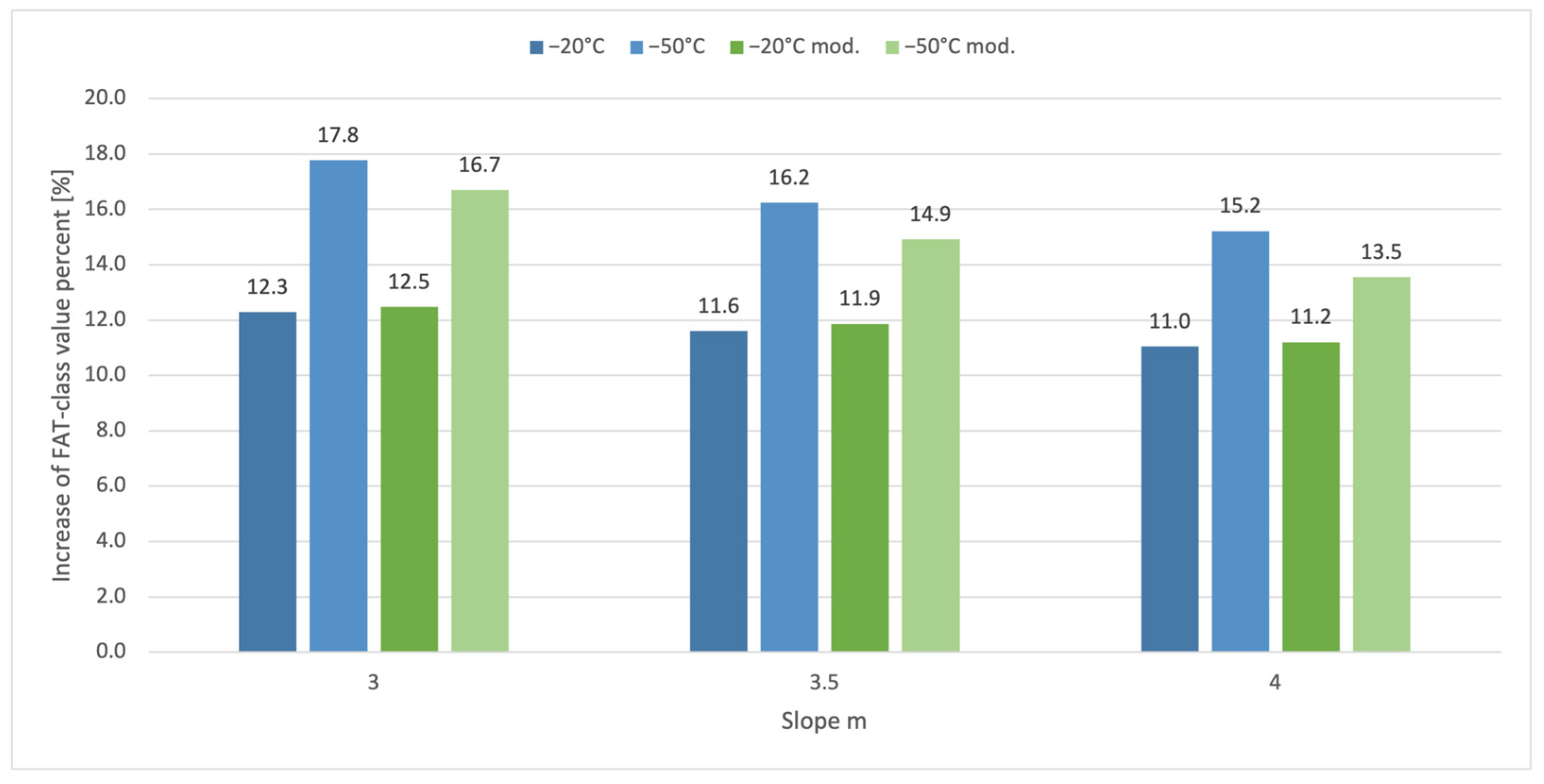
  • A fixed slope of m = 4 seems applicable for the evaluation with fixed slopes as the slopes that are found in the evaluation of the best fit S-N curves are close to that or greater. The modification of the stress range leads to steeper S-N curves, which are even closer to a slope of m = 4.
  • Using fixed slopes shows the increase in fatigue strength in an even clearer manner. The highest increase in fatigue strength evaluated with a fixed slope of m = 4 is about 15.2% at a test temperature of −50 °C and in the case of the modified data, the increase is still about 13.5%.
  • The comparison with the FAT-class values of the design curves of the common guidelines has shown that all test series surpass the FAT-class recommendations. This shows that the design curves are very conservative for thermal cut edges, especially at sub-zero temperatures.
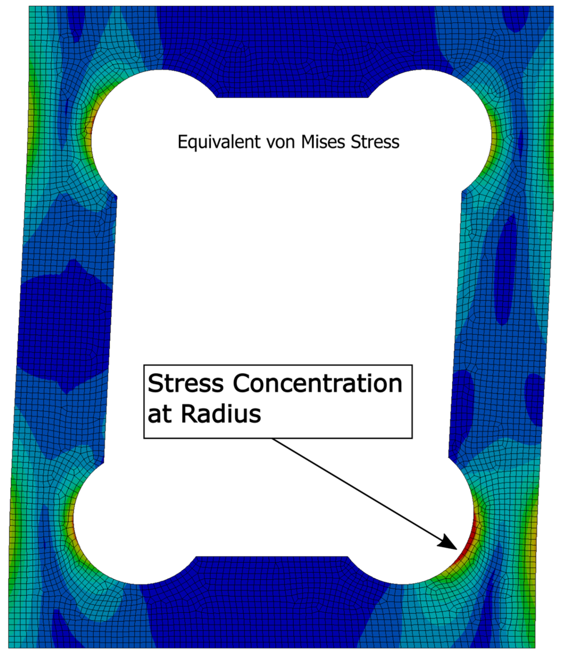
  • A difference in the crack location is not found. All cracks occur in the corner of the cut edges, independent to the test temperature.

Author Contributions

The study was conducted in accordance with the Conceptualization, methodology, software, validation, M.B. (Moritz Braun) and M.B. (Marten Beiler); formal analysis and investigation, M.B. (Marten Beiler); data curation, M.B. (Marten Beiler); writing—original draft preparation, M.B. (Marten Beiler); writing—review and editing, M.B. (Moritz Braun), F.v.B.u.P. and J.-H.G.; visualization, M.B. (Marten Beiler) and T.-N.B.; supervision, M.B. (Moritz Braun) and J.-H.G. All authors have read and agreed to the published version of the manuscript.

Funding

This research received no external funding.

Institutional Review Board Statement

Not applicable.

Informed Consent Statement

Not applicable.

Data Availability Statement

Not applicable.

Conflicts of Interest

The authors declare no conflict of interest.

Nomenclature

SymbolsUnitDescription
T s -Scatter ratio in strength
m -Slope of S-N curve in linear regression
m 1 -Slope before the knee point in maximum likelihood method
m 2 -Slope behind the knee point in maximum likelihood method
N f CyclesCycles to failure
N k CyclesNumber of cycles at knee point
σ MPaStress range
σ k MPaStress range at the knee point
R -Stress ratio
S k MPaStress range at knee point
P t o t , m a x -Highest probability of occurrence
P i -Probability of occurrence for one test point
P i = 1 , f a i l -Probability of occurrence for a failure
P i = 2 , r u n o u t -Probability of occurrence for a runout
s t d v -Standard deviation in the direction of the stress range

Abbreviations

FDBTFatigue ductile–brittle transition
FTTFatigue transition temperature
RTRoom temperature

References

  1. von Bock und Polach, F.; Kahl, A.; Braun, M.; von Selle, H.; Ehlers, S. Analysis of governing parameters on the fatigue life of thermal cut edges. In Proceedings of the International Conference on Ships and Offshore Structures ICSOS, Orlando, FL, USA, 4–8 November 2019. [Google Scholar]
  2. Lipiäinen, K.; Ahola, A.; Skriko, T.; Björk, T. Fatigue strength characterization of high and ultra-high-strength steel cut edges. Eng. Struct. 2021, 228, 111544. [Google Scholar] [CrossRef]
  3. Diekhoff, P.; Hensel, J.; Nitschke-Pagel, T.; Dilger, K. Fatigue Stregth of Thermal Cut Edges-Influence of ISO 9013 Quality Groups; XIII-2687-17; International Institute of Welding: Liguria, Italy, 2017. [Google Scholar] [CrossRef]
  4. Hobbacher, A.F. Recommendations for Fatigue Design of Welded Joints and Component, 2nd ed.; Springer International Publishing: Cham, Switzerland, 2016. [Google Scholar]
  5. Walters, C.; Alvaro, A.; Johan, M. The effect of low temperatures on the fatigue crack growth of S460 structural steel. Int. J. Fatigue 2016, 82, 110–118. [Google Scholar] [CrossRef]
  6. Von Bock und Polach, F.; Klein, M.; Kubiczek, J.; Kellner, L.; Braun, M.; Herrnring, H. State of the art and knowledge gaps on modelling structures in cold regions. In Proceedings of the ASME 2019 38th International Conference on Ocean, Offshore and Arctic Engineering, Glasgow, UK, 9–14 June 2019. [Google Scholar] [CrossRef]
  7. Wallin, K. A Simple Theoretical Charpy-V–KIc correlation for irradiation embrittlement. ASME-PVP 1989, 170, 93–100. [Google Scholar]
  8. Dzioba, I.; Lipiec, S. Fracture Mechanism of S355 Steel–Experimental Research, FEM Simulation and SEM Observation. Materials 2019, 12, 3959. [Google Scholar] [CrossRef] [PubMed]
  9. Braun, M.; Scheffer, R.; Fricke, W.; Ehlers, S. Fatigue strength of fillet-welded joints at subzero temperatures. Fatigue Fract. Eng. Mater. Struct. 2020, 43, 403–416. [Google Scholar] [CrossRef]
  10. Braun, M.; Milaković, A.; Ehlers, S.; Kahl, A.; Willems, T.; Seidel, M.; Fischer, C. Sub-zero temperatures fatigue strength of Butt-welded normal and high-strength steel joints for ships and offshore structures in arctic regions. In Proceedings of the ASME 2020 39th International Conference on Ocean, Offshore and Arctic Engeneering, Virtual, 3–7 August 2020. [Google Scholar] [CrossRef]
  11. Sperle, J.-O. Influence of Parent Metal Strength on the Fatigue Strength of Parent Material with Machined and Thermally Cut Edges; IIW Document XIII-2174-07; International Institute of Welding: Paris, France, 2007. [Google Scholar]
  12. Grimm, J.-H.; Castro, J.; von Selle, H.; Braun, M.; von Bock und Polach, F.; Ehlers, S.; Hensel, J.; Hesse, A.-C.; Dilger, K. The influence of edge treatment on fatigue behavior of thermal cut edges. In Proceedings of the ASME 2022 41st International Conference on Ocean, Offshore and Arctic Engineering, Hamburg, Germany, 5–11 June 2022. [Google Scholar]
  13. Deutsche Fassung EN ISO 9013:2017; Thermisches Schneiden–Einteilung Thermischer Schnitte–Geometrische Produktspezifikation und Qualität (ISO 9013:2017). Deutsches Institut für Normung: Berlin, Germany, 2017.
  14. Merkblatt DVS 2403. Empfehlung für die Durchführung, Auswertung und Dokumentation von Schwingfestigkeitsversuchen an Schweißverbindungen Metallischer Werkstoffe; Deutscher Verband für Schweißen und verwandte Verfahren: Düsseldorf, Germany, 2019.
  15. Störzel, K.; Baumgartner, J. Statistical Evaluation of Fatigue Tests Using Maximum Likelihood; Walter de Gruyter GmbH: Berlin, Germany; Boston, MA, USA, 2021. [Google Scholar] [CrossRef]
  16. von Bock und Polach, F.; Kahl, A.; Braun, M.; Sperle, J.-O.; von Selle, H.; Ehlers, S. Analysis of the scatter in fatigue life testing of thick thermal cut plate edges. Ships Offshore Struct. 2023, 18, 217–230. [Google Scholar] [CrossRef]
  17. Diekhoff, P.; Hensel, J.; Nitschke-Pagel, T.; Dilger, K. Investigation on Fatigue Strength of Cut Edges of High Strength Steels (S355M, S690Q); IIW Annual Assembly, Document XIII—2732-18; University of Braunschweig: Braunschweig, Germany, 2018. [Google Scholar]
  18. Haibach, E. Betriebsfestigkeit, Verfahren und Daten zur Bauteilberechnung; Springer: Berlin/Heidelberg, Germany, 2006. [Google Scholar]
  19. DNVGL. Fatigue Assessment of Ship Structures; DNVGL-CG-0129; Class Guideline, Edition October 2015; DNV GL AS: Oslo, Norway, 2015. [Google Scholar]
Figure 1. Stress concentration in a thermal cut radius of a typical opening in a ship structure.
Jmse 11 00346 g001
Figure 2. Specimen dimension and cut condition, modified from [12].
Jmse 11 00346 g002
Figure 3. Microstructure of polished inclined cross section. Top side edge with sharp corner (flame entry) and more round edge on bottom side.
Jmse 11 00346 g003
Figure 4. Temperature chamber that covers the clamping jaws of the horizontal testing machine (a) and uniaxial loaded specimen (b).
Jmse 11 00346 g004
Figure 5. S-N curves of AH36 cut edges from linear regression for RT (a), −20 °C (b) and −50 °C (c).
Jmse 11 00346 g005
Figure 6. S-N curves of AH36 cut edges from maximum likelihood method for RT (a), −20 °C (b) and −50 °C (c).
Jmse 11 00346 g006
Figure 7. Fracture surface of AH36 cut edges tested at temperatures of RT (a), −20 °C (b) and −50 °C (c), with location of crack initiation and direction of crack propagation.
Jmse 11 00346 g007
Figure 8. Specimen where the crack position is not at the smallest cross section.
Jmse 11 00346 g008
Figure 9. S-N curve of AH36 cut edges for test results at −50 °C with modified stress ranges evaluated with the maximum likelihood method. The white triangle shows the outliner.
Jmse 11 00346 g009
Figure 10. Increase in the FAT-class value in percent of tested AH36 cut edges at sub-zero temperatures compared to RT and of modified test series compared to RT modified. In the modified test series, the nominal stresses in the cross sections at the actual crack locations are used instead of the nominal stresses at the smallest cross sections.
Jmse 11 00346 g010
Table 1. Chemical composition of alloying elements in % and observed mechanical properties of AH36 steel [12].
CSiMnPSAlN
0.090.251.160.0170.0060.0280.007
CrCuNiTiVNbMo
0.090.220.120.0010.0010.0240.001
CEVTensile Strength R m (MPa)Yield Strength R e h (MPa)Failure Strain (%)
0.3253842329.2
Table 2. S-N curve parameter evaluated with linear regression and with maximum likelihood method for all test series. “mod.” refers to the actual crack position, i.e., the modified stress.
Statistical MethodLinear RegressionMaximum Likelihood Method
Parameter m 1 : T s FAT (MPa) m 1 m 2 1 : T s N k S k (MPa) FAT (MPa)
RT3.751.5189.15.21221.31 0.7 · 10 6 320.76229.5
−20 °C5.651.1252.96.05221.1 0.6 · 10 6 331.8259.5
−50 °C6.821.17277.35.3221.12 0.5 · 10 6 359.18261.3
RT mod.3.571.51179.34.8221.33 0.7 · 10 6 310.11216.5
−20 °C mod.5.121.12237.95.26221.13 0.6 · 10 6 323.92242.2
Table 3. FAT-class values for test series RT, −20 °C, and −50 °C, and for test series with modified stress range values with different fixed slopes and FAT-class values from guidelines [4,19].
Test SeriesRT (MPa)−20 °C (MPa)−50 °C (MPa)RT Mod. (MPa)−20 °C Mod. (MPa)−50 °C Mod. (MPa)Guideline (IIW Case No. 122, DNV Case B2 and C)
m = 3162181.9190.8158.7178.5185.2125 (IIW)
m = 3.5181202.0210.4177.0198.0203.4125 (DNV)
m = 4196.5218.2226.4191.9213.4217.9140 (DNV)
Disclaimer/Publisher’s Note: The statements, opinions and data contained in all publications are solely those of the individual author(s) and contributor(s) and not of MDPI and/or the editor(s). MDPI and/or the editor(s) disclaim responsibility for any injury to people or property resulting from any ideas, methods, instructions or products referred to in the content.

