Research on Black-Box Modeling Prediction of USV Maneuvering Based on SSA-WLS-SVM

Abstract

Unmanned surface vessels (USVs) are required to perform motion prediction during a task. This is essential for USVs, especially when conducting motion control, and this work has been proven to be complicated. In this paper, an off-line black box modeling method for USV maneuvering, the Sparrow search algorithm-based weighted-least-squares support vector machine (SSA-WLS-SVM) was proposed to recognize the motion model of a USV. Firstly, the construction of the USV test platform and the processing process of the experimental data were introduced, the correctness of the MMG model was verified using a comparison of the test data and the simulation results, and then the MMG model was used to produce sample data later. To improve the stability and robustness of LS-SVM, weighted least squares and SSA were introduced to perform the optimization of the parameters of the algorithm and its kernel function. Then, the random maneuvering dataset was obtained using simulation on the MMG model, which was then preprocessed and used for training the black-box model. To verify the generalization ability of the identified model, the black-box model was used for comparison analysis between motion prediction with the proposed model and maneuvering test on the USV platform in a scenario different from the training data.

1. Introduction

The Unmanned Surface Vehicle (USV), which can be equipped with a positioning system, automatic identification system (AIS), communication system, water quality detection system, and other systems, has been widely used in the fields of hydrological and geographic exploration, marine weather forecast, coastal port security, and marine environment monitoring due to its low cost and fast speed [1,2,3]. The USV is greatly affected by disturbance of the sea environment, especially waves, which has a significant influence on the stability of its motion control system. Accurate motion prediction is the basis for a USV to perform its maneuverability, so motion prediction is essential for USV navigation control [4,5]. Motion modeling plays a vital role in research on USV motion prediction in a real water scenario. At present, the methods for ship motion modeling are mainly divided into two types: the method based on Computational Fluid Dynamics (CFD) and the modeling method based on the system identification.

In the CFD method, the hydrodynamic force on a USV can be calculated to predict the USV motion. However, the method is usually developed on the basis of the assumption of non-viscous flow, and the calculation accuracy is affected. The viscous flow method in CFD can be used to obtain details of the flow field and hydrodynamic dynamics of the ship, but the calculation is time-consuming, and the convergent solution is often difficult to obtain [5]. Jiang Fan et al. [6] conducted a CFD simulation on the maneuverability of an asymmetric catamaran, calculating the ±15° and ±25° turning maneuver simulations and the 25°/25° zigzag maneuver simulation under different initial steering directions. However, the layout of the asymmetric catamaran involved in the calculation was not perfect, and the self-navigation experiment was not conducted for comparison. Liu et al. [7] used the commercial software STAR-CCM+ to perform a virtual model test to obtain the hydrodynamic coefficients of the standard KCS model. The hydrodynamic derivatives obtained were used in the Abkowitz model to predict the maneuvering performance of the KCS model, but the calculation accuracy was greatly affected by the experience of software users.

The commonly used modeling methods based on system identification include white-box modeling and black-box modeling. White-box modeling is also known as mechanism modeling, which means the mechanism of the system is clear and the structure of the model is generally fixed. The parameters in the white-box model are hydrodynamic coefficients that need to be identified, which can be obtained using system identification and then substituted into the ship’s maneuvering motion equation for maneuvering motion prediction [8]. The Nomoto model is a very simple ship maneuvering motion model which needs only several KT parameters to roughly show the relationship between steering and heading. Carrillo et al. [9] performed a modeling of ship motion based on the Nomoto control model and adopted the least square method to identify the KT parameters. Compared with the Nomoto model, the ship motion model based on the Abkowitz model and MMG (Maneuvering Modeling Group) model can obtain higher prediction accuracy. The team of Professor Zou Zaojian [9,10,11] applied the SVM method to identify the hydrodynamic derivative and hydrodynamic distance in the Abkowitz model based on the global model and forecast the ship’s maneuvering motion. Xu et al. proposed an optimal truncated LS-SVM [12,13] and verified the method using free-run tests [14,15], but the scale effect was ignored in the study. The literature [16] describes the 3-DOF MMG mathematical model of the adaptive modular waveship (WAM-V). The model test and the identification of the system are both used to calculate the maneuvering coefficient of the WAM-V. The MMG model in the simulation shows a satisfactory uniformity in the characteristics of linear and turning. However, problems such as serious ocean disturbance and power shortages remain unresolved. Luo W et al. [17] proposed a two-layer feedforward neural network to identify the nondimensional fluid dynamics derivative in the linear MMG model, and the stability of the estimated parameters was verified. The MMG model is simplified too much, so the accuracy of parameter identification is reduced.

In the above identification work using the white-box model, the task is to identify the coefficients or parameters in the model, so the accuracy of identification is limited by the mathematical model [18]. On the one hand, the use of a fixed, linear, and time-invariant mathematical model of ship maneuvering motion leads to poor generalization [18,19], which means that complex nonlinear characteristics of the actual ship motion cannot be obtained; on the other hand, the use of a complex, nonlinear mathematical model needs to identify too many parameters, which demands a large number of high-quality sample data [18,19]. In addition, the calculation accuracy of hydrodynamic parameters of the hull, propeller, and rudder will also affect the accuracy of the motion prediction. In addition, in the whole life-cycle of a ship, errors in ship design and manufacturing, equipment abrasion during the maneuvering of a ship, changes in the ocean environment, and ship load will also lead to the imprecision of the ship motion model. The inaccuracies of all the above limit the use of the white-box model in motion prediction. However, at the same time, using the white-box model in research is helpful to improve the original mathematical model. Bonci et al. [20] improved the completely nonlinear Abkovitz model by identifying CFD free-run simulations of the USV model by obtaining large amounts of data (less noisy than experimental data) and using these data to constrain the optimization process. The purpose of this work is to eliminate the typical characteristic noise of outdoor pool experimental data using high-precision CFD data.

The black-box model does not need to clarify the mechanism and structure of the system but only needs to describe the functional relationship between input and output. Therefore, the physical meaning of the black-box model is usually not clear, but it does not affect the regression prediction ability of the model [6,21]. In the case of imprecise ship parameters and uncertain structural forms of ship maneuvering motion mathematical models, black-box modeling is a satisfactory choice for ship maneuvering motion modeling based on automatic control [18,19]. Owning to Artificial Neural Networks (ANNs) and Support Vector Machines (SVMs) having strong advantages in identifying nonlinear systems, SVM can be used to construct a black-box model to describe the nonlinear mapping relationship in ship maneuvering motion.

In recent years, Professor Zou Zaojian et al. [22,23,24] have done a lot of work in black-box modeling including a black-box modeling method based on the BP neural network proposed for the 3-DOF ship maneuvering motion, and the network-based model has the potential to be used as a control model or state observer in the field of ship motion control; a fully connected neural network used to establish a black box model of the 3-DOF ship maneuvering motion, and the model can be identified and verified with only three maneuvering operations, but environmental interference is not considered in the work; a black-box offline modeling method, multi-output support vector machine (MO-v-SVR), is also proposed. The traditional v-SVR is optimized in terms of calculation efficiency and maneuverability, but external interference of environmental factors that may affect the dynamic characteristics of the ship is not considered. Liu et al. [25] developed three different identification frameworks in the literature based on KVLCC2, which are the parametric grey-box model, the nonparametric grey-box model, and the black-box model based on Bayesian regression. Using the experimental data, the black-box model was verified to have a stronger generalization ability compared with SVM and ANN, due to the introduction of prior knowledge in the loss function. However, the training set used in the paper was based on regular waves, which may not perform well under other wave conditions. Prateek Gupta et al. [26] used several machine learning (ML) methods to discover the trend of variation in the hydrodynamic performance of the vessel over time. The study indicates that the artificial neural network (ANN) model performed the best in the prediction, but the nonlinear principal component regression (NL-PCR) and nonlinear partial least squares regression (NL-PLSR) were also not bad, demonstrating that simple interpretable ML models such as NL-PCR and NL-PLSR can be used to optimize complex black-box models when extremely high accuracy is not required. However, it is difficult to apply the method in scenarios with too much noise.

In this paper, a black-box modeling method based on the weighted least squares support vector machine (WLSSVM) is proposed for modeling 3-DOF ship maneuvering motion. By using the regression based on a small sample set, the tedious iteration of the hydrodynamic coefficient in white-box modeling can be avoided, and the convergence and robustness of the model are improved. In the process of model identification, in order to obtain the optimal structural parameters in the WLSSVM, the Sparrow search algorithm (SSA) was introduced into the WLSSVM, and the parameters of the algorithm and its kernel function were optimized. To test the performance of the proposed WLSSVM model, the maneuvering motion of the ship is simulated and predicted in the turning test and the arbitrary steering test, and the predicted results are compared with the actual test data.

The work that has been done in this paper can be listed as the following three steps:

(1)

To obtain maneuvering data samples that meet the condition of regression processing.

(2)

Determine the black-box regression model and train the model using the dataset obtained above to obtain the nonlinear relationship between the input and output samples.

(3)

To predict the output of the test set using the trained black-box model and to compare the output with the actual results to verify the generalization of the model.

The paper is organized as follows: the first Section briefly describes the problems to be solved in ship motion prediction. The second Section describes the construction of the USV test platform and the processing process of the experimental data, the correctness of the MMG model is verified through the comparison of the test data, and the simulation results, and then the MMG model can be used to produce sample data later. In Section 3, the SSA-WLS-SVM regression prediction method is briefly derived. In Section 4, the random maneuvering dataset is obtained using simulation of the MMG model and then preprocessed and used for training the black-box model, and the generalization of the model was verified using simulation.

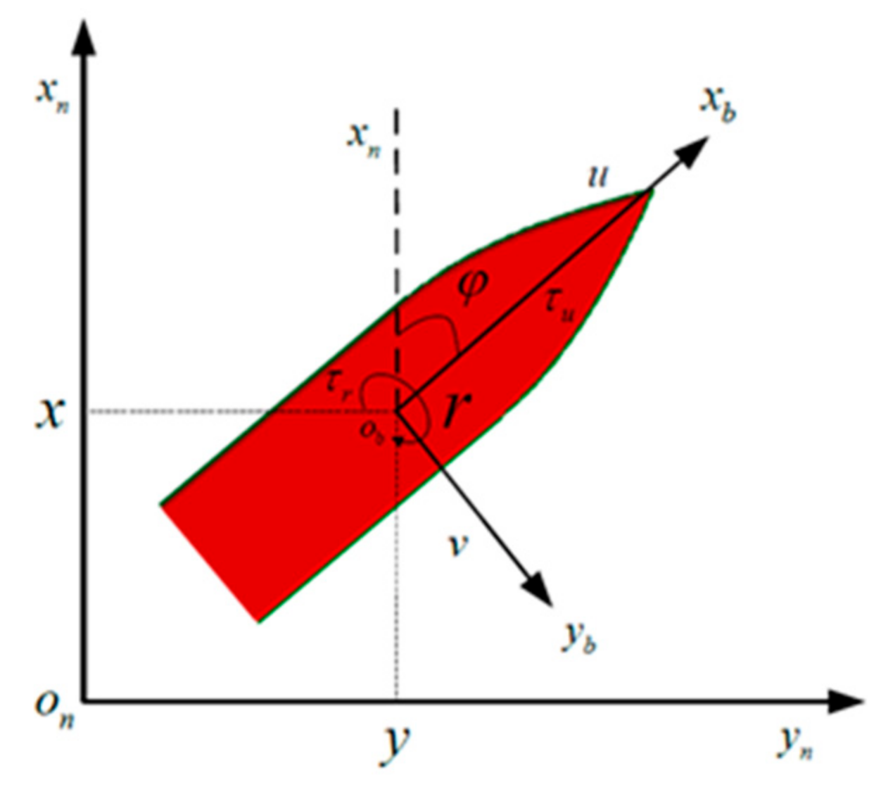
2. Description of a Ship Motion Prediction Problem

The Materials and Methods should be described with sufficient details to allow others to replicate and build on the published results. Please note that the publication of your manuscript implicates that you must make all materials, data, computer code, and protocols associated with the publication available to readers. Please disclose at the submission stage any restrictions on the availability of materials or information. New methods and protocols should be described in detail while well-established methods can be briefly described and appropriately cited.

In this paper, a 3-DOF MMG model is used to describe the USV motion. The geodetic coordinate system $o\text{-}{x}_0{y}_0{z}_0$ and the random body coordinate system $o\text{-}{x}_b{y}_b{z}_b$, are shown in Figure 1, where the x-axis in the random body coordinate system $o\text{-}{x}_b{y}_b{z}_b$ points to the bow and the y-axis points to the starboard.

This nonlinear relationship between the input and output samples is given as follows:

$$\mathit{y}=\rho \left(\mathit{x}\right)$$

(1)

where ρ(⋅) is a non-linear vector function; x is the input sample matrix composed of input sample vectors ${\mathit{x}}_{\mathit{i}}$, $\mathit{x}={\left[{\mathit{x}}_{\mathbf{1}},\cdots {\mathit{x}}_{\mathit{i}},\cdots ,{\mathit{x}}_{\mathit{N}}\right]}^T$; ${\mathit{x}}_{\mathit{i}}$ is the input sample vector, ${\mathit{x}}_{\mathit{i}}=\left[u_i,v_i,r_i,{\delta }_i\right]$; y is the output sample matrix composed of the output sample vector, $\mathit{y}={\left[{\mathit{y}}_{\mathbf{1}},\cdots {\mathit{y}}_{\mathit{i}},\cdots ,{\mathit{y}}_{\mathit{N}}\right]}^T$; and ${\mathit{y}}_{\mathit{i}}$ is the output sample vector, ${\mathit{y}}_{\mathit{i}}=\left[{\dot{u}}_i,{\dot{v}}_i,{\dot{r}}_i\right]$. The superscript T represents the transpose of the matrix. $i$ represents the input or output vector corresponding to the $i_{th}$ data point, and $i=1,2,\cdots ,N$, $N$ is the number of sample points in sample set S. $u$ is the longitudinal velocity, $v$ is the lateral velocity, and $r$ is the steering angular speed.

Briefly speaking, the USV maneuvering forecast is to calculate the $\left[u,v,r\right]$ at the next moment based on the motion and maneuvering information at this moment, that is $\left[u,v,r,\delta \right]$. When some USV parameters are missing or inaccurate, where the motion cannot be accurately predicted with a white-box model, it is appropriate to obtain the mathematical relationship of the input and output with the black-box model.

3. Black-Box Model Training Data Acquisition

The following processes are performed to obtain the training data for the black-box modeling:

(1)

A 3-DOF MMG motion simulation in typical scenes was conducted;

(2)

A test platform was established for test verification (including filtering of test data);

(3)

The test date was compared with the MMG simulation date to verify the accuracy of the MMG model;

(4)

The MMG model was used to produce training data.

3.1. MMG Modeling for Simulation Purposes

According to the requirements of maneuvering and motion characteristics of USVs, the RANS method is used to calculate the maneuvering hydrodynamic forces of a USV in still water, and the MMG model is established. Using the established model, the maneuvering and motion characteristics of a USV in still water are analyzed by solving the ship motion equation.

It mainly includes two works: (1) the hydrodynamic calculation method and modeling of the USV; and (2) the maneuvering and motion characteristics of the USV.

3.1.1. Static Hydrodynamic (Moment) Modeling

The 3-DOF MMG motion model of the USV horizontal plane is established as follows [27]:

$$\left\{\begin{array}{l}\dot{x}=ucos\phi -vsin\phi \\ \dot{y}=usin\phi +vcos\phi \\ \dot{\phi }=r\\ \dot{u}=\frac{1}{m+m_x}\left[\left(m+m_y\right)rv+X_H+X_P+X_R\right]\\ \dot{v}=\frac{1}{m+m_y}\left[-\left(m+m_x\right)rv+Y_H+Y_P+Y_R\right]\\ \dot{r}=\frac{1}{I_{zz}+J_{zz}}\left(N_H+N_P+N_R\right)\end{array}\right.$$

(2)

where X, Y, and N represent hydrodynamic forces and moments, while the subscripts H, P, and R represent the hull, propeller, and rudder, respectively. x and y are the coordinates of the USV in the geodetic coordinate system, φ is the angle of the bow, $m_x$ is the additional longitudinal mass, $m_y$ is the additional transverse mass, and $I_{zz}$ is the inertia moment of yaw. $J_{zz}$ is the additional moment of inertia in yaw.

For the modeling of hydrostatic hydrodynamic (moment), the approximate model for calculating $X_{calm}$, $Y_{calm}$, $N_{calm}$ was established using the MMG model, the hydrostatic manipulates the hydrodynamic force, due to the linear superposition of the details (moments) acting on the hull, propeller, and rudder, which ignores the transverse force and turning moment acting on the propeller.

$$\left\{\begin{array}{c}{X}_{calm}=X_H+X_P+X_R\\ Y_{calm}=Y_H+Y_R\\ N_{calm}=N_H+N_R\end{array}\right.$$

(3)

The force acting on the hull is approximate to the hydrodynamic derivative, $X_H$, $Y_H$, $N_H$ and can be expressed as:

$$\left\{\begin{array}{c}{X}_H=X_0+X_u\Delta u+X_{uu}{\left(\mathsf{\Delta }u\right)}^2+X_{uuu}{\left(\mathsf{\Delta }u\right)}^3+X_{vv}{v}^2+X_{rr}{r}^2+X_{vr}vr\\ Y_H=Y_{v}v+Y_{vvv}{v}^3+Y_{\dot{v}}\dot{v}+Y_{r}r+Y_{rrr}{r}^3+Y_{\dot{r}}\dot{r}+Y_{vrr}v{r}^2+Y_{vvr}{v}^{2}r\\ N_H=N_{v}v+N_{vvv}{v}^3+N_{\dot{v}}\dot{v}+N_{r}r+N_{rrr}{r}^3+N_{\dot{r}}\dot{r}+N_{vrr}v{r}^2+N_{vvr}{v}^{2}r\end{array}\right.$$

(4)

where $\mathrm{\Delta }u=u-u_0$ is the speed difference of the ship relative to the initial ship speed; and $-X_0$ is the resistance when the speed of ship is $u_0$.

Based on the assumption of fluid incompressibility, the governing equations (continuity equations and RANS equations) for manipulating fluid flow around the USV are as follows:

$$\frac{\partial U_i}{\partial x_i}=0$$

(5)

$$\begin{gathered} \frac{\partial U_i}{\partial t}+\frac{\partial \left(U_i{U}_j\right)}{\partial x_j}=f_i-\frac{1}{\rho }\frac{\partial p}{\partial x_i}+\frac{\partial }{\partial x_j}\left[\nu \left(\frac{\partial U_i}{\partial x_j}+\frac{\partial U_j}{\partial x_i}\right)-\overline{U_i^{\prime }{U}_j^{\prime }}\right] \\ -\left(\frac{\partial u_i}{\partial t}+{\epsilon }_{ijk}{\Omega }_j{u}_k\right)-{\epsilon }_{ijk}{\Omega }_j{\epsilon }_{kmn}{\Omega }_m{x}_n-2{\epsilon }_{ijk}{\Omega }_j{U}_k-{\epsilon }_{ijk}\frac{\partial {\Omega }_j}{\partial t}{x}_k \end{gathered}$$

(6)

where $U_i$ is fluid velocity; $p$ is for pressure; $\nu$ is the dynamic viscosity coefficient; $x_i$ is the coordinate; $u_i=\left(u,v,w\right)$ is the speed of the ship; ${\Omega }_j=\left(p,q,r\right)$ is the angular velocity of ship rotation; $-\rho \overline{U_i^{\prime }{U}_j^{\prime }}$ is Reynolds stress; $\rho$ is the density; $f_i$ is volume force; and ${\epsilon }_{ijk}$ is the permutation symbol.

Compared with the RANS equation in the geodetic coordinate system, the RANS equation in the horizontal shipboard coordinate system, Equation (6), has four more inertia force terms in the second row. In this project, based on OpenFOAM, a program module for the calculation of these four terms was developed to solve the RANS equation in the horizontal shipboard coordinate system, to achieve the calculation of the hydrodynamic force of the vessel controlled by constrained motion.

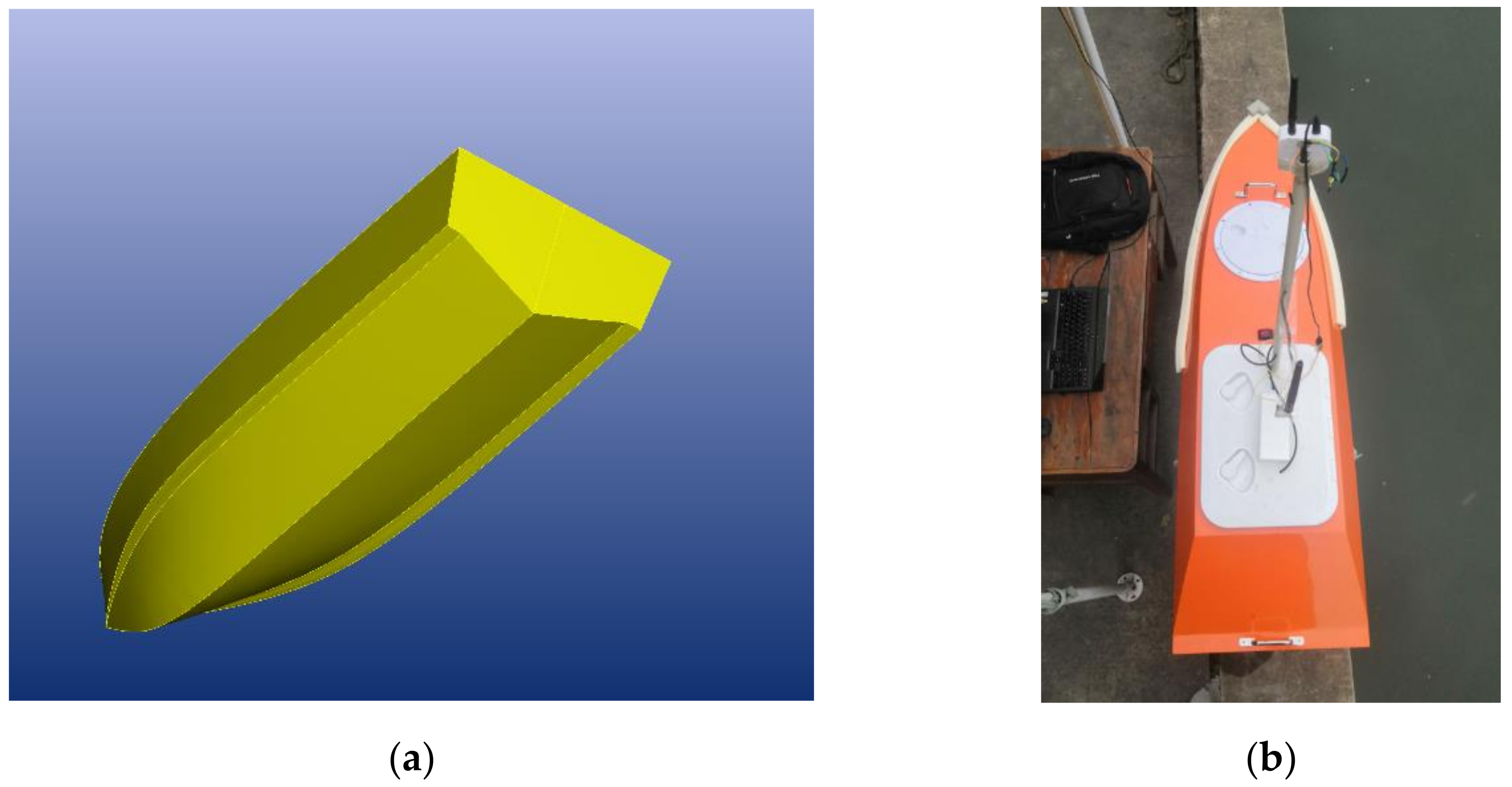
3.1.2. Calculation Object

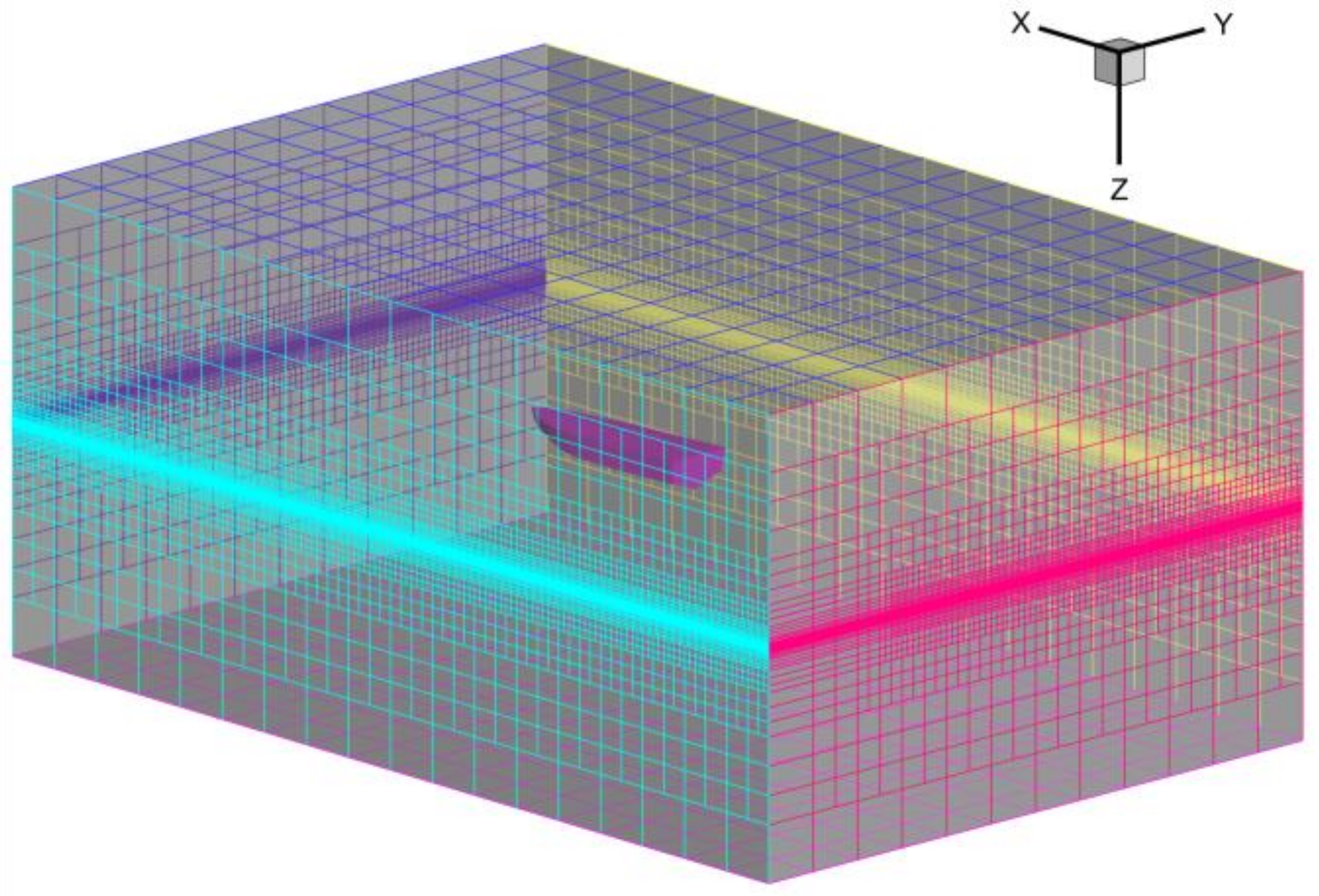
The geometric shape and model of the USV are shown in Figure 2. The main dimensions of the ship model are shown in

Table 1. Main scale of the unmanned boat.

Project	Value
Hall
$L_{pp} \left(m\right)$	1.5
$B \left(m\right)$	0.444
$d \left(m\right)$	0.107
$C_B$	0.395
$x_G \left(m\right)$	−0.12
$z_G \left(m\right)$	−0.3
$I_z \left(kg·m^2\right)$	3.947
$I_x \left(kg·m^2\right)$	0.35
Propeller
$D_p \left(m\right)$	0.05
$Z_P \left(\mathrm{number}\right)$	5
Rudder
$A_R$ $\left(m^2\right)$	0.001675
$H_R \left(m\right)$	0.05

.

3.1.3. Compute Grid

The calculation region is limited to a rectangular solid, whose ranges are $-4.5\le x/L_{pp}\le 3$, $-1\le y/L_{pp}\le 1$, and $-1\le z/L_{pp}\le 1.0$. The commercial software Hexpress is used to generate unstructured cutting grids in the calculation area. The calculation grid in the calculation area is shown in Figure 3, and the number of grid cells is about 1.6 million.

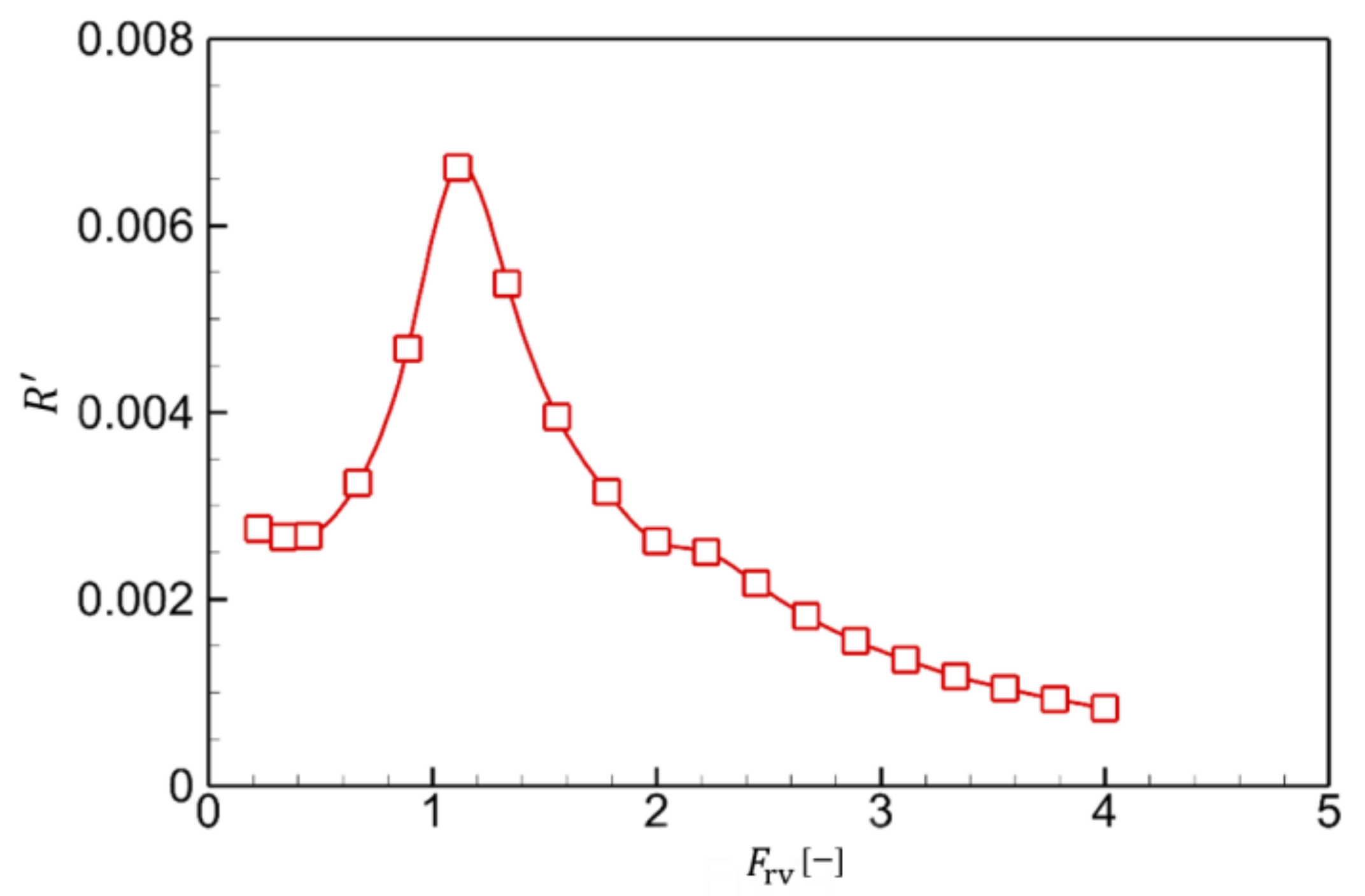
3.1.4. Calculation Result of Direct Navigation Resistance

The direct navigation resistance is calculated, and the Fourier coefficient of the captain is 0.1, 0.15, 0.2, 0.3, 0.4, 0.5, 0.6, 0.7, 0.8, 0.9, 1, 1.1, 1.2, 1.3, 1.4, 1.5, 1.6, 1.7, and 1.8, a total of 19 speeds. The calculation results of the drag are shown in Figure 4. In the figure, the abscissa is the volume Fourier coefficient $F_{\mathrm{rv}}=u/\sqrt{g\nabla }$, and the ordinate is the dimensionless drag $R^{\prime }=R/\left(0.5\rho u^2{L}_{pp}^3\right)$.

As can be seen from the figure, the drag coefficient increases first and then decreases with the increase of the volume Fourier coefficient. When the volume Fourier coefficient is 1, the drag coefficient reaches its maximum value. Figure 5 gives the ripple around the hull at different speeds. As the ship speed increases, the amplitude of the wave is larger, and the wavelength of the wave is longer.

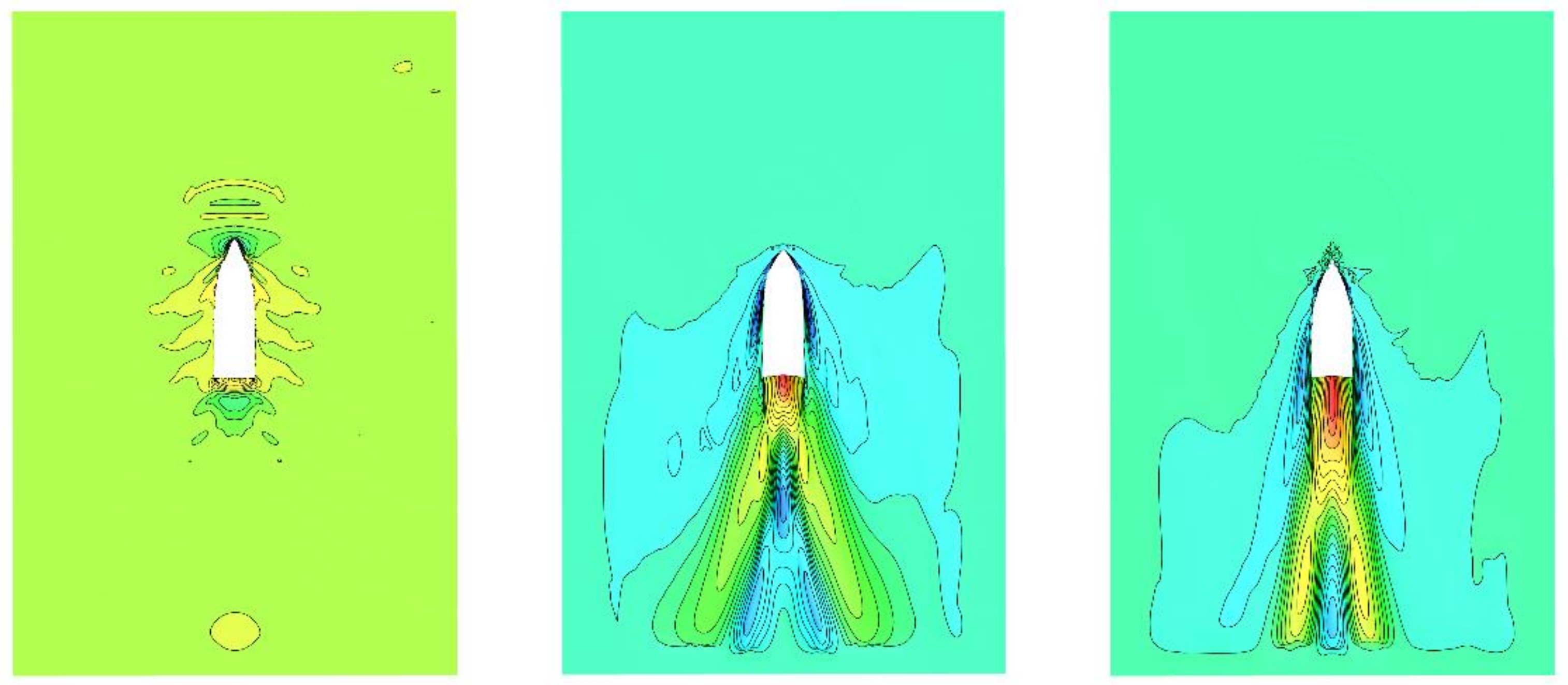
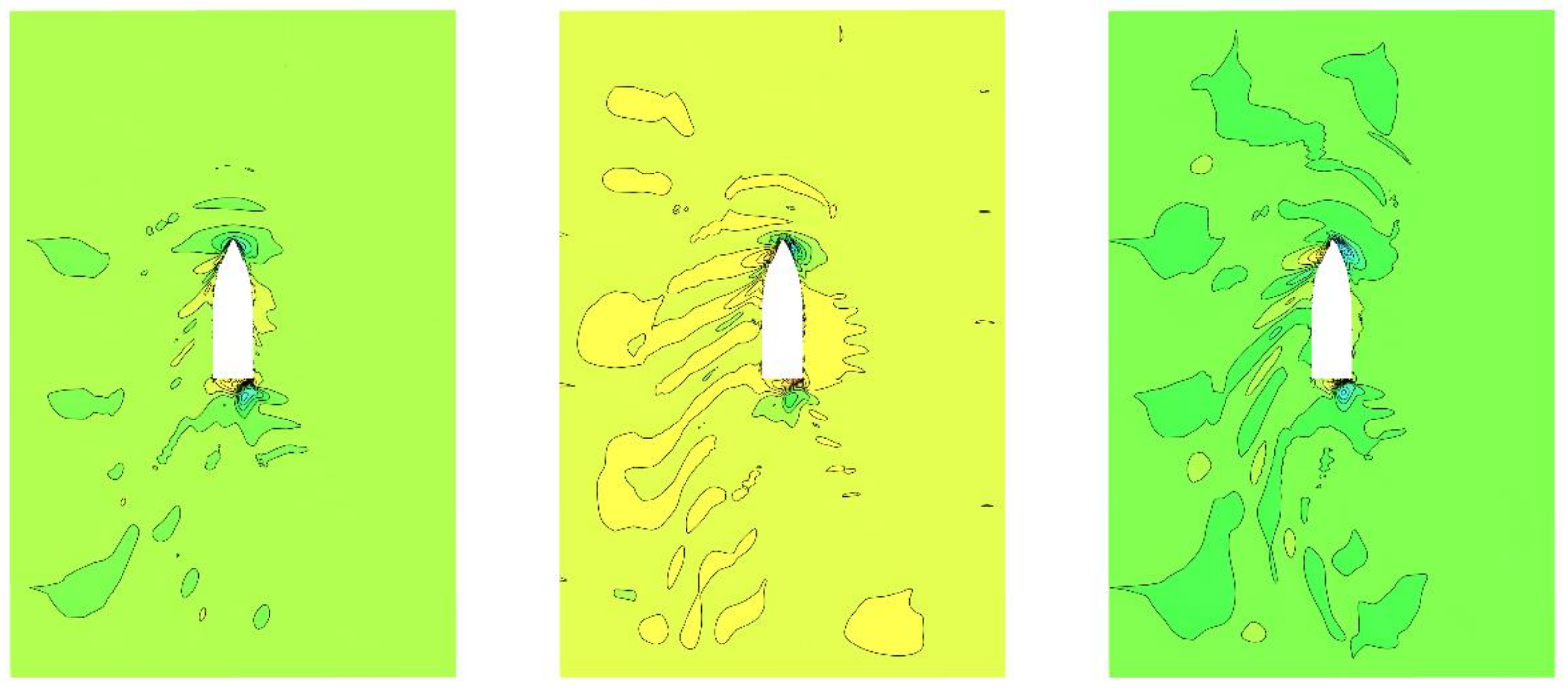
3.1.5. Coupled Hydrodynamics of Oblique Motion and Circling Motion

The coupled hydrodynamics of oblique motion and circling motion of the USV are calculated. The ship’s length Fourier coefficient is 0.2, the drift angles are 0 degrees, ±10 degrees, and ±20 degrees, and the dimensionless steering angular speeds are 0, ±0.4, and ±0.8. Figure 6 shows the ripple of the coupled motion. It can be seen that the variation tendency of the ripple around the hull is reasonable.

3.1.6. Hydrodynamic Derivative

The hydrodynamic derivative can be calculated using regression analysis based on the above calculation, and the hydrodynamic result obtained is shown in

Table 2. Hydrodynamic derivatives.

Hydrodynamic Derivative	Calculated Value
$X_0^{\prime }$	−0.0026
$X_u^{\prime }$	−0.000700
$X_{uu}^{\prime }$	0.002500
$X_{uuu}^{\prime }$	−0.001800
$X_{vv}^{\prime }$	0.002744
$X_{rr}^{\prime }$	−0.002807
$X_{vr}^{\prime }$	0.01247
$Y_v^{\prime }$	−0.01471
$Y_{vvv}^{\prime }$	0.112200
$N_v^{\prime }$	−0.006399
$N_{vvv}^{\prime }$	−0.006952
$Y_r^{\prime }$	0.003013
$Y_{rrr}^{\prime }$	−0.000467
$N_r^{\prime }$	−0.001708
$N_{rrr}^{\prime }$	−0.000261
$Y_{vvr}^{\prime }$	−0.005687
$Y_{vrr}^{\prime }$	−0.013020
$N_{vvr}^{\prime }$	−0.015600
$N_{vrr}^{\prime }$	−0.001047

.

The derivative of acceleration (additional mass) are determined empirically. The acceleration derivative values are: $X_{\dot{u}}^{\prime }=-0.000238$, $Y_{\dot{v}}^{\prime }=-0.007049$, $N_{\dot{v}}^{\prime }=-0.000283$, $Y_{\dot{r}}^{\prime }=-0.000777$, $N_{\dot{r}}^{\prime }=-0.000419$.

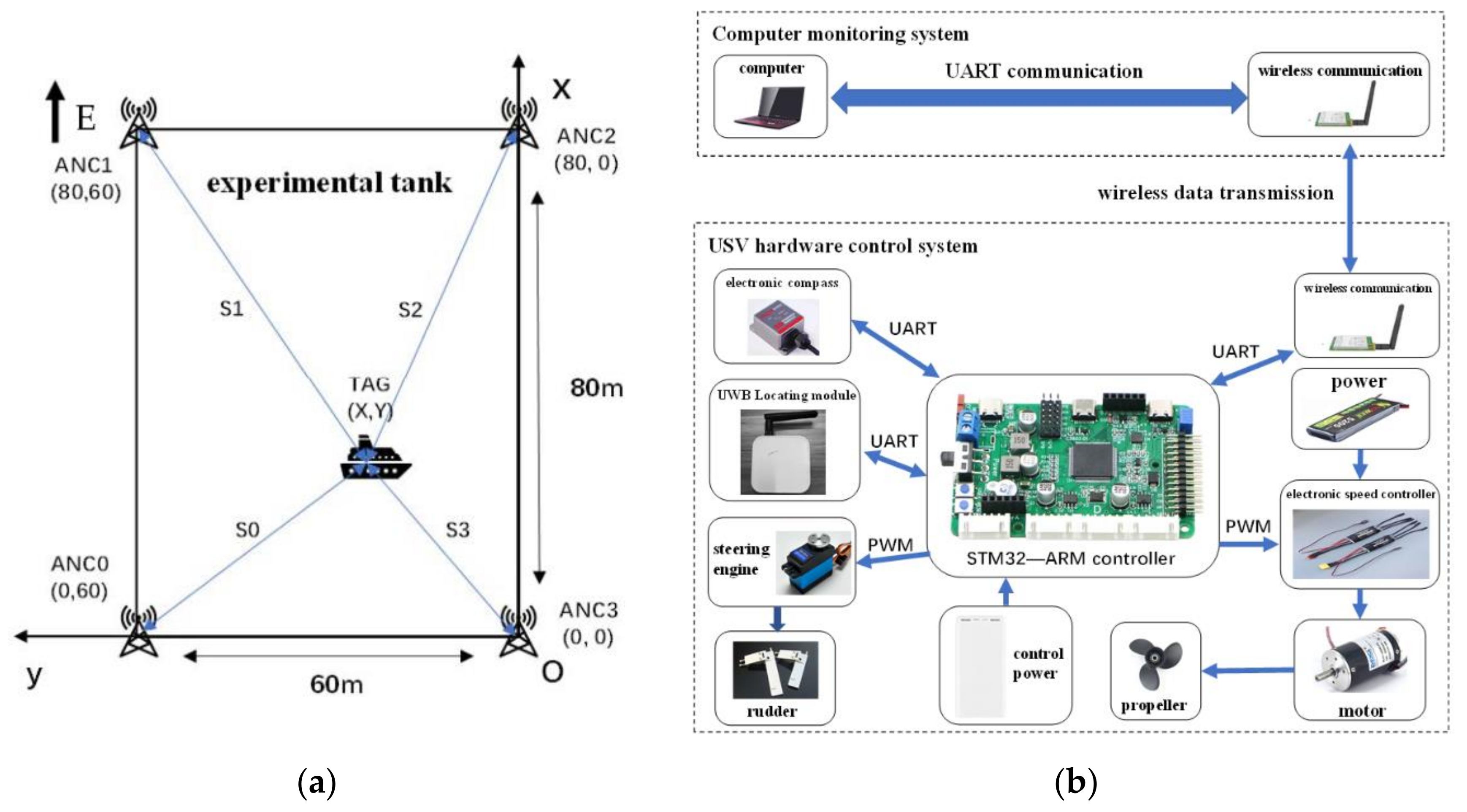
3.2. Test Platform Construction

In order to verify whether the 3-DOF MMG model can accurately describe the motion of a real ship, a USV maneuverability test platform was built. The remote control platform was developed using QT software and is used to send control instructions and receive test data from the USV. The ship is equipped with an electronic compass, Ultra Wide Band (UWB) positioning kit, inertial navigation kit, etc., to collect the current state of the ship’s movement in real time. The USV communicates with the shoreside control platform using the E32 wireless module.

The size of the experimental tank is 60 m × 80 m, the test coordinate system was established as shown in Figure 7a, and the lower right corner of the tank was taken as the origin. Four UWB base stations are placed at the four corners of the tank, covering the range of the test; USV coordinates were calculated using the distance, S0, S1, S2 and S3, from the USV to the four base stations, according to the trilateration measurement method [28]. Using four UWB instead of three UWB could effectively improve positioning accuracy.

The hardware and data transmission system are shown in Figure 7b. On the USV, the STM32 MCU controls the steering gear angle and motor speed by adjusting the PWM output duty ratio. The electronic compass and the UWB positioning module collect the real-time heading angle and the distance between the USV and the four base stations and then transmit the collected data to STM32 using serial port communication (UART). After sorting the data in a specific sequence, STM32 gives the data to the wireless serial port in UART mode. The wireless serial port transmits data to the remote control platform at a transmission rate of 9600 baud and an air data transmission rate of 2400 bit. On the remote control platform, the computer analyzes and stores the received data, calculates the motor speed and the rudder angle at the next moment according to the ship control requirements, and then sends the command back to the STM32 on the USV.

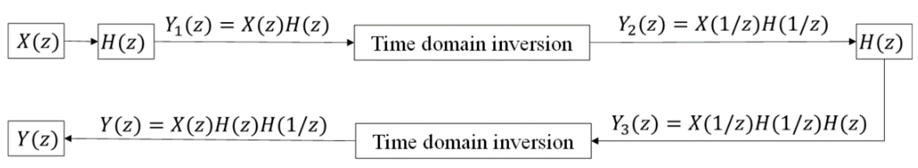
3.3. Test Data Processing

Compared with the simulation data, errors and high-frequency disturbances would exist in the data obtained from the experiment, making the comparison between the simulation data on the MMG model and the experimental data difficult [29]. The errors of the real USV test come mainly from the following aspects: the equipment errors from the angular transducer, locator device, and other sensors, the loss of data in the UWB positioning system caused by environmental interference such as scatterers and ferromagnetic interference, and the imponderable time delay caused by the loss of signal when wireless signals pass through obstacles. To overcome the error caused by the above reasons and reduce the influence of random noise interference, it is necessary to process the test data and eliminate the abnormal data and subsequently perform the smoothing, filtering, and interpolating work on the preprocessed data. In this paper, the Radial Reach Filter (RRF) is used for data processing, and its filtering principle is shown in Figure 8 [30]. First, the signal sequence is passed forward through the filter for filtering to complete the output of the first filtered signal, and then the output signal sequence is reversed on the time axis. Then, the second filtering is carried out through the filter again to complete the output of the second filtering signal, and then the output signal is flipped in the time domain, obtaining the zero phase shift filtering signal with zero phase characteristics.

z represents the frequency domain, that is $z=e^{jw}$, and the process can be expressed as the following formula:

$$\left.\begin{array}{c}{Y}_1\left(e^{jw}\right)=X\left(e^{jw}\right)H\left(e^{jw}\right) \\ Y_2\left(e^{jw}\right)=e^{-jw\left(N-1\right)}{Y}_1\left(e^{-jw}\right) \\ Y_3\left(e^{jw}\right)=Y_2\left(e^{jw}\right)H\left(e^{jw}\right) \\ Y\left(e^{jw}\right)=e^{-jw\left(N-1\right)}{Y}_3\left(e^{-jw}\right) \end{array}\right\}$$

(7)

where $X\left(e^{jw}\right)$ is the input; $Y\left(e^{jw}\right)$ is the output; $H\left(e^{jw}\right)$ is the impulse response sequence; and $Y_i\left(i=1,2,3\right)$ is the intermediate response.

The RRF can display the data trend accurately, but it requires time-reversal processing of the signal sequence, which is impossible for real-time data processing since time cannot travel backward, but it is suitable for offline data processing. Therefore, in this study, the test data were completely collected and filtered, and then compared with the simulation test.

Figure 9 gives the comparison results of the position $\left(x,y\right)$ and the resultant velocity $U$ of the 35° rotation test processed using the RRF, SG filter [31], and Cubic filter [32], respectively. The figure shows that the data processed using the SG smoothing filter is close to the original motion trajectory, but it is sensitive to large-value interference. The trajectory data processed using Cubic interpolation is smoother than the original data, but it has a poor smoothing effect on the velocity. The result of the RRF is smoother and closer to the real value; the high-frequency noise is also effectively reduced. So, the RRF is used for subsequent data procession of the angular velocity, speed, and other data information in the test.

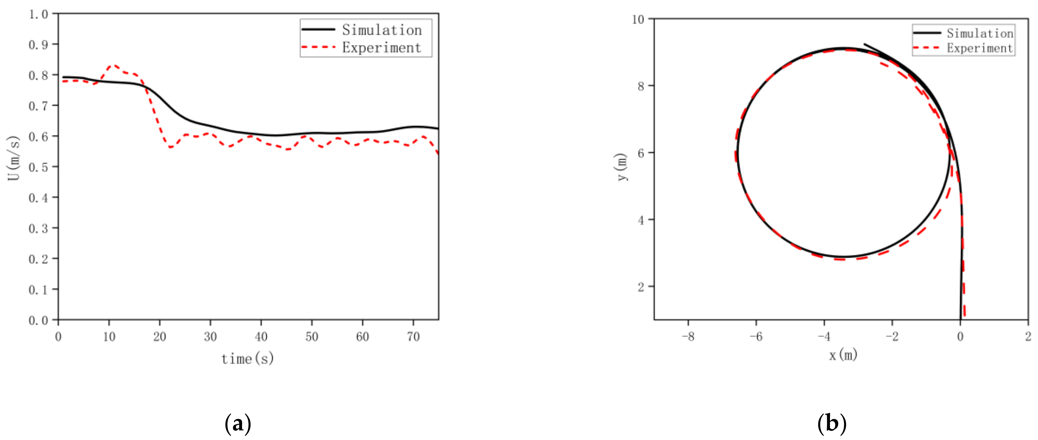
3.4. Validity Verification of Simulation Samples

In this section, the 35° rotation test is discussed, and the test platform data are compared and analyzed with the simulation data to demonstrate the collaboration effectiveness of the test and simulation in obtaining samples.

(1)

Test platform data acquisition

The USV first performed a straight-line navigation after the speed of the USV became stable, and the shoreside upper computer sent a turning command to the USV for performing the 35° turning maneuvering. The experiment ended when the USV heading had changed by 540°.

(2)

Simulation data acquisition

The hydrodynamic derivative of the ship calculated using CFD was substituted into the MMG model for maneuverability simulation. With a simulation step size of 0.01 s, the numerical simulation of the 35° turning maneuvering was carried out, and the simulation ended when the heading had changed 540° as well. The data obtained from the simulation are equidistantly extracted with a ratio of 1% to form the sample data, which contained 80 samples. The coordinates and speed comparison of simulation and experiment of the 35° rotation are given in Figure 10.

As can be seen in Figure 10, in the steady state rotary diameter, the difference in tactical diameter, longitudinal and transverse distance, and other characteristic parameters between the test and simulation is less than 15% in both straight-line navigation and turning conditions, indicating that the 3-DOF MMG model can accurately describe the motion state of the USV. Therefore, on the one hand, data generalization can be carried out using simulation to form a large number of test samples for black-box model training; on the other hand, the black-box model trained using simulation data can be verified with experiments.

4. The SSA-WLS-SVM Algorithm

The black-box model is commonly used in neural network and fuzzy control models. The core algorithm of the neural network is based on the principle of empirical risk minimization, which has a problem of “over fitting” in practice. Vapnik [33] first introduced support vector machines (SVMs) in 1995 to solve the problem of pattern recognition. The standard support vector machine (SVM) uses the structural risk minimization principle to overcome this shortcoming and has the advantages of robustness and sparsity. Robustness means that its solution is stable, and sparsity means that the training samples are all effective support vectors that contribute to the objective function. However, the parameter adjustment on the SVM algorithm is relatively difficult, and the calculation amount brought by inequality is large. The least squares support vector machine (LSSVM) is an extension of SVM, which improves the solving speed of the black-box model but loses the advantages of the robustness and sparsity of the SVM. In this paper, a black-box model with weighted least squares support vector machine (WLS-SVM) based on the Sparrow search algorithm (SSA) is proposed to perform regression training on USV motion samples.

The sample set $\mathrm{S}=\left\{\left({\mathit{x}}_{\mathit{i}},{\mathit{y}}_{\mathit{i}}\right),\left({\mathit{x}}_{\mathit{i}},{\mathit{y}}_{\mathit{i}}\right)\in {\mathit{R}}_{\mathit{N}},i=1,2,\cdots ,N\right\}$, where ${\mathit{R}}_{\mathit{N}}$ is the original data space. The sample is mapped from the original low-dimensional space ${\mathit{R}}_{\mathit{N}}$ to the high-dimensional feature space ${\mathit{\psi }}_{\mathit{N}}$ using the nonlinear mapping function $\phi \left(x\right)$, and the low-dimensional nonlinear problem is transformed into a high-dimensional linear problem simplifying the complex nonlinear relationship between ${\mathit{x}}_{\mathit{i}}$ and ${\mathit{y}}_{\mathit{i}}$. The set of samples corresponding to ${\mathit{\psi }}_{\mathit{N}}$ space is represented as $\tilde{\mathrm{S}}=\left\{\left[\phi \left({\mathit{x}}_{\mathit{i}}\right),{\mathit{y}}_{\mathit{i}}\right],\left({\mathit{x}}_{\mathit{i}},{\mathit{y}}_{\mathit{i}}\right)\in {\mathit{R}}_{\mathit{N}},i=1,2,\cdots ,N\right\}$. Thus, the optimal decision function can be constructed in the high-dimensional space, which is also called the “hyperplane” [34]:

$$\mathit{y}\left(\mathit{x}\right)={\mathit{\omega }}^{\mathit{T}}\phi \left(\mathit{x}\right)+\mathit{b}$$

(8)

where $\mathit{\omega }$ is the normal vector that determines the direction of the hyperplane; and $\mathit{b}$ is the displacement term that determines the distance between the hyperplane and the origin.

The optimization equations of the algorithm are as follows:

$$\begin{array}{c}\underset{\omega ,b}{\min }\mathrm{J}\left(\mathit{\omega }\right)=\frac{1}{2}║\mathit{\omega }{║}^2+\mathrm{C}{\displaystyle \sum _{i=1}^N}\left({\xi }_i+{\xi }_i^{\ast }\right)\\ s.t. \left\{\begin{array}{c}{\mathit{y}}_{\mathit{i}}-\left[{\mathit{\omega }}^T\phi \left({\mathit{x}}_{\mathit{i}}\right)+\mathit{b}\right]\le \epsilon +{\xi }_i\\ {\mathit{\omega }}^T\phi \left({\mathit{x}}_{\mathit{i}}\right)+\mathit{b}-{\mathit{y}}_{\mathit{i}}\le \epsilon +{\xi }_i^{\ast }\\ {\xi }_i,{\xi }_i^{\ast }\ge 0\end{array}\right.\end{array}$$

(9)

where $\mathrm{C}$ is the penalty parameter, which is a constant that needs to be determined; and ${\xi }_i$ and ${\xi }_i^{\ast }$ is the interval relaxation factor introduced to ensure that the objective function has a solution under the constraint. $\epsilon$ is an insensitive loss factor and represents the allowable training loss.

The SVM has been widely used by scholars because of its promotion in generalization ability and reduction in curse of dimensionality due to the introduction of the kernel function. However, its generalization performance mainly depends on the selection of the kernel function and the design of the penalty parameters and insensitive loss factors. To improve the rapidity of the SVM algorithm and reduce the uncertainty of parameter adjustment, LS-SVM [35] transforms the inequality conditions in Equation (9) into equality constraints, which improves the calculation speed while reducing the optimization parameter $\epsilon$. The multilayer neural network (MLP) training procedure is also used, introducing the sum of error squares (SSE) into the optimization problem and adding the term $\frac{1}{2}\mathrm{C}\sum _{\mathrm{i}=1}^{\mathrm{N}}{e}_i^2$, to transform the optimization problem into:

$$\begin{array}{c}\underset{\mathsf{\omega },b,e_i}{\min }\mathrm{J}\left(\mathsf{\omega }\right)=\frac{1}{2}║\mathit{\omega }{║}^2+\frac{1}{2}\mathrm{C}{\displaystyle \sum _{\mathrm{i}=1}^{\mathrm{N}}}{\mathit{e}}_{\mathit{i}}{}^2\\ s.t. {\mathit{y}}_{\mathit{i}}-\left[{\mathsf{\omega }}^T\phi \left({\mathit{x}}_{\mathit{i}}\right)+\mathit{b}\right]={\mathit{e}}_{\mathit{i}},i=1,2,\cdots ,N\end{array}$$

(10)

where ${\mathit{e}}_{\mathit{i}}$ is the error variable, numerically equal to the difference between the output data ${\mathit{y}}_{\mathit{i}}$ and the optimal decision function $\mathit{y}\left(\mathit{x}\right)$.

Equation (10) is an equation quadratic programming (QP) problem, and its corresponding Lagrange function is:

$$\mathcal{L}\left(\mathit{w},\mathit{b},{\mathit{e}}_{\mathit{i}},{\alpha }_i\right)=\frac{1}{2}║\mathit{\omega }{║}^2+\frac{1}{2}\mathrm{C}{\displaystyle \sum }_{\mathrm{i}=1}^{\mathrm{N}}{\mathit{e}}_{\mathit{i}}{}^2-{\displaystyle \sum }_{\mathrm{i}=1}^{\mathrm{N}}{\alpha }_i\left({\mathbf{w}}^T\phi \left({\mathit{x}}_{\mathit{i}}\right)+\mathit{b}+{\mathit{e}}_{\mathit{i}}-{\mathit{y}}_{\mathit{i}}\right)$$

(11)

where ${\alpha }_i$ is the Lagrange multiplier, $i=1,2,\cdots ,N$.

Although the LS-SVM has been widely used because of its simple characteristic, its solution does not achieve the characteristic of sparsity due to the simplification of constraints. In other words, not all samples involved in training are support vectors, leading to inaccurate output when the basic assumption, that the error variable ${\mathit{e}}_{\mathit{i}}$ is the Gaussian distribution, is not valid.

In WLS-SVM [36,37], the weighting coefficient $v_i\left(i=1,2,\cdots ,N\right)$ is adopted to grant the weight of the error variable ${\mathit{e}}_{\mathit{i}}$ in LS-SVM and converts the optimization Equation (10) into:

$$\begin{array}{c}\min \left(\frac{1}{2}║{\mathit{\omega }}^{\ast }{║}^2+\frac{1}{2}\mathrm{C}{\displaystyle \sum _{\mathrm{i}=1}^{\mathrm{N}}}{v}_i{\mathit{e}}_{\mathit{i}}^{\ast }{}^2\right)\\ s.t.{\mathit{y}}_{\mathit{i}}-\left[{\mathit{\omega }}^{\ast \mathit{T}}\phi \left({\mathit{x}}_{\mathit{i}}\right)+{\mathit{b}}^{\ast }\right]={\mathit{e}}_{\mathit{i}}^{\ast },i=1,2,\cdots ,N\end{array}$$

(12)

The Lagrange function corresponding to Equation (9) is:

$$\mathcal{L}\left({\mathit{\omega }}^{\ast },{\mathit{b}}^{\ast },{\mathit{e}}_{\mathit{i}}^{\ast },{\alpha }_i^{\ast }\right)=\frac{1}{2}║{\mathit{\omega }}^{\ast }{║}^2+\frac{1}{2}\mathrm{C}{\displaystyle \sum }_{\mathrm{i}=1}^{\mathrm{N}}{v}_i{\mathit{e}}_{\mathit{i}}^{\ast }{}^2-{\displaystyle \sum }_{\mathrm{i}=1}^{\mathrm{N}}{\alpha }_i^{\ast }\left({\mathit{\omega }}^{\ast \mathit{T}}\phi \left({\mathit{x}}_{\mathit{i}}\right)+{\mathit{b}}^{\ast }+{\mathit{e}}_{\mathit{i}}^{\ast }-{\mathit{y}}_{\mathit{i}}\right)$$

(13)

The symbol * in Equations (12) and (13) represents the variable after weighting. ${\alpha }_i^{\ast }$ is the weighted Lagrange multiplier; ${\mathit{b}}^{\ast }$ is the weighted displacement term; and ${\mathit{e}}_{\mathit{i}}^{\ast }$ is the weighted error variable, $i=1,2,\cdots ,N$.

Equation (13) is solved according to the Karush–Kuhn–Tucker (KKT) condition,

$$\left\{\begin{array}{l}\frac{\partial \mathcal{L}}{\partial {\mathsf{\omega }}^{\ast }}=0\Rightarrow {\mathsf{\omega }}^{\ast }={\displaystyle {\displaystyle \sum }_{\mathrm{i}=1}^{\mathrm{N}}}{\alpha }_i^{\ast }\mathsf{\phi }\left({\mathit{x}}_{\mathit{i}}\right)\\ \frac{\partial \mathcal{L}}{\partial {\mathit{b}}^{\ast }}=0\Rightarrow {\displaystyle {\displaystyle \sum }_{\mathrm{i}=1}^{\mathrm{N}}}{\alpha }_i^{\ast }=0\\ \frac{\partial \mathcal{L}}{\partial {\mathit{e}}_{\mathit{i}}^{\ast }}=0\Rightarrow {\alpha }_i^{\ast }=\mathrm{C}{v}_i{\mathit{e}}_{\mathit{i}}^{\ast }\\ \frac{\partial \mathcal{L}}{\partial {\alpha }_i^{\ast }}=0\Rightarrow {\mathit{\omega }}^{\ast \mathit{T}}\mathsf{\phi }\left({\mathit{x}}_{\mathit{i}}\right)+{\mathit{b}}^{\ast }+{\mathit{e}}_{\mathit{i}}^{\ast }-{\mathit{y}}_{\mathit{i}}=0\end{array}\right.$$

(14)

${\mathsf{\omega }}^{\ast }$ and ${\mathit{e}}_{\mathit{i}}^{\ast }$ were eliminated to form Equation (15):

$$\left[\begin{array}{cc}\mathit{0}& {\mathit{E}}^{\mathit{T}}\\ \mathit{E}& \mathit{A}\end{array}\right]\left[\begin{array}{c}{\mathit{b}}^{\ast }\\ {\mathit{\alpha }}^{\ast }\end{array}\right]=\left[\begin{array}{c}\mathit{0}\\ \mathit{Y}\end{array}\right]$$

(15)

In order to simplify the calculation of the inner product in the high-dimensional space, this paper introduces the kernel function ${\mathit{K}}_{\mathit{i}\mathit{j}}=K{\left({\mathit{x}}_{\mathit{i}},{\mathit{x}}_{\mathit{j}}\right)}_{i,j=1,2,\cdots ,N}=\mathsf{\phi }{\left({\mathit{x}}_{\mathit{i}}\right)}^T\mathsf{\phi }\left({\mathit{x}}_{\mathit{j}}\right)$ to describe the nonlinear mapping $\mathsf{\phi }\left(\mathrm{x}\right)$ of Equation (12), the inner product of ${\mathit{x}}_{\mathit{i}}$ and ${\mathit{x}}_{\mathit{j}}$ in the high-dimensional characteristic space ${\mathit{\psi }}_{\mathit{N}}$ is equal to the result calculated by $\mathit{K}\left(\cdot ,\cdot \right)$ for the original low-dimensional space ${\mathit{R}}_{\mathit{N}}$ [26]. Where ${\mathit{\alpha }}^{\ast }$ is the weighted Lagrange multiplier submatrix, ${\mathit{\alpha }}^{\ast }=\left[{\alpha }_1^{\ast };\cdots ;{\alpha }_N^{\ast }\right]$; $\mathit{E}={\left[1;\cdots ;1\right]}^T,\mathit{E}\in {\mathit{R}}_{N\times 1}$; $\mathit{Y}=\left[{\mathit{y}}_{\mathbf{1}};\cdots ;{\mathit{y}}_{\mathit{N}}\right],\mathit{Y}\in {\mathit{R}}_{N\times 1}$; $\mathit{\Omega }=\left\{{\mathit{K}}_{\mathit{i}\mathit{j}}=\mathit{K}\left({\mathit{x}}_{\mathit{i}},{\mathit{x}}_{\mathit{j}}\right)\right\},\mathit{\Omega }\in {\mathit{R}}_{N\times N}$; and $\mathit{A}=\mathit{\Omega }+diag\left\{\frac{1}{C{v}_1},\dots ,\frac{1}{C{v}_N}\right\}$.

According to Equation (14), the following results can be obtained:

$$\begin{array}{c}{\mathit{b}}^{\ast }=\frac{{\mathit{E}}^{\mathit{T}}{\mathit{A}}^{-\mathbf{1}}\mathit{Y}}{{\mathit{E}}^{\mathit{T}}{\mathit{A}}^{-\mathbf{1}}\mathit{E}}\\ {\mathit{\alpha }}^{\ast }={\mathit{A}}^{-\mathbf{1}}\left(\mathit{Y}-\mathit{E}{\mathit{b}}^{\ast }\right)\end{array}$$

(16)

Equation (14) was transformed to obtain the final WLS-SVM regression modeling model. Equation (8) was combined to form Equation (17).

$$\mathit{y}\left(\mathit{x}\right)={\displaystyle \sum }_{i=1}^N{a}_i^{\ast }\mathit{K}\left(\mathit{x},{\mathit{x}}_{\mathit{i}}\right)+{\mathit{b}}^{\ast }={\mathit{\omega }}^{\mathbf{T}}\phi \left(\mathit{x}\right)+\mathit{b}$$

(17)

The weighting coefficient is determined according to the error variable ${\mathit{e}}_{\mathit{i}}$ of the unweighted LS-SVM in Equation (10):

$$v_i=-\left\{\begin{array}{cc}1,& \left|\frac{{\mathit{e}}_{\mathit{i}}}{\widehat{S}}\right|<{\mathsf{\tau }}_1\\ \frac{{\mathsf{\tau }}_2-\left|\frac{{\mathit{e}}_{\mathit{i}}}{\widehat{S}}\right|}{{\mathsf{\tau }}_2-{\mathsf{\tau }}_1},& {\mathsf{\tau }}_1\le \left|\frac{{\mathit{e}}_{\mathit{i}}}{\widehat{S}}\right|\le {\mathsf{\tau }}_2\\ {10}^{-4},& else\end{array}\right.$$

(18)

In the formula, ${\mathsf{\tau }}_1$ and ${\mathsf{\tau }}_2$ are generally taken as ${\mathsf{\tau }}_1=2.5,{\mathsf{\tau }}_2=3$ [38]. $\widehat{S}$ is the robust estimate standard variance of error variable ${\mathit{e}}_{\mathit{i}}$ in LS–SVM:

$$\widehat{S}=1.483 \mathrm{MAD}\left({\mathit{e}}_{\mathit{i}}\right)$$

(19)

where MAD stands for the absolute median difference.

The WLS-SVM in Equation (18) ignores the assumption that the error variable ${\mathit{e}}_{\mathit{i}}$ in LS-SVM should follow the Gaussian distribution; the two weights, ${\mathsf{\tau }}_1$ and ${\mathsf{\tau }}_2$, can correct outliers or non-Gaussian error distributions of the outputs, so as to obtain robust estimates when the distribution is abnormal. On the basis of the optimization, stable and robust estimation output and be obtained.

In this paper, the Radial Basis Function (RBF) is used to conduct WLS-SVM training:

$${\mathit{K}}_{\mathit{i}\mathit{j}}=K\left({\mathit{x}}_{\mathit{i}},{\mathit{x}}_{\mathit{j}}\right)=\exp \left(-\frac{║{\mathit{x}}_{\mathit{i}}-{\mathit{x}}_{\mathit{j}}║{}^2}{K}\right)$$

(20)

where K is the parameter of the kernel function that represents the influence of a single training sample on the regressor.

The sparrow search algorithm (SSA), proposed by Xue Jiankai [39], simulates the foraging and antipredation behaviors of sparrows for optimization. On the basis of the position iteration formula of three kinds of sparrow particle (discovering, following, and detective particle), the fitness value of sparrow is calculated using the fitness function to realize the role and position transformation among sparrow particles. Finally, the position of the sparrow particle with the highest fitness value is obtained. The SSA effectively avoids the local optimum problem by constructing a fitness function to evaluate moving particles.

The dimension of each sparrow was set as $D=2$, which was equal to the number of parameters to be optimized. The number of sparrows in the population is $n=20$. The randomly initialized sparrow population matrix $\mathit{X}\left(\mathit{X}\in {\mathit{R}}_{20\times 2}\right)$ can be expressed as:

$$\mathit{X}=\left[\begin{array}{c}\begin{array}{cc}{C}_{11}& K_{12}\end{array}\\ \begin{array}{cc}{C}_{21}& K_{22}\end{array}\\ \begin{array}{cc}⋮& ⋮\end{array}\\ \begin{array}{cc}{C}_{20,1}& K_{20,2}\end{array}\end{array}\right]$$

(21)

Then, the position of the $q_{th}$ individual sparrow in the space is $X_q=\left[C_{q1},K_{q2}\right],q=1,2,\cdots ,20$.

Let $g\left(X_q\right)$ be the fitness value of the sparrow, equal to the root mean square error (RMSE) between the predicted data and the real data:

$$RMSE=\sqrt{\frac{1}{N}{\displaystyle \sum }_{i=1}^N{\left({\widehat{\mathit{y}}}_{\mathit{i}}-{\mathit{y}}_{\mathit{i}}\right)}^2}$$

(22)

among them, ${\widehat{\mathit{y}}}_{\mathit{i}}$ stands for the forecast output based on the $i_{th}$ input sample vector ${\mathit{x}}_{\mathit{i}}$, and ${\mathit{y}}_{\mathit{i}}$ for the corresponding actual output.

The population fitness matrix is expressed by Equation (20):

$${\mathit{G}}_{\mathit{x}}=\left[\begin{array}{c}g\left(X_1\right)\\ \begin{array}{c}g\left(X_2\right)\\ ⋮\\ g\left(X_{20}\right)\end{array}\end{array}\right]=\left[\begin{array}{c}g\left(\left[C_{11},K_{12}\right]\right)\\ \begin{array}{c}g\left(\left[C_{21},K_{22}\right]\right)\\ ⋮\\ g\left(\left[C_{20,1},K_{20,2}\right]\right)\end{array}\end{array}\right]$$

(23)

In the group foraging process, the responsibility of the discovering particles is to look for food and provide foraging range for the population. The following particles are to forage together with the discoverer particles later after the food is located by discoverer particles, and the detective particles are to raise the alarm when danger is discovered in the foraging process. The discoverer particle constantly updates its location to search foraging areas and obtain the food that the population needs. After the food is located, the following particles follow the location and obtain a higher fitness. When threatened by a predator, the detective particles raise the alarm to the population for performing anti-predator behavior.

The position of the discovering particle is updated on Equation (24):

$$X_{q,d}^{iter+1}\left\{\begin{array}{cc}{X}_{q,d}^{iter}·\exp \left(-\frac{i}{\lambda ·ite{r}_{max}}\right)& if R_2<ST\\ X_{q,d}^{iter}+Q·L& if R_2\ge ST\end{array}\right.$$

(24)

where $iter$ is the time of current iterations, $ite{r}_{max}$ represents the maximum time of iterations, which is set to 128, $\lambda$ is a random number in $\left(0,1\right], R_2\in \left(0,1\right)$ represents the alert value, $ST\in \left(0.5,1\right)$ represents the security threshold, Q is the matrix of random numbers complying with the normal distribution, and $L\in {\mathit{R}}_{1\times 2}$, represents a matrix in which elements are all 1. $R_2<ST$ means no predator was found and the discovering particles can perform a search in the global scope. $R_2\ge ST$ represents that the detective particles have located the predator.

The position of the following particle is updated on Equation (25):

$$X_{q,d}^{iter+1}\left\{\begin{array}{cc}Q·\exp \left(\frac{X_{worst}-X_{q,d}^{iter}}{q^2}\right)& if q>\frac{n}{2}\\ X_p^{iter}+\left|X_{q,d}^{iter}-X_p^{iter}\right|·A^{+}·L& else\end{array}\right.$$

(25)

where $A^{+}\in {\mathit{R}}_{1\times 2}$ whose elements are composed of 1 or −1 randomly, $X_p^{iter}$ represents the best position of the current discovering particle, and $X_{worst}$ represents the worst global position of the current discovering particle. $q>n/2$ indicates that the qth following particle does not perform well since it has a low fitness value and needs to forage in other places.

The position of the detective particle is updated on Equation (26):

$$X_{q,d}^{iter+1}\left\{\begin{array}{cc}{X}_{best}^{iter}+\beta ·\left|X_{q,d}^{iter}-X_{best}^{iter}\right|& if f_q>f_g\\ X_{q,d}^{iter}+G·\left(\frac{\left|X_{q,d}^{iter}-X_{worst}^{iter}\right|}{\left(f_q-f_w\right)+\gamma }\right)& if f_q=f_g\end{array}\right.$$

(26)

where $X_{best}^{iter}$ is the global optimal position at the moment; $\beta$ is the parameter controlling the step length, complying with the $N\left(0,1\right)$ distribution, $U\in \left[-1,1\right]$; $f_q$ means the fitness value of the $q_{th}$ sparrow at the moment; $f_g$ is the optimum fitness value of the $q_{th}$ sparrow till now; $f_w$ is the corresponding worst fitness value ever; and $\gamma$ is a constant. $f_q>f_g$ indicates that the sparrow is at the edge of the colony. $f_q=f_g$ represents that the sparrow in the center of the swarm is aware of danger and needs to move close to other sparrows to avoid preying. $G$ is a vector that represents both the direction in which the sparrow moves toward and the parameter that controls the step length.

The structure of the model of SSA-WLS-SVM is shown in Figure 11, and the algorithm steps are summarized as follows:

(1)

The sample set $S=\left\{\left(x_i,y_i\right),\left(x_i,y_i\right)\in {\mathit{R}}_{\mathit{N}},i=1,2,\cdots ,N\right\}$ given by WLS-SVM is taken as the benchmark, the regularization parameter $C$ and kernel parameter $K$ of WLS-SVM were taken as the optimization objects of the SSA algorithm. The sparrow population size, iteration times, and initial safety threshold are determined to initialize the SSA optimization algorithm.

(2)

Initial or subsequent updated values of $C$ and $K$ are taken as optimization parameters of the LS-SVM algorithm, and the LS-SVM Lagrange multiplier ${\alpha }_i$ is weighted to obtain error variables $e_i={\alpha }_i/C$. According to Equation (16), the standard variance $e_i$ is taken to calculate $\widehat{S}$; then, the weighted coefficient $v_i$ is determined based on $e_i$ and $\widehat{S}$, and Equation (13) is solved to obtain the WLS-SVM model corresponding to the $C$ and $K$ values.

(3)

The RMSEs of both the predicted value $\widehat{\mathit{y}}$ from the WLS-SVM model and the actual sample value $\mathit{y}$ are used to calculate the adaptive value of each sparrow.

(4)

Update the position of the sparrow particles based on Equations (21)–(23) to obtain the fitness value of the sparrow population, and save the optimal individual position and global optimal position in the population.

(5)

Check whether the termination conditions have been met or whether the maximum number of update iterations has been reached. If yes, the loop will end and the optimal individual solution, which determines a set of optimal parameters of WLS-SVM, will be returned; otherwise, steps (2)–(4) will continue.

(6)

Take the optimal particle value output using the SSA algorithm as the regularization parameter $C$ and kernel parameter $K$ in WLS-SVM. Step (2) is repeated to calculate the WLS-SVM model corresponding to the optimal regularization parameter $C$ and kernel parameter $K$.

5. Model Training

5.1. Design and Pre-Processing of Datasets

Referring to the research of Professor Zou Zaojian et al. [23], the multi-output ν vector machine is used for the simulation of ship motion, and the random maneuvering test is adopted for training. The resulting trained model is better than the one trained with the test data of 20°/20° zigzag maneuvering. As the effectiveness of the 3-DOF MMG model has been verified in the 35° turning maneuvering test above, the simulation data of the model can be used for black-box model training.

Firstly, the training set was obtained using the 3-DOF MMG model simulation: the hydrodynamic coefficients of the USV calculated using CFD were substituted into the MMG model for the maneuvering simulation. The timestep was 0.01 s, the duration was 300 s, and the initial USV speed was 0.8 m/s. The random maneuvering test with the rudder angle changing in the range of $\delta ϵ\left[-35,35\right]$ in every 8 s was carried out. Dataset No. 1, with 300 samples out of 30,000 samples, was used for training. Based on the theory in Section 2, longitudinal velocity, lateral velocity, steering angular speed, and steering angle are used as input $\mathit{x}$, while longitudinal acceleration, lateral acceleration, and steering angular acceleration are used as output $y$.

To equally consider each parameter in the input vector and output vector, the MaxAbsScaler method is used to normalize the data:

$$\begin{array}{c}{x}_{formal}=x./\max \left(\left|x\right|\right)\\ y_{formal}=y./\max \left(\left|y\right|\right)\end{array}$$

(27)

where $x_{formal}$ is the input after normalization and $y_{formal}$ is the output after normalization.

Following the simulation and preprocessing process described above, a 25° turning maneuvering simulation was performed to form the maneuvering dataset No. 3, and both the random maneuvering dataset No. 2 and the 25° turning dataset No. 3 were used for generalization verification. The uses of the different data sets are shown in the

Table 3. Datasets for training, validation, and testing.

Datasets	Details of Dataset
Training sets	random maneuvering dataset No.1
Test sets	random maneuvering dataset No.2
Generalized set	random maneuvering dataset No.2
	25° turning dataset No.3

.

5.2. Model Training

The proposed SSA-WLS-SVM method was used for parameter optimization and dataset training. In the parameter optimization process, the dimension of the sparrow population was set to 2, the number of sparrows was 20, and the proportion of discovery of the sparrow was 70%. The warning value was 0.6, the maximum number of iterations was 128, the parameter optimization range was set as $C=1e4~1e6$, $K=50~200$. The 10-fold cross validation method was used for the discriminant criterion of parameter optimization. Three groups of optimization parameters were obtained, for $u$, $v$ and $r$, the optimized parameters $\left(C, K\right)$ are $\left(835170.71, 131.17\right)$, $\left(901565.56, 170.06\right)$ and $\left(386631.116, 54.496\right)$, respectively. The 300 input samples were considered as support vectors. The regression model of the SVM with weighted Lagrange multiplier ${\alpha }_i^{\ast }$, weighted displacement term ${\mathit{b}}^{\ast }$ was established.

The trained SVM is used to predict the entire navigation process in the random maneuvering dataset 1, and longitudinal acceleration $\dot{u}$, lateral acceleration $\dot{v}$, steering angular acceleration $\dot{r}$ can be outputted. Subsequently, the longitudinal velocity $u$, lateral velocity $v$, steering angular speed $r$, and USV track can also be obtained. As shown in Figure 12, by comparing the prediction results of SSA-WLS-SVM with the simulation results of the MMG model, it can be concluded that the black-box modeling and prediction method based on SSA-WLS-SVM can accurately predict the ship’s 3-DOF motion.

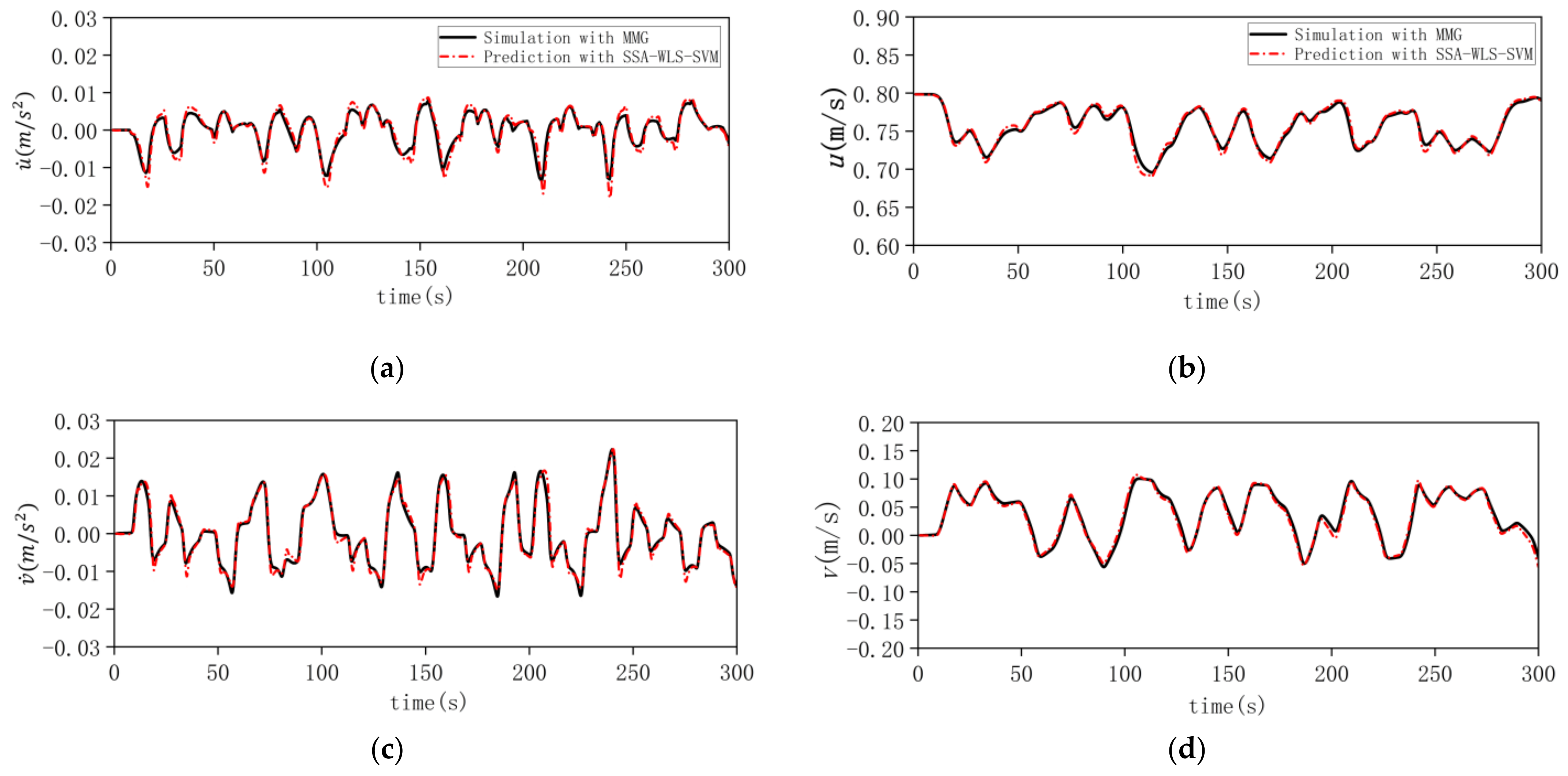
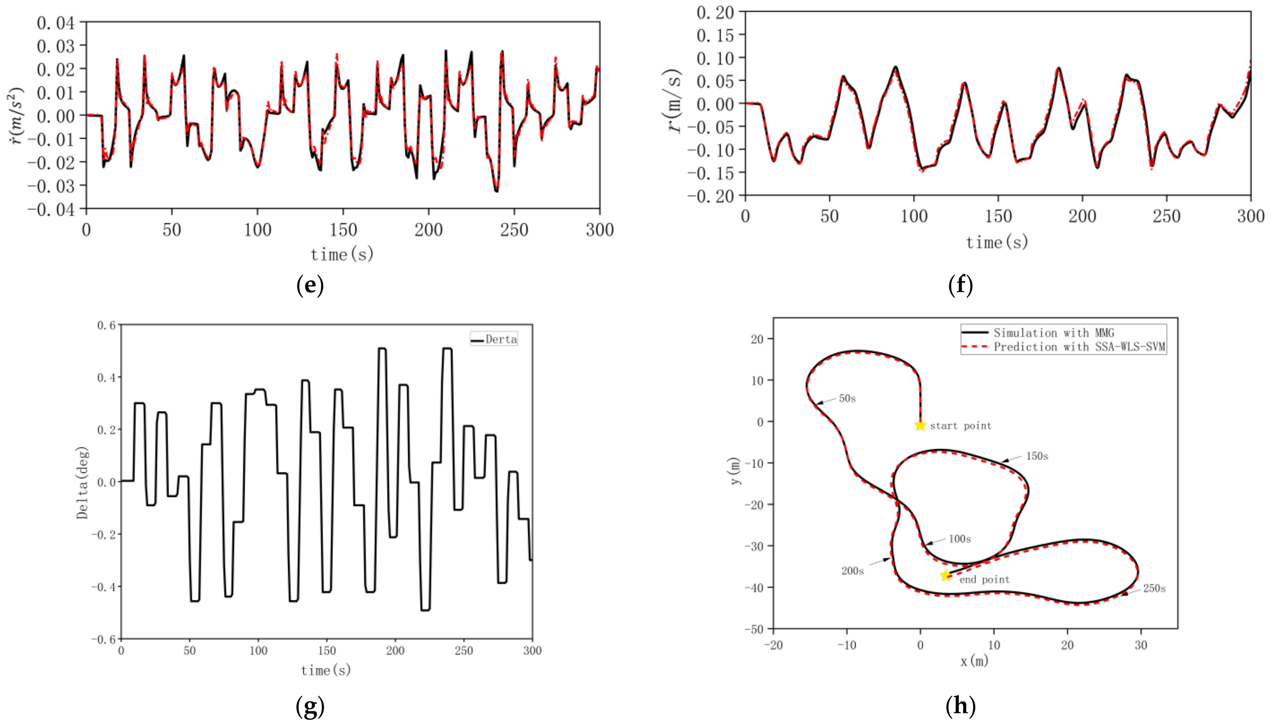
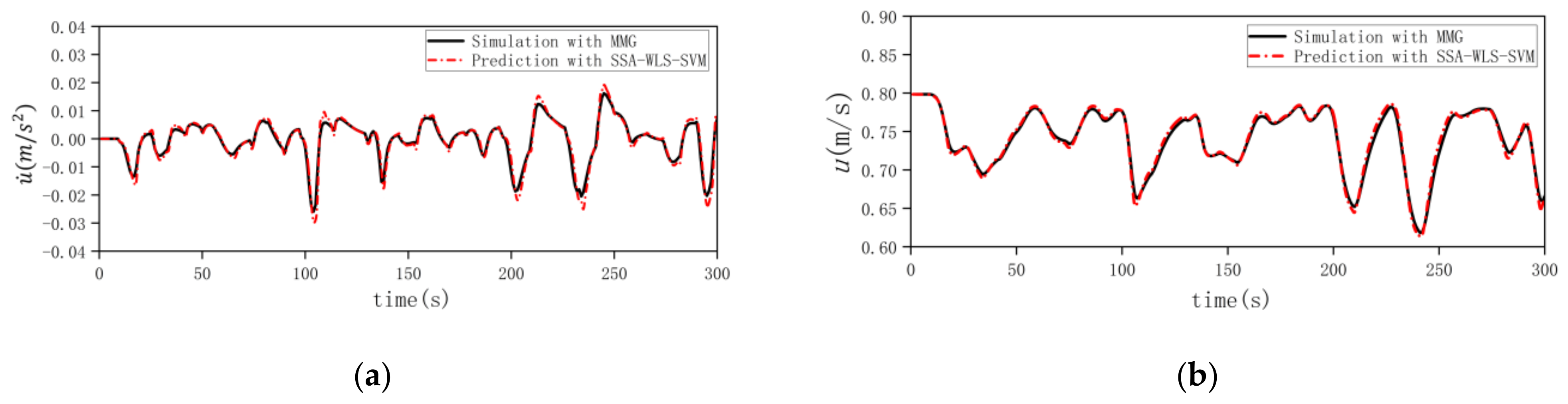
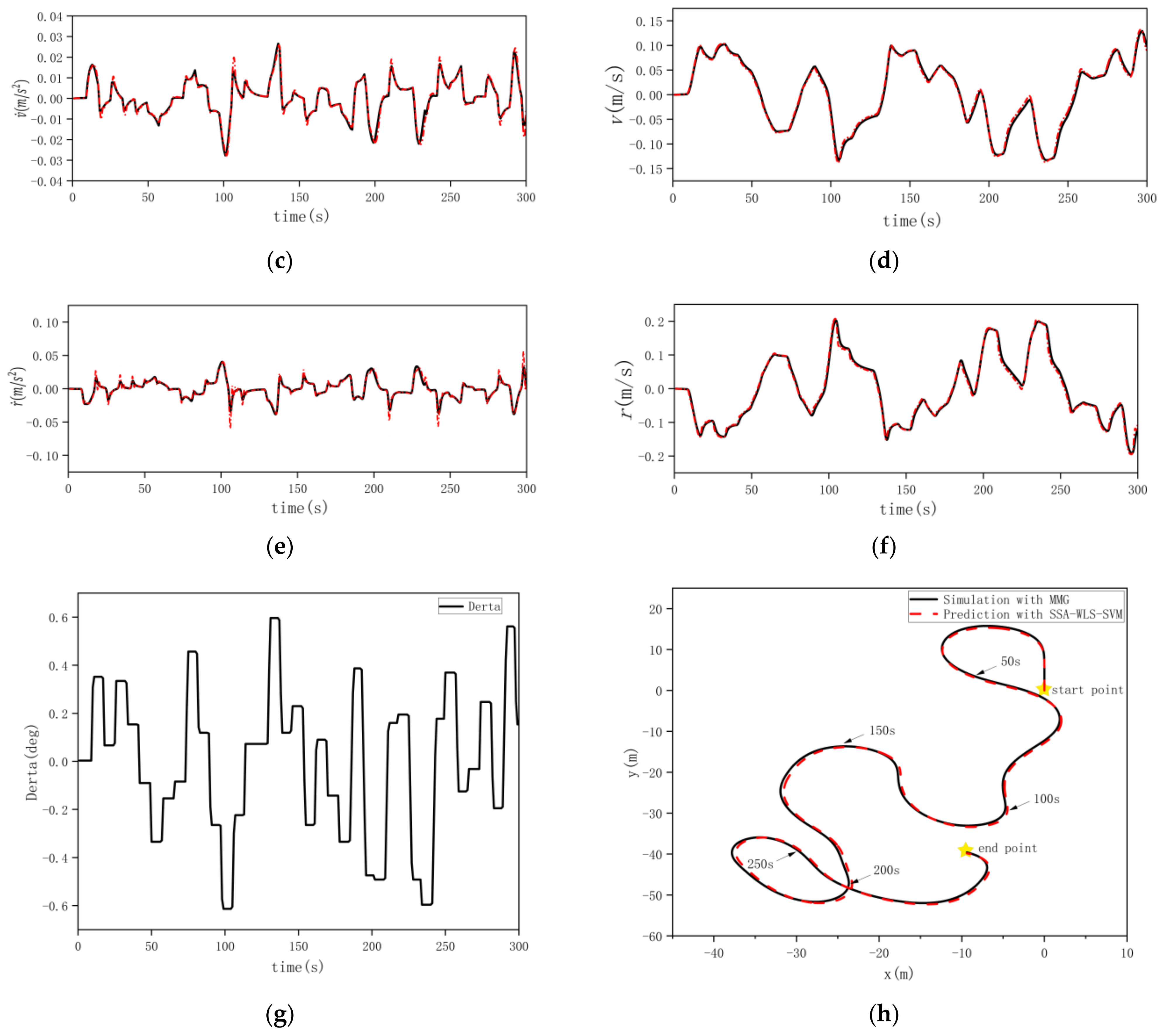
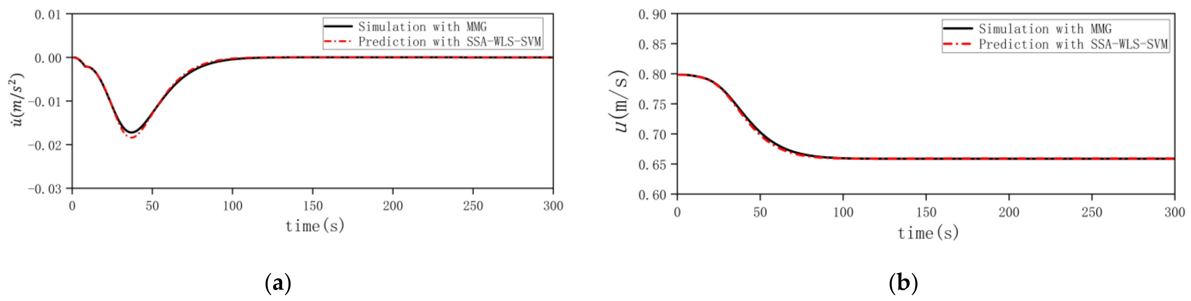
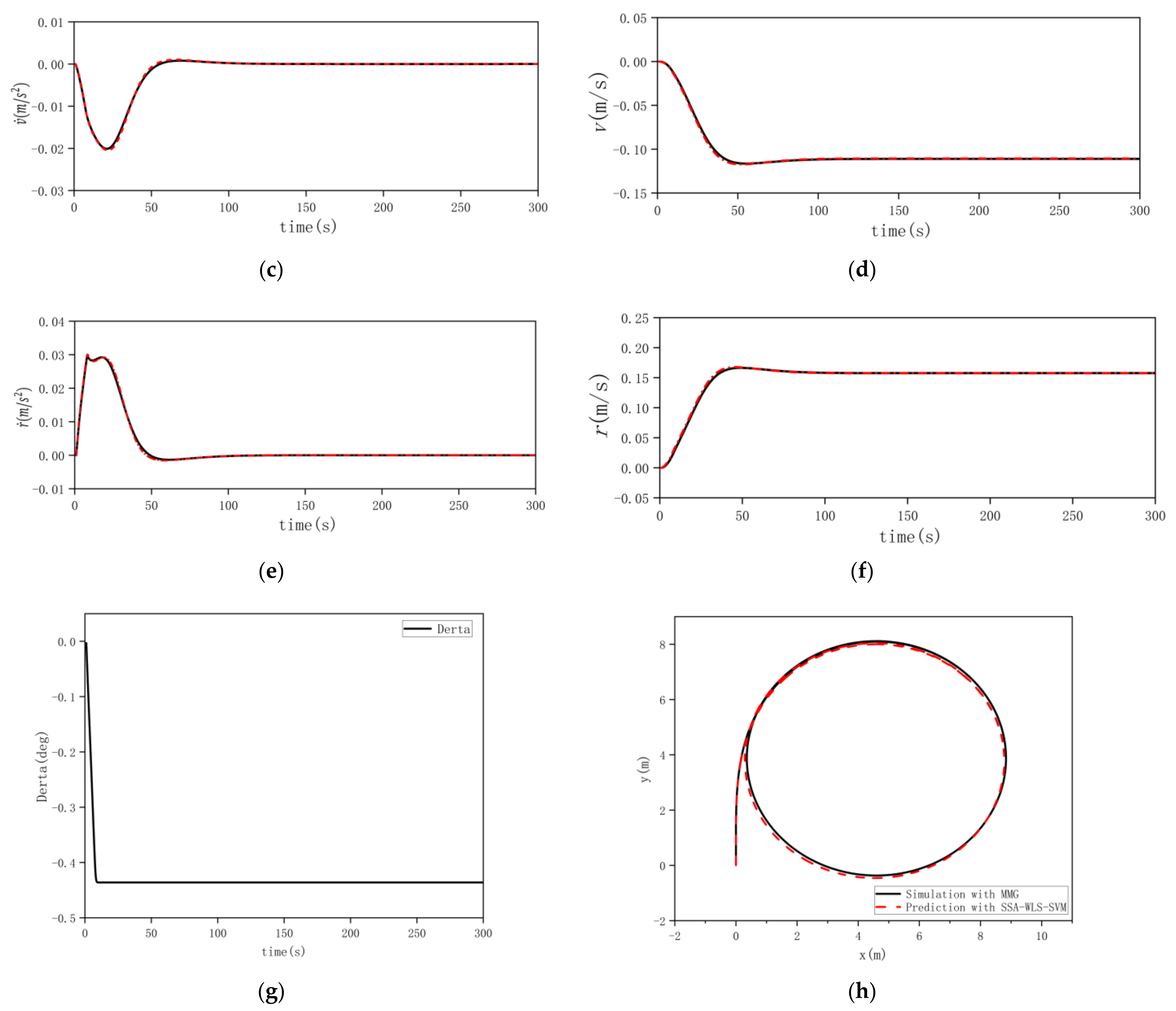
5.3. Model Generalization Verification

In order to verify the generalization performance of the black-box modeling based on SSA-WLS-SVM, the trained black-box model was tested on datasets No. 2 and No. 3. In the prediction process, in the $i_{th}$ step, $\left[u\left(i\right),v\left(i\right),r\left(i\right),\delta \left(i\right)\right]$ was inputted and the corresponding $\left[\dot{u}\left(i\right),\dot{v}\left(i\right),\dot{r}\left(i\right)\right]$ can be outputted, with which the input vector $\left[u\left(i+1\right),v\left(i+1\right),r\left(i+1\right)\right]$ in the next step can be calculated. Therefore, the initial USV status $\left[u\left(0\right),v\left(0\right),r\left(0\right),\delta \left(0\right)\right]$ is the only thing needed for predicting the entire maneuvering motion. Comparison of the SSA-WLS-SVM black-box prediction results and the MMG-model simulation results in Figure 13 and Figure 14 illustrate that the black-box modeling prediction method based on SSA-WLS-SVM has a satisfactory generalization performance.

The root mean squared error (RMSE) and the correlation coefficient (CC) are two main evaluation criteria used to measure the accuracy of the prediction. The RMSE and CC of longitudinal velocity $u$, lateral velocity $v$, and steering angular speed $r$ in random maneuvering dataset No. 1 and No. 2 and 25° turning maneuvering dataset No. 3 are listed in

Table 4. Prediction accuracy of the USV test.

Type of Test	RMSE			CC
	u	v	r	u	v	r
random maneuver set1	4.92 × 10−3	5.43 × 10−3	1.07 × 10−2	0.99383	0.99696	0.99382
random maneuver set2	4.25 × 10−3	7 × 10−3	1.08 × 10−2	0.9880	0.9915	0.9878
25° turning circle maneuver set	2.15 × 10−3	1.19 × 10−3	1.64 × 10−3	0.9989	0.9991	0.9990

. It can be concluded that black-box modeling based on the SSA-WLS-SVM method performs well in predicting the 3-DOF ship maneuvering motion.

6. Conclusions

In this paper, the SSA-WLS-SVM prediction method is proposed to study the USV maneuver prediction under random maneuvering and turning maneuvering. A comparison between the 35° turning maneuvering of the experimental test and the simulation of the 3-DOF MMG model is conducted to prove that the 3-DOF MMG simulation can accurately perform the motion of the USV. Thus, the MMG simulation is used for generating the training data. Meanwhile, the black-box model trained with MMG simulation data is used for the verification of generalizability and accuracy judgment with the USV maneuvering test. The random maneuvering motion and 25° turning circle motion were used as a supplement to verify the generalization performance of the black-box model obtained. The identified results indicate that the trained black-box model has accurate prediction accuracy and a strong generalization performance.

Although the predicted results so far look acceptable, some problems still need to be addressed in future work. In an actual navigation scenario, maneuvering motion modeling is mainly applied to USV motion control, which means an online forecasting is the ultimate goal of USV motion prediction. In this paper, only an off-line 3-DOF maneuvering motion has been modeled and forecasted so far. Thus, an online modeling algorithm with rapid prediction speed should be investigated in further research.

References

1. Marzoughi, A.; Savkin, A.V. Autonomous navigation of a team of unmanned surface vehicles for intercepting intruders on a region boundary. Sensors 2021, 21, 297. [Google Scholar] [CrossRef] [PubMed]
2. Fraga-Lamas, P.; Lopez-Iturri, P.; Celaya-Echarri, M.; Blanco-Novoa, O.; Azpilicueta, L.; Varela-Barbeito, J.; Falcone, F.; Fernandez-Carames, T.M. Design and empirical validation of a bluetooth 5 fog computing based industrial CPs architecture for intelligent industry 4.0shipyard workshops. IEEE Access 2020, 8, 45496–45511. [Google Scholar] [CrossRef]
3. Yuan, X.Y.; Huang, C.Y.; Peng, Y.; Qu, D.; Liu, D. Hierarchical model identi6cation method for unmanned surface vehicle. J. Shanghai Univ. (Nat. Sci. Ed.) 2020, 26, 896–908. [Google Scholar]
4. Bi, H.; Gao, C.; Ma, Y. Research on the legal status of un-manned surface vehicle. J. Phys. Conf. 2018, 1069, 012004. [Google Scholar] [CrossRef]
5. Yu, J.B.; Hu, Z.Q.; Gen, L.B.; Yang, Y. Prediction Method Research on Motion Attitude of Unmanned Semi—Submersible Vehicle. Comput. Integr. Manuf. Syst. 2018, 35, 251–256. [Google Scholar] [CrossRef]
6. Jiang, F.; Li, Y.B.; Yan, F.C.; Gong, J.Y.; Wang, M.Y. Prediction and characteristics of maneuvering performance for asymmetric catamaran based on OpenFOAM. Shipbuild. China 2021, 62, 14–24. [Google Scholar]
7. Liu, Y.; Zou, L.; Zou, Z.; Guo, H. Predictions of ship maneuverability based on virtual captive model tests. Eng. Appl. Comput. Fluid Mech. 2018, 12, 334–353. [Google Scholar] [CrossRef]
8. Wang, X.; Zou, Z.; Xu, F. Modeling of ship manoeuvring motion in 4 degrees of freedom based on support vector machines. In Proceedings of the International Conference on Offshore Mechanics and Arctic Engineering, Nantes, France, 9–15 June 2013; American Society of Mechanical Engineers: Houston, TX, USA, 2013; Volume 55430, p. V009T12A030. [Google Scholar]
9. Carrillo, S.; Contreras, J. Obtaining first and second order nomoto models of a fluvial support patrol using identification techniques. Ship Sci. Technol. 2018, 11, 19–28. [Google Scholar] [CrossRef]
10. Luo, W.L.; Zou, Z.J. Identification of response models of ship maneuvering motion using support vector machines. J. Ship Mech. 2007, 11, 832–838. [Google Scholar]
11. Luo, W.L.; Zou, Z.J. Parametric identification of ship maneuvering models by using support vector machines. J. Ship Res. 2009, 53, 19–30. [Google Scholar] [CrossRef]
12. Luo, W.L.; Zou, Z.J. Analysis of Captive Model Oblique Towing Test by Using Least Squares Support Vector Machines. Shipbuild. China 2010, 51, 10–14. [Google Scholar]
13. Xu, H.; Soares, C.G. Hydrodynamic coefficient estimation for ship manoeuvring in shallow water using an optimal truncated LS-SVM. Ocean Eng. 2019, 191, 106488. [Google Scholar] [CrossRef]
14. Xu, H.; Hinostroza, M.A.; Wang, Z.; Guedes Soares, C. Experimental investigation of shallow water effect on vessel steering model using system identification method. Ocean Eng. 2020, 199, 106940. [Google Scholar] [CrossRef]
15. Xu, H.; Hassani, V.; Guedes Soares, C. Uncertainty analysis of the hydrodynamic coefficients estimation of a nonlinear manoeuvring model based on planar motion mechanism tests. Ocean Eng. 2019, 173, 450–459. [Google Scholar] [CrossRef]
16. Pandey, J.; Hasegawa, K. Study on turning manoeuvre of catamaran surface vessel with a combined experimental and simulation method. IFAC-PapersOnLine 2016, 49, 446–451. [Google Scholar] [CrossRef]
17. Luo, W.; Zhang, Z. Modeling of ship maneuvering motion using neural network. J. Mar. Sci. Appl. 2016, 15, 426–432. [Google Scholar] [CrossRef]
18. Liu, C.D.; Zhang, H.; Han, Y. Black-box modeling and prediction of ship maneuverability based on least square support vector machine. J. Ship Mech. 2013, 17, 872–877. [Google Scholar]
19. Xu, F.; Zou, Z.J.; Xu, X.; Yin, J. Black-box modeling of ship manoeuvring motion based on support vector machines. J. Beijing Univ. Aeronaut. Astronaut. 2013, 39, 1553–1557. [Google Scholar]
20. Bonci, M.; Viviani, M.; Broglia, R.; Dubbioso, G. Method for estimating parameters of practical ship manoeuvring models based on the combination of RANSE computations and System Identification. Appl. Ocean. Res. 2015, 52, 274–294. [Google Scholar] [CrossRef]
21. Sun, X.L.; Xu, F.; Huang, C.; Yang, C.L. Black-box modeling of underwater vehicle’s maneuvering motion based on model test. Ship Sci. Technol. 2018, 40, 75–77,129. [Google Scholar] [CrossRef]
22. He, H.; Zou, Z. Black-Box Modeling of Ship Maneuvering Motion Using System Identification Method Based on BP Neural Network. In Proceedings of the ASME 2020 39th International Conference on Ocean, Offshore and Arctic Engineering, Virtual, Online, 3–7 August 2020; Volume 6B, p. V06BT06A037. [Google Scholar] [CrossRef]
23. He, H.W.; Wang, Z.; Zou, Z.J.; Liu, Y. System Identification Based on Completely Connected Neural Networks for Black-Box Modeling of Ship Maneuvers. In Advances in Guidance, Navigation and Control; Yan, L., Duan, H., Yu, X., Eds.; Lecture Notes in Electrical Engineering; Springer: Singapore, 2022; Volume 644. [Google Scholar] [CrossRef]
24. Zhang, Y.Y.; Wang, Z.H.; Zou, Z.J. Black-box modeling of ship maneuvering motion based on multi-output nu-support vector regression with random excitation signal. Ocean. Eng. 2022, 257, 111279. [Google Scholar] [CrossRef]
25. Liu, Y.; Xue, Y.; Huang, S.; Xue, G.; Jing, Q. Dynamic Model Identification of Ships and Wave Energy Converters Based on Semi-Conjugate Linear Regression and Noisy Input Gaussian Process. J. Mar. Sci. Eng. 2021, 9, 194. [Google Scholar] [CrossRef]
26. Gupta, P.; Rasheed, A.; Steen, S. Ship performance monitoring using machine-learning. Ocean. Eng. 2022, 254, 111094. [Google Scholar] [CrossRef]
27. Gu, S.; Zhu, M.; Chen, G.; Wen, Y.; Knoll, A. Computing position error margin for a USV due to wind and current with a trajectory model. Ocean. Eng. 2022, 262, 111950. [Google Scholar] [CrossRef]
28. A robust localization algorithm in wireless sensor networks. Comput. Sci. 2008, 2, 438–450. [CrossRef]
29. Gezici, S.; Kobayashi, H.; Poor, H.V. Non-parametric non-line-of-sight identification. In Proceedings of the 2003 IEEE 58th Vehicular Technology Conference, VTC 2003-Fall (IEEE Cat. No.03CH37484), Orlando, FL, USA, 6–9 October 2003; Volume 4, pp. 2544–2548. [Google Scholar]
30. Ji, Y.B.; Qin, S.R.; Tang, B.P. Digital Filtering with Zero Phase Error. J. Chongqing Univ. (Nat. Sci. Ed.) 2000, 23, 4–7. [Google Scholar] [CrossRef]
31. Savitzky, A.; Golay, M.J.E. Smoothing and differentiation of data by simplified least squares procedures. Anal. Chem. 1964, 36, 1627–1639. [Google Scholar] [CrossRef]
32. Xu, X.Y.; Zhong, T.Y. Construction and Realization of Cubic Spline Interpolation Function. Autom. Meas. Control. 2006, 25, 76–78. [Google Scholar] [CrossRef]
33. Vapnik, V. The Nature of Statistical Learning Theory; Springer Science & Business Media: Berlin/Heidelberg, Germany, 1999. [Google Scholar]
34. Zhou, Z.H. Machine Learning; Springer: Berlin/Heidelberg, Germany, 2016. [Google Scholar]
35. Suykens JA, K.; Vandewalle, J. Least squares support vector machine classifiers. Neural Process. Lett. 1999, 9, 293–300. [Google Scholar] [CrossRef]
36. Suykens, J.A.; De Brabanter, J.; Lukas, L.; Vandewalle, J. Weighted Least Squares support Vector Machines: Robustness and sparse approximation. Neurocomputing 2002, 48, 85–105. [Google Scholar] [CrossRef]
37. Suykens, J.A.K.; Lukas, L.; Vandewalle, J. Sparse least squares Support Vector Machine classifiers. In Proceedings of the 2004 IEEE International Joint Conference on Neural Networks (IEEE Cat. No.04CH37541), Budapest, Hungary, 25–29 July 2004; pp. 37–42. [Google Scholar]
38. Hampel, F.; Ronchetti, E.; Rousseeuw, P.; Stahel, W. Robust Statistics: The Approach Based on Influence Functions; Wiley: New York, NY, USA, 1986. [Google Scholar]
39. Xue, J.K.; Shen, B. A novel swarm intelligence optimization approach: Sparrow search algorithm. Syst. Sci. Control. Eng. 2020, 8, 22–34. [Google Scholar] [CrossRef]
Figure 1. Body coordinate system of a USV.
Jmse 11 00324 g001
Figure 2. Geometric model and physical model of the USV (a) geometric shape (b) model of the USV.
Jmse 11 00324 g002
Figure 3. Compute grid.
Jmse 11 00324 g003
Figure 4. Resistance of the USV in direct navigation.
Jmse 11 00324 g004
Figure 5. Wave shape (Fourier coefficient: left: 0.2, middle: 1, right: 1.6). Different colors represent different wave heights, which gradually decrease from the tail to the distance.
Jmse 11 00324 g005
Figure 6. Coupled ripple of oblique motion and circumferential motion (left: dimensionless steering angular speed is 0.4, drift angle is 0 degrees; middle: dimensionless steering angular speed is 0.4, drift angle is −10 degrees; right: dimensionless steering angular speed is 0.8, drift angle is −10 degrees).
Jmse 11 00324 g006
Figure 7. Test Platform Architecture Diagram (a) Establishment of the test coordinate system; (b) Schematic diagram of data transmission on the hardware platform.
Jmse 11 00324 g007
Figure 8. Schematic diagram of the RRF.
Jmse 11 00324 g008
Figure 9. Comparison results of different data processing methods (a) Comparison results of the resultant speed. (b) Comparison results of the position.
Jmse 11 00324 g009
Figure 10. Comparison of the prediction and experiment in the 30° turning circle. (a) Speed comparison. (b) Track comparison.
Jmse 11 00324 g010
Figure 11. SSA-WLS-SVM Black-Box Model motion prediction process.
Jmse 11 00324 g011
Figure 12. Comparison of the prediction with SSA-WLS-SVM and simulation in dataset 1. (a) Longitudinal acceleration. (b) Longitudinal velocity. (c) Lateral acceleration. (d) Lateral velocity. (e) Steering angular acceleration. (f) Steering angular speed. (g) Rudder angle. (h) Track of USV.
Jmse 11 00324 g012aJmse 11 00324 g012b
Figure 13. Comparison of the prediction with SSA-WLS-SVM and simulation in dataset 2. (a) Longitudinal acceleration. (b) Longitudinal velocity. (c) Lateral acceleration. (d) Lateral velocity. (e) Steering angular acceleration. (f) Steering angular speed. (g) Rudder angle. (h) Track of USV.
Jmse 11 00324 g013aJmse 11 00324 g013b
Figure 14. Comparison of the prediction with SSA-WLS-SVM and simulation of the 25° turning maneuvering motion. (a) Longitudinal acceleration. (b) Longitudinal velocity. (c) Lateral acceleration. (d) Lateral velocity. (e) Steering angular acceleration. (f) Steering angular speed. (g) Rudder angle. (h) Track of USV.
Jmse 11 00324 g014aJmse 11 00324 g014b