

Statutory and Operational Damage Stability by a Monte Carlo Based Approach
Institute of Ship Design and Ship Safety, Hamburg University of Technology, 21073 Hamburg, Germany
J. Mar. Sci. Eng. 2023, 11(1), 16; https://doi.org/10.3390/jmse11010016
Submission received: 28 October 2022
/
Revised: 14 December 2022
/
Accepted: 15 December 2022
/
Published: 22 December 2022
(This article belongs to the Special Issue Damage Stability of Ships)
Abstract
:The paper describes the extension of a Monte Carlo based damage stability simulation method for the generation of approval documents for both statutory and operational damage stability. The intention of this development is that the advantages of the Monte Carlo damage stability simulation concept can be used without the necessity to ask for alternative design approval procedures during the statutory approval by the classification society. This means that the same damage stability documentation must be generated as by the conventional damage stability calculation. To generate the required approval documentation, the individual probabilities for each damage case have to be determined and the different damage cases have to be sorted into so called damage zones, which is required by the classification societies. Within one damage zone, the splitting of damage cases was found to be necessary to avoid the computation of probabilities greater than 1. This extended method is then applied to the computation of damage stability during the operation of ships, which means that the method can now be applied in situ to real loading conditions, which makes the ship operation more flexible. This new capability is also interesting for those ships which carry a substantial amount of project deck cargo.
1. Introduction
Damage Stability Problems for ships are quite time consuming with respect to damage modeling and computation times, especially during the initial design phase, when many of these calculations have to be performed during the various design loops. To overcome this problem, a Monte Carlo-based simulation procedure for damage stability problems was developed over the years which treats damage stability as a stochastic process. This method is successfully in use during the design phase of the ship.
If this very efficient simulation principle shall now also be used after the design phase for the generation of approval documents, additional information needs to be generated by this method which is not directly obtained by the simulation principle. Because this additional information is strictly required by the classification societies. There is principally the option to ask for a so called “alternative design” approval, which may result in deviations from the normal approval procedures and which may then allow a Monte-Carlo simulation principle instead of conventional computations. However, this is more time consuming and also more expensive, and it is therefore not seen as practical alternative for the daily business of a shipyard’s design office.
The major drawback of the Monte Carlo Simulation has been that it does not deliver the damage zones (the simulation is a nonzonal approach) which are required to verify the calculation during the approval phase. Where a damage zone is typically defined as the longitudinal distance between two transversal subdivision elements, e.g., bulkheads. Further, the individual damage probabilities in length, in penetration and in height are not known explicitly, as the Monte-Carlo simulation delivers only the total product of these three probabilities. These probability values, depending on the defined damage zones, need to be obtained and documented for the final approval of the calculation results. This problem has now been overcome, and the solution of this problem will be described briefly in the paper.
This extended Monte Carlo-simulation method is then applied to the computation of damage stability during the operation of ships, which means that the method can alternatively be applied in situ to real loading conditions, including filled tanks and cargo spaces, where the required index can be obtained from the approved stability booklet for the analyzed loading condition. The paper will show that this allows for a much more flexible operation of ships, especially for those types of ship which operate at lower drafts with a significant amount of deck cargo.
2. Background
Probabilistic damage stability calculations require both a substantial modeling effort and computational time. Besides hull form and compartmentation, all relevant openings need to be included in the computational model. After the computational model has been set up, the conventional calculation procedure is as follows: for a given compartment or group of compartments, the probability Pi that this compartment or group of compartments is damaged needs to be calculated according to the SOLAS 2020 B1 regulations as follows:
Pi(x1,x2,y,z) = pi(x1,x2) ri(y,x1,x2) vi(z)
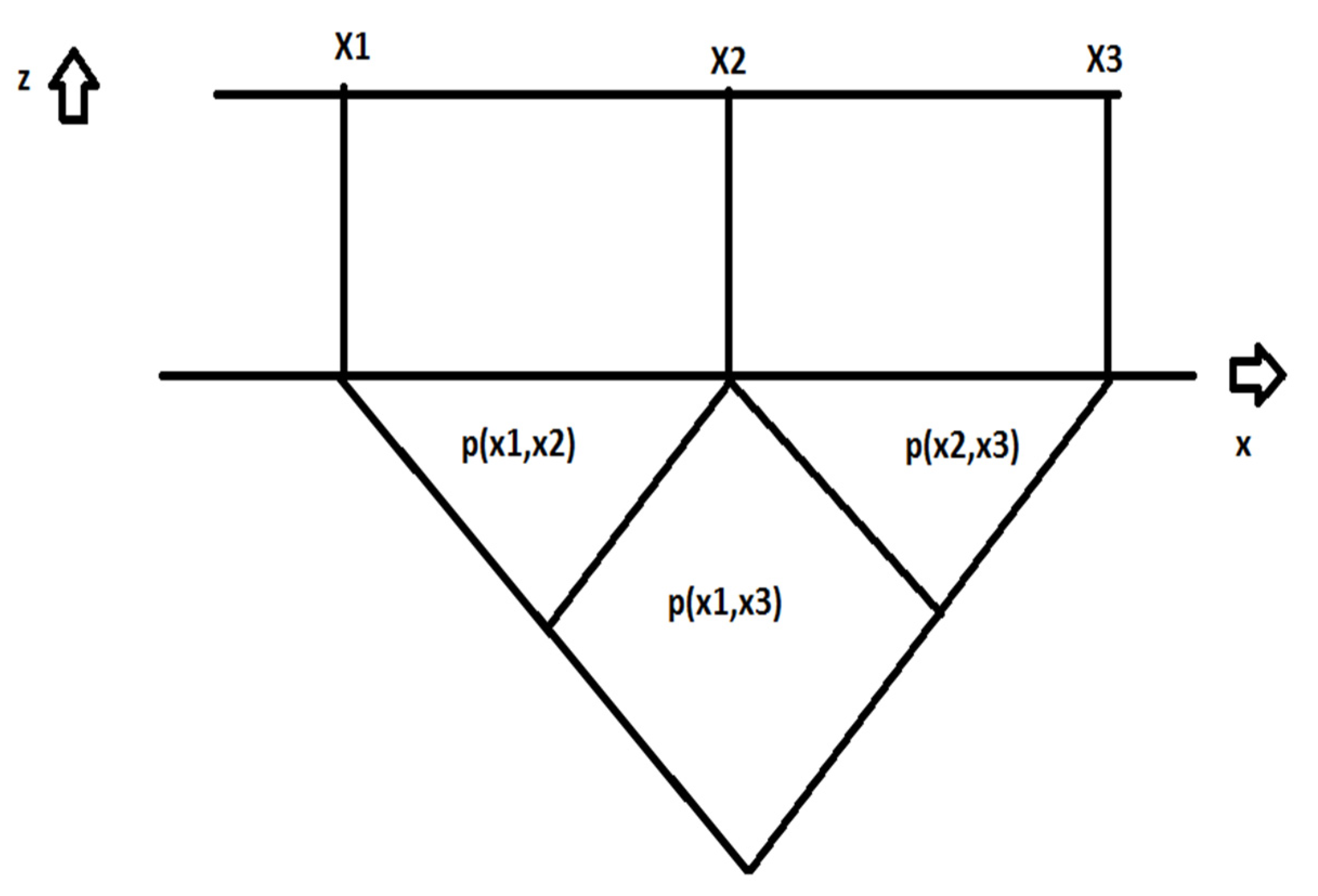
In Equation (1), Pi denotes the total probability that the compartment or group of compartments is damaged. The individual probabilities pi, ri, and vi are related to the damage cuboid which extends from x1 to x2 in longitudinal direction. The transversal penetration depth is y, measured from the damage waterline, and the vertical extension is from the base line to the damage height is z. pi(x1,x2) is the probability that the damage extends from the aft position located at x1 to the forward position x2. ri(y) is the probability that the penetration depth extends to the local breadth y and vi(z) is the probability that the damage extends to the height z. Formula (1) is applicable for so called one-compartment damages (see Figure 1), and it should be noted that the probability ri is depending not only on the penetration depth, but also on the length of the damage as given by x1 and x2. Further, the SOLAS requires also to investigate damages where the lower boundary in z is above the baseline (so called lesser extent cases), but this investigation is performed during the calculation of the individual Si-factors (survivability of the damage) according to the SOLAS requirements.
If now a two-compartment damage is to be considered with transversal bulkheads located at x1, x2, and x3, the probability pi,2 for a damage which opens only the two compartments (and not a single compartment) is to be calculated as follows (see Figure 1):
pi,2(x1,x3) = pi(x1,x3) − pi(x1,x2) − pi(x2,x3)
This means that the probabilities of the two one-compartment damages are required to compute the probability of a two-compartment damage. If three-compartment damages have to be calculated, all two- and one-compartment damages are required. The same holds for four-, five-compartment damage cases and so on. After the determination of pi, the penetration depth y and damage height z need to be considered to obtain the probabilities ri and vi. When the total probability Pi of the damage case has been determined from the combination of Formulae (1) and (2), the probability of survival Si needs to be computed. This requires a hydrostatical analysis of the damage case. The product Pi Si then contributes to the total attained index A. If that index A is larger than the required index R, the calculation is finished. The calculation has to be made for three drafts, assuming damages from both port and starboard side. It has to be repeated many times during the design of a ship, as many variations of possible compartmentations in combination with possible values of GM have to be investigated. As a matter of fact, this process is quite inefficient with respect to modeling effort and also computational time. At first, the manual input of longitudinal damage zones, penetration depths and damage heights results in the fact that the ship’s compartmentation is actually modelled twice, which boosts the modeling effort. If during the design phase of the ship the compartmentation is modified, each modification must be reprocessed in the modeling of the damage cases. Besides possible consistency errors, this requires a lot of time. For this reason, the damage stability calculation process has been reengineered in our ship design software by inverting the problem, see Krüger and Dankowski [1]. Comparable developments have been made by Koelmann [2], Bulian [3,4,5,6], Ruponen [7], and Mauro [8]. This inverted method is based on the concept that instead of assuming a damage case and calculating the related probabilities, it is much more efficient to assume a damage extent and to compute the outcome of that particular damage extent, which can be most efficiently solved by a classical Monte Carlo Simulation technique. This method has been proven as a very efficient tool during the design phase of a ship, as the A-index and the limiting stability curves can be calculated extremely fast. The problem now exists that despite these improvements, still a significant amount of man hours is required to generate the approval documents, even if the compartmentation and the limiting stability curves are already fixed. Therefore, it would be extremely useful if this efficient simulation principle could be extended for the generation of approval documents. This requires the generation of additional data which cannot directly be obtained from the Monte Carlo simulation method. Most challenging here is to determine the required individual probabilities p, r, and v, to sort damage cases into damage zones and to split damage cases afterwards according to their individual penetration depths. The following sections give an overview about this development, which is a kind of reverse engineering of the conventional calculation principle based on the Monte Carlo simulation. First, the Monte Carlo simulation principle is briefly introduced.
3. Monte Carlo Realization
The Monte Carlo simulation principle for damaged ship problems was proposed by Koelmann [2] for damage stability problems and by Kehren [9] for the oil outflow problem of the MARPOL regulations. In 2015, Bulian et al. [3] applied that principle also to grounding problems with further and deeper research into that problem in 2020 [3]. In 2019 Bulian, Ruponen et al. [4] refined this approach to a general damage stability concept. Ruponen et al. [7] and Dankowski [10] have combined a Monte Carlo simulation with a time domain flooding simulation to obtain the survivability of a passenger ship. Santos and Guedes Soares [11] applied this approach to the damage stability of a RoRo-Ship. One can therefore most probably say that this principle is well established for damage stability problems since many years and it is applied by many researchers in the field of modern ship theory. Recently, Mauro and Vassalos [8] described a concept to improve the sampling method of the MC-simulation to further reduce the computational effort.
Although this principle has shown many advantages, it is according to the author’s knowledge commonly not in use for the generation of statutory damage stability approval documentation, e.g., according to the SOLAS 2020 B1. This is because the approval process in practice requires information that is difficult to obtain from a Monte Carlo simulation principle. This particular problem is addressed in the following sections. Beforehand, a short description of the basic Monte Carlo simulation principle for damage stability problems is given.
Each statistical process can be described by a distribution function (also called the cumulative density function CDF). These distributions are based on known damage statistics [12]. These damage statistics are the basis for the existing SOLAS 2020 B1, which is principally identical with the SOLAS 2009. Cumulative density functions are given for the damage length, damage location, penetration, and damage height. According to the assumptions of SOLAS 2020 B1 [13], the lower damage boundary is 0 (base line of the ship), but possible lesser extending damage cases have to be investigated in addition during the Si computations according to the principles stated in the SOLAS. Bulian et al. [6] have shown an interesting alternative method to include other lower damage boundaries than base line in the Monte Carlo simulation, but this would deviate from the SOLAS and would then require alternative approval procedures.
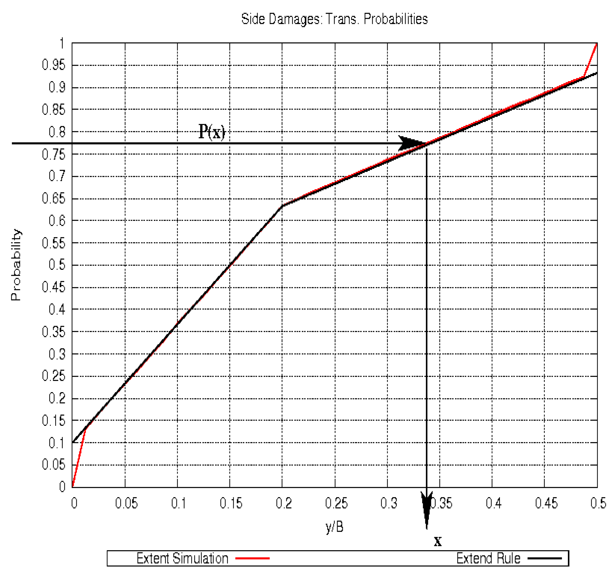
The principle of the Monte Carlo simulation is now simply to ask for the inverse of such a kind of function, see Figure 2, which shows the cumulative density function for the penetration depth as an example. By using a uniformly distributed random number generator [14], a value between zero and one is chosen. This random number is considered as a probability and the corresponding event is selected from the distribution. If this is repeated with a sufficient number of samples, these events will converge to the original underlying distribution. The number of events (or frequencies) in discrete intervals are counted by a simple yes/no selection. Integrating the resulting data leads to almost the same as the underlying distribution. In addition, the confidence interval can be computed, which shows the statistical accuracy depending on the number of samples.
Using this approach, the generation of the required damage cases simply boils down to the generation of a sufficient number of damage cuboids according to the given statistical distribution. Each damage cuboid breaches a certain combination of ship compartments (damage case). Counting the number of hits for each damage case and dividing it by the total number leads to the encountered frequency of that particular damage case. The procedure can be summarized as follows:
- Draw the damage cuboid from the damage distributions.
- Find the corresponding damage case.
- Integrate the hits for each individual damage case.
After a sufficient number of drawings, the frequency for each damage case is simply the number of hits divided by the total number of samples. This method is actually very simple and it has got the following advantages compared to the conventional method:
- The number of hits even for a very complex combination of compartments can directly be computed. There is no need to look at any subcases and their probabilities.
- As counting of hits is simply a binary event (yes/no), also very complicated geometries can easily be handled (in contrast to the procedure described in the SOLAS Explanatory Notes, which is in parts reflected by Figure 1).
- Sorting the damage cases according to the frequency gives direct access to the important cases for the subdivision design. This shows the designer immediately which compartment combinations have the largest impact on the subdivision index A.
- Additionally, substantially more damage cases will be found compared to the conventional method. For sufficiently large samples, all possible damages cases are found by the simulation. This is very important for validation purposes.
After the generation of the damage cases, the survivability for each damage case Si can be computed according to the regulations in the SOLAS. The only requirements for this method are the damage distribution functions, a random number generator (e.g., Matsumoto [14]), and a reliable method to obtain the combination of damaged compartments from the geometry of the damage cube. It was shown by Kehren [9] that the obtained probabilities do clearly converge for large numbers of samples. For practical damage stability assessments, a sufficiently large sample is assumed to be 1.0 × 10⁶ drawings. As shown by Dankowski and Krüger [1], this simulation method shortens the damage stability computation time drastically and the method has successfully been applied during the initial design phase of complex ship subdivisions by the industry.
However, for the generation of damage stability approval documents, the proposed method has two major drawbacks:
- It can only deliver the total probability pi(x1,x2) ri(y,x1,x2) vi(z) and not the individual probabilities pi, ri, and vi. However, the calculation of the individual probabilities is required for the approval by the classification societies.
- The output of the method consists of individual damage cases with their contribution to the total index. For the generation of approval documents, it is necessary to group the damage cases into so called damage zones, which can be defined either by the user or (as a default) by a program. All damage cases located in a damage zone must then be sorted according to their damage heights and their penetrations.
In the following, we will show that the solution of both problems is closely linked together, and they must be solved simultaneously. We will show that during the solution of these problems, another difficulty will occur, namely that the probability ri can in some cases take values larger than 1 which requires further measures to solve this problem.
4. Determination of the Probabilities Pi, Ri and Vi
4.1. Principle Approach
We will in the following show that there are three key issues necessary to solve the aforementioned problems:
- The determination of the probability pi by an additional drawing.
- The adding of damage zones.
- The splitting of damage cases to cope with probabilities ri that are larger than 1.
The determination of the probability pi requires a modification of the Monte Carlo simulation method. This modification is described in the following: From Equation (1) it becomes obvious, that ri(y,x1,x2) and vi(z) become exactly 1 if the damage cuboid extends to the maximum possible damage height zmax and maximum possible damage penetration ymax. If now ri(ymax,x1,x2) = 1 and vi(zmax) = 1 hold, then it becomes immediately obvious that Pi(x1,x2,ymax,zmax) = pi(x1,x2), which means that our simulation principle will determine the probability pi(x1,x2) instead of the total probability Pi(x1,x2,y,z). This does in practice mean that we have to modify the simulation principle by adding so called “fully extent damage cases” which are obtained from a second drawing with a modified cuboid as follows: before we determine the damage case from the cuboid extensions as obtained from the underlying CDF data, we modify each damage cuboid by setting z = zmax and y = ymax. From this additional cuboid we can obtain the combination of compartments breached by this “fully extent” cuboid and we obtain the so called “fully extent damage case”. If we do now integrate the hits for each full extent damage case, we can obtain the probability in the same way as before. However, we do know that this probability must be equal to pi(x1,x2), as ri and vi are 1 by definition. As we do perform both drawings simultaneously, we know for each individual damage case to which full extent damage case it belongs, and consequently, we know the probability pi(x1,x2) for all these damage sub cases.
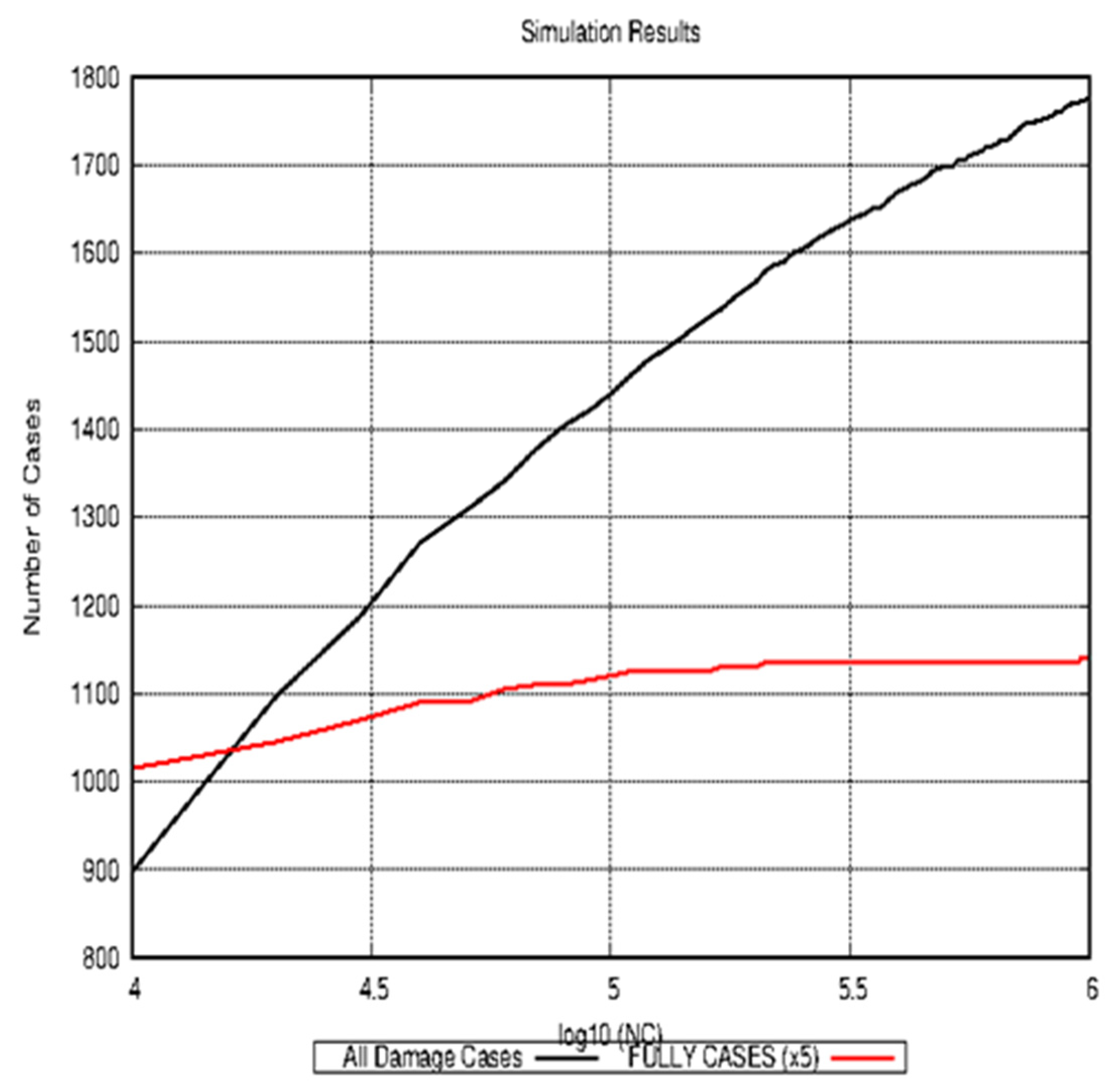
This principle will in the following be applied to the investigation of the damage stability of the EMSA2-reference vessel [15]. Figure 3 shows some interesting facts for the EMSA2-RoPax. The x-axis represents the log10 of the sample number N, which is the number of drawn cuboids. The black curve shows the number of damage cases which were obtained from the simulation. The red curve shows the number of full extent damage cases multiplied by a factor of 5 for the sake of better visibility. One can immediately see that the total number of full extent cases quickly converges to a number of 228 (1140/5), whereas the number of all damage cases has not finally converged. This shows that our simulation with 1.0 × 10⁶ samples has most probably detected all possible full extent configurations, but there should be remaining combinations of penetration depths and damage heights which have not yet been detected. However, from a practical viewpoint, this is not a problem because the index contribution of these remaining cases (even if they would be survived) is in the order of magnitude of about 1.0 × 10⁻⁵. The total number of damages cases with a sample of 1.0 × 10⁶ is 1776, which means that each full extend damage case has in average 7.78 sub damage cases. In fact, the number of sub cases varies from 1 to 34 sub cases for each full extent damage case. By this second drawing, we have now not only established a relationship between a damage case and its full extent damage case, but we can now at the same time compute the required probability pi. All sub cases of all full extent damage cases must then be damage cases where either ri or vi or both do not equal 1. It should be mentioned in this context that the computed index Ai is astonishingly robust: with only 10,000 drawings, one obtains an index of already 0.7222, where the computed index for 1.0 × 10⁶ drawings amounts to 0.7212. The difference is about 1‰.
As a next step, we must now analyze all sub damage cases of each full extent damage case with respect to their individual maximum damage heights and maximum penetration depths. Because both penetration maxima in z and y cannot directly be obtained from the simulation results, as the cuboids do not necessarily extend to both maxima, even if a very large number of cuboids is drawn. To overcome this problem, it was found most efficient to map the upper boundary of all damage cuboids of a damage case to the largest zmax-value of all the spaces of all compartments breached each cuboid. As a consequence, we obtain a reliable value for the maximum damage height z of each individual damage case. Applying the same procedure also for the y-coordinates of each cuboid, we can obtain the maximum penetration depth for each individual damage case. However, this task is now much easier, as we have already pre-sorted the damages according to their individual damage heights. We have decided to start with the damage heights first due to the fact that this direction is geometrically less complex compared to the y-penetration.
Now we can group all damage cases in such a way that each damage penetration may have varying damage heights. If all damage heights for a given penetration depth are known, the individual probabilities vi(z) for each group of penetration depths can directly be computed for each of these individual damage cases from the basic CDF Formulae. As already mentioned, the probability pi is obtained from the full extent case. The remaining probability ri (which is the most challenging one, because it depends on both penetration and damage length) can then simply obtained by inverting Equation (1):
ri(x1,x2,y) = Pi(x1,x2,y,z)/pi(x1,x2)/vi(z)
4.2. Procedural Problems during the Determination of Pi, Ri, and Vi
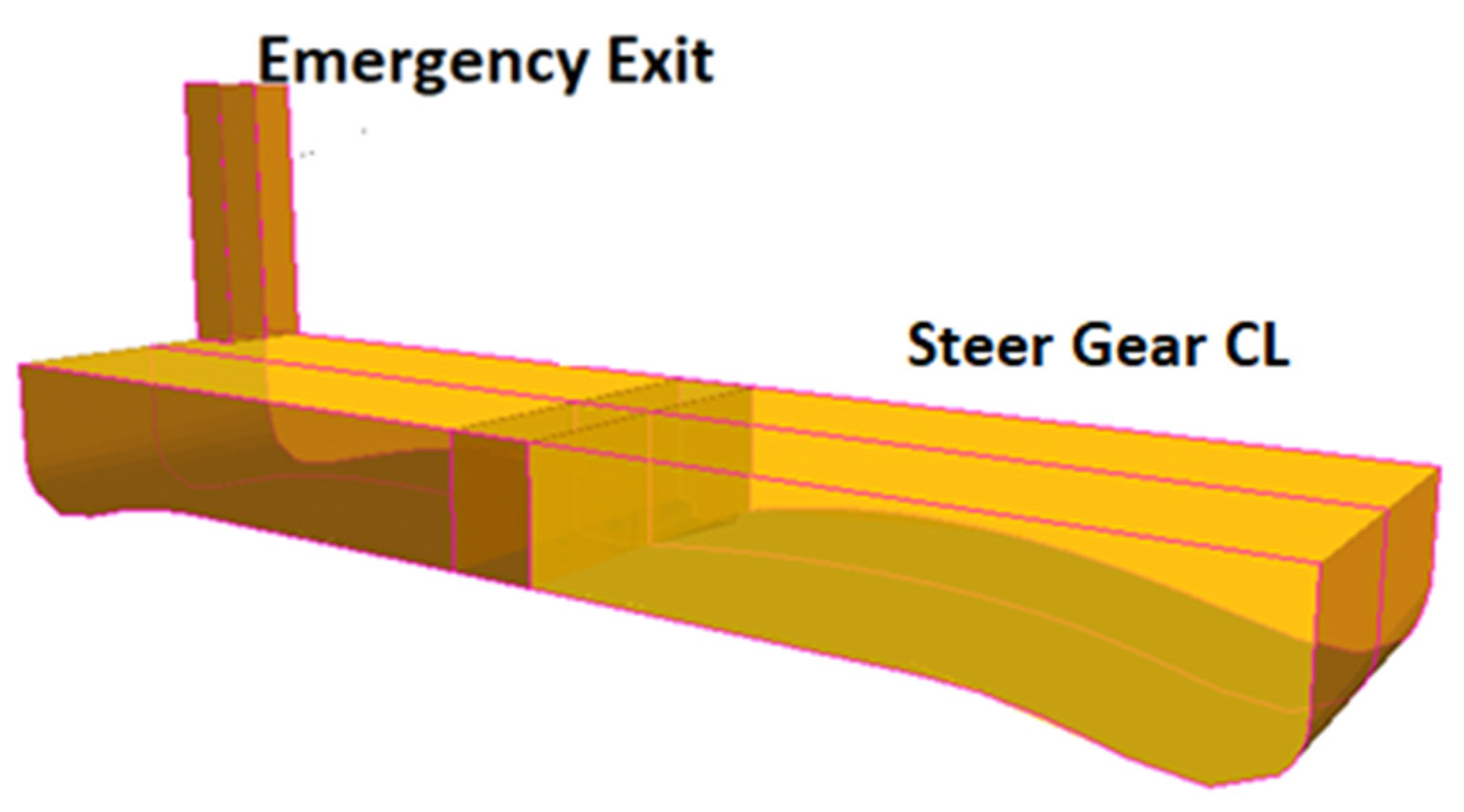
Even if this described principle seems to be straight forward and easy to automate, it cannot always deliver exactly the same individual probabilities as obtained from the manual user input of damage cases, as the following example will show. Figure 4 shows the steering gear compartment of the EMSA2-RoPax. The steering gear compartment is located below the main garage deck at 9.20 m above the base line of the ship. On port side, there is an emergency exit which extends to the superstructure deck at 16.00 m. The watertight compartment “Steering Gear Compartment” consists of the two spaces “Emergency Exit” and “Steer Gear CL”, as shown in Figure 4. The connection between these two spaces is not watertight. For this ship, z = 16.00 m means that vi(z = 16.00) = 1, and at the same time vi(z = 9.20) = 0.2769. The problem now exists that a damage case which does breach only the steering gear compartment (and no other) is possible by two basically different damage types:
- Any damage which does not breach the space “Emergency Exit” but only the space “Steer Gear CL” must have a maximum damage height of less or equal to 9.20 m. The damage penetration is the maximum penetration possible.
- Or the damage breaches only the space “Emergency Exit”, and then the maximum damage height is 16 m with a limited penetration.
The algorithm we have described above would now result in the situation that this case is one sub damage case amongst others for the related full extent damage case. The probability pi(x1,x2) is obtained from the full extent case, and our methodology would result in zmax = 16.20 m for this particular case, resulting in vi = 1 and ri according to Equation (3). This result is obviously a possible and a reasonable result at the same time, but it differs from a conventional damage stability calculation: From the viewpoint of a manual damage case generation, the damage case “steering gear compartment” must be divided into two separate damage zones to correctly obtain the three individual probabilities. The Monte Carlo simulation is due to its principle able to deliver the total probability Pi correctly, but the splitting of the total probability into the three individual probabilities does obviously depend on the splitting of damage cases into longitudinal damage zones. We will later show that a comparable problem exists for the transversal penetration, too. The following subsections show how these difficulties can be overcome in the framework of the Monte Carlo simulation.
4.3. The Necessity of Adding Damage Zones
It was shown above that it is necessary to sort individual damage cases into longitudinal zones if the results shall be comparable to the conventional calculation. The definition of the damage zones is then only parameter that triggers the output of the damage stability analysis (but not the results). Damage zones are defined by giving a minimum and a maximum x-value for each damage zone. These damage zones can either be defined by the user per manual input or they can be generated automatically from the information on the ship’s compartmentation in different granularities.
From the above mentioned, it becomes obvious that it is sufficient to split only the full extent damage cases according to the damage zone definition, because all sub cases of these full extent damage cases must then lie in the same damage zone. Krüger and Dankowski [1] have described an algorithm how the flooded length of a damage obtained from a Monte Carlo simulation can be calculated based on the ship’s compartmentation. The flooded length differs from the damage length, as the flooded length extends from the most rearward to the most forward bulkhead of the damaged compartments. The damage length is obtained from the rearmost position of all damage cuboids of the damage case and the most forward position of all these damage cuboids. Obviously, many damage lengths can lead to the same flooded length, and the damage length is smaller or equal to the flooded length.
This algorithm is now used to obtain the zone based damage lengths of the full extent damage cases, and the obtained damage lengths from all cuboids can then be mapped on the actual damage zone definition. This allows the connection of any full extent damage case to one or more damage zones. If now any randomly drawn damage cuboid detects an already known combination of breached compartments, but in a new damage zone, this combination of damaged compartments is treated like a new damage combination to force that the probabilities are split accordingly. As the compartment combination is identical (but located in another damage zone), the survivability must be the same and needs to computed only once. Adding the damage zones does then neither have an impact on the computed index nor on the computation time, but only on the number of output damage cases, which depends on the granularity of the selected damage zone setup. The computed index A is independent of the damage zone granularity, as the latter forces only the splitting of the individual damage cases into the predefined damage zones. The generation of the damage zone information requires only a little additional effort, but it allows the user to control the output generated by the method according to his requirements. Additionally, it is of course still possible to run the method without damage zones (e.g., during the initial design phase of the ship) when no approval documents need to be generated.
4.4. The Necessity of Splitting Damage Cases in a Damage Zone
We will in this section show that a comparable problem as discussed before does also exist for the transversal direction of the damage, but this problem must be solved differently. In Figure 5 a situation is shown which leads to the fact that the probability ri obtained from Equation (3) may become larger than 1. This is due to the following reason: The void space (and only the void space) can be damaged by principally two different cuboids. One group of cuboids has the full damage height, but the penetration depth is limited to the inner longitudinal bulkhead. If the penetration depth would be larger, then also the lower hold would be damaged, which leads to a different damage case. This set of cuboids is denoted by 1 in Figure 5. Alternatively, the cuboid has a damage height lower than zmin of the lower hold, but a penetration depth which extends to the pipe duct in the center. This set of damage cuboids is denoted by 2 in Figure 5.
During the Monte Carlo Simulation, both damage scenarios appear in the probabilities Pi and pi. After the simulation is finished, these probabilities Pi and pi are correctly determined. When now the product ri vi is analyzed according to the aforementioned procedure, it is found that the maximum damage height of this damage case is surely zmax, which comes from the cuboid group 1. The maximum penetration depth is now the transversal position of the pipe duct, which comes from damage cuboid group 2. However, both extremes at the same time are not possible, because that would result in a different damage case. If now the probability vi is obtained from zmax, this results in the fact that the obtained ri from Equation (3) is now larger than 1, which is due to the fact that r includes contributions from both damage scenarios at the same time. Although the product ri and vi is obtained correctly from the simulation, it is formally difficult to explain that one individual probability shall take a value larger than 1.
To solve this problem, the damage case must be split into two subcases, which is easily possible due to the fact that after the Monte Carlo simulation is performed, all damage cuboids are known. This damage case (damaging only void space 3) is then split into two subcases: one representing cuboid group 1 with the full damage height, but penetration depth equivalent to the inner longitudinal bulkhead, and a second damage case with the lower damage height, but a larger penetration depth equivalent to the pipe duct. For both cases, the individual ri and vi can be obtained. As pi must be the same for both sub cases, the two values of the total probabilities Pi can then be obtained from Equation (1). This splitting of the damage cases can now automatically and iteratively be processed for all situations where ri > 1 is detected.
5. Numerical Studies
The SOLAS 2020 (as well as the SOLAS 2009) prescribes that the basic probability of survival Si is to be computed as
for a damage case of a roro-passenger ship that involves a roro-compartment, and
otherwise.
Si = k (h/0.2 r/20)1/4
Si = k (h/0.12 r/16)1/4
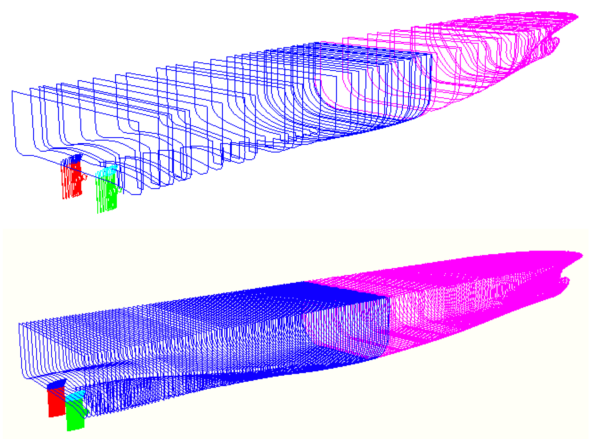
In Formulae (4) and (5), h is the maximum righting lever measured in metres and r is the range of positive righting levers, measured in degrees. The coefficient k depends on the heeling angle of the equilibrium floating conditions. For intermediate stages of flooding, other values for the range and the maximum righting lever are relevant (7 degrees and 0.05 m). The problem now is that due to the power law of ¼, extremely small values of h and r result in remarkably high values of Si. E.g., a maximum range of one degree and a maximum righting lever of 1 cm result in an Si value of 0.223. As a consequence, the numerical accuracy of the calculation model is of importance for the computed index, as the index is the sum of many small numbers. To illustrate this, we have created two models of the EMSA2 RoPax. Besides the buoyant hull, the ship has 72 compartments which consist in total of 241 spaces. Figure 6 shows the coarse model of the RoPax and a finer model.
The coarse model of buoyant hull and compartments consists of 1114 sections with in total 11,315 points. The fine model has 59,137 points and 2732 sections. The fine model delivers an index of ai = 0.7212, and the coarse model delivers ai = 0.7191. The difference is small, but still remarkable. The calculations are based on 1.0 × 10⁶ drawings of damage cuboids (plus 1.0 × 10⁶ cuboids with full height and full penetration). On a standard LapTop (Intel core i7 processor, 9th generation), the computational times are as follows (valid for one single sub index Ai):
- Course model: 9 s for the generation of the damages, 10 s for the hydrostatic calculations to obtain the individual Si-values. In total, this means the 19 s for the calculation of one Ai-index, and then 114 s to calculate the total A-index.
- Fine model: 12 s for the damage generation, 32 s for the Si-computations which means 44 s for one Ai-index and 264 s for the total A-index.
The hydrostatic computations necessary for the Si-computations include the investigation of all possible lesser extent damages (where the lower z-boundary is above the base line) and the computation of any intermediate stages of flooding, e.g., due to cross flooding devices and/or A-class bulkheads, if applicable.
After all the computations are completed, any GM-alteration requires only about 1 s as the damage cases are known already and the righting levers are stored. This allows a GM-required curve to be determined in less than a minute.
Besides the specification of the input GM-value, there is no further modeling effort necessary if the compartmentation and the openings are defined. This shows that the implemented method is indeed very fast. As the fine grid gives a slightly larger index, the course grid can be used throughout the whole design phase until the final documentation is to be prepared. When the compartmentation is changed, the whole procedure can simply be repeated without any additional user input.
6. Damage Stability Output
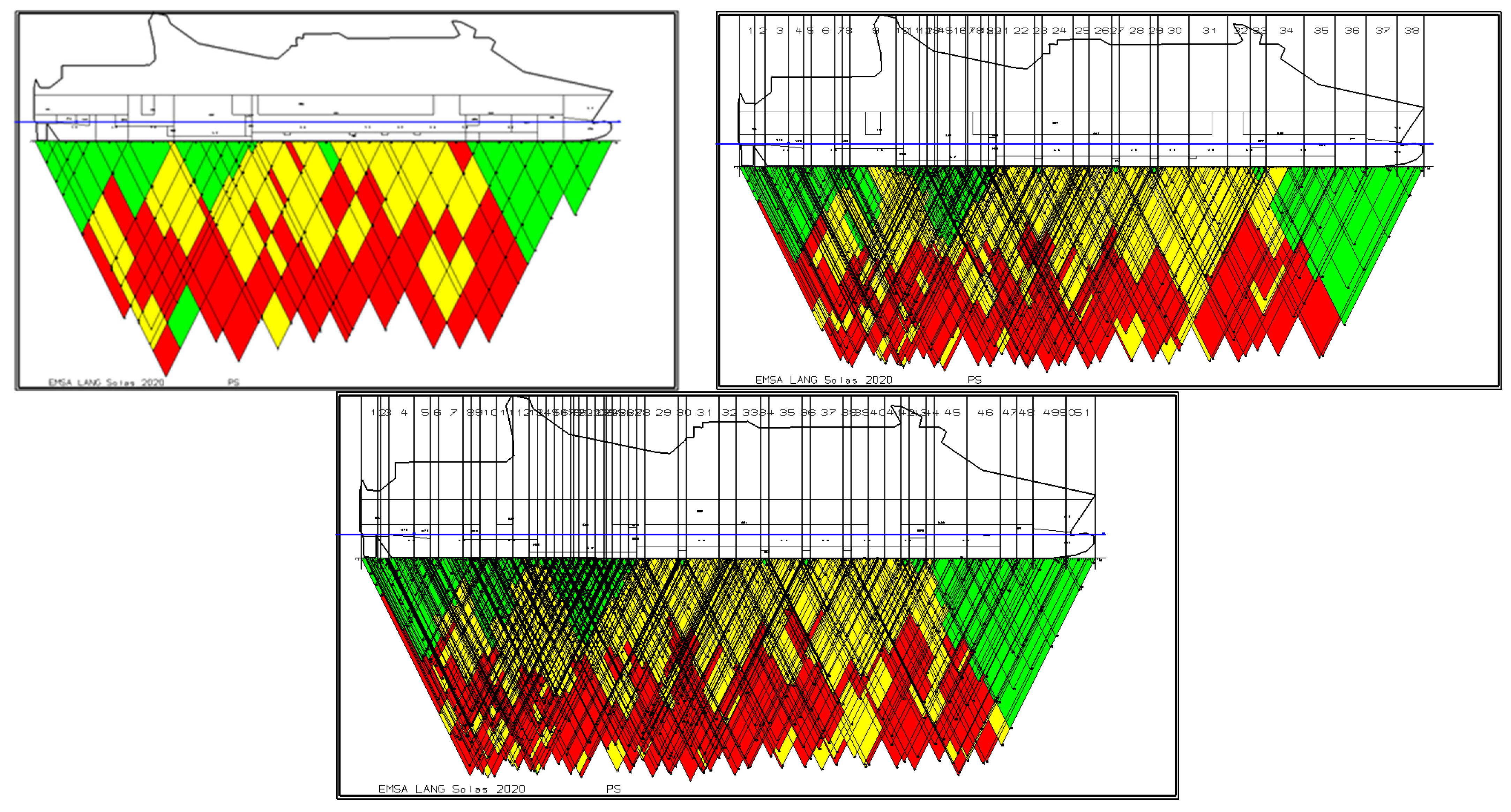
Figure 7 shows the graphical output of the damage stability simulations for three different configurations of damage zones. The picture on the top left shows the results if no damage zones have been defined. This is the setup of the classical Monte Carlo simulation method, but with the realization of the full extent damage cases. Each full extent damage case has a certain number of subcases. If the majority of these subcases is survived, the damage triangle is plotted in green, and if the majority is not survived, the triangle is red. All others are plotted in yellow. In this context, “majority” means the computation of an average Si,av for all damage cases of that group. The limit values can be set by the user, and the defaults which are also used in the following figures are Si,av > 0.85 for a green triangle and Si,av < 0.3 for a red triangle.
The realization without damage zones results in a total number of full extent cases of 228 and a total number of damage cases of 1776. In the top left picture of Figure 7, damage triangles can be seen. As the computation was without zones, these triangles correspond to the flooded lengths of each damage case as automatically computed by our algorithm.
In the top right picture, we have selected a damage zone setup with a damage zone at each transverse WTB of every compartment. This setup was determined automatically from the given compartmentation by a simple algorithm which searches for the x-Position of all transversal bulkheads of all compartments. This setup results in 38 damage zones. Now we obtain 453 full extent cases and 4995 damage cases. The obtained cases are exactly identical with the 1776 basic cases, but they are distributed over the defined damage zones. Other than in the realization without zones where the length of each triangle represented the flooded length, the length of each triangle now represents the individual damage length, mapped to the minimum or maximum x-value of the zone definition. The computed index is of course exactly the same as for the case without damage zones.
In Figure 7, bottom, we have repeated the calculation with a damage zone setup where we have positioned a damage zone at each transversal WTB of each space of a compartment. This setup was determined automatically from the given compartmentation by a simple algorithm which searches for the x-Position of all transversal bulkheads of all spaces of all compartments. This setup represents the finest reasonable subdivision into damage zones (51 damage zones), and at the same time we do now obtain the maximum number of damage cases. This results in 758 full extent damage cases and a total number of 7880 damage cases. The output is shown in Figure 7, bottom. This setup automatically solves the problem shown above for the steering gear compartment.
The advantage is that these two damage zone setups can be generated automatically without further user input from the compartmentation. However, the setup can be interactively modified by the user if found necessary. Additionally, it is well possible to use different zone setups for portside and starboard side damages. As shown above, the damage zone setup has no impact on the computational time and on the computed indices. It triggers only the number of damage cases and the splitting of Pi into pi and the related ri and vi probabilities.
If the automatically generated space based damage zone setup is used, the obtained output delivers exactly the same output as obtained from a conventional computation if the same zone setup is used, and therefore, it can be used for the generation of the statutory approval documents. This is because it automatically solves all the problems which have been addressed in this paper. However, this setup might lead to damage cases which exceed the storage capacity of conventional damage stability calculation programs, because not all of them can handle, e.g., 20 zone damages. Therefore, the user has the possibility to limit the maximum number of damage zones per damage case or he can alternatively modify the zone setup, if appropriate. For the user, the recommended procedure is furthermore quite straight forward; during the initial design, the method should be used as before without adding damage zones to the problem. Then, the compartmentation and the limiting stability curves can be optimized to meet the prescribed required index. If approval documents shall be generated, any user defined zone setup can be added, and the computation can simply be repeated. The output contains exactly the same information as obtained from a conventional damage stability computation and can consequently be submitted for approval. This development extends the Monte Carlo simulation principle now over the whole ship design process from basic design to delivery.
7. Operational Damage Stability
In the context of this section, operational damage stability is understood as the handling of the damage stability requirements during ship operation. In this regime, damage stability is accounted for as follows according to the SOLAS regulations. The attained index A is cumulated from the three indices on full, partial and light service draft. If the attained index A is larger than the required index R, the damage stability requirement is fulfilled, and the results are documented in the stability booklet as GM-Required curves. The ship must always be operated with a GM that is larger than the required GM, where in between values have to be interpolated. For the reference ship EMSA 2, the results of the damage stability calculation are summarized in the following table.
If the actual GM of the ship of a particular loading condition is larger than the limiting GMs, then damage stability is seen as fulfilled. Consequently, the damage stability limits of the ship strongly depend on the selection of the three drafts and their GMs. As there is only one equation (R = A), but three degrees of freedom (the three GMs), there is an infinite number of possible GM-required curves.
As a matter of fact, there are several possibilities to deal with damage stability during the operation of the ship. For example, the stability standard of the German Navy BV 1033 [16] explicitly requires that each loading condition must be analyzed in situ with respect to damage stability before the vessel is allowed to leave port. This means that the relevant damage stability procedures and requirements are in this context applied to a real loading condition. First of all, this means that the loading condition to be analyzed may have some tanks (bunkers, ballast) which are actually filled. The stability standard of the German Navy now requires a fluid exchange, which means that any damage tank is emptied before it is filled again with flood water. Further, all tanks which are partly filled (and are not damaged) must be treated by fluid shifting moments. This is a substantial difference compared to the SOLAS standard. Further, the cargo spaces are filled with a clearly specified cargo (volume, weight, and distribution), which means that realistic permeabilities for these compartments can be calculated.
If we make use of the Monte Carlo-simulation based procedure shown above, the damage stability computation requires practically no additional effort. This makes it attractive to use such kind of calculations also for the operation of the ship to analyze distinct loading conditions. The only change to the calculation code is now that prior to the stability calculation, all damaged tanks which have been filled must be emptied and the new mass and COG needs to be determined before the calculation of the righting levers is performed. As the required index is known from the damage stability calculation and documented in the stability booklet, it can be obtained for each loading condition. This principle is shown for the EMSA 2 RoPax in the following figure.
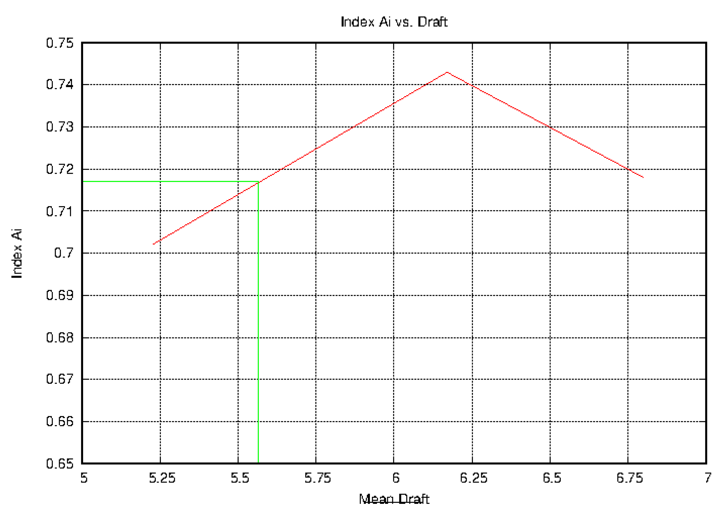
Figure 8 shows the index Ai as a function of the ship’s draft (see also Table 1). In the stability booklet of the ship, an equivalent figure is plotted showing the required GM-values. The stability booklet also contains a loading condition “Max Pax Departure” where the ship has a (mean) draft of 5.565 m (or 17,260 t displacement), which is shown in Figure 9. Following the damage stability requirements of the stability booklet, the ship must have a GM of 4.10 m to cope with the damage stability requirements. From Figure 8, the fact becomes obvious that for the 5.565 m draft, the index Ai can be interpolated as 0.717. This means that if we perform an operational damage stability calculation, this calculation must result in an index Ai for that particular loading condition of no less than 0.717 (means of port side and starboard side). For RoRo-passenger ships, it must also be verified that any Ai must be larger than 0.9 R. However, this must hold for all indices presented in Figure 8, and then it holds automatically for any interpolated index, too. In the framework of the research project DIGILECK (see acknowledgements) it was investigated under which boundary conditions this proposed procedure can be covered by the existing SOLAS explanatory notes.
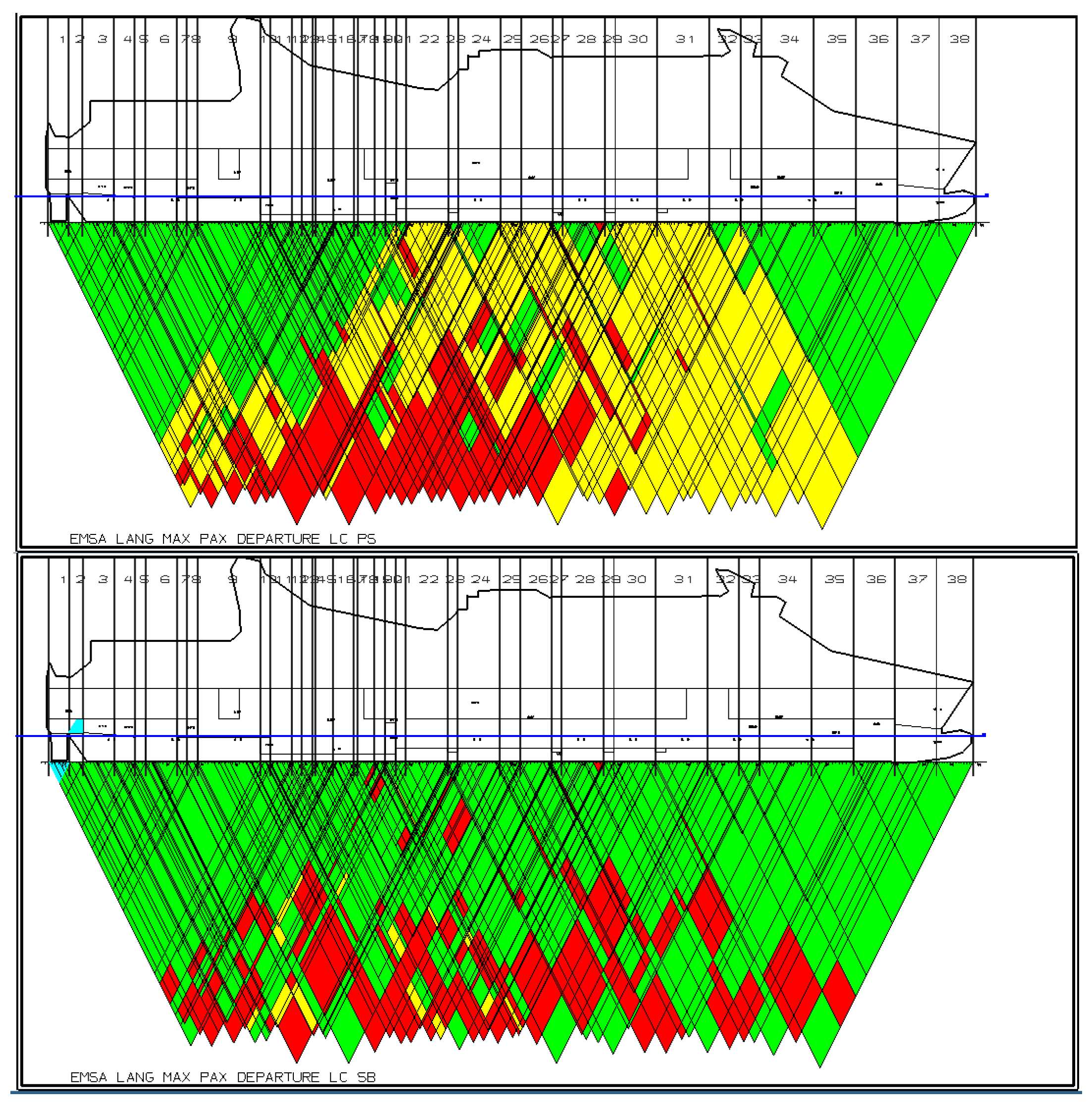
If we now perform this calculation, we obtain an Index Ai of 0.8067 on port side and 0.7935 on starboard side (see Figure 10), which is substantially more than 0.717. The difference is due to the effect of the fluid exchange of the tanks, as we did for the moment not alter the permeabilities of the RoRo-cargo holds. If it is sufficient to reach an index of 0.717, the GM can be lowered to 3.70 m, which is a substantial gain and significantly increases the flexibility of the ship, especially at the lower drafts. Additionally, it must again be pointed out that the calculation does not take any substantial effort.
8. Conclusions
A method was presented which extends the Monte Carlo principle for the computation of ship damage stability over the whole ship design process, including the automated generation of operational damage stability information. This demand requires the extension of the existing simulation method in two major points: At first, a second drawing of a modified cuboid with full penetration depth and maximum damage height results in so called full extent damage cases, which immediately allows to determine the probability pi. Secondly, the grouping of the resulting sub damage cases according to the penetration depths and damage heights allows the determination of vi and ri. This enables the simulation method to produce exactly the same output as the conventional calculation method, and the results can be approved by the classification society during the standard approval process. The extended method is in use by our industrial partners, and two damage stability calculations by the extended method have already passed the class approval.
The concept described for operational damage stability allows computation of damage stability for real loading conditions including the exchange of fluids, which results in a substantial gain in required GM. This concept significantly increases the flexibility of the ships especially on the lower drafts, which is most important for ships which carry project cargo on deck. However, before this operational damage stability concept can be used as a routine procedure during ship operation, it must further be investigated under which boundary condition the proposed concept is compatible with the SOLAS 2020 explanatory notes. Additionally, it might also be an interesting idea to shorten the computational time of the method further by applying the improved damage breach sampling process as suggested by Mauro and Vassalos [8].
Funding
This research was funded by the German Ministry for Economic Affairs and Energy, grant No. 03 SX 747 E.
Institutional Review Board Statement
Not applicable.
Informed Consent Statement
Not applicable.
Data Availability Statement
Not applicable.
Acknowledgments
The authors would like to thank the German Federal Ministry for Economic Affairs and Energy (BMWI) for funding this research work under the research contract DIGILECK 03 SX 474 E.
Conflicts of Interest
The author declares no conflict of interest.
References
- Krüger, S.; Dankowski, H. A Monte Carlo Based Simulation Method for Damage Stability Problems. In Proceedings of the OMAE, Glasgow, UK, 9–14 June 2019. [Google Scholar]
- Koelman, H. On the procedure for the determination of the probability of collision damage. Int. Shipbuild. Prog. 2005, 52, 129–148. [Google Scholar]
- Bulian, G.; Lindroth, D.; Ruponen, P.; Zaraphonitis, G. Probabilistic Assessment of Survivability in Case of Grounding: Development and Testing of a Direct Non-Zonal Approach. In Proceedings of the STAB, Glasgow, UK, 14–19 June 2015. [Google Scholar]
- Bulian, G.; Cardinale, M.; Dafermos, G.; Elioupoulou, E.; Francescutto, A.; Hamann, R.; Lindroth, D.; Luhmann, H.; Rupponen, P.; Zaraphonitits, G. Considering collision, bottom grounding and side grounding in a common non zonal framework. In Proceedings of the 17. STAB Workshop, Helsinki, Finland, 10–12 June 2019. [Google Scholar]
- Bulian, G.; Cardinale, M.; Dafermos, G.; Lindroth, D.; Ruponen, P.; Zaraphonitits, G. Probabilistic assessment of damaged survivability of passenger ships in case of grounding or contact. Ocean. Eng. 2020, 218, 107396. [Google Scholar] [CrossRef]
- Bulian, G.; Cardinale, M.; Francescutto, A.; Zaraphonitis, G. Complementing SOLAS damage ship stability framework with a probabilistic description for the extent of collision below the waterline. Ocean. Eng. 2019, 186, 106073. [Google Scholar] [CrossRef]
- Ruponen, P.; Lindroth, D.; Routi, A.L.; Aartovaara, M. Simulation- based analysis method for damage survivability of passenger ships. J. Ship Technol. Res. 2019, 66, 182–194. [Google Scholar] [CrossRef] [Green Version]
- Mauro, F.; Vassalos, D. The influence of damage breach sampling process on the direct assessment of ship survivability. Ocean. Eng. 2022, 250, 111008. [Google Scholar] [CrossRef]
- Kehren, F.I.; Krüger, S. Development of a Probabilistic Method for Damage Stability regarding Bottom Damages. In Proceedings of the PRADS, Houston, TX, USA; 2006. [Google Scholar]
- Dankowski, H.; Krüger, S. Progressive Flooding Assessment as an Extension of a Monte Carlo Based Damage Stability Method. In Proceedings of the PRADS, Changwon, Korea, 20–25 October 2013. [Google Scholar]
- Santos, T.A.; Soares, C.G. Monte Carlo Simulation of damaged ship survivability. J. Eng. Mar. Environ. 2005, 219, 25–35. [Google Scholar] [CrossRef]
- HARDER. Harmonization of Rules and Design Rationale; EU Contract No. CT-1998-00028. Final Technical Report; EU: Maastricht, The Netherlands, 1998. [Google Scholar]
- IMO. SOLAS 2020, Part B1; The International Maritime Organization: London, UK, 2020.
- Matsumoto, M.; Nishimura, T. Mersenne Twister: A 623-dimensionally equidistributed uniform pseudo random generator. ACM Trans. Model. Comput. Simul. 1998, 8, 3–30. [Google Scholar] [CrossRef]
- Valanto, P. Research for the Parameters of the Damage Stability Rules including the Calculation of Water on Deck of Ro-Ro Passenger Vessels, for the Amendment of the Directives 2003/25/EC and 98/18/EC; HSVA Report No. 1669; Hamburgische Schiffbau-Versuchs-Anstalt (HSVA): Hamburg, Germany, 2009. [Google Scholar]
- BAAINBw. Bauvorschrift für Wasserfahrzeuge der Bundeswehr Stability Regulation for Ships of the German Navy; BAAINBw: Koblenz, Germany, 2015. [Google Scholar]
Figure 1.
One and two compartment flooding.

Figure 2.
Principle of the Monte Carlo Method for damage stability problems. Here: Penetration depth for side damages.
Figure 2.
Principle of the Monte Carlo Method for damage stability problems. Here: Penetration depth for side damages.

Figure 3.
Simulation results for the EMSA2-RoPax. Black curve: Number of damage cases. Red curve: 5× Number of “fully” damaged cases.
Figure 3.
Simulation results for the EMSA2-RoPax. Black curve: Number of damage cases. Red curve: 5× Number of “fully” damaged cases.

Figure 4.
The steering gear compartment of the EMSA2-RoPax.

Figure 5.
Void Space 3 of the RoPax EMSA2.

Figure 6.
Two models of the EMSA2 RoPax.

Figure 7.
Damage stability output with three different damage zone realizations.

Figure 8.
Index Ai as a function of the draft for the EMSA2 RoPax.

Figure 9.
Loading condition Pax Departure for the EMSA-RoPax.

Figure 10.
Output of the operational damage stability calculation for ps (left) and stb (right). GM = 3.70 m.
Figure 10.
Output of the operational damage stability calculation for ps (left) and stb (right). GM = 3.70 m.


Table 1.
Damage stability results for the EMSA 2 RoPax [15].
Table 1.
Damage stability results for the EMSA 2 RoPax [15].
| Denomination | Draft A.P. | Draft F.P. | Displacement | GM | Index | Index | Index |
|---|---|---|---|---|---|---|---|
| [m] | [m] | [t] | [m] | PS | STB | Mean | |
| Light | 5.74 | 4.75 | 16,081 | 4.50 | 0.724 | 0.680 | 0.702 |
| Partial | 6.17 | 6.17 | 19,933 | 4.10 | 0.761 | 0.725 | 0.743 |
| Deepest | 6.80 | 6.80 | 22,875 | 4.10 | 0.735 | 0.700 | 0.718 |
Disclaimer/Publisher’s Note: The statements, opinions and data contained in all publications are solely those of the individual author(s) and contributor(s) and not of MDPI and/or the editor(s). MDPI and/or the editor(s) disclaim responsibility for any injury to people or property resulting from any ideas, methods, instructions or products referred to in the content. |
© 2022 by the author. Licensee MDPI, Basel, Switzerland. This article is an open access article distributed under the terms and conditions of the Creative Commons Attribution (CC BY) license (https://creativecommons.org/licenses/by/4.0/).
Share and Cite
MDPI and ACS Style
Krüger, S. Statutory and Operational Damage Stability by a Monte Carlo Based Approach. J. Mar. Sci. Eng. 2023, 11, 16. https://doi.org/10.3390/jmse11010016
AMA Style
Krüger S. Statutory and Operational Damage Stability by a Monte Carlo Based Approach. Journal of Marine Science and Engineering. 2023; 11(1):16. https://doi.org/10.3390/jmse11010016
Chicago/Turabian StyleKrüger, Stefan. 2023. "Statutory and Operational Damage Stability by a Monte Carlo Based Approach" Journal of Marine Science and Engineering 11, no. 1: 16. https://doi.org/10.3390/jmse11010016
Note that from the first issue of 2016, this journal uses article numbers instead of page numbers. See further details here.