Article

Simulating Ship Manoeuvrability with Artificial Neural Networks Trained by a Short Noisy Data Set

Centre for Marine Technology and Ocean Engineering (CENTEC), Instituto Superior Técnico, Universidade de Lisboa, Av. Rovisco Pais, 1049-001 Lisboa, Portugal
*
Author to whom correspondence should be addressed.
J. Mar. Sci. Eng. 2023, 11(1), 15; https://doi.org/10.3390/jmse11010015
Submission received: 14 November 2022 / Revised: 18 December 2022 / Accepted: 19 December 2022 / Published: 22 December 2022
(This article belongs to the Special Issue Maritime Autonomous Vessels)

Abstract

:
Artificial neural networks are applied to model the manoeuvrability characteristics of a ship based on empirical information acquired from experiments with a scaled model. This work aims to evaluate the performance of the proposed method of training the artificial neural network model even with a very small quantity of noisy data. The data used for the training consisted of zig-zag and circle manoeuvres carried out in agreement with the IMO standards. The wind effect is evident in some of the recorded experiments, creating additional disturbance to the fitting scheme. The method used for the training of the network is the Levenberg–Marquardt algorithm, and the results are compared with the scaled conjugate gradient method and the Bayesian regularization. The results obtained with the different methodologies show very suitable accuracy in the prediction of the referred manoeuvres.

1. Introduction

The prediction of ship dynamics in the seaway is complicated as it depends on the joint effect of the various environmental factors, independently of whether the interest is to predict the ship dynamics in straight trajectories or when performing manoeuvres.
Methods are available to determine manoeuvring trajectories from a given manoeuvring mathematical model. Several popular mathematical models for ship manoeuvrability have been widely applied, such as the Abkowitz model [1,2,3], the Manoeuvring Mathematical Group (MMG) model [4], the well-known Nomoto model [5], or even more detailed models proposed recently [6]. Reviews covering several elected issues associated with vessel mathematical models employed in ship manoeuvring, principally for simulation purposes, are presented in [7,8]. The need to have an accurate and fast prediction of ship responses is associated with ship manoeuvring, in particular, in decision support systems for ship handling or manoeuvring simulators led to the development of several empirical models [9].
The manoeuvring model’s parameters may be estimated using different methods, including different types of regressions when captive model tests are performed [10,11] or several system identification techniques, which typically are applied on free-running model tests or full-scale tests [12,13]. Various system identification methods for vessels are available, such as the ones presented in [14,15,16,17,18]. When a model has parameters already identified, then it can be used to simulate the ship trajectories [19].
Artificial intelligence methods have been used to model different types of responses [20,21]. Neural networks have been used to predict manoeuvring capabilities [22]. A ship’s minimum time manoeuvring system based on artificial neural networks (ANNs) and a nonlinear model predictive compensator was presented in [23], allowing the user to execute the optimization for any desired set of equality and non-equality constraints. The work presented in [24] is focused on getting optimized ship trajectories in narrow waterways under wind disturbances considering time as an objective function, i.e., the ship tends to sail by taking the optimized rudder output for minimum time manoeuvre. Later, in [25], the same authors studied the application of an ANN controller for ship course-changing manoeuvres. In [26], a method that uses genetic algorithms to simultaneously optimize the number and weights of backpropagation neural network neurons to predict the ship’s trajectory is studied.
Another ANN class that has been used to model ship dynamics is the Recurrent Neural Network (RNN). In an RNN, the connections between nodes form a directed or undirected graph along a temporal sequence, allowing it to exhibit a temporal dynamic behaviour. RNNs have been used in different maritime applications, such as the study presented in [27] that presents the use of an RNN for the prediction of the propulsion power of a vessel. In [28], a real-time ship vertical acceleration prediction algorithm based on the long short-term memory (LSTM) and gated recurrent units (GRU) models of an RNN is proposed. In [22], an RNN is used to model the surface ships’ manoeuvrability characteristics. In [22], an RNN with four inputs, one hidden layer, and two outputs was used to learn the manoeuvring model of a ship from data generated through simulations. Inputs to the model are the commands of rudder angle and ship’s speed, in addition to the recursive outputs sway and yaw velocities. The outputs of the system were the rate of sway and yaw at the current time instant.
A posteriori, the model presented in [22] was used to analyse the potential of ANNs in ship simulation when the training data are corrupted with noise, as is usually the case in full-scale tests [29]. An RNN to simulate catamaran manoeuvres was presented as a different methodology from the conventional approach of developing manoeuvring mathematical models [30]. The work presented here aims to assess the performance of ship manoeuvrability models developed by applying RNNs trained with a low quantity of noisy data from zig-zag and circle experiments carried out in agreement with the IMO standards [31].
Later, deep structured learning architectures such as long short-term memory (LSTM) networks, which are a type of RNN able to process not only single data points but also entire sequences of data, have been applied to the dynamic model identification [32]. Other methods are also available and have been used in specific data-based motion predictor applications such as support vector machines (SVMs) [16,33,34,35], deep learning, or auto-regressive (AR) methods. On the other side, there exist model-based predictors such as dynamic models [19]. Several applications have been developed in the scope of the improvement of manoeuvring performance.
The main objective of the development of the RNN model is to obtain an alternative to the usual manoeuvring simulators that use traditional mathematical models, which are a function of the hydrodynamic forces and moment derivatives. These values are normally achieved through captive experiments performed with models in tanks. This procedure is time-consuming and costly, requiring exclusive use of a large specialized, purpose-built facility. Another possibility is to use the trajectories of small or even large self-propelled models to train neural networks or to identify the parameters of the traditional mathematical models. Furthermore, this is one of the valid methods that can be used in the design stage of a ship.
The alternative RNN model presented in this paper represents an implicit mathematical model for ships in which time histories of manoeuvring motions are previously known. The main advantage of the RNN consists in that the parameters used for the training are easily obtained from full-scale trials of existing ships or self-propulsion tests of models. RNNs can handle noisy data because they can generalize after training on noisy data instead of merely memorizing the noise.
The RNN model used in this paper for the manoeuvring simulation is based on the one used in [31], but it takes much less data for the network training using the methods presented in a previous study, which handled only simulated data [36], while here real measurements are used. The RNNs studied have the advantage of having very few parameters making them very fast to train. The performance of the network is analysed regarding the limited data set used for training. RNNs are autonomous but highly susceptible to errors. If the data set is small enough not to be inclusive, biased predictions may come from a biased training set.
In recent years, ANNs have been effectively used in an extensive range of maritime applications. The vessel dynamics may also be considered as a black box and modelled using a proper tool. ANNs have been used for the problem of parameter estimation in [37], where the weights of the network correspond to the parameters of the Nomoto model. The network learns these parameters from data acquired experimentally. One more application, presented in [38], uses a feedforward ANN to learn the behaviour of the nonlinear terms of the manoeuvring model from data obtained through numerical simulations. This ANN is then used in simulations to replace the calculation of the nonlinear terms. In [39], RNNs were used as manoeuvring simulation tools. Inputs to the simulation, cast in the form of forces and moments, were redefined and extended in a manner that accurately captures the physics of ship motion.
In the present case study, the main innovation is to train the network using a different methodology, the Levenberg–Marquardt algorithm, instead of the backpropagation method. This methodology is used to solve nonlinear least squares problems, and it is a combination of two other methods: gradient descent and Gauss–Newton. As there are two possible options for the algorithm’s direction at each iteration, the Levenberg–Marquardt is more robust than the Gauss–Newton. As an advantage, it shows to be faster to converge than either the Gauss–Newton or gradient descent. In addition, it can handle models with multiple free parameters that are not precisely known. If the initial guess is far from the mark, the algorithm can still find an optimal solution. In this paper, the results obtained with the Levenberg–Marquardt algorithm are compared with the ones obtained with the training performed with two different methods: the scaled conjugate gradient method and Bayesian regularization. The Levenverg–Marquardt algorithm allowed training the system with a relatively short training time series.
Section 2 carries out the description of the manoeuvring tests, along with a summary of the acquired results and the pre-processing steps executed before using them for training and testing. Section 3 reports the configuration and training method of the presented RNN model. Section 4 presents the results acquired with the proposed model. Lastly, Section 5 outlines and analyses the results, comparing them with values attained with models being used for analogous assignments under identical situations.

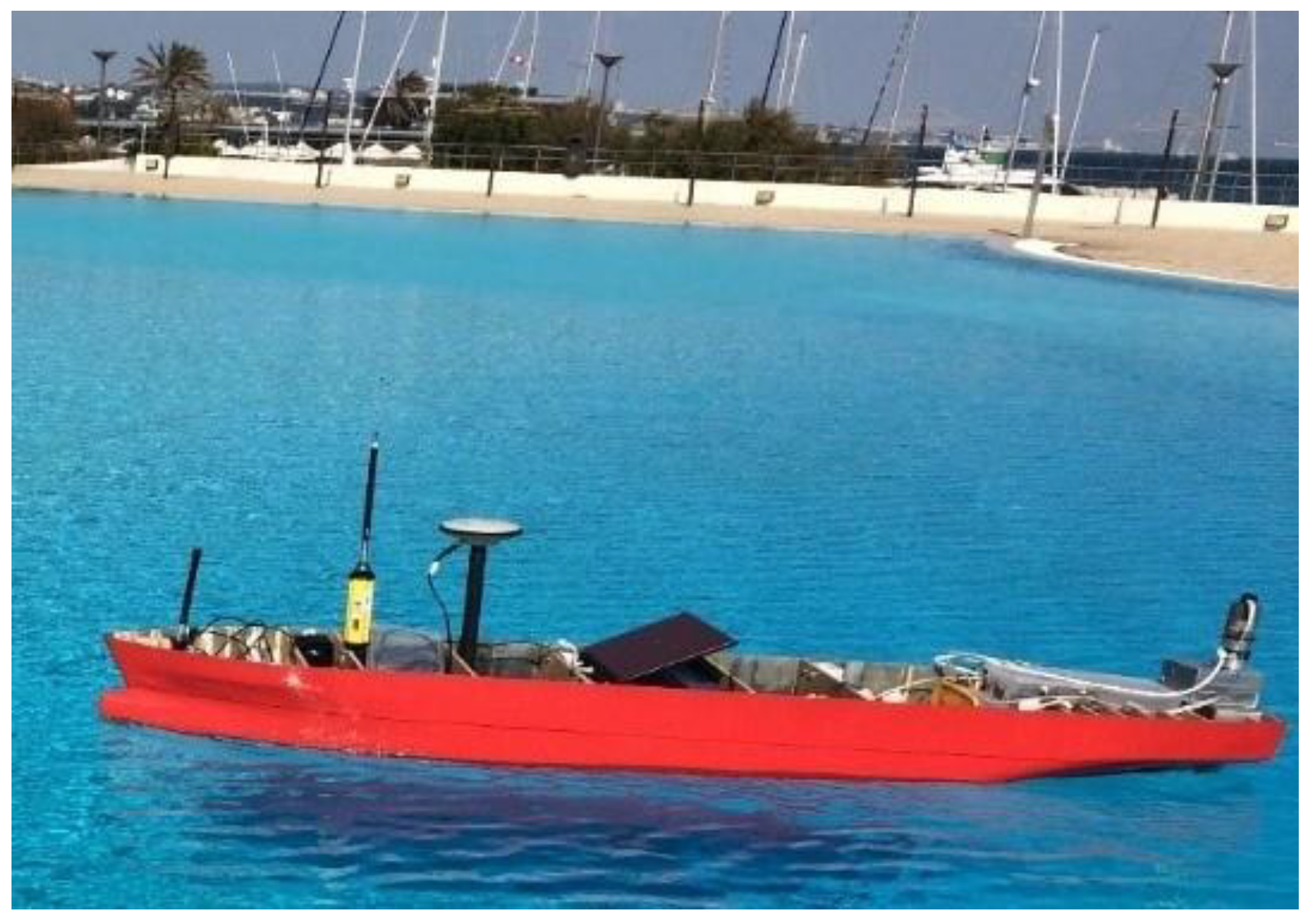
2. Description of the Manoeuvring Tests

The manoeuvring experiments executed to collect the data used in this article paper are presented in [40,41]. The experiments were conducted on the “Piscina Oceaˆnica de Oeiras”, Portugal, with the chemical tanker ship model in March 2016. This swimming pool has a length of 50 m and a breadth of 30 m. The model is a scaled model of a chemical tanker built at the “Estaleiros Navais de Viana do Castelo”, Portugal.
The scaled (1/65.7) model of the chemical tanker is shown afloat in Figure 1, and its main dimensions are stated in Table 1, together with the ones of the real ship. The vehicle is built from single-skin glass-reinforced polyester with plywood framings, and its design speed is 0.98 m/s.
The hardware architecture comprises all the sensors and actuators that are used in the real-time navigation and control platform. The hardware structure is further split into a command and monitoring unit (CMU) and a communication and control unit (CCU).
The main goal of the shore-based CMU is to assist in the manual and autonomous control of the vehicle by providing a human–machine interface (HMI). The CMU mostly consists of various instrumentations: laptop, global positioning system (GPS) unit, industrial Wi-Fi unit, compact-RIO, main AC power supply unit, DC power supply unit, and an anemometer to measure the relative wind speed and direction.
The main goal of the onboard CCU is to execute real-time control algorithms that are related to the course and speed controls of the model. The CCU comprises the following instrumentations: laptop, CompacRIO units, industrial Ethernet switch (IES), GPS unit, inertial measurement system (IMS) (capable of measuring the 3-axis angles of heading, roll, and pitch, the 3-axis angular velocities of heading, roll, and 3-axis linear accelerations of surge, sway, and heave), industrial Wi-Fi unit, DC motors with encoders able to take the measurements of the 3-axis angles of heading, roll, and pitch, the 3-axis angular velocities of heading, roll, and 3-axis linear accelerations of surge, sway, and heave, position sensor, fibre-optic gyrocompass, laptop computer, batteries, and fuse units.
Measurement and registration of the kinematical parameters listed in Table 2 were envisaged, and all parameters indicated in the table were measured during the tests. The uncertainty estimates are approximate and were obtained from the instruments’ documentation.
The GPS unit generates instantaneous ship coordinates in terms of latitude φ and longitude λ. These are transformed to the standard Cartesian earth coordinates of the ship’s origin ξC and ηC for the manoeuvre’s starting point (Figure 2):
ξ C = κ ( ϕ ϕ 0 )
η C = κ ( λ λ 0 ) c o s ϕ 0
The subscript ‘0’ denotes the initial values of the corresponding variables, and κ is the conversion coefficient from minutes to meters equal to 1852 m/min. In Figure 2 β is the drift angle, χ is the course angle provided by the GPS, ψ is the heading angle, δR is the rudder angle, r is the yaw rate, V is the speed of the ship, VA is the relative wind speed, βA is the wind drift angle, and χA is the wind course angle.
After this initial transformation, the coordinate ξ is assumed to be measured along the true meridian while η is along the parallel. However, when analysing the trajectories, the coordinates are transformed further so that the origin of the earth axes matches the ship’s position at the start of a manoeuvre, and the ξ-axis is directed along the approach path.
Altogether, six test runs with the model are used for the training of the network, namely, four zigzags and two circles. Table 3 presents a summary of the data collected. In total, 5229 data points are provided (2348 from turnings and 2881 from zig-zag tests). Since the forward speed was not recorded, because the GPS used to track the model position only feedbacks the position and time, it was replaced in the model with the revolutions per minute (RPM) values. In this case, the orders are rudder angle and RPMs for certain sailing conditions. Increasing the RPM value increased the model forward speed, and decreasing the RPM decreased the model speed. RPM means the rotations of the propeller, which is directly related to the speed imparted to the ship. Changing RPM changes the speed.
The analysis of the experimental data suggests that the trajectories have been modified by the effect of wind as the circles are not concentric and show a drift, which would be the effect of wind and current [42].

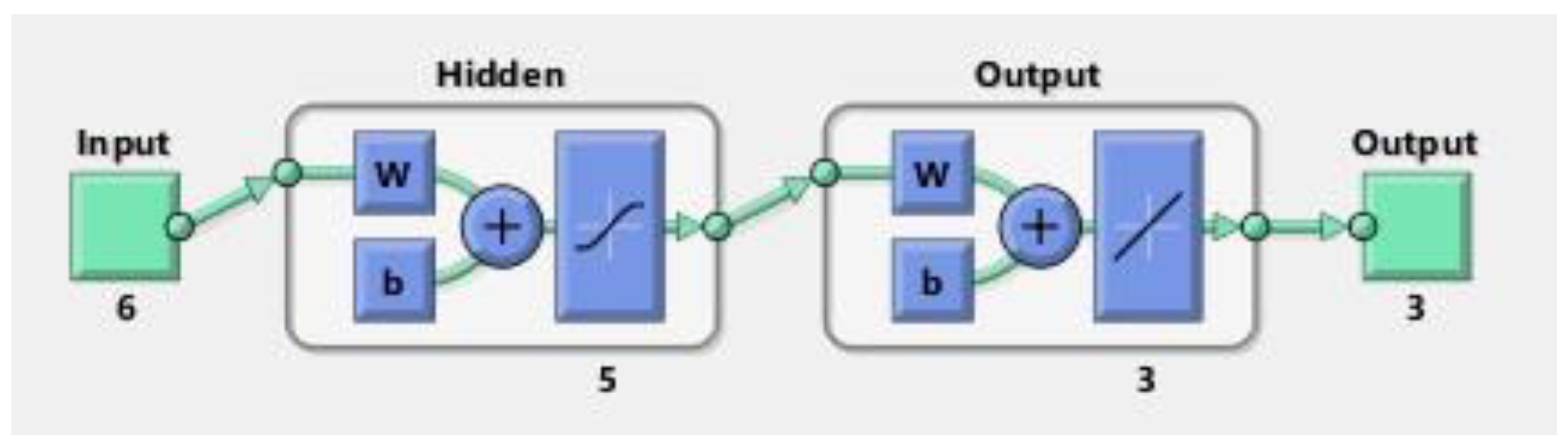
3. Neural Network Training

The model used has the following six inputs:
  • Rudder angle θ(k);
  • RPM(k);
  • Sway velocity at previous time step v(k − 1);
  • Heading angle at previous time step ψ (k − 1);
  • x position at previous time step x(k − 1);
  • y position at previous time step y(k − 1);
and three outputs:
  • Heading angle at current time step ψ (k);
  • x position at current time step x(k);
  • y position at current time step y(k).
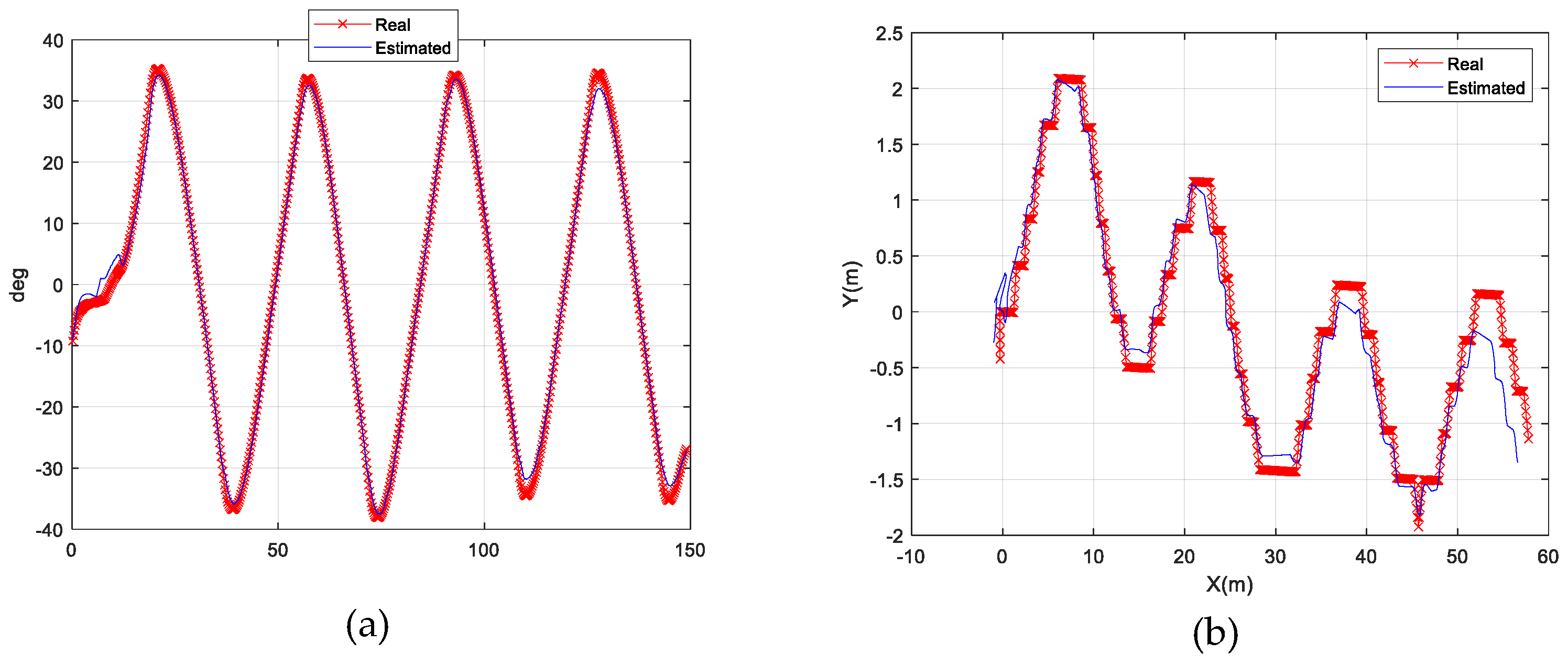
Connecting inputs and outputs is a single hidden layer with five neurons. A sigmoid-based activation function is applied to every neuron in the hidden layer, creating a structure with the capability to provide smooth results. The function is given by:
f ( x i ) = e x i e x i + 1
where x is the input of neuron i.
It can be seen in Table 3 that the wind conditions during the zig-zag tests are very similar but different from the wind conditions of the circles. Due to this difference in wind conditions, it is not appropriate to train a model on zig-zag data and validate it on circle data or vice versa. Two separate models are trained, one for each type of test. The training data points are all concatenated into two arrays, one for zig-zag tests and another one for circle tests. Each of these two arrays was then split according to the following proportions:
80% of the data points used for training;
10% of the data points used for validation;
10% of the data points used for testing.
Usually, multilayer perceptrons (MLPs) are trained with the backpropagation technique, but in this work, the damped least-squares method, also known as the Levenberg–Marquardt algorithm, is employed, as well as the scaled conjugate gradient and Bayesian regularization methods for comparison.
Although backpropagation is a gradient descent technique, the Levenberg–Marquardt algorithmic rule is deduced from Newton’s procedure that was defined to minimize functions that are additions of squares of nonlinear functions [43], as the configuration below:
E = 1 2 k ( e k ) 2 = 1 2 e 2
where ek is the error in the kth exemplar and e is the vector of the elements ek. If the discrepancy between the preceding weight vector and the current one is small, the vector of the errors can be approximated to the first order using Taylor series expansion:
e ( j + 1 ) = e ( j ) + e k w i ( w ( j + 1 ) w ( j ) )
Therefore, the error function can be displayed as:
E = 1 2 e ( j ) + e k w i ( w ( j + 1 ) w ( j ) ) 2
Minimizing the error function in regard to the current weight vector:
w ( j + 1 ) = w ( j ) ( J T J ) 1 J T e ( j )
where ( J ) k i = e k w i is the Jacobian matrix.
The Hessian matrix for the sum-of-square error function is expressed by:
( H ) i j = 2 E w i w j = { ( e k w i ) ( e k w i ) + e k 2 e k w i w j }
Neglecting the second term in (8), the matrix can be updated as:
H = JTJ
The weights modification needs to take the inverse of the Hessian. The matrix is fairly uncomplicated to compute since it is grounded on first-order partial derivatives in regard to the network weights that are easily managed by the training algorithm. Although the updating equation is used repetitively to reduce the error function, this may generate a large step size, which could refute the linear approximation on which the equation is based. In the Levenberg–Marquardt algorithm, the error function is reduced to a minimum while the step size is remained low intending to guarantee the effectiveness of the linear approximation. This minimization is obtained through a modified error function of the following configuration:
E = 1 2 e ( j ) + e k w i ( w ( j + 1 ) w ( j ) ) 2 + λ w ( j + 1 ) w ( j ) 2
where λ is a parameter governing the step size. Reducing the modified error to a minimum with regard to w(j + 1):
w ( j + 1 ) = w ( j ) ( J T J + λ I ) 1 J T e ( j )
When λ is null, (11) simply describes Newton’s method, using the approximation to the Hessian matrix. Once λ is large, the formula converts to the steepest descent with a small step size. Newton’s method is faster and more accurate when it is close to an error minimum; thus, the objective is to switch to Newton’s method promptly. Consequently, λ is reduced after every successful step (reduction in performance function) and is increased just in case a tentative step would increase the performance function. Thus, the performance function is decreased every time at all procedure iterations.
In this study, a single-hidden-layer MLP network is applied in MatLab and trained using the Levenberg–Marquardt algorithm. For the training mechanism, four input variables and two output variables were employed, as aforementioned. The quantity of hidden neurons of 5 was chosen after a methodical examination of the system convergence and generalization ability.
A diagram of the designed framework is shown in Figure 3. Investigations concerning the training performance of different variants of the Backpropagation algorithms establish that the Levenberg–Marquardt algorithm is the fastest to converge. In addition, comparisons of predictions made by the different neural networks reveal that the neural network trained using the Levenberg–Marquardt algorithm gives the most accurate predictions. Results supporting these affirmations can be found in [44]. The fast convergence teamed with suitable predictive quality reported in the bibliography makes the Levenberg–Marquardt algorithm the primary suitable choice for training the neural network for the application developed in this work.
In summarizing, in this study, a single-hidden-layer MLP network is applied in MatLab and trained by making use of the three different algorithms for comparison: the Levenberg–Marquardt, the scaled conjugate gradient, and Bayesian regularization methods. For the training mechanism, six input variables and three output variables are employed, as aforementioned. In this case, the rule-of-thumb method to determine the number of neurons to use in the hidden layer was based on the number of hidden neurons that should be between the size of the input layer and the size of the output layer. Different trials were performed with a different number of neurons between 3 and 6 in the hidden layer taken for each trial to determine the sensitivity of the neural network to these number of hidden neurons on the training performance. Then, 5 was chosen for the number of neurons in the hidden layer. These results are omitted from the text because they do not present interesting information.

4. Results

Figure 4a, Figure 5a, Figure 6a and Figure 7a show the predicted and experimental heading angle for data sets ZigZag1 to 4, and Figure 4b, Figure 5b, Figure 6b and Figure 7b show the respective predicted and experimental trajectories. The parameter used to assess the model error in zig-zag tests is the average heading error, and the results are based on the entire data set (All) using the scaled conjugate gradient method.
The correlation coefficient r is calculated to control how well the system output fits the desired output. The correlation coefficient between a network output x and the desired output d is stated by:
r = i ( x i x ¯ ) ( d i d ¯ ) N i ( d i d ¯ ) 2 N i ( x i x ¯ ) 2 N
where N is the number of observations.
The best r values acquired for the approximation of the heading angle for the zig-zag manoeuvres are registered in Table 4 for the training, validation, and test subsets, as well as for the entire data set (all) for the three different methods considered.
The predictions for the zig-zag manoeuvres are very suitable, as can be seen in Figure 4, Figure 5, Figure 6 and Figure 7 and in the results listed in Table 4. It can be noticed that the predictions in almost all the runs are very similar, mainly because all the trials were performed under the same environmental conditions. From the obtained results presented in Table 4, it can be seen that it is possible to predict the heading angle with very suitable accuracy for all three studied methods.
In Figure 4b, it can be seen that for x values larger than 50 m, there is a significant deviation in the predicted value. This can be explained from the wind velocity plot for this trial, presented in Figure 8, where it can be seen that around 400 s of the trajectory, the wind speed decreases, which causes a slowdown in the trajectory. For this reason, the neural network that had learned the trajectory of the previous instants had the tendency to continue with the same progress on the y-axis.
For assessing the performance of the model in circle tests, the tactical diameter is of interest. The tactical diameter is defined as the distance between two points whose heading differs by 180°. Figure 9 and Figure 10 show the predicted and experimental trajectories for data sets Turning 1 and Turning 2 using the Lavenberg–Marquardt method.
The best r results obtained for the positions x and y approximations for the circle manoeuvres are registered in Table 5 and Table 6, respectively. The predictions for the circle manoeuvres are also very suitable, as can be seen from Figure 9 and Figure 10 and through the results listed in Table 5, despite only having two data sets available, with the only difference between them being the rudder angle. The graphical results of Figure 9 and Figure 10 indicate the evaluation of the predictive accuracy of the model. The plots show how well the model predicts and fit the values of the variables obtained in the real experiments. The plots are computed by using the “all” data results.
Again, from the obtained results presented in Table 5 and Table 6, it can be seen that it is possible to predict the x and y positions with very suitable accuracy for all three studied methods.
Since neural networks are expected to be suitable interpolators, it can be assessed if the network generalizes well by giving input rudder angles between 20° and 26° because the circle tests were performed for these two values of rudder commands. Since no data are available, it is not possible to quantify the error of these simulations.

5. Conclusions

A method based on ANNs has been implemented to predict the heading angle and trajectories of a model ship from the output rudder angle command, the RPM of the propulsion shaft, the measurements of sway velocity, heading angle, and x and y positions at the previous time step. The training results were presented for the Levenberg–Marquardt algorithm and compared with the scaled conjugate gradient and Bayesian regularization methods. The information used to train and validate the system was acquired through manoeuvring tests with a chemical tanker model ship.
The obtained neural network system is suitable for producing precise approximations of the mentioned variables, showing that it is possible to obtain suitable results with an ANN trained using only five hidden neurons. The main feature of this study is to demonstrate that the ANN is able to learn even from a short and noisy data set. In addition, the method can be useful for predicting manoeuvring capabilities in the design stage of a ship. In future work, it is expected to be applied to different types of ships.

Author Contributions

Funding acquisition, C.G.S.; formal analysis, L.M.; writing—original draft, L.M.; writing—review and editing, C.G.S.; methodology, L.M.; software, L.M.; supervision, C.G.S. All authors have read and agreed to the published version of the manuscript.

Funding

The research was performed within the NAVAD project “Simulation of manoeuvrability of ships in adverse weather conditions”, which is co-funded by the European Regional Development Fund (Fundo Europeu de Desenvolvimento Regional—FEDER) and by the Portuguese Foundation for Science and Technology (Fundação para a Ciência e a Tecnologia—FCT) under contract 02/SAICT/032037/2017. This work contributes to the Strategic Research Plan of the Centre for Marine Technology and Ocean Engineering (CENTEC), which is financed by the Portuguese Foundation for Science and Technology (Fundação para a Ciência e Tecnologia—FCT) under contract UIDB/UIDP/00134/2020.

Institutional Review Board Statement

Not applicable.

Informed Consent Statement

Not applicable.

Data Availability Statement

Not applicable.

Conflicts of Interest

The authors declare no conflict of interest.

Abbreviations

ANNArtificial neural network
RNNRecursive neural network
MMGManoeuvring Mathematical Group
LSTMLong short-term memory
SVMSupport vector machine
CMUCommand and monitoring unit
CCUCommunication and control unit
HMIHuman–machine interface
IESIndustrial Ethernet switch
MLPMultilayer perceptron
RPMRevolutions per minute

References

  1. Crane, C.L.; Eda, H.; Landsburg, A.C. Controllability. In Principles of Naval Architecture; Lewis, E.V., Ed.; SNAME: Jersey City, NJ, USA, 1989; Volume 3, pp. 191–422. [Google Scholar]
  2. Abkowitz, M.A. Measurement of hydrodynamic characteristics from ship maneuvring trials by system identification. SNAME Trans. 1980, 88, 283–318. [Google Scholar]
  3. Abkowitz, M.A. Measurements of ship resistance, powering and maneuvering coefficients from simple trials during a regular voyage. Trans. SNAME 1988, 96, 97–128. [Google Scholar]
  4. Ogawa, A.; Kasai, H. On the mathematical model of manoeuvring motion of ships. Int. Shipbuild. Prog. 1978, 25, 306–319. [Google Scholar] [CrossRef]
  5. Nomoto, K.; Taguchi, T.; Honda, K.; Hirano, S. On the steering qualities of ships. Int. Shipbuild. Prog. 1957, 4, 354–370. [Google Scholar] [CrossRef]
  6. Sutulo, S.; Guedes Soares, C. Development of a core mathematical model for arbitrary manoeuvres of a shuttle tanker. Appl. Ocean. Res. 2015, 51, 293–308. [Google Scholar] [CrossRef]
  7. Sutulo, S.; Guedes Soares, C. Mathematical models for simulation of manoeuvring performance of ships. In Marine Technology and Engineering; Guedes Soares, C., Garbatov, Y., Fonseca, N., Teixeira, A.P., Eds.; Taylor & Francis Group: London, UK, 2011; pp. 661–698. [Google Scholar]
  8. Sutulo, S.; Guedes Soares, C. Review on ship manoeuvrability criteria and standards. J. Mar. Sci. Eng. 2021, 9, 904. [Google Scholar] [CrossRef]
  9. Sutulo, S.; Guedes Soares, C. On the application of empiric methods for prediction of ship manoeuvring properties and associated uncertainties. Ocean Eng. 2019, 186, 106111. [Google Scholar] [CrossRef]
  10. Sutulo, S.; Guedes Soares, C. Synthesis of experimental designs of manoeuvring captive-model tests with large number of factors. J. Mar. Sci. Technol. 2004, 9, 32–42. [Google Scholar] [CrossRef]
  11. Sutulo, S.; Guedes Soares, C. Development of a multifactor regression model of ship manoeuvring forces based on optimized captive-model tests. J. Ship Res. 2006, 50, 311–333. [Google Scholar] [CrossRef]
  12. Guedes Soares, C.; Sutulo, S.; Francisco, R.A.; Santos, F.M.; Moreira, L. Full-scale measurements of the manoeuvring capabilities of a catamaran. In Proceedings of the International Conference on Hydrodynamics of High Speed Craft, London, UK, 24–25 November 1999; RINA: London, UK, 1999; pp. 1–12. [Google Scholar]
  13. Guedes Soares, C.; Francisco, R.A.; Moreira, L.; Laranjinha, M. Full-scale measurements of the manoeuvering capabilities of fast patrol vessels, Argos class. Mar. Technol. 2004, 41, 7–16. [Google Scholar]
  14. Sutulo, S.; Guedes Soares, C. An algorithm for offline identification of ship manoeuvring mathematical models after free-running tests. Ocean Eng. 2014, 79, 10–25. [Google Scholar] [CrossRef]
  15. Perera, L.P.; Oliveira, P.; Guedes Soares, C. System identification of vessel steering with unstructured uncertainties by persistent excitation maneuvers. IEEE J. Ocean Eng. 2016, 41, 515–528. [Google Scholar] [CrossRef]
  16. Xu, H.; Hinostroza, M.A.; Hassani, V.; Guedes Soares, C. Real-time parameter estimation of nonlinear vessel steering model using support vector machine. J. Offshore Mech. Arct. Eng. 2019, 141, 061606. [Google Scholar] [CrossRef] [Green Version]
  17. Wang, Z.; Zou, Z.; Guedes Soares, C. Identification of ship manoeuvring motion based on nu-support vector machine. Ocean Eng. 2019, 183, 270–281. [Google Scholar] [CrossRef]
  18. Costa, A.C.; Xu, H.T.; Guedes Soares, C. Robust parameter estimation of an empirical manoeuvring model using free-running model test. J. Marit. Sci. Eng. 2021, 9, 1302. [Google Scholar] [CrossRef]
  19. Sutulo, S.; Moreira, L.; Guedes Soares, C. Mathematical models for ship path prediction in manoeuvring simulation systems. Ocean Eng. 2002, 29, 1–19. [Google Scholar] [CrossRef]
  20. Xu, Y.; Liu, X.; Cao, X.; Huang, C.; Liu, E.; Qian, S.; Liu, X.; Wu, Y.; Dong, F.; Qiu, C.-W.; et al. Artificial intelligence: A powerful paradigm for scientific research. Innovation 2021, 2, 100179. [Google Scholar] [CrossRef]
  21. Atluri, G.; Karpatne, A.; Kumar, V. Spatio-temporal data mining: A survey of problems and methods. ACM Comput. Surv. 2017, 51, 1–41. [Google Scholar] [CrossRef]
  22. Moreira, L.; Guedes Soares, C. Dynamic model of manoeuvrability using recursive neural networks. Ocean Eng. 2003, 30, 1669–1697. [Google Scholar] [CrossRef]
  23. Mizuno, N.; Kuroda, M.; Okazaki, T.; Ohtsu, K. Minimum time ship maneuvering method using neural network and nonlinear model predictive compensator. Control Eng. Pract. 2007, 15, 757–765. [Google Scholar] [CrossRef]
  24. Ahmed, Y.A.; Hannan, M.A.; Kamal, I.M. Minimum time ship manoeuvring in narrow water ways under wind disturbances. In Proceedings of the ASME 37th International Conference on Ocean, Offshore and Artic Engineering 2018, Madrid, Spain, 17–22 June 2018. OMAE2018-78435. [Google Scholar]
  25. Ahmed, Y.A.; Kamal, I.Z.M.; Hannan, M.A. An artificial neural network controller for course changing manoeuvring. Int. J. Innov. Technol. Explor. Eng. 2019, 8, 5714–5719. [Google Scholar] [CrossRef]
  26. Chen, X.; Meng, X.; Zhao, Y. Genetic algorithm to improve backpropagation neural network ship track prediction. J. Phys. Conf. Ser. 2020, 1650, 032133. [Google Scholar] [CrossRef]
  27. Theodoropoulos, P.; Spandonidis, C.; Themelis, N.; Giordamlis, C.; Fassois, S. Evaluation of different deep-learning models for the prediction of a ship’s propulsion power. J. Mar. Sci. Eng. 2021, 9, 116. [Google Scholar] [CrossRef]
  28. Su, Y.; Lin, J.; Zhao, D.; Guo, C.; Wang, C.; Guo, H. Real-time prediction of large-scale ship model vertical acceleration based on recurrent neural network. J. Mar. Sci. Eng. 2020, 8, 777. [Google Scholar] [CrossRef]
  29. Moreira, L.; Guedes Soares, C. Analysis of recursive neural networks performance trained with noisy manoeuvring data. In Maritime Transportation and Exploitation of Ocean and Coastal Resources; Guedes Soares, C., Garbatov, Y., Fonseca, N., Eds.; Taylor & Francis Group: Oxfordshire, UK, 2005; pp. 733–744. [Google Scholar]
  30. Moreira, L.; Guedes Soares, C. Recursive neural network model of catamaran manoeuvring. Int. J. Marit. Eng. 2012, 154, A-121–A-130. [Google Scholar] [CrossRef]
  31. IMO. Interim standards for ship manoeuvrability. IMO Resolut. A 1993, 751. [Google Scholar]
  32. Woo, J.; Park, J.; Yu, C.; Kim, N. Dynamic model identification of unmanned surface vehicles using deep learning network. Appl. Ocean Res. 2018, 78, 123–133. [Google Scholar] [CrossRef]
  33. Luo, W.; Moreira, L.; Guedes Soares, C. Manoeuvring simulation of catamaran by using implicit models based on support vector machines. Ocean Eng. 2014, 82, 150–159. [Google Scholar] [CrossRef]
  34. Wang, Z.; Guedes Soares, C.; Zou, Z.J. Optimal design of excitation signal for identification of nonlinear ship manoeuvring model. Ocean Eng. 2020, 196, 106778. [Google Scholar] [CrossRef]
  35. Xu, H.; Guedes Soares, C. Manoeuvring modelling of a containership in shallow water based on optimal truncated nonlinear kernel-based least square support vector machine and quantum-inspired evolutionary algorithm. Ocean Eng. 2020, 195, 106676. [Google Scholar] [CrossRef]
  36. Araújo, J.P.; Moreira, L.; Guedes Soares, C. Modelling ship manoeuvrability using recurrent neural networks. In Developments in Maritime Technology and Engineering; Guedes Soares, C., Santos, T.A., Eds.; Taylor and Francis: London, UK, 2021; Volume 2, pp. 131–140. [Google Scholar]
  37. Luo, W.; Zhang, Z. Modeling of ship maneuvering motion using neural networks. J. Mar. Sci. Appl. 2016, 15, 426–432. [Google Scholar] [CrossRef]
  38. Rajesh, G.; Bhattacharyya, S. System identification for nonlinear maneuvering of large tankers using artificial neural network. Appl. Ocean Res. 2008, 30, 256–263. [Google Scholar] [CrossRef]
  39. Hess, D.; Faller, W. Simulation of ship maneuvers using recursive neural networks. In Proceedings of the 23rd Symposium on Naval Hydrodynamics, Val de Reuil, France, 17–22 September 2000; pp. 17–22. [Google Scholar]
  40. Xu, H.; Hinostroza, M.A.; Guedes Soares, C. Estimation of hydrodynamic coefficients of a nonlinear manoeuvring mathematical model with free-running ship model tests. Int. J. Marit. Eng. RINA Trans. Part A 2018, 160, A-213–A-215. [Google Scholar] [CrossRef]
  41. Hinostroza, M.; Xu, H.; Guedes Soares, C. Path-planning and path-following control system for autonomous surface vessel. In Maritime Transportation and Harvesting of Sea Resources; Guedes Soares, C., Teixeira, A.P., Eds.; Taylor & Francis Group: London, UK, 2018; pp. 991–998. [Google Scholar]
  42. Hinostroza, M.; Xu, H.; Guedes Soares, C. Motion-planning, guidance and control system for autonomous surface vessel. ASME J. Offshore Mech Arct. Eng. 2021, 143, 041202. [Google Scholar] [CrossRef]
  43. Bishop, C.M. Pattern Recognition and Machine Learning; Springer: Berlin, Germany, 2006. [Google Scholar]
  44. Tiwari, S.; Naresh, R.; Jha, R. Comparative study of backpropagation algorithms in neural network based identification of power system. Int. J. Comput. Sci. Inf. Technol. 2013, 5, 93–107. [Google Scholar] [CrossRef]
Figure 1. Photo of the chemical tanker model.
Jmse 11 00015 g001
Figure 2. Definition of kinematic parameters (all shown quantities are positive).
Jmse 11 00015 g002
Figure 3. An illustration of the designed framework diagram.
Jmse 11 00015 g003
Figure 4. Trial #1—Zig-Zag 30–30. (a) Heading angle estimation; (b) trajectory prediction.
Jmse 11 00015 g004
Figure 5. Trial #2—Zig-Zag 30–30. (a) Heading angle estimation; (b) trajectory prediction.
Jmse 11 00015 g005
Figure 6. Trial #3—Zig-Zag 20–20. (a) Heading angle estimation; (b) trajectory prediction.
Jmse 11 00015 g006
Figure 7. Trial #4—Zig-Zag 20–20. (a) Heading angle estimation; (b) trajectory prediction.
Jmse 11 00015 g007
Figure 8. Trial #1—Wind velocity.
Jmse 11 00015 g008
Figure 9. Experimental and estimated trajectory for data set turning 1.
Jmse 11 00015 g009
Figure 10. Experimental and estimated trajectory for data set turning 2.
Jmse 11 00015 g010
Table 1. Main dimensions of the real ship and model.
Chemical Tanker Real ShipModel
Length (m)1702.588
Breadth (m)280.426
Draft (estimated at the tests) (m)6.70.102
Propeller diameter (m)5.40.082
Design speed (m/s)80.984
Scaling coefficient-65.7
Table 2. Measured Parameters.
#ParameterUnitEquipment
1Geographical coordinatesdegReal-time kinematic GPS
2Surge and swaymIXSEA inertial sensor
3Roll and pitch anglesdegIXSEA inertial sensor
4Heading angledegIXSEA inertial sensor
5Relative wind speedm/sUltrasonic anemometer
6Relative wind directiondegUltrasonic anemometer
7Rudder angledegIncremental encoder
8Propeller rev.rpmIncremental encoder
Table 3. Data recorded.
ManeuvereData Points AvailableRudder Angle Range (Degrees)Average RPMAverage Realwind Speed (Knots)Wind Conditions
ZigZag1748[−30, 30]8562.7
(max 8.6)
Light Air to Gentle Breeze
ZigZag2614[−30, 30]8732.2
(max 7.9)
Light Air to Gentle Breeze
ZigZag3565[−20, 20]8442.1
(max 8.3)
Light Air to Gentle Breeze
ZigZag4954[−20, 20]6693.0
(max 10.4)
Light Air to Gentle Breeze
Turning1992[0, 20]4871.3
(max 11.4)
Light Air to Moderate Breeze
Turning21356[0, 26]4921.2
(max 11.8)
Light Air to Moderate Breeze
Table 4. Zigzags error measures (r).
Set
MethodTrainingValidationTestAll
Levenberg–Marquardt0.993320.9945380.992020.99333
Scaled Conjugate Gradient0.993390.9908130.99610.9934
Bayesian Regularization0.992590.9931470.997530.99314
Table 5. Circles error measures (r)—x position.
Set
MethodTrainingValidationTestAll
Levenberg–Marquardt0.999980.9999780.999980.99998
Scaled Conjugate Gradient0.999980.9999810.999980.99998
Bayesian Regularization0.999980.999980.999980.99998
Table 6. Circles error measures (r)—y position.
Set
MethodTrainingValidationTestAll
Levenberg–Marquardt0.999950.9999540.999950.99995
Scaled Conjugate Gradient0.999950.9999490.999950.99995
Bayesian Regularization0.999950.9999480.999950.99995
Disclaimer/Publisher’s Note: The statements, opinions and data contained in all publications are solely those of the individual author(s) and contributor(s) and not of MDPI and/or the editor(s). MDPI and/or the editor(s) disclaim responsibility for any injury to people or property resulting from any ideas, methods, instructions or products referred to in the content.

