1. Introduction
Ship transportation, a low-cost transportation mode, has a place in international logistics due to its large volume [
1]. The shipping industry is the basic service industry for the development of the world economy. Shipping was previously a low-carbon and environmentally friendly transportation method, and its environmental pollution problems were undiscovered and lacked attention. A series of problems induced by shipping continued to surface, gradually, until various monitoring technologies are upgraded. People realized that the increasingly frequent shipping activities have become the main driving force for the destruction of the marine environment.
The huge consumption of fuel oil in the shipping industry has resulted in far more ship pollutant emissions than people predicted. The shipping market consumed approximately 3.8 million barrels of crude oil per day in 2017, making it a giant in the global fuel consumption market [
2]. With the continuous development of communication technology and the popularization of various marine positioning equipment, several technologies that can monitor the sailing states and position information of ships in real time, such as Automatic Identification System (AIS), have gradually become an important means to support and maintain the development of the shipping industry. Ship pollutant emissions have shown the impact of shipping activities on the water environment and the health of residents near the port.
The International Maritime Organization (IMO), a specialized agency established by the United Nations, is responsible for the safety of maritime navigation and the prevention of marine pollution due to shipping [
1]. IMO has established a series of conventions to control ship pollutant emissions, and it has continuously updated them to meet the latest needs. Among them, the 2020 “Sulfur Limit Order” for ships is the concern of major shipping companies and relevant departments of various countries. This order stipulates that, from 1 January 2020, the sulfur content in the fuel used by ships cannot exceed 0.5% m/m [
1], which proposes high requirements for the marine equipment of shipping companies and increases the difficulty of shipping activities to a certain extent. In addition to using low-sulfur oil, equipping ships with marine scrubbers and using clean energy instead of fossil fuels are also other options for shipping companies.
In 2020, the COVID-19 pandemic hindered the implementation of the “Sulfur Limit Order”, and the detection of ship fuel oil became increasingly difficult. Many countries have also announced the implementation of the temporary “Sulfur Limit Order”. The British Maritime and Coast Guard Agency (MCGA) announced, in March, the suspension of ship inspections for compliance with the “Sulfur Limit Order” to ensure the mobility of goods and reduce the staying time of ships in ports [
3]. In addition to the “Sulfur Limit Order”, IMO has also formulated a “Preliminary Strategy for Ship Greenhouse Gas Emissions Reduction” [
4].
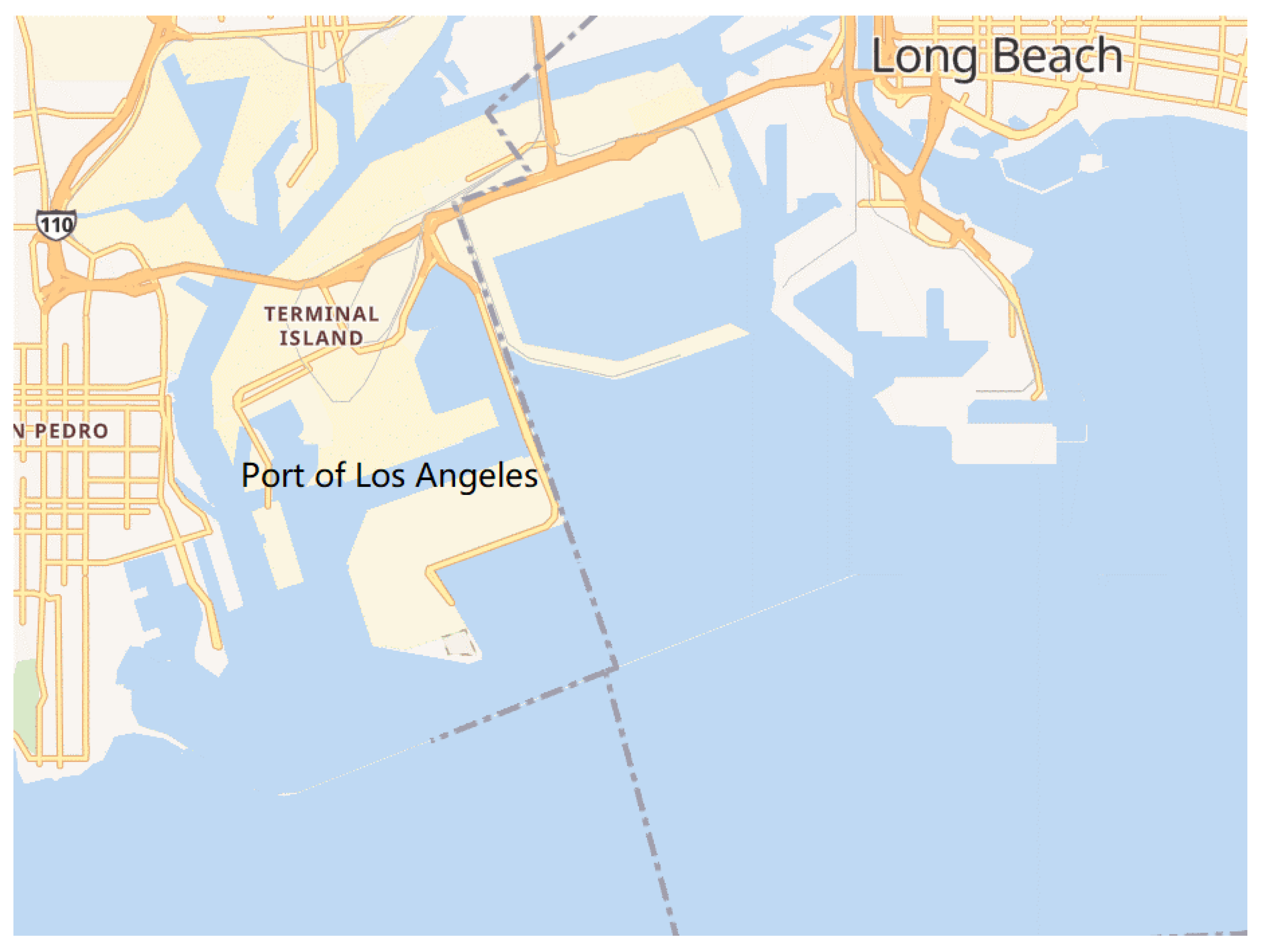
The objectives of this paper are summarized as follows. First, the ports of Los Angeles and Long Beach are taken as the object, and dynamic method, combined with STEAM2, is used to evaluate the ship pollutant emissions, according to the AIS data and ship-related data obtained from the water area of the two ports in 2020. Second, the influence and reasons of ship types, ports, sailing states, and different Emission Control Area (ECA) policies on the distribution of pollutant emissions are analyzed. Third, the effect of ECA policies on ship pollutant emissions is discussed and recommendations are presented to relevant managers.
3. Literature Review
With the continuous strengthening of environmental protection and the development of scientific and technological means, the investigations on ship pollutant emissions have continued to deepen and provide a theoretical basis for the future green development of the shipping market. Jalkanen et al. [
8] conducted a long-term study on the ship pollutant emissions in the Baltic Sea, based on the information provided by the AIS, and established the Baltic Sea ship traffic exhaust emissions inventory from 2006 to 2009. Tokuslu [
9] calculated gas emissions from ships during cruising, maneuvering, and hoteling, in the Port of Samsun, based on ship activity-based methods. Lee et al. [
10] adopted a bottom-up approach to generate the 2019 local ship emissions inventory of the Port of Incheon, and the proposed green emissions policies were applicable in practice.
Shipping is the main source of particulate matter emissions caused by human activities in most parts of the world. Kuittinen et al. [
11] determined the particulate matter emission coefficients of different fuels by measuring the exhaust gas emitted by ship engines, and they used the ship emissions model STEAM to estimate the global shipping particulate matter emissions. Lehtoranta et al. [
12] also investigated the types of fuels used and the impact of marine scrubbers on particulate matter emissions, and they found that the reduction in sulfur content in marine fuels can effectively decrease particulate matter emissions. However, as acknowledged in the discussion, this comparison is invalid because burning natural gas (NG) makes almost all emitted particles smaller than 23 nm. Corbin et al. [
13] indicated that the source of black carbon (BC) and sub-10-nm particles were diesel pilot fuel and lubrication-oil metals. Alanen et al. [
14] suggested that particle number (PN) emissions from marine engines may remain high regardless of sulfur content, mainly due to nanoparticle emissions.
In addition to technological changes and the control effect of international policies on ship pollutant emissions, other external factors will also have an impact on ship pollutant emissions to a certain extent. Xu et al. [
15] evaluated the impact of the epidemic, government prevention, and control policies, as well as the economy on shipping trade in 2020. The growth of the shipping trade will be promoted, to a certain extent, with the control of the epidemic. Luigia and Franco [
16] estimated the generated and saved NO
X, SO
2, and CO
2 emissions by taking the cruise ship during the epidemic, as an example, and analyzed the cruise ship flow during the blockade and in the following months.
Many researchers investigated ship pollutant emissions in China. Numerous studies rely on ports due to a large number of broad-scale ports in China, relatively mature development, and the high availability of various data. According to the trade data of the Port of Qingdao, Liu et al. [
17] established the ship emissions inventory of the Port of Qingdao, from 2005 to 2017, using the trade method and the grey prediction model GM (1,1). An upward trend of CO, NO
X, PM
10, and SO
2 was observed, and the results showed that the four types of pollutant emissions would show a doubling increase in 2030. Yang et al. [
18] established a basic information database of ship emissions in the Port of Tianjin, and they adopted a bottom-up method, on the basis of AIS data, to develop a high-temporal and spatial emissions inventory of ships. Chen et al. [
19] proposed a method for estimating ship emissions inventory based on operating modes, classifying the operating modes of ships with AIS data, and considering three operating modes (berthing, unberthing, and maneuvering) for tugboats. Taking the Port of Dalian as a case study, the model uses different methods to estimate emissions.
China established three ECAs in 2016. Feng et al. [
20] conducted a study on the characteristics of ship pollutant emissions in the Jiangsu section of the Yangtze River waters by using AIS data of the ECA in the Yangtze River Delta waters, using the STEAM2 model to establish a ship pollutant emissions inventory of four major river-crossing bridges in 2017, and analyzing the distribution characteristics of ship emissions. Li et al. [
21] developed a high-resolution ship emissions inventory for the Pearl River Delta region of China, using refined data from the AIS. Ocean-going ships are the largest contributors to total emissions. The spatial distribution of emissions shows that the key emissions hotspots are all concentrated in the newly built ECA.
The nationwide research on pollutant emissions can be mainly divided into two aspects: the pollutant emissions list of inland ships and the pollutant emissions of coastal and ocean-going ships [
22]. Zhang et al. [
23] took Nanjing Longtan Container Port as an example and established a bottom-up activity-based ship emissions inventory by combining AIS data, ship databases, and on-site survey results. Xu et al. [
24] discussed the decision-making behavior of upstream and downstream governments, as well as shipping companies in inland waterway shipping pollution control, based on evolutionary game and prospect theories. Their results showed that the optimal strategy set is active supervision, active supervision, and use of clean energy.
Some studies began exploring the reduction in ship pollutant emissions. Ma et al. [
25] proposed an improved cell-based method, considering ECA regulations and weather conditions. Their findings suggest that this method is effective in reducing costs and ship emissions within the control area, but it may increase the overall emissions for the entire shipping event. Liu et al. [
26] suggested that increasing the level of autonomous ships in the fleet will reduce ship pollutant emissions, and adopting autonomous shipping on major routes can achieve environmental benefits. Ma et al. [
27] also established a multi-objective optimization model for ship route and speed that can simultaneously reduce ship emissions and total costs, considering ECA regulations. Ma et al. [
28] developed a nonlinear mixed integer programming model to address the challenge of simultaneously optimizing the three variables of speed, routing, and refueling strategy to address the constraints for ships, regarding the use of low-sulfur fuel, due to the establishment of ECA. The management of ports and the development of maritime traffic have also attracted the attention of researchers, in recent years, to stay updated with real-time traffic conditions at sea, predict traffic flow to estimate energy consumption, and promote the development of the era of intelligent navigation, which can provide effective information for port ship management and help realize rational management decisions [
29,
30,
31].
According to the existing research, the compilation of international ship emission inventories consists of top-down and bottom-up methods. The top-down methods include the fuel oil method and the trade method, while the bottom-up methods include the statistical method and the dynamic method [
32]. The fuel oil method is suitable for global inventory calculation but not for regional inventory. The trade method has lower requirements for basic data, but it has considerable uncertainty. The statistical method mainly relies on the static data obtained at the early stage, and the dynamic data adopts the estimated value, which has a large uncertainty in the calculation and is suitable for the scope of ports. The dynamic method has the highest accuracy, but it also has higher requirements for basic data.
The largest feature of the dynamic method lies in its mastery of real-time information of the ship’s navigation, as well as its high standards and requirements for the acquisition of the ship’s dynamic information. The dynamic method compensates for the shortcomings of the statistical method to a certain extent. The most significant point is the determination and use of the emission factors of various pollutants. Compared with the statistical method, it reduces the error induced using a unified ship emission factor, to a certain extent, to ignore changes in dynamic factors such as ship sailing states.
The required systems of the dynamic method for the acquisition of ship dynamic data mainly depend on the following: Automated Mutual-Assistance Vessel Rescue System (AMVER), International Comprehensive Ocean Atmosphere Data Set (ICOADS), Long Range Identification and Tracking (LRIT), and the AIS. The establishment time of the first three is earlier than the AIS, and the coverage of Atlantic ships is high, but the penetration rate of ships in Asia is low. The AIS, which was introduced in the 1990s, markedly improved the coverage of ships and enhanced the quality of the acquired data. AIS is a new type of digital navigation aid system equipment, integrating communication and electronic information display technologies. Therefore, the dynamic method in the bottom-up calculation method of ship pollutant emissions will be used in this paper, in combination with the ship traffic emissions model STEAM2, to evaluate the ship pollutant emissions through AIS data and ship-related data.
Our academic contributions are summarized as follows. First, the study analyzes the differences in the distribution trends of ship pollutants in ship types, ports, and sailing states, and it presents corresponding suggestions for relevant managers. Second, this study discusses the impact of California ECA policies on the ports of Los Angeles and Long Beach. Third, the study provides the data basis for relevant departments and international organizations to evaluate the effect of the current ECA policies on the suppression of ship pollutant emissions.
5. Results
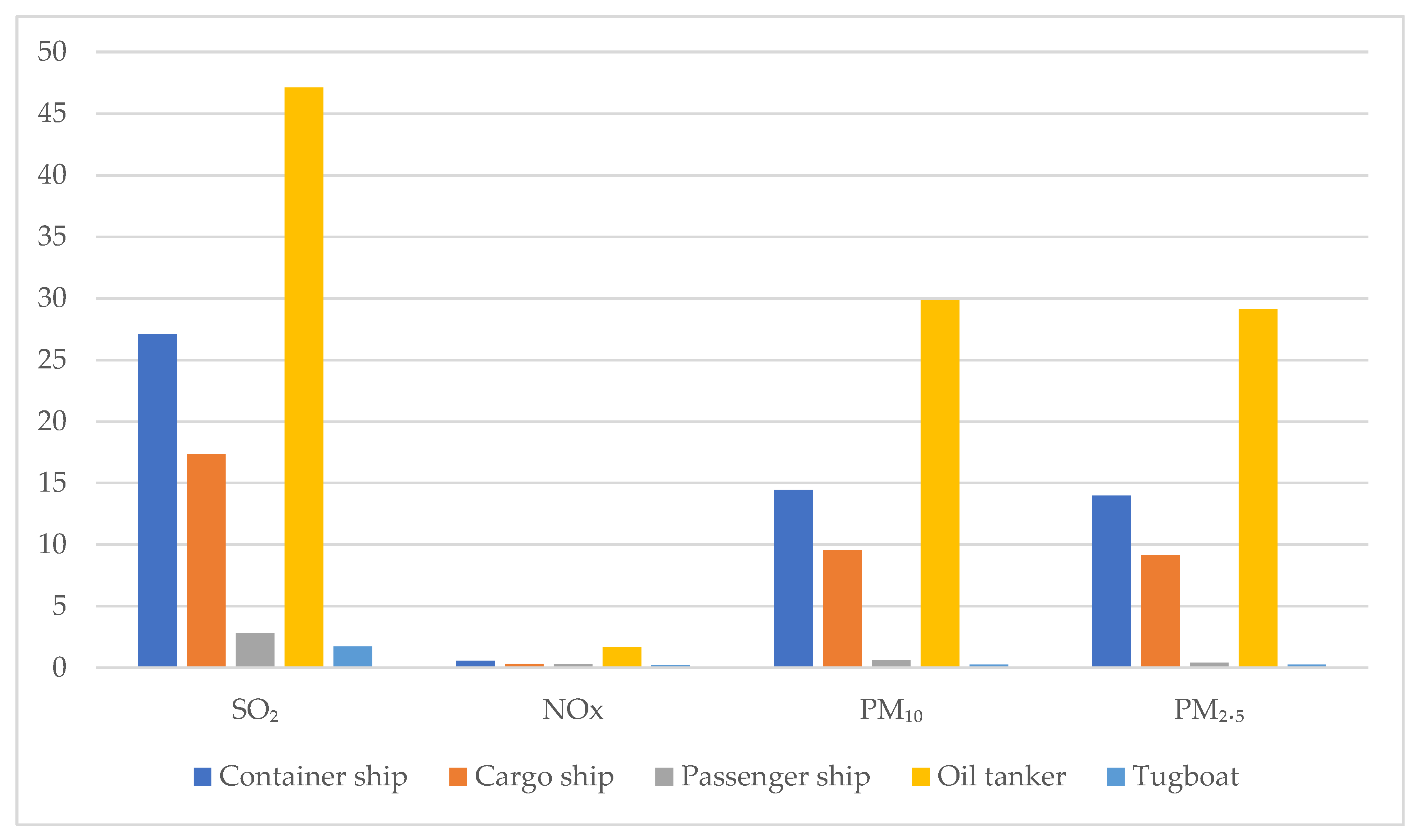
5.1. Comparison of Pollutant Emissions from Different Ship Types
According to the AIS records of ships in the waters of the ports of Los Angeles and Long Beach in 2020, the total emissions of ships calculated for CO, C
XH
X, NO
X, SO
2, PM
10, and PM
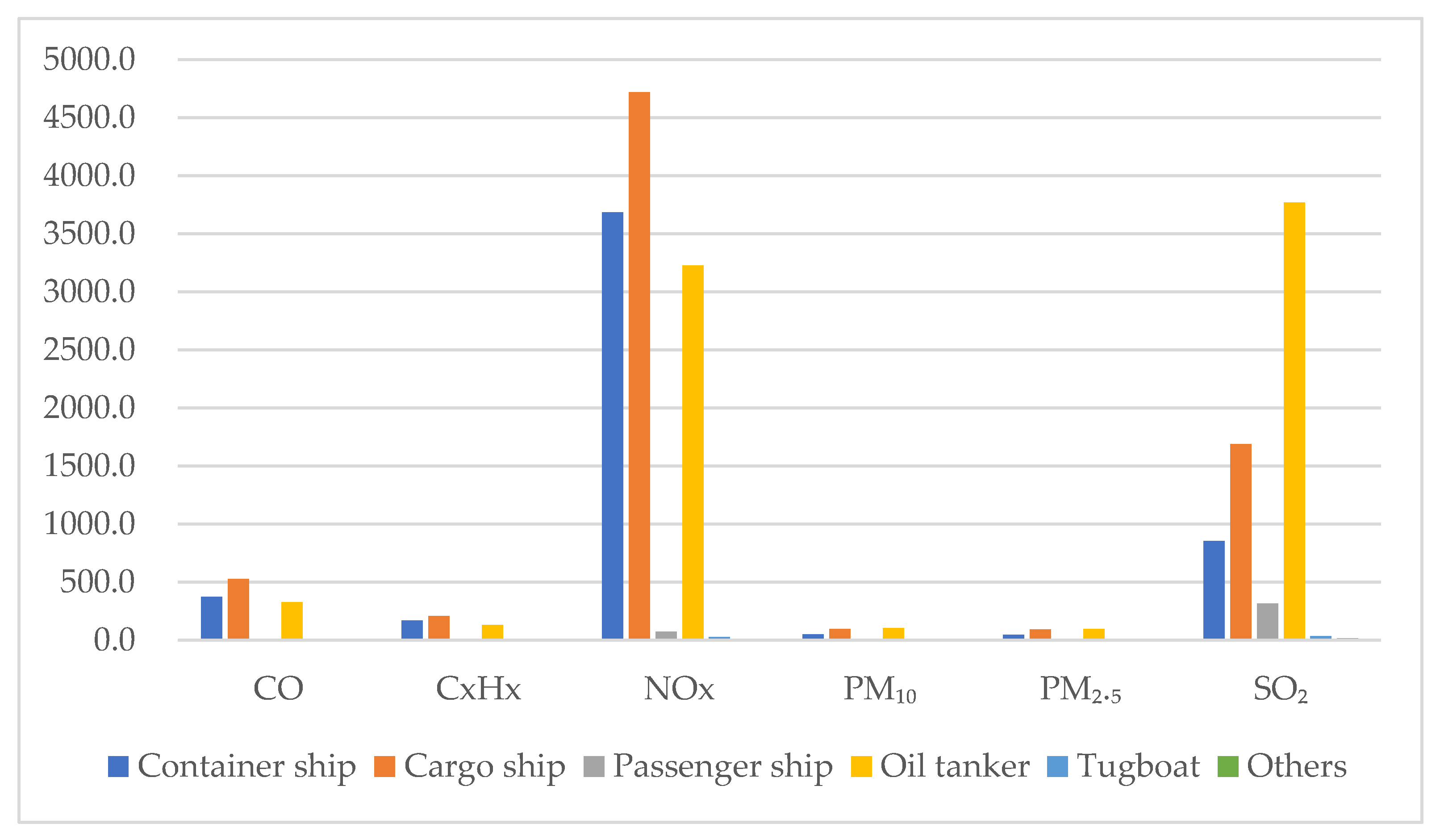
2.5 were 1230, 510, 1170, 6670, 248, and 232 tons, respectively. The comparison of different ship types and their emissions is shown in
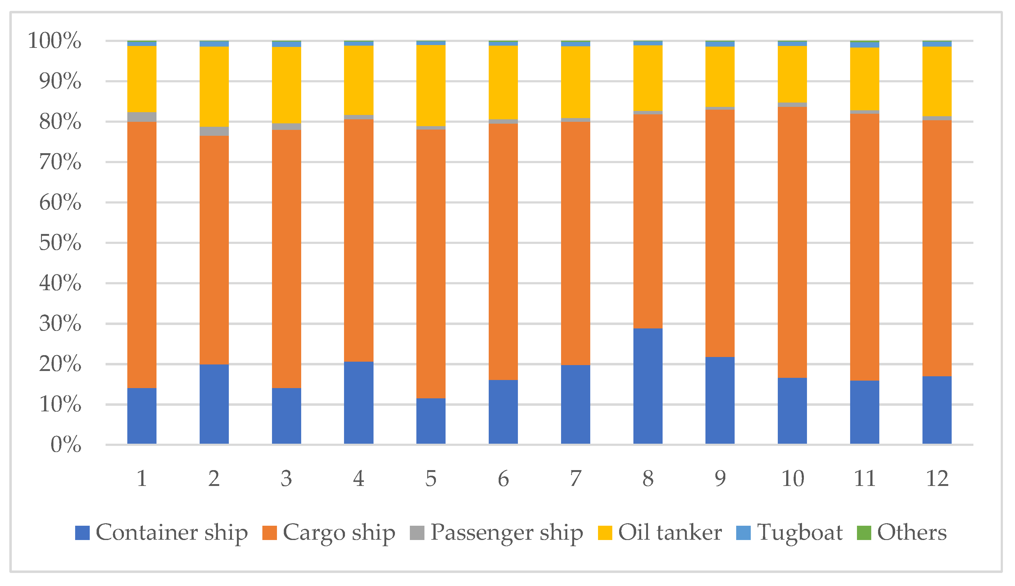
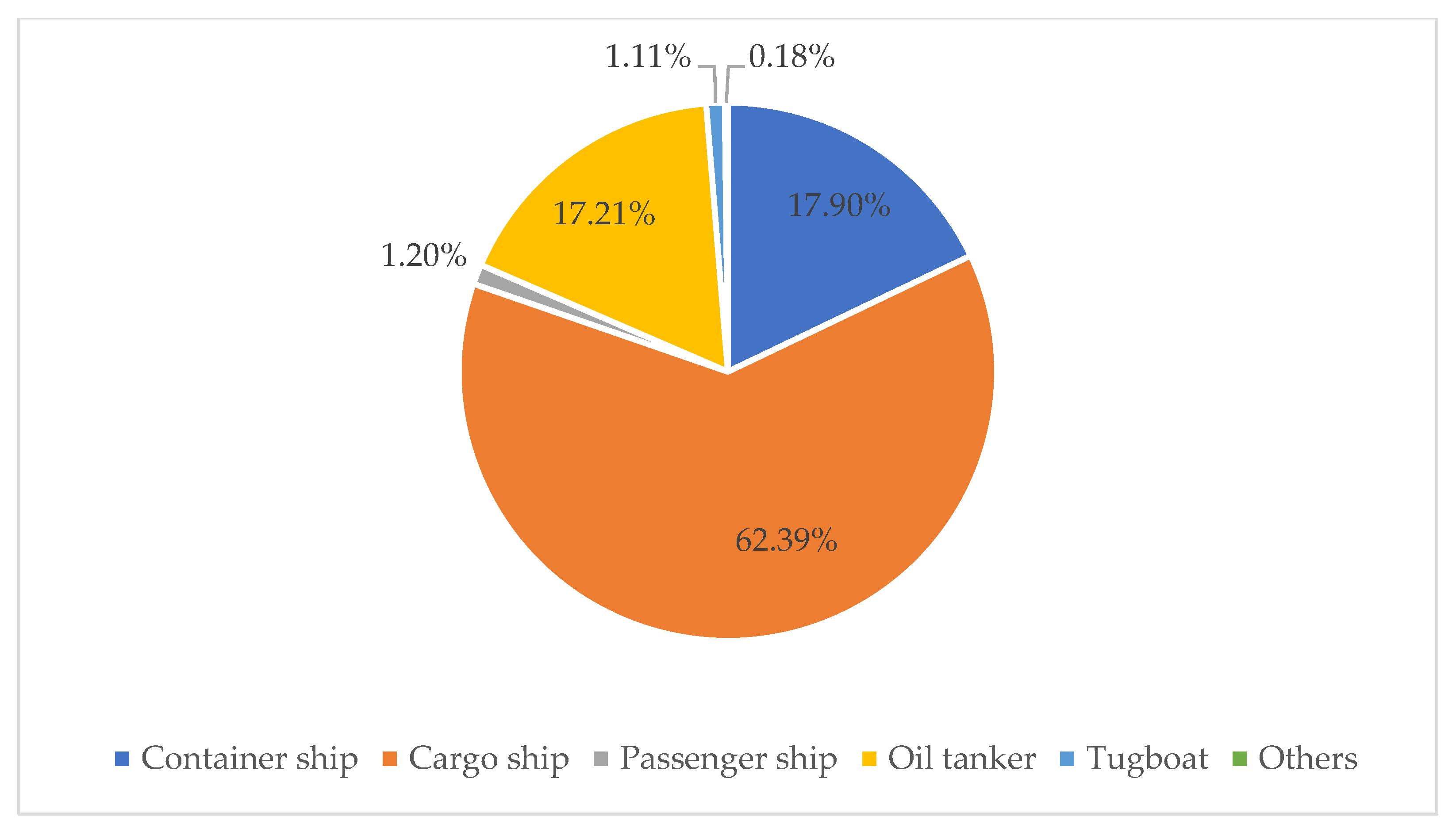
Figure 5. Container ships, cargo ships, and oil tankers are the three most important sources among various types of pollutant emissions. This finding may be attributed to the large proportion of container ships, cargo ships, and oil tankers. The detailed proportions are shown in
Figure 6.
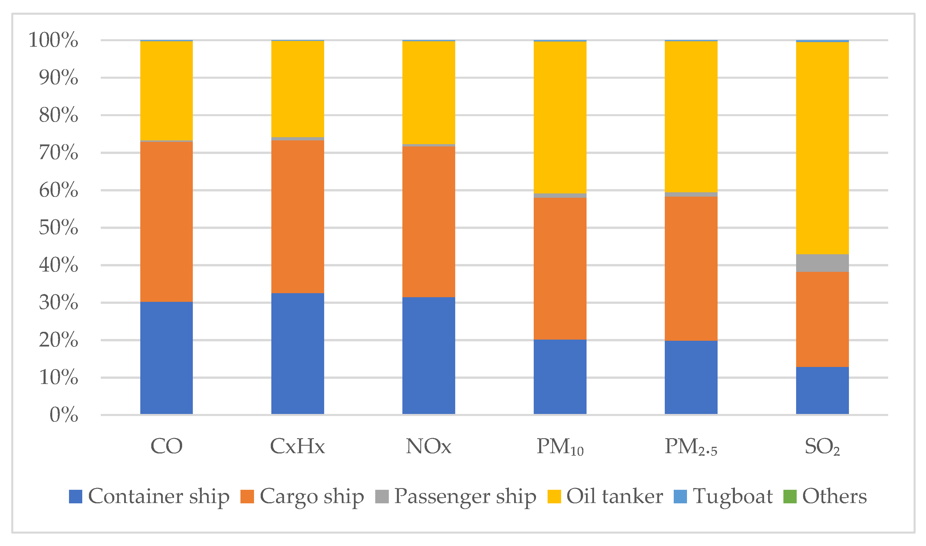
Figure 7 shows the results of re-statistically grouping the overall emissions of ship pollutants, in the waters of the two ports, by ship type. The result indicates that the effects of various ship types on the emissions of CO, C
XH
X, and NO
X demonstrate the same trend: cargo ships are the largest source of the three pollutants, accounting for 40%, followed by container ships and oil tankers, accounting for more than 30% and 25%, respectively; meanwhile, passenger ships, tugboats, and other ship types accounted for the ratio of less than 1%. The reorganization results of the three pollutants, according to the ship type, have the same trend as those in
Figure 6.
The pollutant emissions of cargo ships, container ships and oil tankers are summarized as follows.
(1) The CO emissions from cargo ships, container ships, and oil tankers are 525.3, 372.4, and 326.7 tons, accounting for 42.60%, 30.20%, and 26.50%, respectively.
(2) The CXHX emissions from cargo ships, container ships, and oil tankers are 207.6, 165.8, and 130.6 tons, accounting for 40.70%, 32.50%, and 25.60%, respectively.
(3) The NOX emissions from cargo ships, container ships, and oil tankers are 4717.1, 3684.5, and 3226.9 tons, accounting for 40.20%, 31.40%, and 27.50%, respectively.
This result may be due to the large gap in the size of the ships. Containers are generally manufactured under the implementation of international, national, regional, and company standards [
42]. The size of container ships can be determined in accordance with the maximum carrying capacity. Container ships have different sizes and the largest circulation, but the most frequently used container ships in the world are of a fixed size. Oil tankers also have different classification standards and size specifications. The size of oil tankers has certain standards, which are basically related to the load of the ship itself. Oil tankers have become the largest source of PM
10, PM
2.5, and SO
2 emissions, which are 41%, 40%, and 57%, respectively.
As the first developed maritime transport mode of goods among the three, cargo ships have remarkable inconsistency and spanning in the size of ships. The main reason lies in the inconsistent relationship between ship sailing power and load, due to the differences between national standards. Furthermore, the convenience and economy provided by small-scale cargo ships are one of the reasons why cargo ships are close to container ships and oil tankers when considering pollutant emissions [
43].
5.2. Comparison of Pollutant Emissions in Different Ports
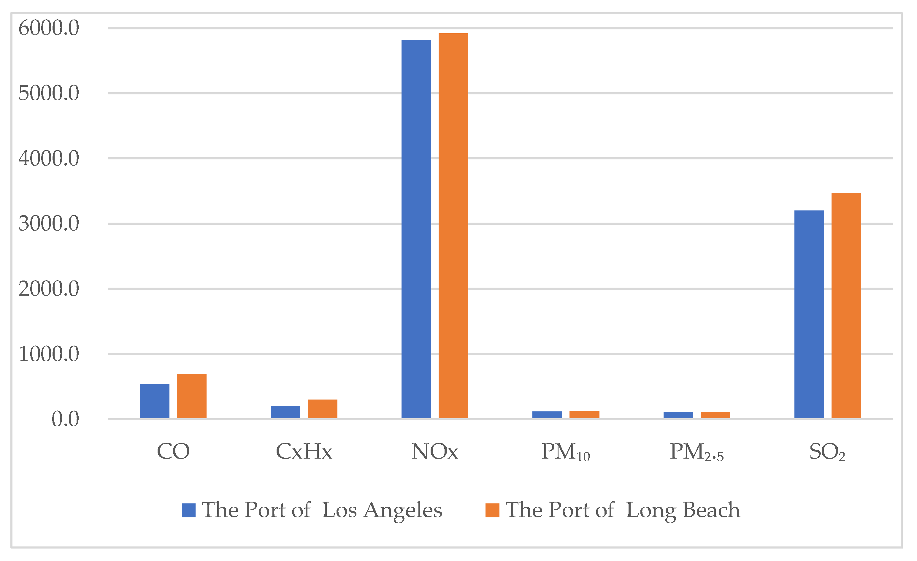
According to longitude and latitude recorded by AIS data, the pollutant emissions may be characterized by spatial distribution, and the comparison of pollutant emissions of the two ports can be obtained, as shown in
Figure 8. The specific situation of the comparison of pollutant emissions between the two ports is shown in
Figure 9. The distribution of pollutant emissions from various ship types in the two ports is highly consistent. The pollutant emissions values of ship types are close to each other. This similarity may be due to the geographical proximity of the two ports, making them all part of the California ECA. Moreover, the closeness allows the two ports to share information resources to a certain extent, apply to the same set of ship emissions regulations, and have the same ship emissions self-control standards and regulatory mechanisms.
Table 10 and
Table 11 show the details of pollutant emissions in the two ports. The pollutant emissions of all ship types in the Port of Long Beach are higher than that of Los Angeles. The reason may lie in the possible effect of the impact of the epidemic in 2020 on global shipping; thus, the production and operation of port ships and other industries will undergo major changes. In the second half of the year, the cargo throughput of the two ports began to rise due to the increase in demand on the Asia–Europe route. However, a serious congestion problem in the Port of Los Angeles simultaneously emerged, and many ships were stranded in the port [
44], thus increasing the incurred expenses of ships at the port and the time cost induced by the inability to deliver on time. Some cargo owners choose air transportation instead to reduce the transportation cost, which decreases the cargo throughput of the port of Log Angeles [
45,
46].
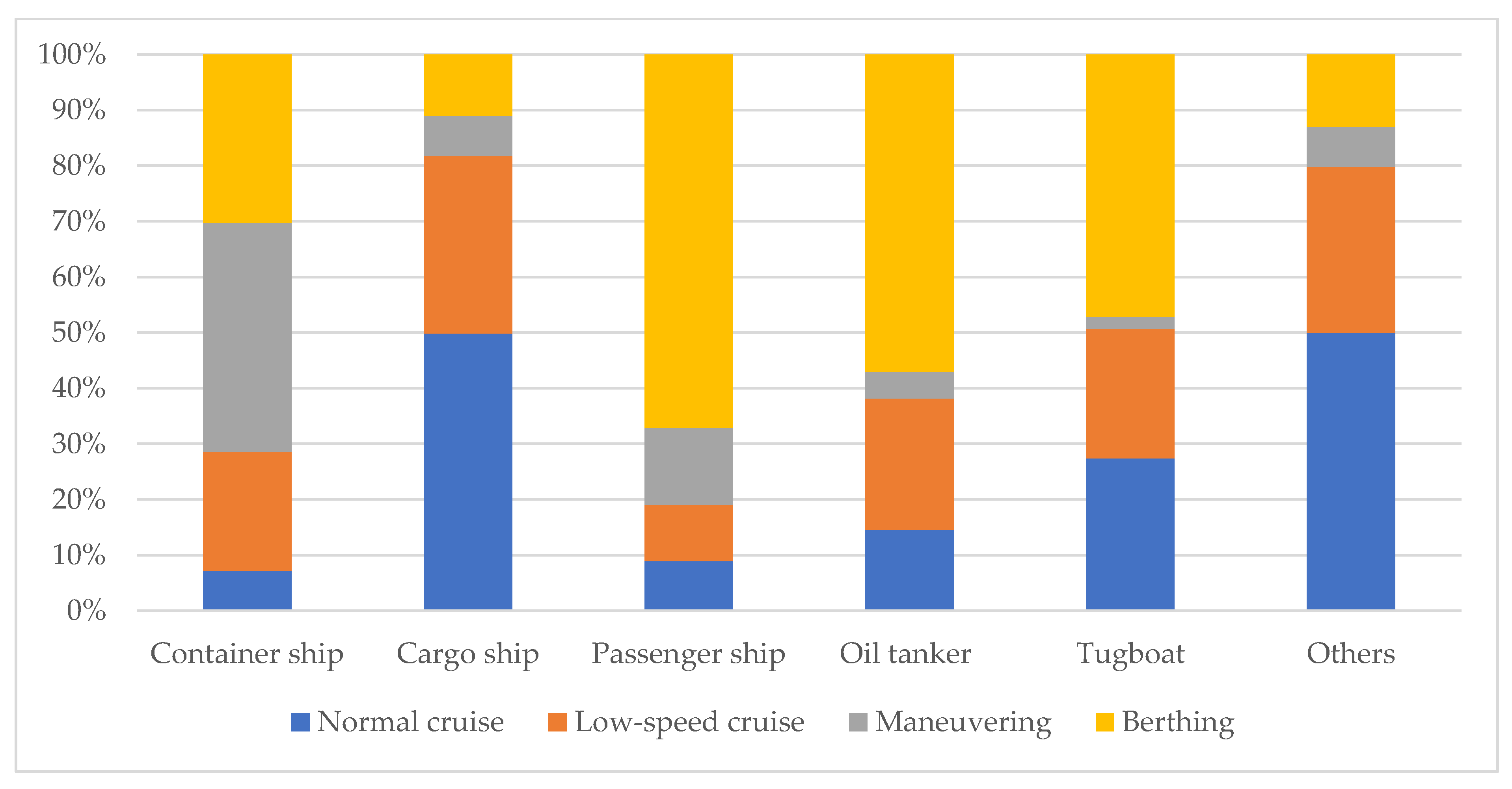
5.3. Comparison of Pollutant Emissions in Different Sailing States
The ratio of pollutant emissions of various ships under different sailing states are obtained as shown in the
Figure 10,
Figure 11,
Figure 12,
Figure 13,
Figure 14 and
Figure 15. The various pollutant emissions from the container ship in the maneuvering state accounts for the largest proportion; CO, C
XH
X, NO
X, PM
10, PM
2.5, and SO
2 provided 42.17%, 41.71%, 40.02%, 45.31%, 44.80%, and 35.05%, respectively. This finding is related to the development trend of containers, as shown in
Figure 16. At the mature stage, from the end of the 1980s to the present, the transportation mode of container ships no longer pursues simple high-speed development due to various factors. On the one hand, container shipping companies have reduced the speed of ships in the process of sailing to minimize oil consumption because of the soaring oil price. On the other hand, in coastal areas, especially in areas with intensive human activities, the speed of container ships will be reduced to less than 10 nautical miles per hour to pursue green development [
47]. These reasons contribute to the speed reduction in container ships in port waters, resulting in the largest proportion of pollutant emissions in the maneuvering state.
The pollutant emissions of cargo ships in normal cruising are remarkably higher than in other states. The proportions of each pollutant emissions for CO, CXHX, NOX, PM10, PM2.5, and SO2 are 47.03%, 49.84%, 48.05%, 51.10%, 50.97%, and 42.37%, respectively. This finding may be attributed to the limited import and export of goods in the United States in the first half of 2020, due to the dual impact of the epidemic and the China–US trade war.
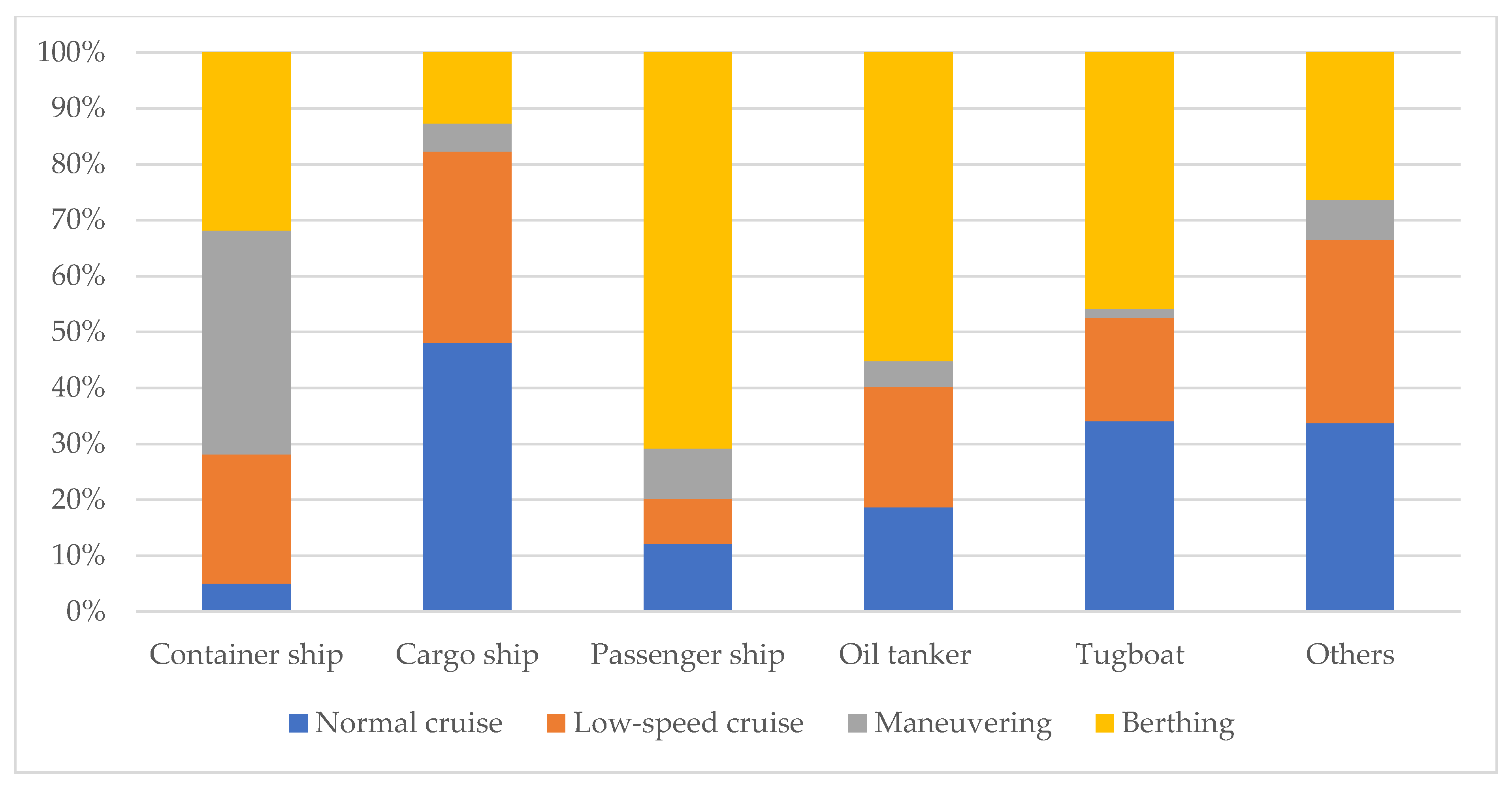
Simultaneously, the proportion of pollutant emissions of passenger ships in the berthing state is the largest. The proportions of each pollutant emissions for CO, C
XH
X, NO
X, PM
10, PM
2.5, and SO
2 are 63.08%, 67.12%, 70.80%, 82.16%, 81.37%, and 85.21%, respectively. The key measure to cause this phenomenon lies in termination of the related operations of passenger ships in the two ports in mid-March 2020 and the spending of additional time of most passenger ships at berths [
45,
46].
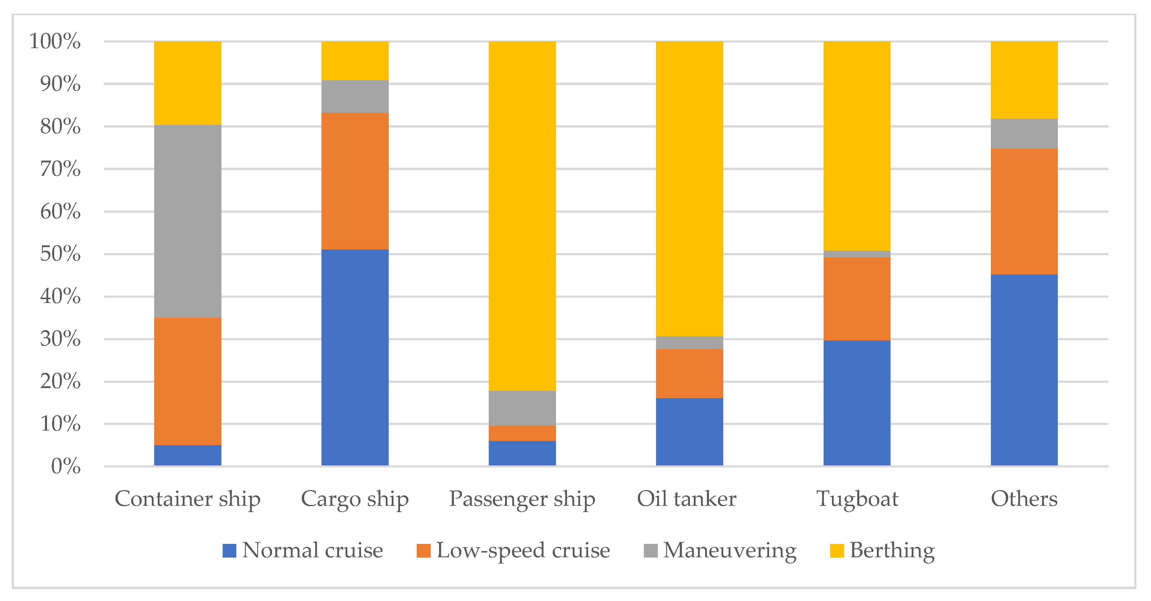
The proportion of pollutant emissions of oil tankers in the berthing state is the largest. The proportions of each pollutant emissions for CO, CXHX, NOX, PM10, PM2.5, and SO2 are 56.73%, 57.12%, 55.20%, 69.32%, 68.55%, and 86.14%, respectively. The operating staff at the ports became insufficient in 2020 due to various reasons (such as the epidemic), resulting in a decrease in the efficiency of cargo loading and unloading.
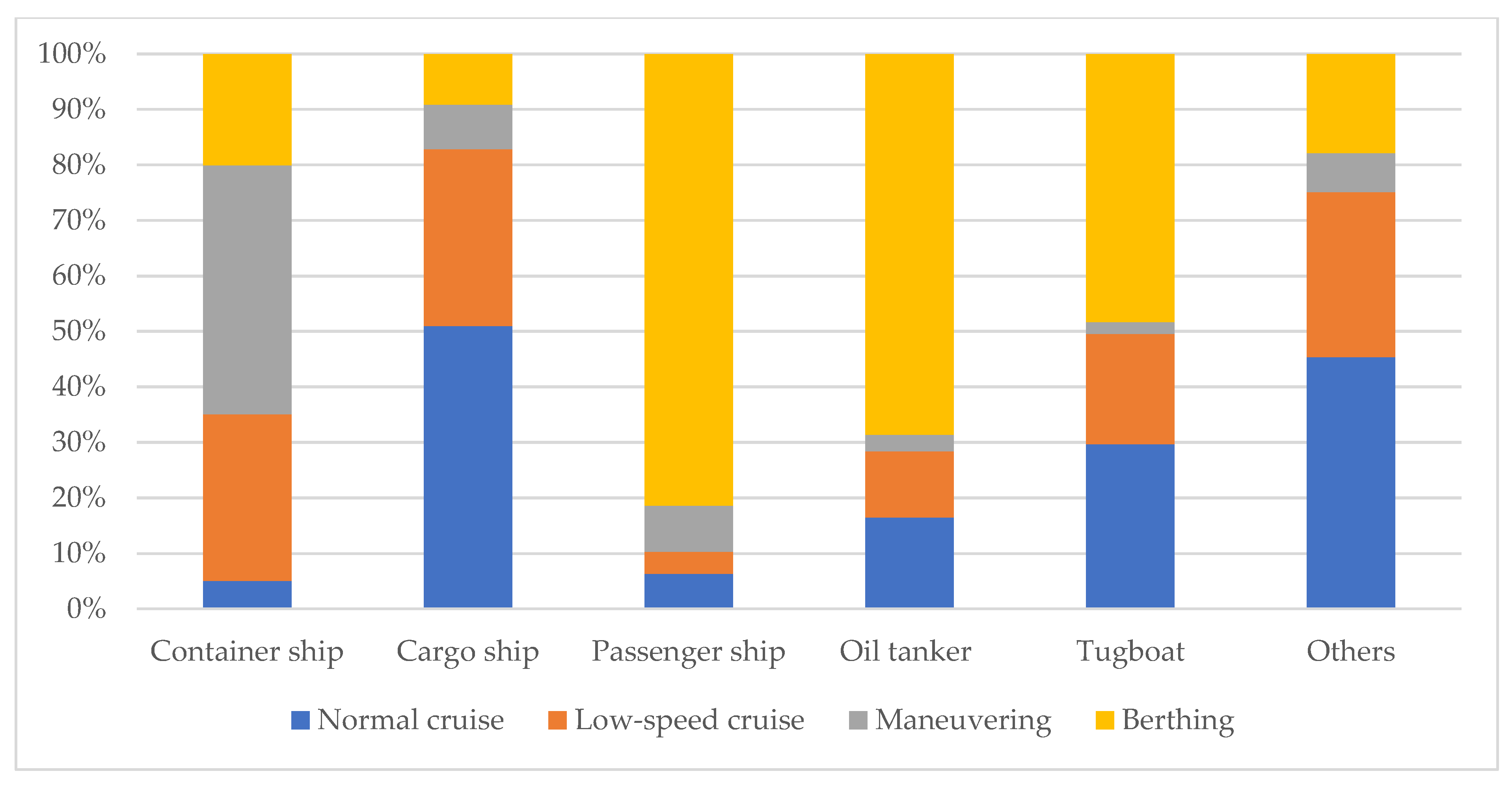
Tugboats are port operation ships that assist other ship types to complete port berthing and departure activities. Thus, their pollutant emissions status is generally related to the activities of other ships and changes with the demand of the external environment. Among them, the proportion of each pollutant emissions in the berthing state is the highest. However, emission factors cannot be determined for other ships. Thus, the cargo ship emission factor is used for calculation in this study to avoid introducing excessive bias to the results due to the omission. Therefore, cargo ships have similar results.
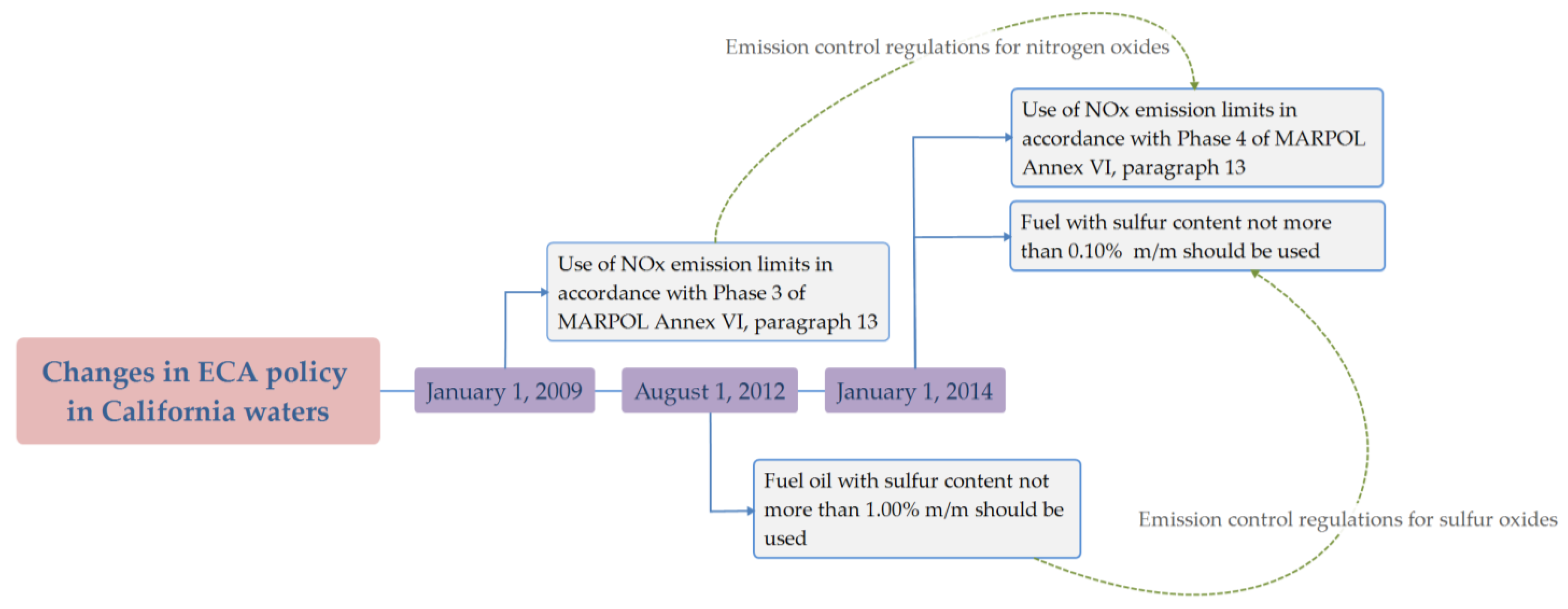
5.4. Comparison of Pollutant Emissions under Different Policies
The emission factors of the Phase II and Phase III are shown in
Table 12 [
22,
40], and the emission factors of SO
2, PM
10, and PM
2.5 are calculated. The formula is the same as before, except that the sulfur content in the fuel used in the formula will be changed from 0.1% to 1% [
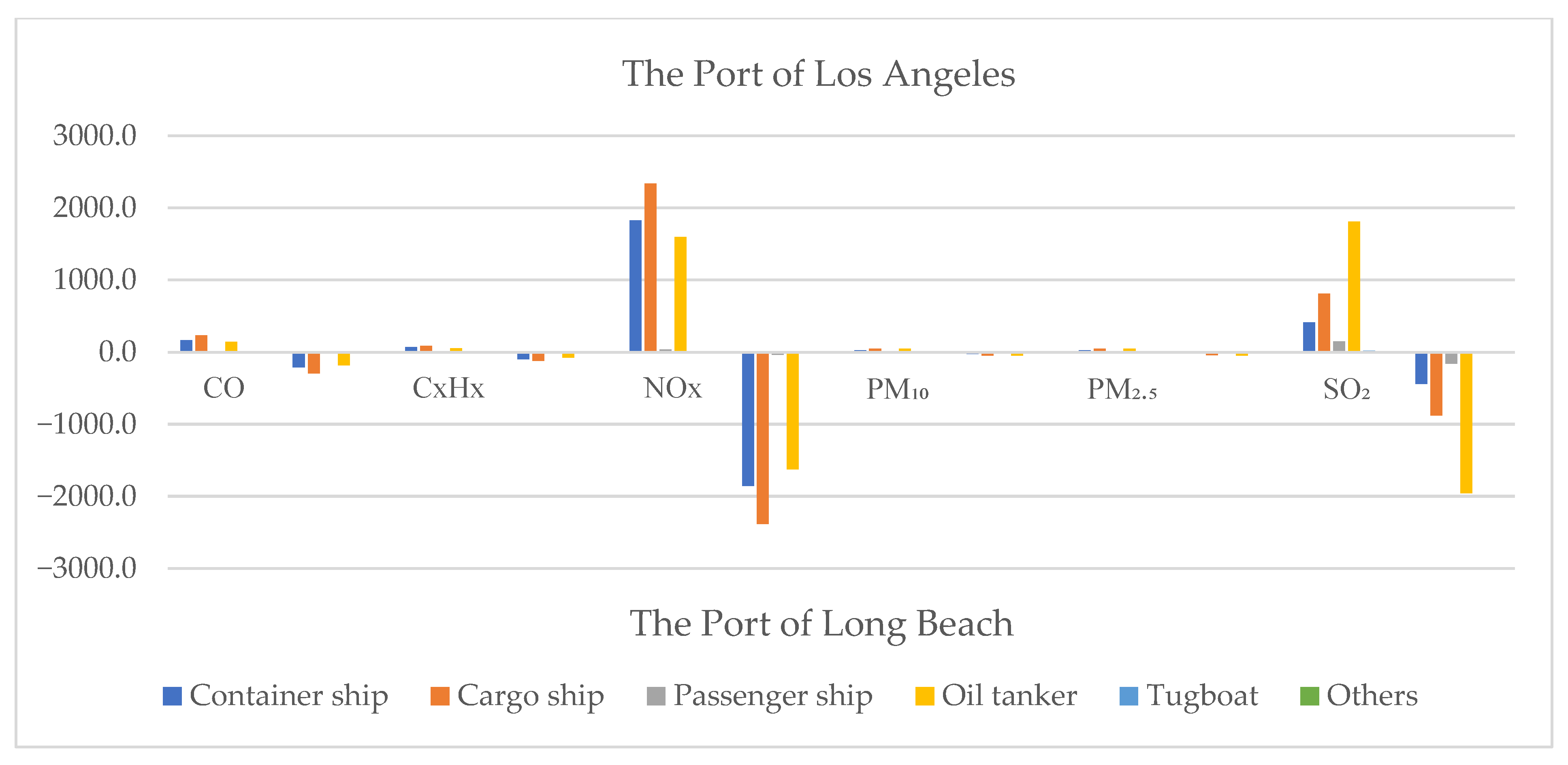
5]. According to the different requirements of each pollutant emissions limit, at different stages of the California ECA, and the adjustment results of the relevant pollutant emission factors, the changes in ship pollutant emissions are shown in
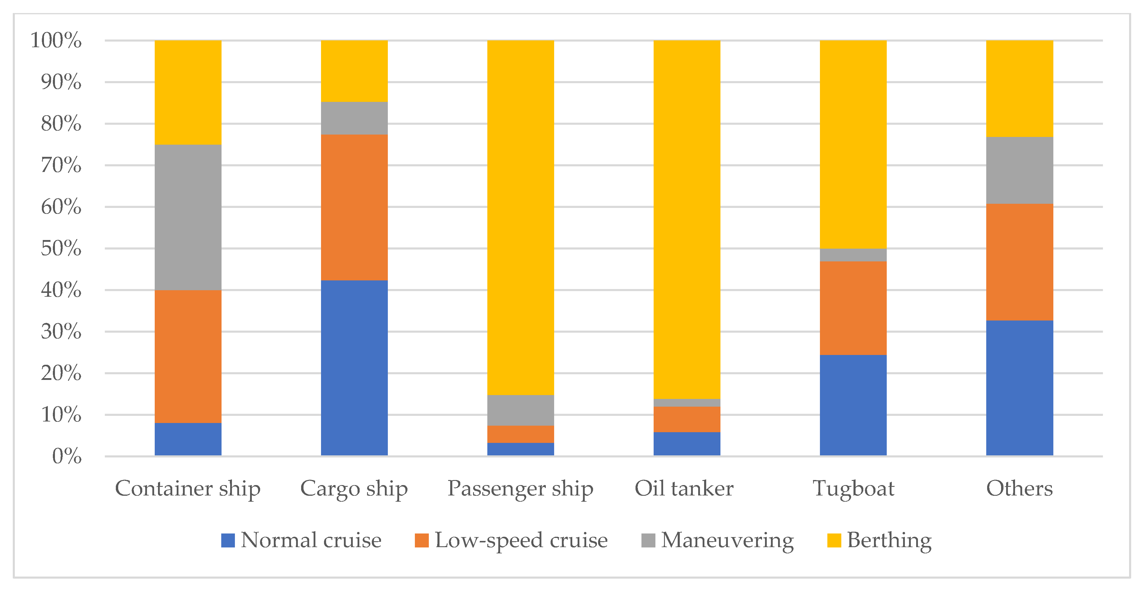
Figure 17.
Comparing the changes in the emissions of the four major pollutants caused by the two-stage policies, the change in SO
2 is the most evident. Compared with Phase III, the specific changes in SO
2 emissions of various ship types in Phase II are as follows: container and cargo ships, respectively, increased by 27.12% and 17.36%; passenger ships increased less with 2.78%; oil tankers increased the most with 47.13%; the upward trend of tugboats is the smallest, demonstrating only 1.73%. These changes are caused by the variations in the sulfur content of marine fuels, due to the two-stage ECA policies [
5], thus leading to a different subsequent determination of the SO
2 emission factor. The ECA policies are effective in suppressing SO
2 emissions. However, the NO
X emissions of various ship types did not demonstrate substantial change. Only the emissions of oil tankers in Phase II increased by 1.71% compared with Phase III. The NO
X emissions of other ship types changed slightly and did not increase by more than 1%. The changes in the emissions of PM
10 and PM
2.5 are relatively evident.
The ECA policies can effectively reduce the emissions of ship pollutants, especially for SO
2, but the effect on NO
X is not observed. The comparison of pollutant emissions in the state of ship sailing reveals that passenger ships, oil tankers, and tugboats have the highest proportion of pollutants in the berthing state. During the epidemic period, ships stay at ports for a long time due to the requirements of epidemic prevention and control policies, resulting in increased pollutant emissions. Ships must use expensive low-sulfur fuel within the ECA range. However, ships usually choose to use high-sulfur fuel oil outside the ECA and switch to low-sulfur fuel when approaching the ECA. Ships choose to sail for a long time outside the ECA to control costs [
48]. Chang et al. [
49] analyzed the impact of the implementation of ECA policies on the efficiency of European ports, and they indicated that the implementation of ECA policies reduced productivity of ports due to strict regulation. In addition, NO
X accounts for a high proportion of the overall pollution. However, the ECA policies have not played a satisfactory role in suppressing NO
X emissions. Thus, measures to reduce NOx emissions should also be considered.
6. Discussions
This paper has some limitations. The impact of ship power systems on ship pollutant emissions is not reflected. Some errors in AIS data may also be observed. AIS equipment is divided into classes A and B when determining the sailing time. Many class B ships are observed, affecting the reception of class A ships [
50]. AIS data is generally poor in places where the number of ships is dense, which will have a certain impact on data collection and accuracy.
The results of our study are compared with other studies on the specific impact of ECA policy implementation on pollutant emissions in China. Shi et al. [
40] compared the changes in pollutant emissions from ships of various types, after the implementation of the ECA policies at different stages, in the waters of Shanghai Port using the AIS data in 2017. At stage V, all ships in the Shanghai Port were required to use fuel with a sulfur content of 0.1%. Compared with the benchmark policies, NO
X, SO
2, and PM
2.5 emissions from cargo ships decreased by 4.3%, 91.48%, and 73.93%, respectively. Zhang et al. [
51] focused on the performance of the ECA policies in Shanghai, considering SO
2 concentration. The SO
2 concentration in Shanghai decreased by at least 0.229 μg/m
3 daily on average. Similar to the current findings, ECA policy can effectively inhibit SO
2 emission, and the inhibition effect on SO
2 is significantly larger than that of NO
X. NO
X and SO
2 are the largest pollutants in our research. The research of Yang et al. [
18] used the bottom-up research method, considering the proportion of various pollutants to the total, to establish a pollutant discharge inventory of Tianjin Port based on AIS data. The total ship pollutant emissions for CO, NO
X, SO
2, PM
10, and PM
2.5 were 2210, 28,610, 14,530, 2040, and 1820 tons, respectively. As with the obtained findings of the current study, NO
X is the main pollutant, accounting for 56.9%, followed by SO
2, which accounts for 28.9%. They also considered the impact of the engines, wherein the main engines were the largest sources. The impact of the engine on pollutant emissions was disregarded in the current study. Lee et al. [
52] used a bottom-up activity-based approach, combined with real-time vessel activity data generated by Vessel Traffic Services (VTS), and found that NO
X and SO
2 accounted for the largest proportions of overall emissions.
The distribution of pollutant emissions from ships is affected by the development of the epidemic, the ECA policies, and the speed of ships. The speed is influenced by the weather and it affects the emissions of pollutants. In 2020, the AIS records of the two ports accounted for the highest proportion of cargo ships, with 62.39%.
Figure 2 shows that the concentrated distribution is relatively dense in May, June, and July, and the ship traffic volume is high in summer [
53]. Encountering wind and waves will have a certain impact on the speed of the ship, thereby affecting its activities and pollutant emissions. However, this effect is not evident in the port area.
SO
2 and NO
X account for a relatively high proportion of the total ship pollution emissions. SO
2 and NO
X account for 32.0% and 58.2% in the Port of Los Angeles, while SO
2 and NO
X contribute 32.6% and 55.7% in the Port of Long Beach. The pollution to the atmospheric environment mainly comes from the use of engine fuel. Before the ship emissions control, the high sulfur content in the heavy oil used by ships is one of the main driving forces to increase the SO
2 content in the atmospheric environment. Sulfur oxides produced by shipping form strong acids and seriously affect biodiversity [
54]. Most ships will be equipped with high-power engines and use fossil fuels, accelerating energy consumption. Ships also pollute the water environment. On the one hand, the wastewater is poured into the waters where the ship sails. On the other hand, the domestic sewage and garbage generated by the crew in their daily lives contribute to pollution [
55]. These reasons deplete the availability of seawater as a resource and destroy the living environment of marine organisms, which is not conducive to ecological balance. The NO
X generated by ship transportation produces eutrophic water [
56]. Additionally, the decline in water quality affects the survival of marine plankton, resulting in the loss of biodiversity, which leads to changes in the food web in the waters and hinders the development of local fisheries [
57].
These pollutions to the environment will eventually affect people’s daily life and health. The discharged sulfur from ships is a factor that can form acid rain, destroy the soil, and increase acidity [
58], which seriously affects the development of agriculture, forestry, and fishery in related areas. Relevant studies have shown that the particulate matter emitted by shipping activities causes approximately 60,000 deaths yearly due to cardiopulmonary diseases and lung cancer [
59]. The use of low-sulfur oil can reduce deaths by 34% and morbidity by 54% due to ship pollutant emissions. Low-sulfur oil has markedly reduced the side effects of shipping activities on human health; however, pollutants, such as emitted particulate matter, are still responsible for 250,000 deaths and approximately 6.4 million childhood asthma cases yearly [
60].
Our study evaluated ship pollutant emissions in the ports of Los Angeles and Long Beach, the two busiest ports in the United States, so the impact of ECA policies on ship emissions from these two ports is relatively representative. The California state gradually has a multi-level legislative system, ranging from international conventions to the federal and state levels, in terms of ports and implements strict emission control regulations to promote the green development of the port. In 2006, the two ports jointly implemented the San Pedro Bay Port Clean Air Action Plan, including fuel switching and ship speed reduction [
35].
Our results show that NOX accounts for a large proportion of ship pollution emissions, but the ECA policy has not played a good role in suppressing NOX emissions. It is necessary for relevant organizations, in various countries, to focus on how to effectively suppress NOX emissions through policy control worldwide in the future. In addition, the sailing states also markedly affect the ship pollutant emissions. The staying time in the ports needs to be minimized. In addition to optimizing the port loading and unloading processes, governments should also take other measures to ease port congestion, such as slowing down the speed to delay the arrival time and avoid many stranded ships at the ports, causing additional pollution to the port waters.
Although the control effect of low-sulfur oil on the emissions of pollutants from ships has been reflected in the research, the high price of low-sulfur fuel makes many ships choose to use high-sulfur fuel outside the ECA area to reduce costs, which may not have a remarkable inhibitory effect on worldwide pollutant emissions [
48]. The implementation of ECA policies around the world should also consider the cost of ship operation, combining environmental and economic sustainability. In this case, other measures may also be used to offset the impact of the sulfur content in the fuel, such as utilizing marine scrubbers. Simultaneously, different emission limits and fuel standards may be formulated in accordance with the severity of ship pollutant emissions from various ships. Marine cleaning equipment should also become one of the important means to reduce pollutant emissions.
7. Conclusions
This paper investigates the ship pollutant emissions in the waters of the ports of Los Angeles and Long Beach in 2020, based on the AIS data and related ship data, and it evaluates the change in the ship pollutant emissions under the two-stage ECA policies. The main results are as follows. (1) The emissions of each pollutant for CO, CXHX, NOX, SO2, PM10, and PM2.5 were 1230, 510, 11,700, 6670, 248, and 232 tons, respectively. (2) In the emissions of various pollutants, container ships, cargo ships, and oil tankers are the three most important sources, and the total emissions of ship pollutants generated by the three account for almost 90% of the total pollutant emissions. (3) The ports of Los Angeles and Long Beach have the same trend in ship pollutant emissions. The specific pollutant emissions in the Port of Long Beach are slightly higher than in the Port of Los Angeles. (4) The distribution of pollutant emissions, of different ship types in each sailing state, is different. Container ships have the highest proportion of pollutant emissions in maneuvering state, while cargo ships in normal cruising state have a higher proportion than other ship types. Passenger ships have the largest proportion in berthing state. The proportion of tugboats in each sailing state does not show a clear bias. (5) Considering the change in the ECA policies in the California ECA, the changes in the emission factor are used to evaluate the detailed variations of the two-stage ECA policies. The results show that the ECA policies have the strongest inhibitory effect on the emissions of SO2, especially for the control of SO2 emissions from oil tankers. Compared with Phase III, the relaxed ECA policies in Phase II increased the SO2 emissions of oil tankers by 47.13%.
Regarding the future research in the ship pollutant emissions calculation, different ship power systems, as well as the differences in ship pollutant emissions of various engine types, can be highlighted to provide new development directions for the construction of ship power systems and the selection of fuels. Simultaneously, the scope of the research is expanded to obtain the realistic results, which can provide real-time data for the monitoring of pollutant emissions in the ports and present effective information for the management and control of ships in the ports.


