Article

A Numerical Performance Analysis of a Rim-Driven Turbine in Real Flow Conditions

1
School of Mechanical and Electrical Engineering, Kunming University, Kunming 650214, China
2
Faculty of Mechanical and Electrical Engineering, Kunming University of Science and Technology, Kunming 650500, China
*
Author to whom correspondence should be addressed.
J. Mar. Sci. Eng. 2022, 10(9), 1185; https://doi.org/10.3390/jmse10091185
Submission received: 29 July 2022 / Revised: 21 August 2022 / Accepted: 21 August 2022 / Published: 25 August 2022
(This article belongs to the Topic Marine Renewable Energy, 2nd Volume)

Abstract

:
The tidal turbines represent a new frontier for extracting energy from tides source. Despite the technology being mature, new solutions aimed at improving performance, reliability with reduced environmental impact, manufacturing and installation costs are currently under investigation. The Rim-driven turbine (abbreviated as RDT) was recently proposed. A RDT resembles a ducted turbine (abbreviated as DT), as both contain blades and a duct. The present study aims at investigating the detail performance and flow field of a RDT in a real flow based on the China Zhaitang Island’s tidal current data. To show the difference between the RDT and DT, simulations are also performed on the corresponding DT. It is found that the power and thrust for the two configurations exhibit time-periodic behavior that is consistent with the wave frequency. At axial flow, the fluctuation amplitude on the power and thrust increase with the increase of tip speed ratio. The RDT has higher power output when operating at lower tip speed ratio and has a potential reduction in flow resistance and disturbance with respect to the DT. At yawed flow, the fluctuation amplitude on the power and thrust decrease with the increase of yaw angle. The RDT has less capable of compensating the effect of yawed inflow in reducing the power than the DT at larger yaw angle. In addition, the power and thrust generates micro-amplitude fluctuation integrated into the main waveform, which the frequency is consistent with the turbine rotation frequency. The wake characteristics analysis reveals that the yawed flow field is more turbulent, and the two configurations suffer strong unsteady flow separation along the whole span. Strong interactions are observed between the rotor’s main wake and the duct’s upper wake. The yaw angle primarily determines the downstream wake deflection direction and significantly changes the wake shape and vortex structures. Meanwhile, the wake flow is found to recover more quickly at larger yaw angle. Besides, due to the open-center of RDT, a part free-stream flow is allowed to travel through and forms an obvious high velocity zone. The presence of open-center of RDT has avoided the low velocity zone, improved the wake structure and accelerated wakes recover, which seems to give an advantageous effect in operating a RDT.

1. Introduction

Energy issue is one of the main factors for economic development. Most countries and regions seem to be dependent on fossil fuel to fulfill their needs. Efforts are being made to duel with environmental pollution and fossil fuel consumption, better in terms of performance and economy, to cope up with the swelling demand of energy. The past few years have seen an increase in worldwide interest of using renewable energy (e.g., wind, solar, tide, wave, geothermal, biomass, etc.) to generate electricity [1]. Each of these energy resources is distributed globally. Tidal current energy, utilizing tides, is predictable many years in advance, which provides a reliable resource with significantly greater in its energy density compared to other renewable energy [2,3]. In addition, tidal current energy allows designers to limit visual exposure, acoustic disturbances and to reduce environmental impacts. Tidal turbines (similar to wind turbines) are devices designed to extract the power from tides source, which represent a new frontier for extracting energy. Tidal turbines can be generally classified into two types according to the operation mode, the horizontal axis turbines and the vertical axis turbines [4,5]. Among the two types, horizontal axis turbines with two or three blades currently dominate the sector [6], accounting for about three quarters of companies developing such devices due to its higher efficiency [7].
In recent years, tidal turbines, via theoretical, numerical and experimental analyses, have been studied and remarkable results and progress have been achieved [8,9]. Despite the technology being mature, new solutions aimed at improving performance, reliability with reduced environmental impact, manufacturing and installation costs are currently under investigation. For example, blades optimization based on genetic algorithm is a way to improve turbine’s performance by increasing blade lift and reducing blade drag [10,11]. The adoption of contra-rotating rotors is also a way to improve turbine’s performance. It allows the achievement of enhanced performance than single rotor turbine, and the advantages in terms of structure and mooring arrangement are achieved owing to the near-zero reaction torque on the supports [12,13,14]. Another way is the adoption of diffuser-augmented turbine or ducted turbine (DT), which leads to an enhanced performance by increasing the flow velocity at the “throat” where the rotor is placed and keeps the size of the moving components to a minimum, thus reducing manufacturing as well as operating and maintenance costs [15,16,17,18]. However, in a DT, the blades and the generator need supports to fix, and the generator and supports occupy a lot of space, and may cause some interference to the internal flow field. In order to overcome this drawback, drawing a lesson from the latest research on marine propulsion of Rim-driven system [19,20,21,22], the Rim-driven turbine (RDT)was recently proposed. In a RDT, with rim-driven topology the electromagnetic system equipment is inserted in a structure with a certain hydrodynamic shape like a hydrodynamic duct. No extra supports and external power generation equipment are required which allows to minimize the volume of the supports and extra structure and to maximize the compactness and the robustness of the system. Figure 1 shows the principle comparison between a ducted turbine and a Rim-driven turbine. It can be observed that the RDT is similar to a DT in its structural design, as both contain blades and a duct. It is worth mentioning that using a ducted configuration not only leads to improve the performance, but minimize cavitation and vibration, and play a role in the blades protection. This is why the RDT can be a very attractive solution to reach the design goals of a tidal turbine dedicated to energy generation. Recently, Borg et al. [23,24] numerically analyzed the hydrodynamic performance and structural response of a RDT. Song et al. [25] numerically analyzed the flow energy loss characteristics of a RDT. Djebarri et al. [26,27] numerically analyzed the electromagnetic characteristics of a flux PM generator on RDT. Feng et al. [28] experimentally and numerically tested the performance of a RDT array. In addition, the OpenHydro turbine is one of few examples of an industrial RDT [29].
Literature research shows that very few academic or industrial demonstrations on the Rim-driven turbine (RDT) have been introduced for the time being. Besides, when in a real marine environment, a RDT will face shear flow, turbulence, directional changes in tides and wave-current interaction. Understanding the performance in such environment is becoming more prominent and necessary for designing work. Moreover, as a RDT resembles a DT, understanding the performance difference between the two configurations is also an important issue. Hence, to address the uncertainty in the performance, the following study focuses on investigating the detailed performance and wake characteristics of a RDT and the corresponding DT in real flow conditions via the computational fluid dynamics (CFD) tool. The results of this work help provide further insight into each performance and to further understand the wake characteristics from a RDT and a DT. The remainder of this article is structured as follows: Section 2 deals with the methodology, model and mesh setup, and numerical validation. Section 3 discusses the results obtained from the parametric analysis. Section 4 deals with the conclusion, which summarizes the key results obtained from this study.

2. Numerical Methods

2.1. General Features
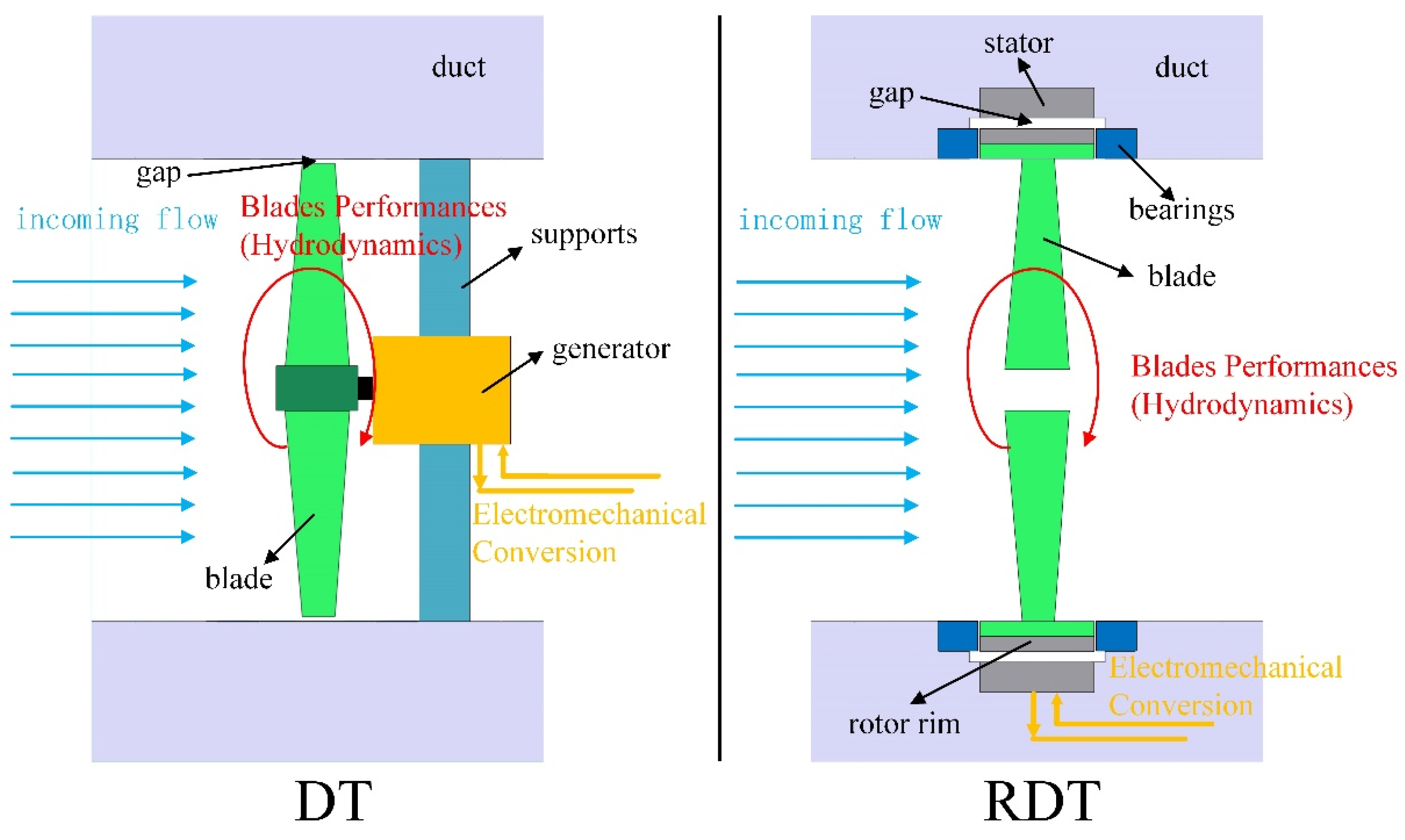
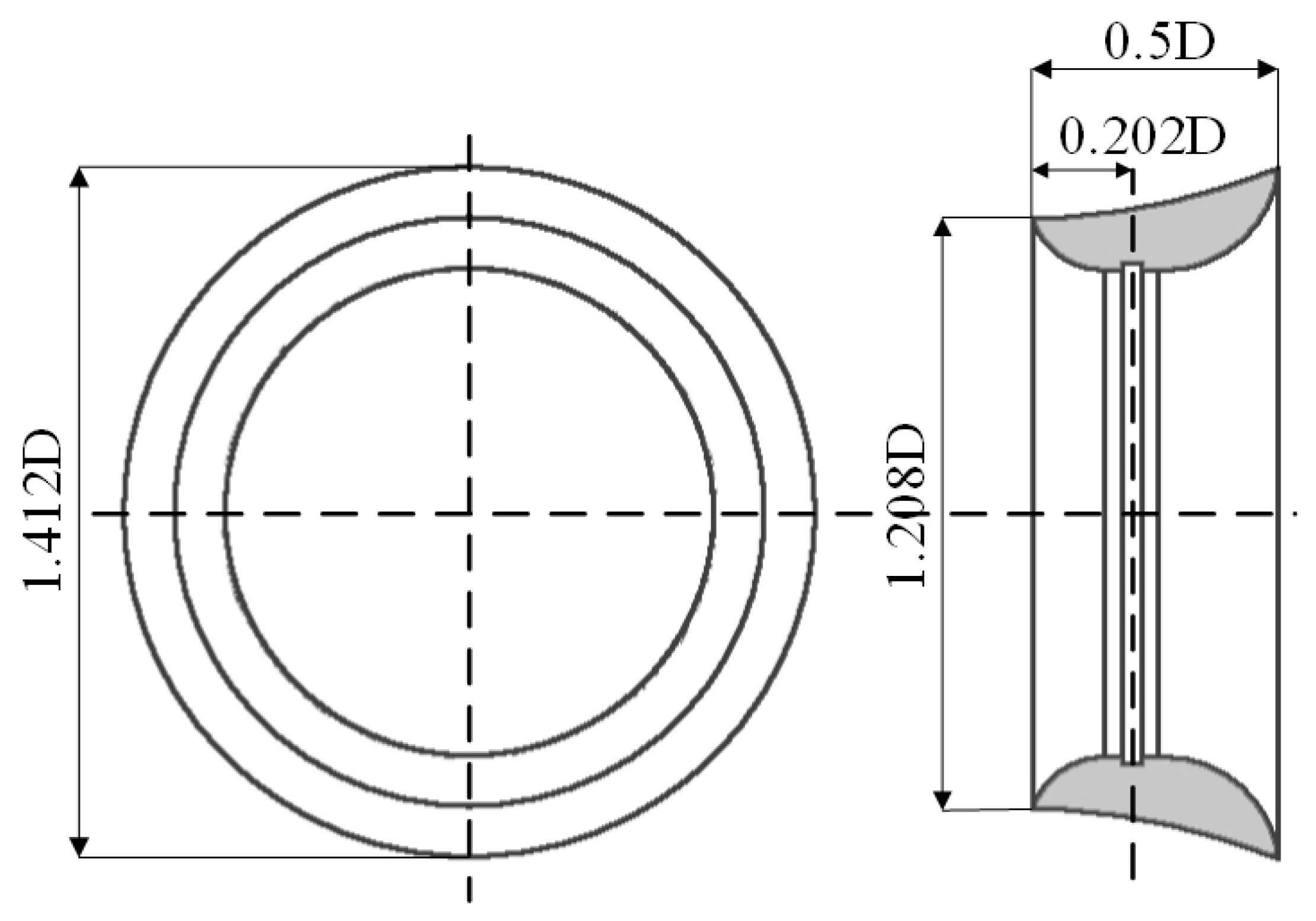
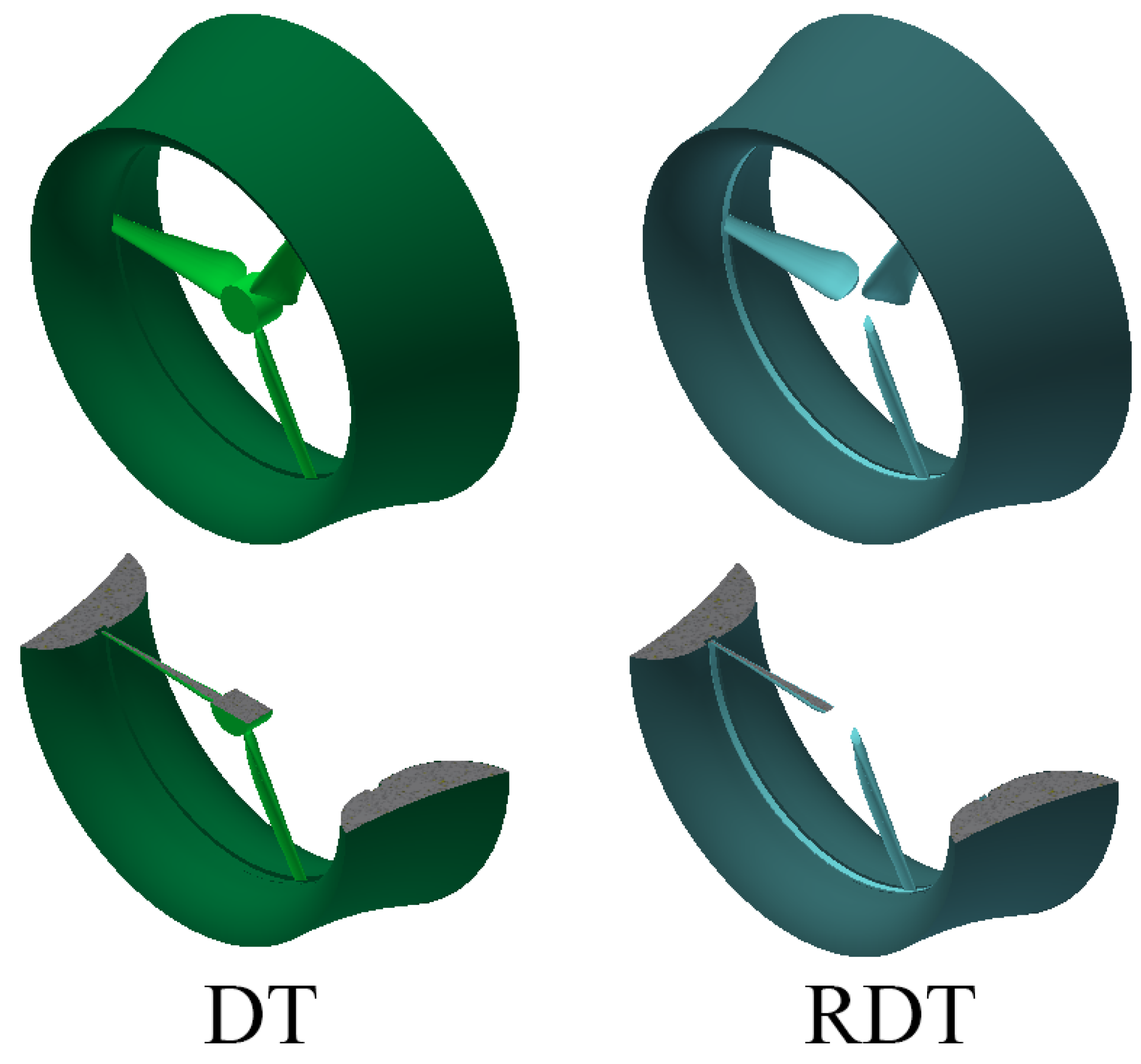
The ANSYS Fluent software (Ansys Inc., Canonsburg, PA, USA) was used to resolve the flow hydrodynamics by solving the Reynolds Averaging Navier-Stokes (RANS) equations via the finite-volume method, which can be written as:
u i x i = 0
t ρ u i + x j ρ u i u j = p x i + x j μ u i x j ρ u i u j ¯ + f i
where u i represents time averaged velocity, p is time average pressure, ρ is fluid density, f i is body force.
The hydrodynamic characteristics of a tidal turbine are often described by the non-dimensional coefficients, including tip speed ratio ( T S R ), power coefficient ( C P ), and thrust coefficient ( C T ), which can be computed, respectively, as follows:
T S R = π n R 30 V 0
C P = P 0.5 ρ A V 0 3
C T = T 0.5 ρ A V 0 2
where P represents the power output ( W ), T represents the turbine thrust ( N ), V 0 represents the incoming flow velocity ( m / s ), n represents the turbine angular velocity ( rpm ), and A represents the area of a reference surface ( m 2 ), R is the radius of turbine ( m ).

2.2. Turbine Model

The three-blade rotor with a diameter (D) of 2 m and hub diameter ratio of 0.1 is used in this study. The “DT08XX” hydrofoils were applied to the rotor, the optimum condition of the rotor is around T S R = 4.0 in axial flow. More rotor characteristics details, like hydrofoils distribution, chord length, twist angle etc, can be found in the reference [30]. The duct has an annular inner groove, in which the groove width is 0.04 D and the groove depth is 0.014 D. The dimension diagram of the duct is shown in Figure 2. The DT contains the duct and the rotor, in which the blade tip is just at the notch of inner groove. The same structural and dimensional configurations are kept for the RDT, except with the hub removed, and the blade tips have connected to the rim. The section size of the rim is slightly smaller than the inner groove so that the rim can be embedded into the annular groove. The schematic view is shown in Figure 3.

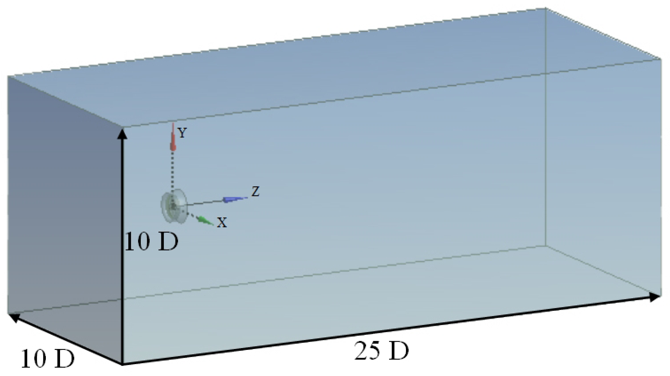
2.3. Computational Domain

As shown in Figure 4, the coordinate system is defined as z in the streamwise, y in the vertical and x in the spanwise directions, respectively. The calculation domain is divided into two sub-domains, an external stationary domain and an internal rotatory domain. The rotatory domain is used to define the rotation of the turbine rotor relative to the stationary domain, thereby, a relative slip between the interfaces and the flow field information is transmitted. The origin of the coordinate system is located in the turbine center. Considering the vastness of the ocean area, the stationary domain should be divided large enough to reduce the influence of the boundary on the calculation accuracy. The turbine is located located 5 D from the inlet and 20 D from the outlet. Taking the maximum cross-sectional area of the duct as the reference area, the blockage ratio of turbine/inlet is less than 1.6%. The interfaces between the rotatory and stationary domains were kept to a minimum by shaping the rotatory domain as a cylinder.

2.4. Boundary Conditions

The tidal current data [31] in the Zhaitang Island tidal current test field (35.613° N, 119.936° E) of China East Sea as shown in Figure 5, was used in this work. The surface wave parameters in the area are 0.6 m in wave height and 3.2 s in wave period. The water shear rate is about 0.002 when depth (H) is between 0 m and 15 m as shown in Figure 6. The velocity inlet was set to 1.56 ± 0.002 H[m/s], accordingly. The two configurations are placed with the turbine centre immersion of 1 D from the surface. Air is assumed to occupy the space above the water, and the surface waves were generated by imposing a boundary condition at the inlet. The free surface elevation and corresponding flow velocity across the water body are computed according to the linear wave theory. Due to the blockage ratio of turbine/inlet is less than 1.6%, the two channel sides have little impact on the turbine hydrodynamics, which were set as free-slip walls. The bed was set as non-slip walls. The top of the channel was set as an open-air boundary condition where the pressure was atmospheric. The outlet was set as a pressure outlet. The SST k ω turbulence model [32] is adopted in the present study to simulate turbulence generation and dissipation.

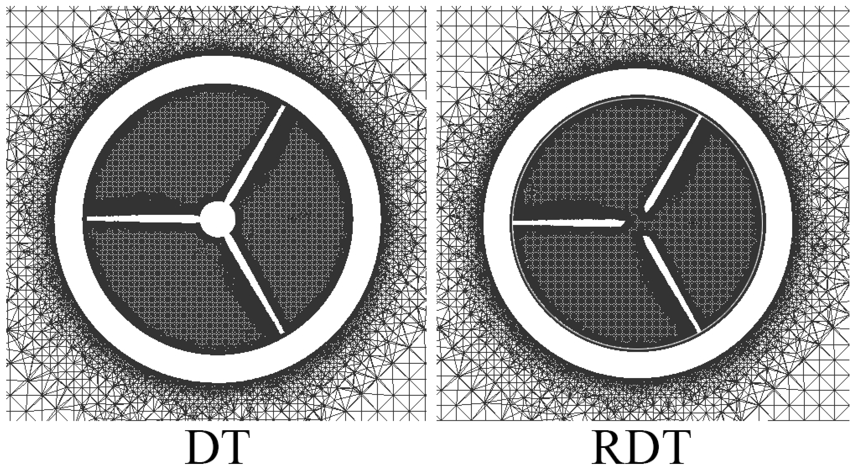
2.5. Mesh Generation

The mesh is generated with an unstructured mesh. As the turbine blade is complex and the tip is too sharp, the grid size of the rotatory domain close to the blade needs to be set smaller, and the surface grid of the blade is further refined, which meets the requirements of the SST k ω turbulence model. Assuming incoming velocity is 1.56 m/s and a reference length is equal to the rotor diameter, the Reynolds number is about 3.1 × 10⁶. The prism layers are placed on the rotor and duct surface with smooth transition normal to the walls. The first layer height satisfies y + = 1 condition and 10 prism layers are placed. The mesh detail on the DT and RDT are shown in Figure 7. A mesh independence assessment of three sets of meshes on RDT at 1.56 m/s and T S R = 4.0 is shown in Table 1, which is carried out by analyzing C P and C T . With the refinement of the mesh, the deviation becomes much smaller. The set of 8.5 million is selected for the subsequent calculations due to the consideration of calculation accuracy and efficiency.

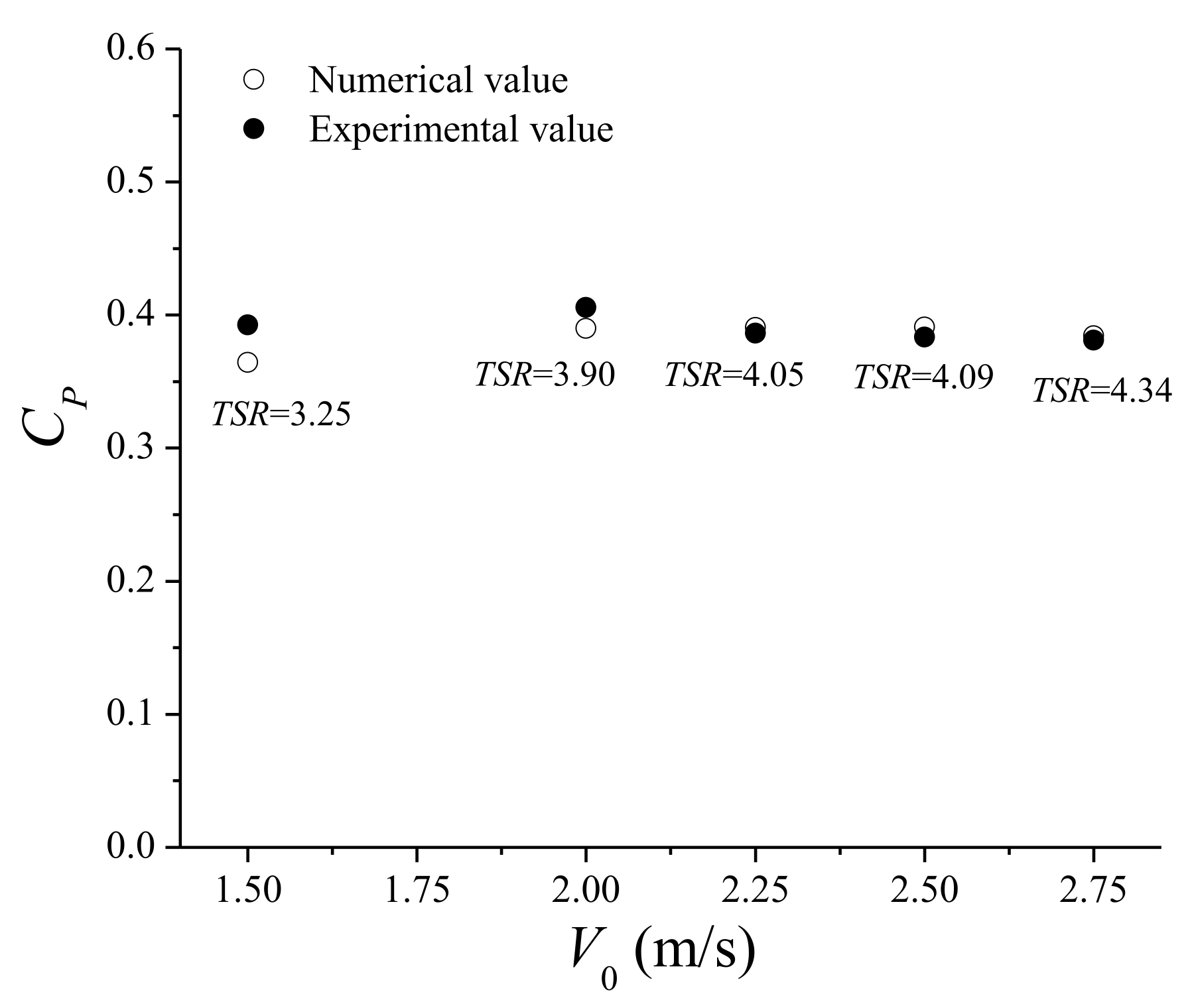
2.6. Numerical Model Validation

To assure reliable results, the present three-blade rotor model was validated by comparison with the experimental value reported in [30] as shown in Figure 8. There is a certain deviation between the numerical value and experimental value. This could be attributed to the following reasons: numerical simulation of a turbine flow field cannot be synchronized due to the fluctuation of environmental factors, for example, temperature, density and current velocity. Numerical simulation assumes a fully turbulent boundary layer, which may not be the case on certain parts of the turbine surface. Besides, Numerical simulation neglects any turbine mechanical structure factors, such as mechanical friction. However, the deviation is within the acceptable range, the numerical value is in good agreement with the experimental value, which indicates that the current simulations have good accuracy and reasonable results.

3. Results and Discussion

In this section, the results and analysis for the axial flow cases and the yawed flow cases of the two configurations are presented, in which the incoming flow moves along the turbines’ axial direction for the axial flow cases, and the yaw angle γ is defined as the angle between the flow direction and the axial direction of the turbine for the yawed flow cases.

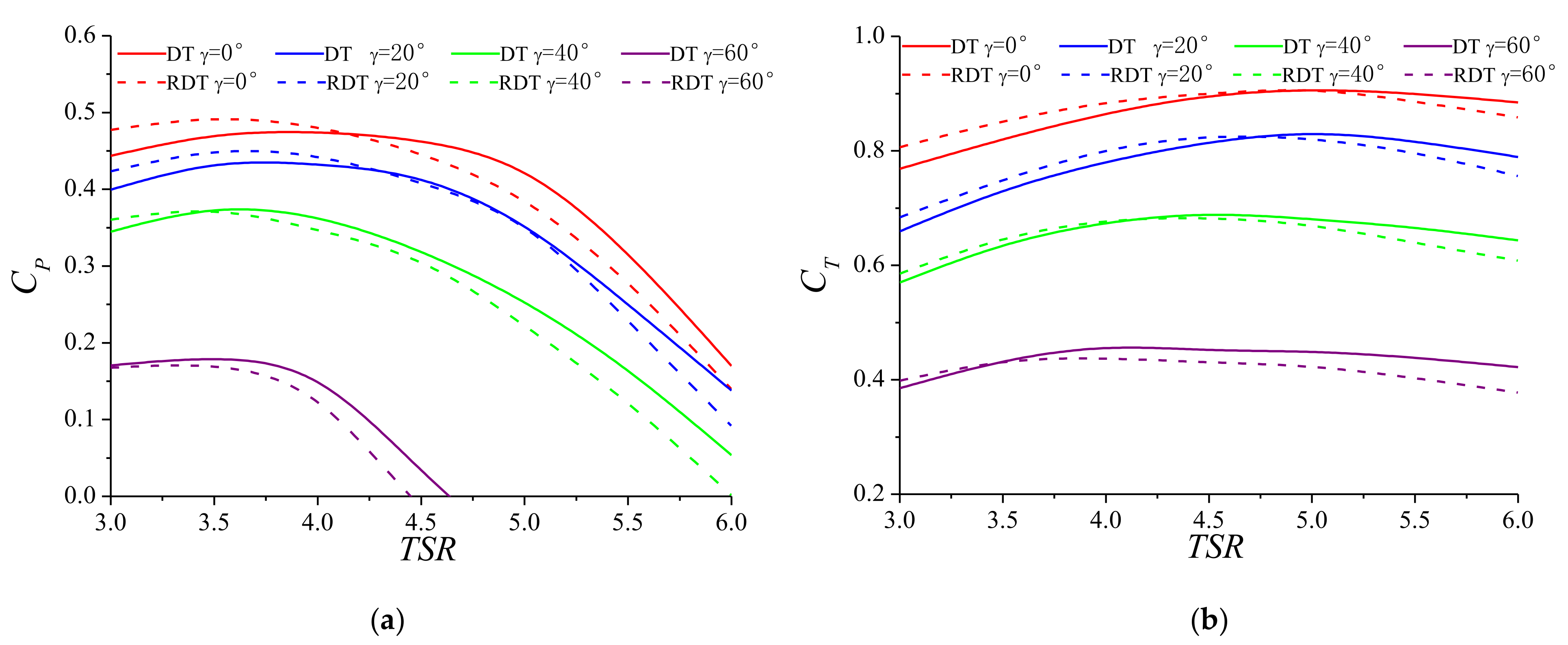
3.1. Power and Thrust

The C P and C T versus T S R at different γ for the configurations is shown in Figure 9. For the axial flow cases, the C P and C T of the two configurations firstly increase, and reach a maximum, then decrease with the increase of T S R . Most interestingly, the RDT features a higher C P level when at 3.0 < T S R < 4.0 with respect to the DT, which indicates the RDT is suitable for operating at lower T S R . It is also noted that the C P of RDT will increase by a magnitude of 1.2346 if reference area is based on the real swept area. On the other hand, the C T of the RDT is slightly higher than that of the DT when at 3.0 < T S R < 5.0. The C P and C T differences for the two configurations is mainly caused by the structural differences between the DT and the RDT. The open-center of RDT permits the undisturbed free stream to flow through it, which causes the different momentum and load values acting on each blade as discussed later. It is worth mentioning that the RDT may have much lower C T and disturbance than the DT in real flow conditions. As mentioned above, the electromagnetic system equipment is integrated inside the duct as a whole structure, and no extra supports and external power generation equipment are required. In summary, the RDT shows potential advantages at energy utilization ratio, drag reduction and structural life within a certain operation range. For the axial flow cases, a notable outcome was the decrease in C P and C T with respect to the axial flow cases. The reduction in yawed flow has two main reasons: first, yawed flow changes the distribution of the relative attack angle of the turbine blade, makes the turbine blade operate away from the optimum angle of attack, and reduces the hydrodynamic performance. The larger the γ is, the farther the turbine blade is from the optimum angle of attack and the more C P and C T is reduced. And second, yawed flow decreases the flow direction projected swept area of the turbine rotation plane, which is also a determinant factor for the C P and C T reduction. The incoming flow passes through the turbine rotation plane and the momentum divides into two components, a streamwise momentum and a spanwise momentum. The former contributes to the lift and torque of the turbine blade. With the increase of γ , the streamwise momentum gets smaller and leads to smaller lift and torque. For the DT, the C P max decreases 8.9%, 21.5% and 62.2% at γ = 20°, 40° and 60° compared with axial flow, respectively. The corresponding C T decreases 10.2%, 27.9% and 50.0% at γ = 20°, 40° and 60° compared with axial flow, respectively. For the RDT, the C P max decreases 8.8%, 24.4% and 65.6% at γ = 20°, 40° and 60° compared with axial flow, respectively. The corresponding C T decreases 12.6%, 25.4% and 49.4% at γ = 20°, 40° and 60° compared with axial flow, respectively. Besides, the yawed flow also affects the variation of the C P and C T curve of both turbines. The maximum T S R point was shifted to lower T S R position with the increase of γ .
Another interest aspect is related to the turbine fatigue hazard. Many tidal turbines fail due to blending. The responsible stresses are cyclic and thus promote fatigue, and a dimensional parameter related to the fatigue damage is C T . According to this, a tidal turbine might act in an optimum condition of performance ( S C P max ), while it is possible to be exposed to the fatigue hazard due to extreme thrust loading and low thickness. To this end, the parameter S C P max [33], represents the superiority of the C P max .
S C P max = C P max C T × % t
where % t represents the maximum thickness of the blade as percentage of the chord length.
Based on 22% thickness (maximum thickness of the blades), the S C P max corresponding to the DT and the RDT is shown in Table 2. It can be observed that the RDT presents a higher S C P max at small γ , and yet has lower S C P max than the DT at large γ .

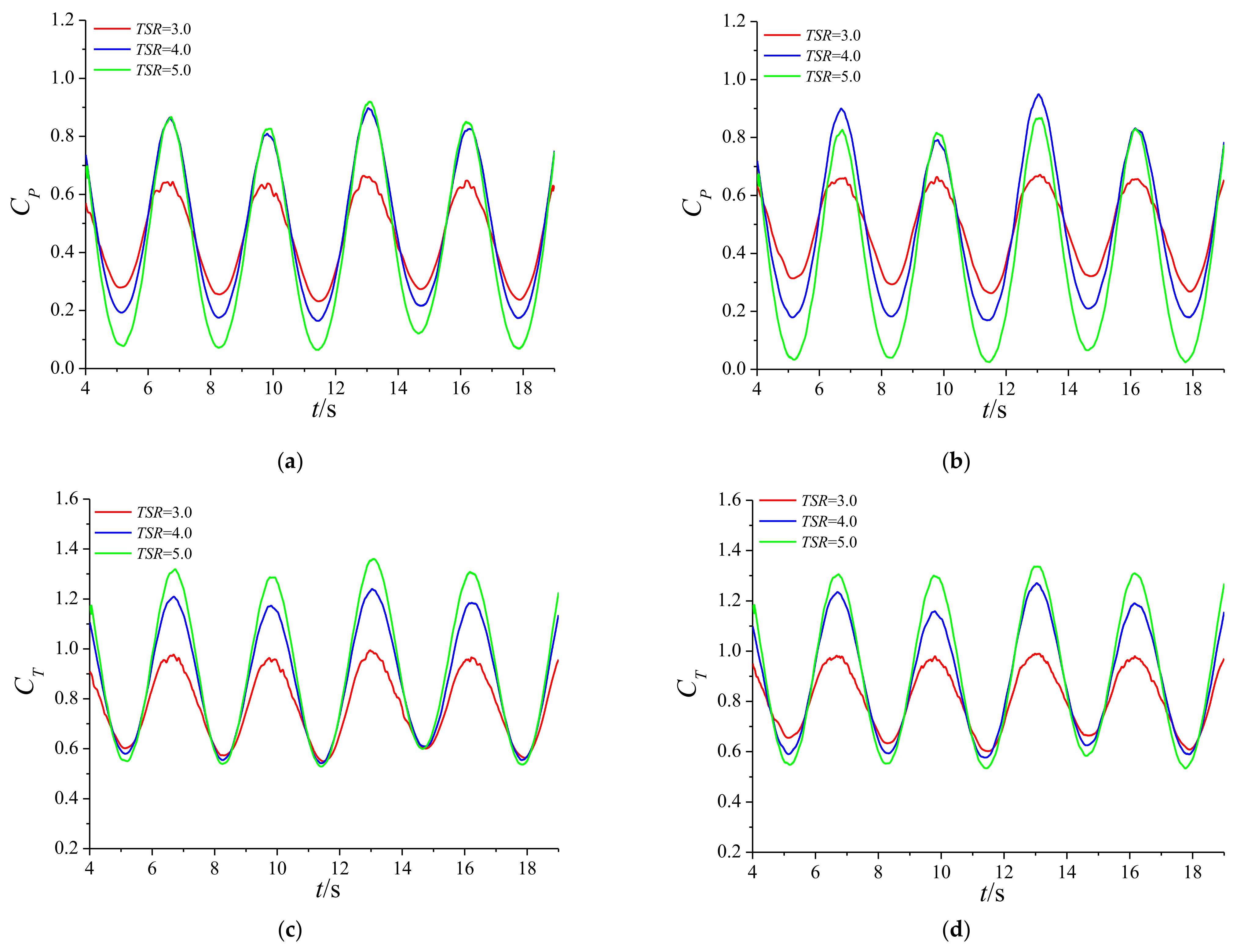
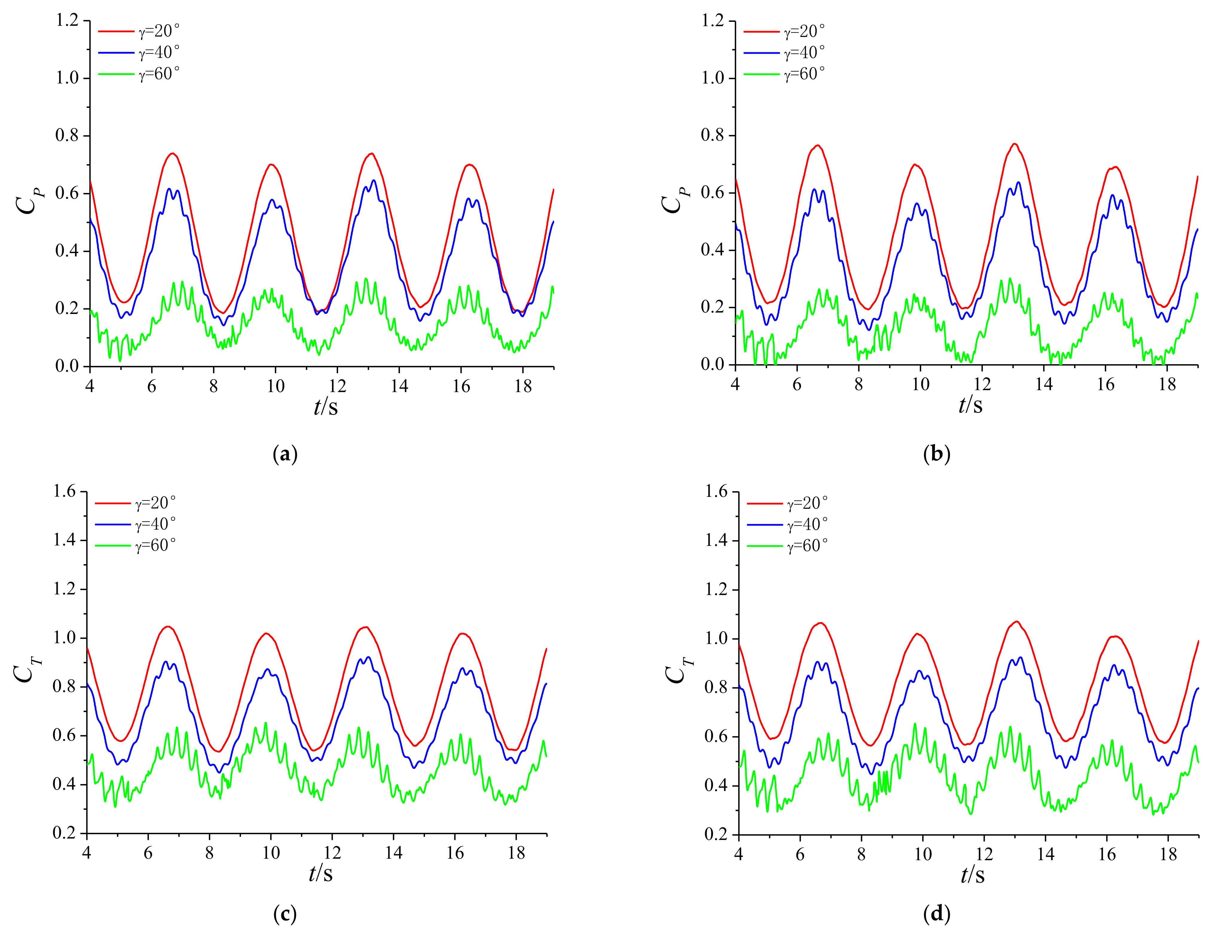
3.2. Performance Fluctuation Characteristics

Taking the axial flow cases at T S R = 3.0, 4.0 and 5.0 as examples, Figure 10 demonstrates the time histories of C P and C T for the two configurations. It can be observed the C P and C T exhibit time-periodic behavior that is consistent with the wave frequency, and there are repeating patterns occurring over a number of wave cycles shown in the Figures. Under the combined wave and current condition, the velocity distribution near the turbines obviously changed. When a wave crest passes through the turbine central x-y plane, the surrounding flow accelerates rapidly, the maximum power and thrust are produced, and the minimum power and thrust occurs when the wave trough passes through the turbine central x-y plane. Meanwhile, and the fluctuation amplitude of the two configurations increase as T S R increases. At T S R = 3.0, the fluctuation amplitude of the two configurations is about 0.22 for C P , and 0.21 for C T . At T S R = 4.0, the fluctuation amplitude of the two configurations is about 0.42 for C P , and 0.36 for C T . At T S R = 5.0, the fluctuation amplitude of the two configurations is about 0.49 for C P , and 0.44 for C T . Thus, the C P fluctuation amplitude at T S R = 4.0 and T S R = 5.0 is 90% and 120% higher than that at T S R = 3.0, respectively, and the C T fluctuation amplitude at T S R = 4.0 and T S R = 5.0 is 70% and 100% higher than that at T S R = 3.0, respectively. With the increase of T S R , the velocity change at the turbine rotation plane is gradually accelerated, and the velocity distribution around the turbine changes constantly. As a result, the bigger the T S R is, the faster the velocity changes, so the larger the amplitude of the change is gradually increased.
Taking the yawed flow cases at T S R = 4.0 and γ = 20°, 40° and 60°as examples, Figure 11 demonstrates the time histories of C P and C T for the two configurations. It can be observed the C P and C T also exhibit time-periodic behavior that is consistent with the wave frequency. Meanwhile, the fluctuation amplitude of the two configurations decreases with the increase of γ . Besides, due to the existence of yawed flow, the C P and C T generates micro-amplitude fluctuation integrated into the main waveform. The frequency of the micro-amplitude fluctuation is consistent with the turbine rotation frequency, and the micro-amplitude fluctuation increases with the increase of γ . The main reason is that the yawed flow changes the relative velocity and amplifies hydrodynamic-non-balance effect of the two configurations during one revolution. It should be noted that the hydrodynamic loads on the turbines will be in a complex form with high frequency and amplitude when the combined wave and yawed flow condition occurs, which is very unfavorable to the stability, safety and reliability of the turbine systems.

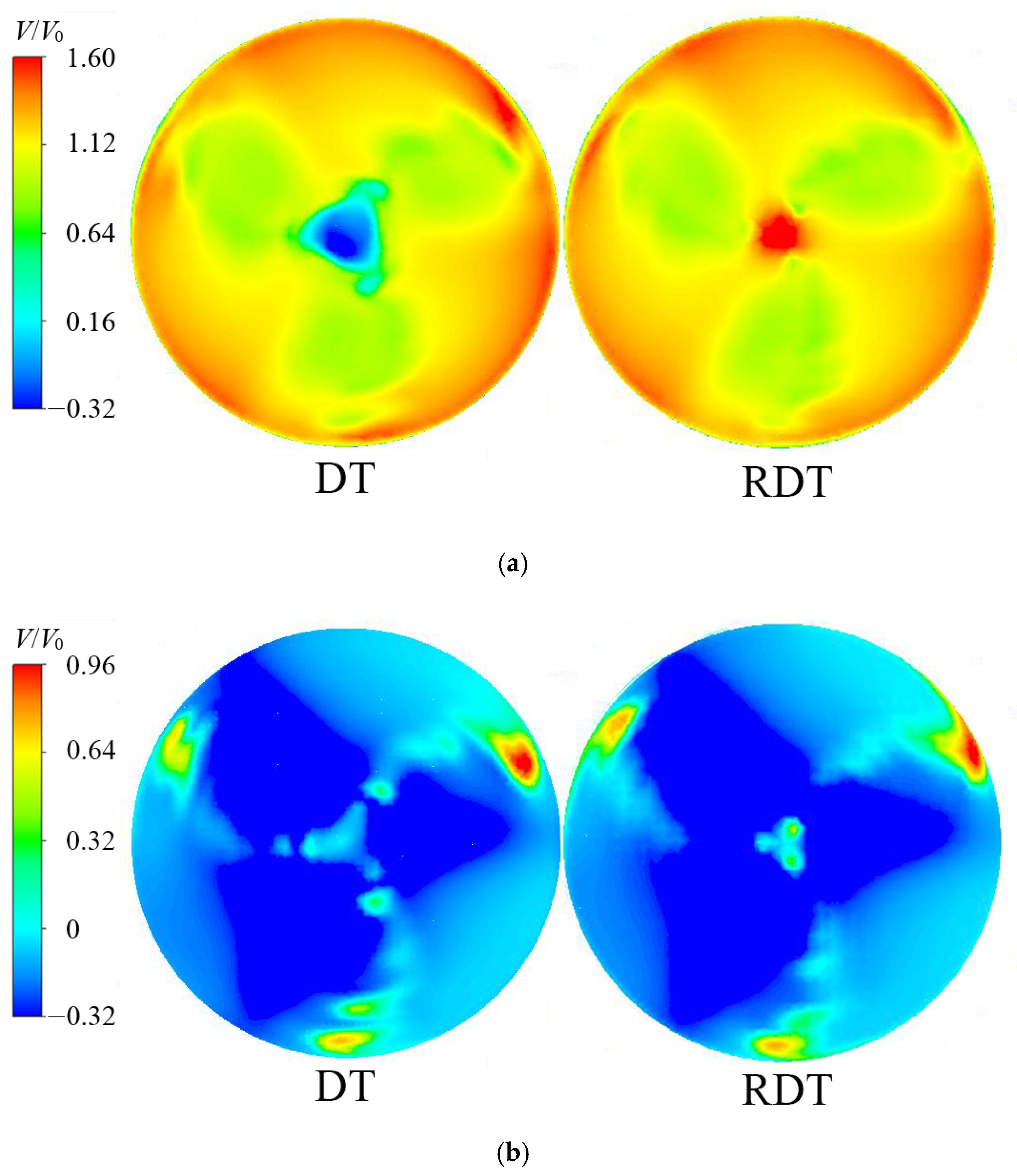
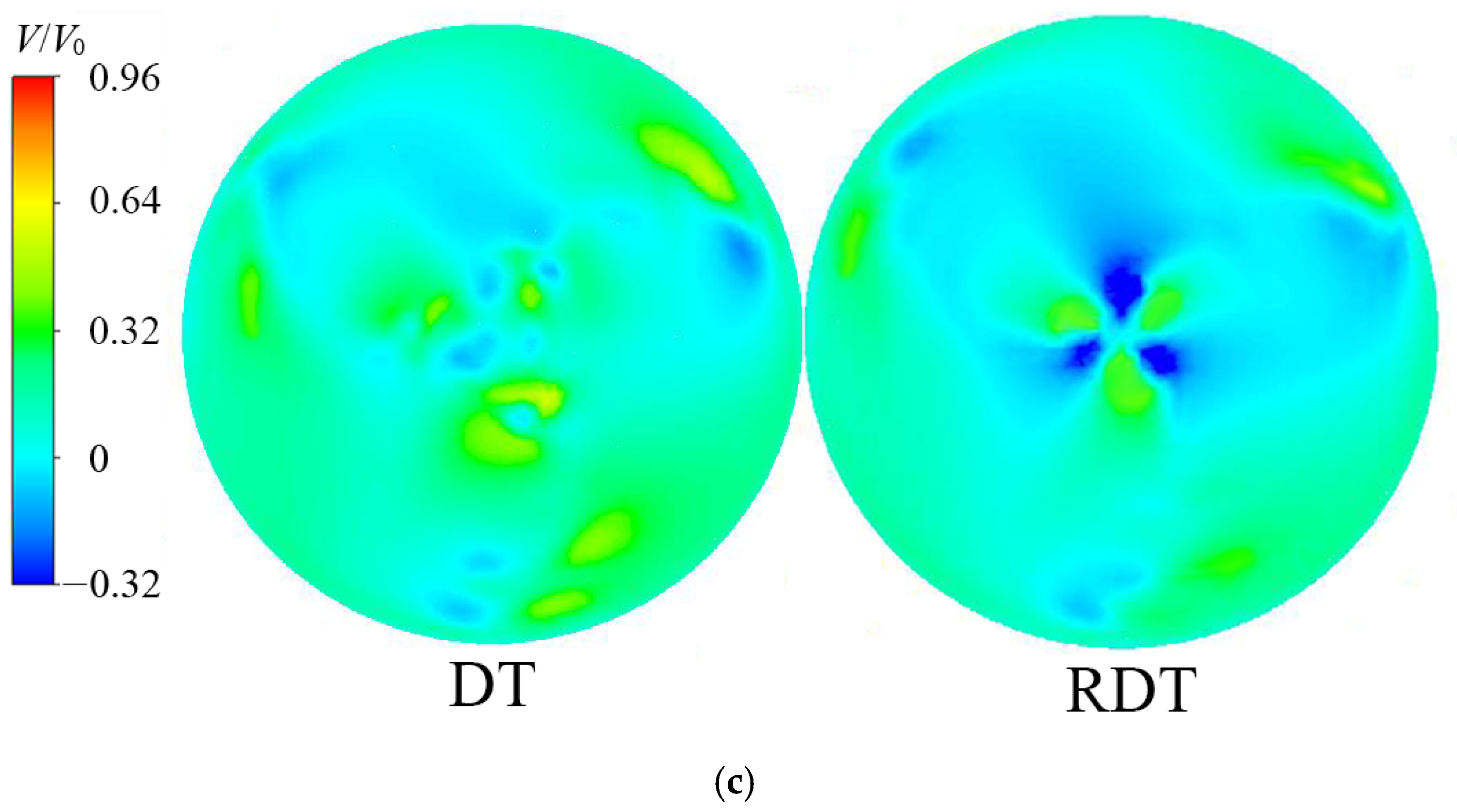
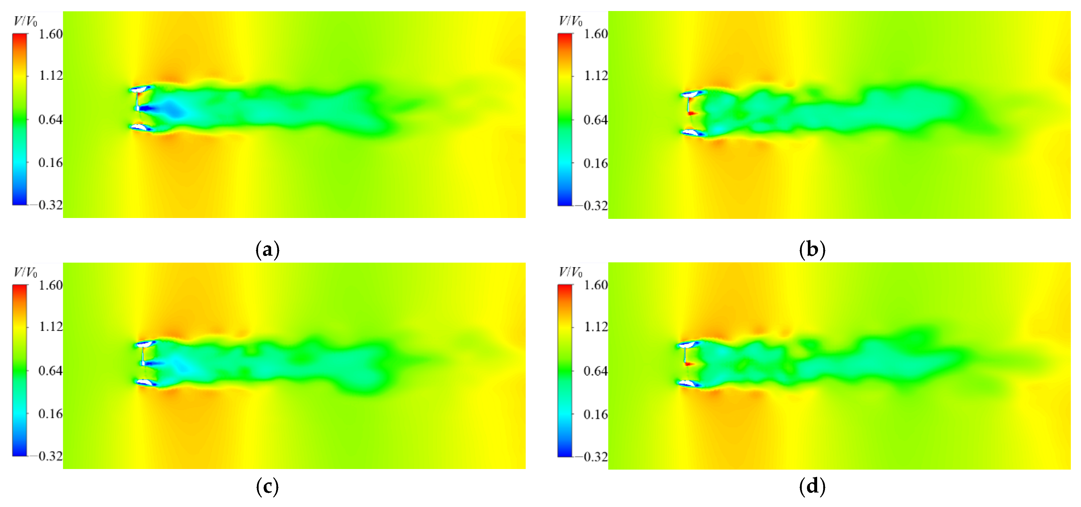
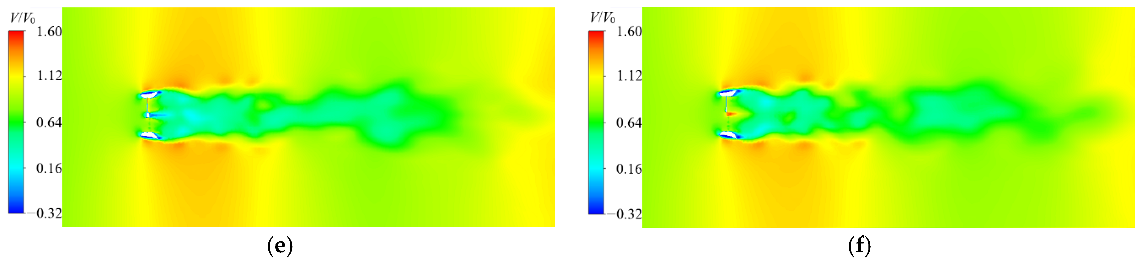
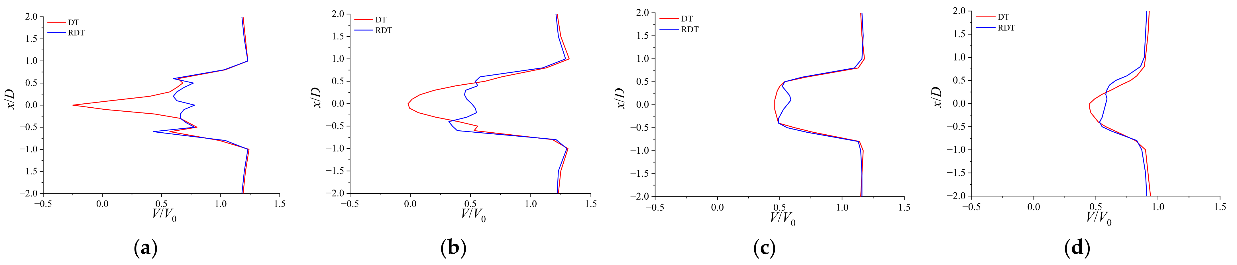
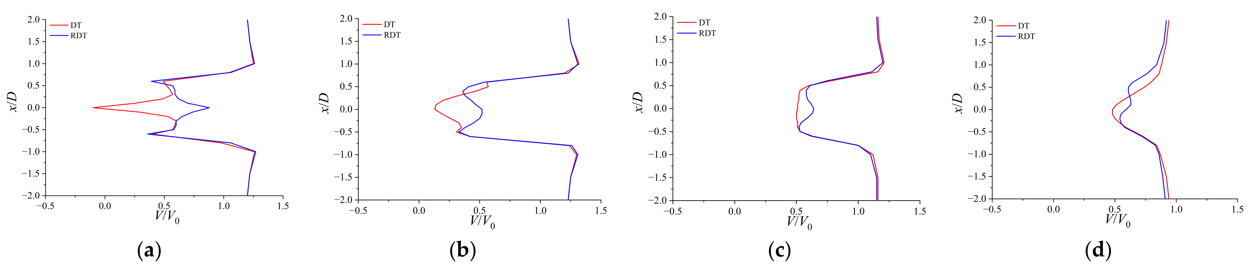
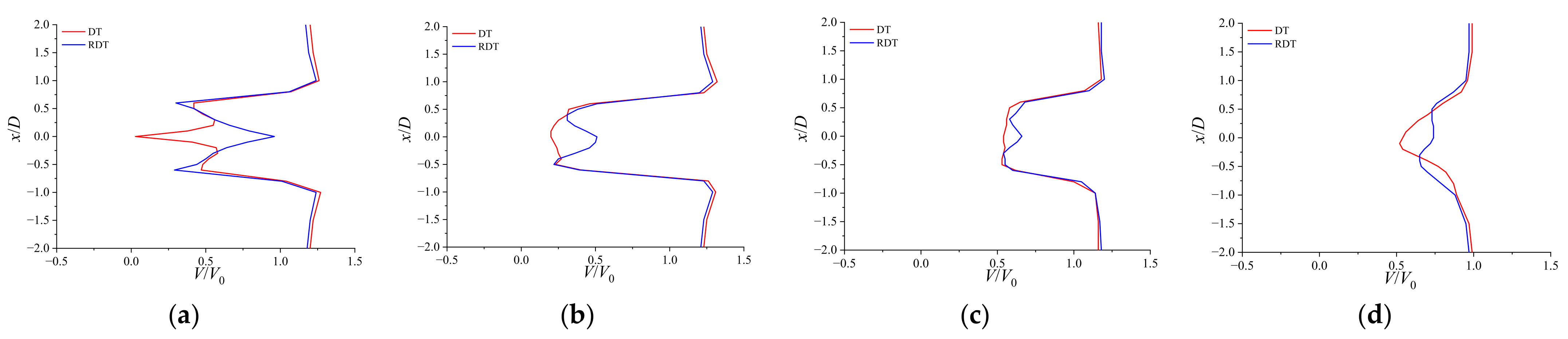
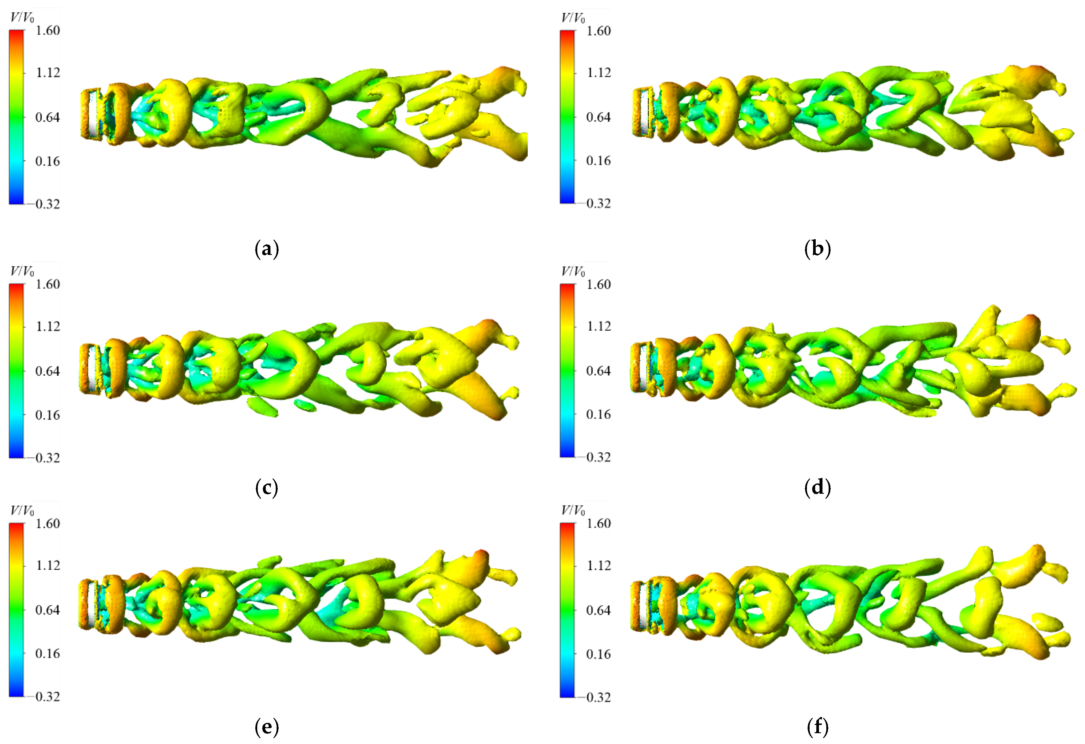
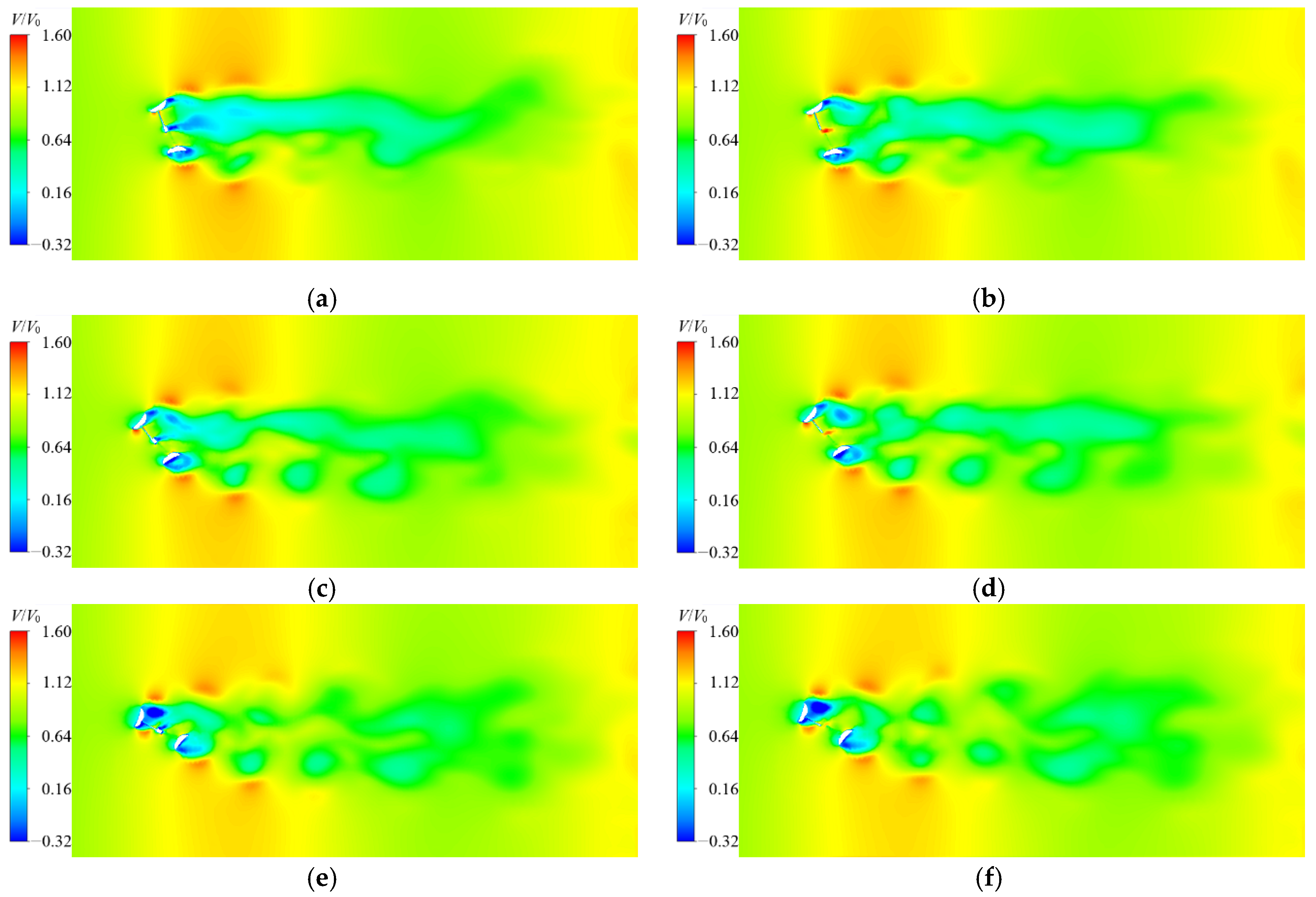
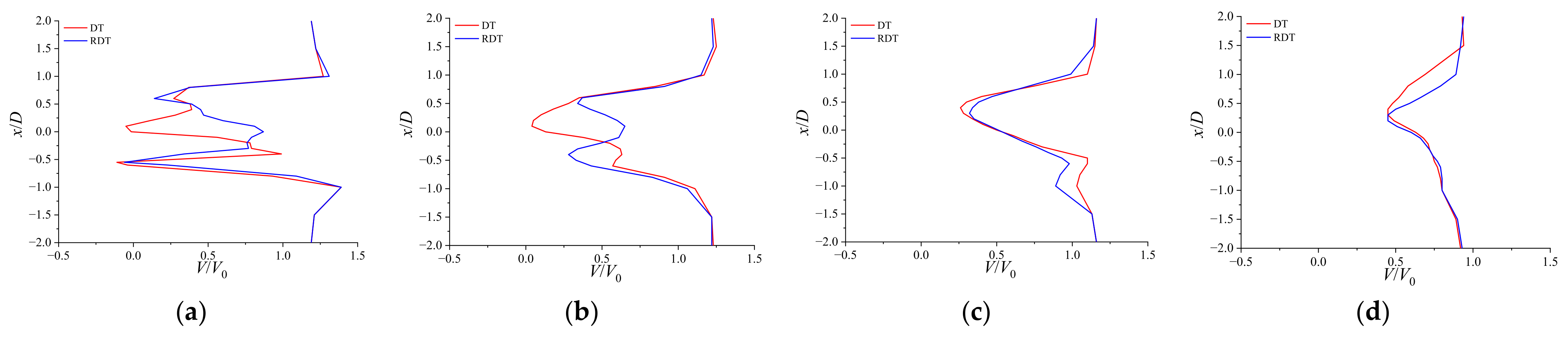
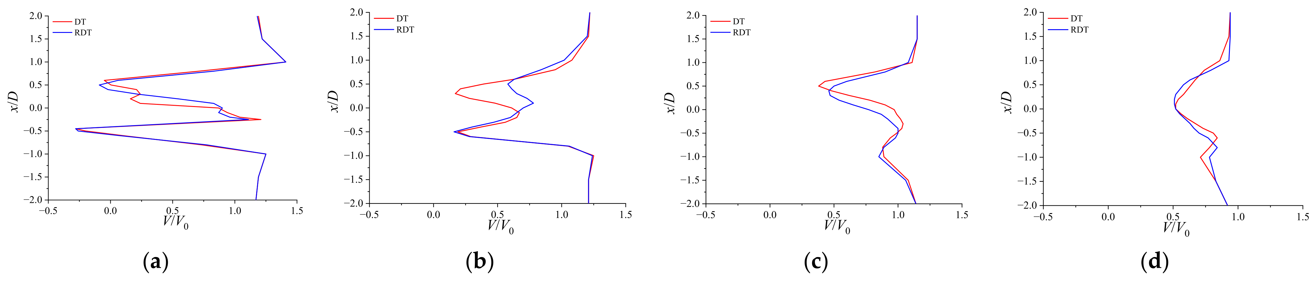
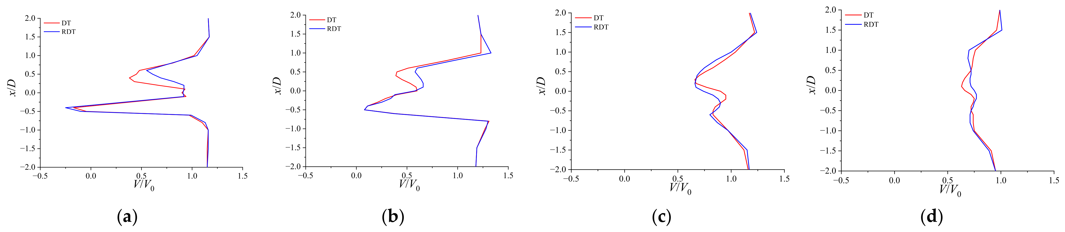
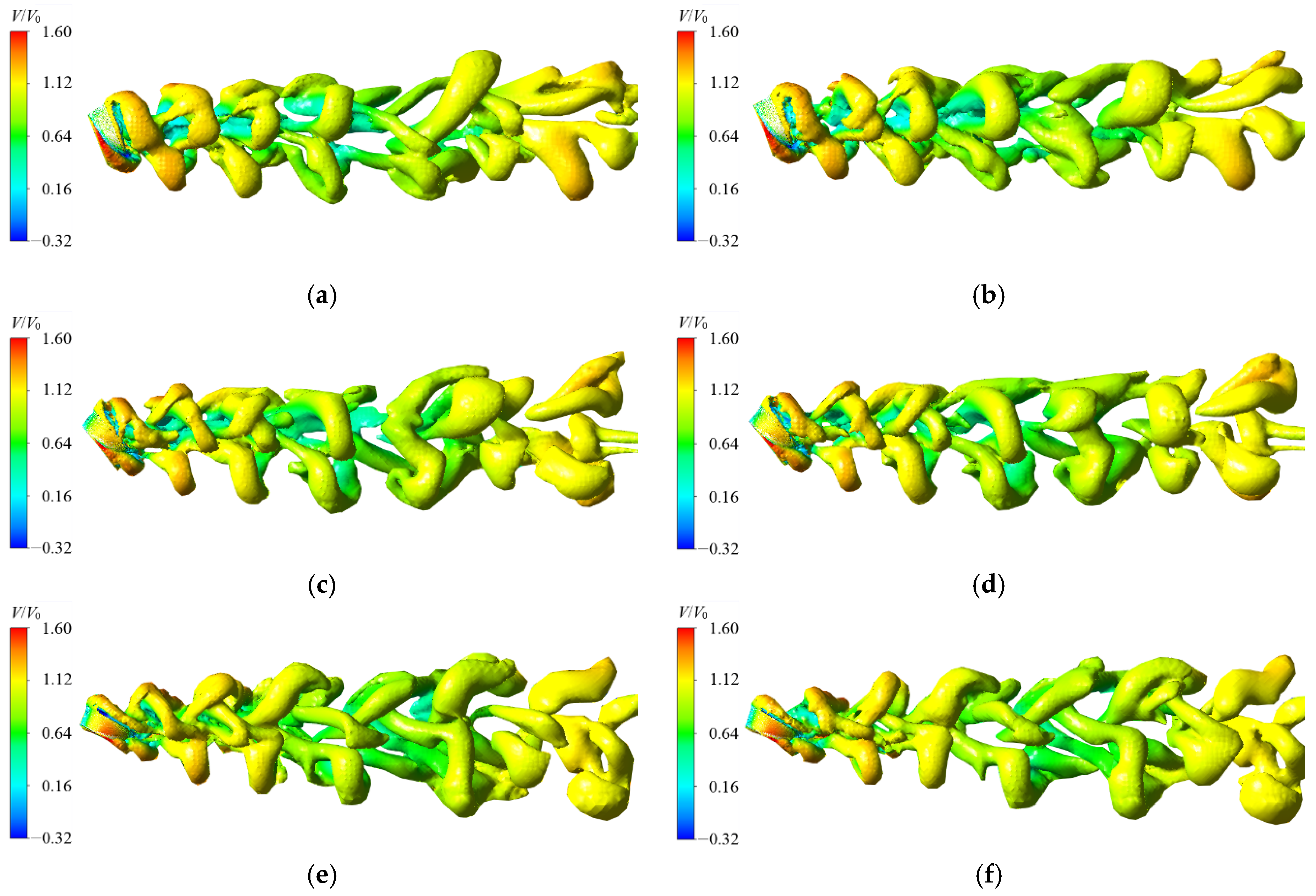
3.3. Wake Characteristics

To illustrate the open-center effect of RDT, the flow analysis was carried out by evaluating the velocity components for the two configurations at T S R = 3.0 in the x-y plane of z/D = 0.1, as shown in Figure 12. For each configuration, a velocity reduction in the axial velocity component behind the turbine, due to the conversion of the kinetic inflow energy into blade mechanical energy, is quite well visible as shown in Figure 12a. For the DT, a flow deceleration is observed at the centre caused by the hub block effect. Due to the RDT does not have a hub, instead, an open-center structure isat the turbine centre. Thus, a part free stream is allowed to travel through the open-center forms an obvious high velocity zone. This causes the different momentum values acting on each blade. The tangential velocity component arises behind the rotor and transforms part of the flow kinetic energy into rotational motion. The tangential velocity component for the two configurations is maximum in proximity of the blade tip, representing, and a source of energy losses for the turbine. However, the intensity near the center is reduced for the RDT owing to the open-center, which recovers this lost power as shown in Figure 12b. Figure 12c shows the radial velocity component for the two configurations. Similarly as the tangential component, the radial velocity component is maximum in proximity of the blade tip. The intensity near the center is also reduced for the RDT, which contributes to recover the radial components. In summary, owing to the open-center, part of energy in the tangential and radial components is recovered for the RDT, enhancing, therefore, the efficiency in the power extraction.
The axial velocity contours for the two configurations at different T S R in the central x-z plane is shown in Figure 13. It is seen that the velocity distribution varies significantly in accordance to certain regions of the wake, and flow downstream for the two configurations are at reduced velocity compared with the free-stream flow of surrounding area. For the DT, there are obvious low velocity zones located behind the hub and trailing edge of duct along the flow direction, which is caused by the blockage effects of the hub and duct. For the RDT, the low velocity zones are primarily located behind the trailing edge of duct. In addition, the low velocity zone for the DT gradually becomes smaller with the increase of T S R , and the high velocity zone for the RDT gradually becomes bigger with the increase of T S R . When a rotor rotates faster, the blockage effect of rotor increases, particularly, when combined with the presence of duct, dramatically increases the blockage effect. Meanwhile, the enhanced blockage effect forces more fluid go through the region near the rotor center at higher T S R , which explain the above phenomenon.
The mean streamwise velocity profiles for the two configurations at different T S R in the central x-z plane are plot in Figure 14, Figure 15 and Figure 16 to quantitatively see how the wake flow develops. Overall, the wake is basically symmetric about x/D = 0, and shows a consistent recovery trend as the flow travels downstream. It can be observed that the DT’s wake profiles show a counterclockwise “W” shaped distribution and the RDT’s show a counterclockwise “V” shaped distribution. Thus, around x/D = 0 and for every T S R , the RDT’s wake has higher velocity than the DT’s. Meanwhile, the value around x/D = 0 for the two configurations increases with the increase of T S R . These velocity distributions are consistent with the results as discussed in Figure 13. Besides, there is always a local minimum of velocity around x/D = ±0.6 (duct position) for the two configurations at z/D = 0.5, which is caused by the blockage effect. The local minimum increases as downstream distance increases, suggesting an increasing recovery. Overall, the presence of open-center of RDT has avoided the low velocity zone, improved the wake structure and accelerated wakes recover, which gives an advantageous effect in operating a RDT.
For better understanding the flow characteristics at different T S R , the vortex structures for the two configurations at different T S R is shown in Figure 17, which are plotted using Iso-surfaces of instantaneous colored by the streamwise velocity. It can be observed that the vortex structures of the two configurations have similar shapes at same T S R . The blade tips vortices have mixed duct’s vortices and shed from the trailing edge of duct like crossed spiral lines, with a diameter slightly larger than that of the rotor. In addition, small vortexes are observed at the leading edge of duct for the two configurations, as indicated by the contours.
The axial velocity contours for the two configurations at T S R = 4.0 and different γ in the central x-z plane is shown in Figure 18. Obviously, the yawed flow has made the wakes asymmetric about the flow direction. The γ primarily determines the downstream wake deflection direction and significantly changes the wake shape. The yawed flow field is more turbulent than the axial flow field, and the two configurations suffer strong unsteady flow separation along the whole span. As can be seen in the Figures, slight flow separation occurred at γ = 20°. As γ increases, the angle of attack of the duct’s upper portion decreases and the angle of attack of the duct’s lower portion increases, which has led to significant flow separation and blockage effects around the duct’s upper trailing edge and duct’s lower leading edge for the two configuration. Meanwhile, strong interactions are observed between the rotor’s main wake and the duct’s upper wake. The duct’s upper trailing edge cause larger flow separations than the duct’s lower leading edge, which is response for the present asymmetric shapes of the wakes. Besides, the sizes of main wake’s low velocity zones decrease with the increase of γ , resulting in weaker wake vortex. Of course, the rotor rotation motions add more complexities to the flow felid and make the wake more unstable. Overall, the structures of the wake, including the main wake, flow separation zones caused by duct, are almost the same for the two configurations at same γ , except for the local area near the turbine axis in which a part free-stream flow still can travel through the open-center of the RDT. In addition, the sizes of low velocity zones for the DT or the size of high velocity zones for the RDT decrease with the increase of γ .
The mean streamwise velocity profiles for the two configurations at T S R = 4.0 and different γ in the central x-z plane are plot in Figure 19, Figure 20 and Figure 21. From the profiles, the wake is asymmetric about x/D = 0, especially at z/D = 0.5 and 1.0. Affected by yawed flow, there are two main minimum of velocity around x/D = ±0.6 for the two configurations at z/D = 0.5, which is caused by the blockage effect of deflected duct. As γ increases, the upper minimum value increases and the lower minimum value decreases, and the wakes recover faster.
To more clearly visualize the impact that yawed flow has on the flow characteristics, the vortex structures for the two configurations at T S R = 4.0 and different γ is shown in Figure 22, which are plotted using Iso-surfaces of instantaneous colored by the streamwise velocity. The vortex structures of the two configurations have similar shapes at same γ . Compared with the results in Figure 17, the vortex structures changes significantly, and almost the entire surface of the duct suffers from flow separation. The presence of the duct has made the flow field more turbulent, which weakens the main vortices shed from blade tips [34] and enhanced the vortices from the duct’s upper trailing edge and duct’s lower leading edge with the increase of γ , which is consistent with the results as discussed in Figure 18.

4. Conclusions

In the present study, computational fluid dynamics simulations were performed to show the performance between a RDT and the corresponding DT in real flow based on the Zhaitang Island’s tidal current data, including the variation of power, thrust, and wake characteristics. Important results of this research are as follows:
Under axial flow conditions, the C P and C T exhibit time-periodic behavior that is consistent with the wave frequency. Meanwhile, the fluctuation amplitude increase with the increase of T S R . The bigger the T S R is, the faster the velocity changes, so the larger the amplitude of the change is gradually increased. The RDT features a higher C P level when at 3.0 < T S R <4.0 with respect to the DT, which indicates the RDT is suitable for operating at lower T S R . It is also noted that the C P of RDT will increase by a magnitude of 1.2346 if reference area is based on the real swept area. Although, the C T of the RDT is slightly higher than that of the DT when at 3.0 < T S R < 5.0. The RDT may have much lower C T and disturbance than the DT in real flow conditions. Due to the RDT’s electromagnetic system equipment is integrated inside the duct as a whole structure, no extra supports and external power generation equipment are required. Thus, the RDT shows potential advantages at energy utilization ratio, drag reduction and structural life within a certain operation range. The wake characteristics analysis reveals that the wake of the two configurations is basically symmetric about the flow direction. The blade tips vortices have mixed duct’s vortices and shed from the duct’s trailing edge like crossed spiral lines, with a diameter slightly larger than that of the rotor. Due to the RDT does not have a hub, instead, an open-center structure is at the turbine centre. Thus, a part free-stream flow is allowed to travel through the open-center and forms an obvious high velocity zone. The presence of open-center of RDT has avoided the low velocity zone, improved the wake structure and accelerated wakes recover, which gives an advantageous effect in operating a RDT.
Under yawed flow conditions, the C P and C T still exhibit time-periodic behavior that is consistent with the wave frequency, and the fluctuation amplitude of the two configurations decrease with the increase of γ . Besides, the C P and C T of the two configurations decrease with the increase of γ . On the other hand, due to the existence of yawed flow, the C P and C T generates micro-amplitude fluctuation integrated into the main waveform. The frequency of the micro-amplitude fluctuation is consistent with the turbine rotation frequency, and the micro-amplitude fluctuation increases with the increase of γ . The main reason is that the yawed flow changes the relative velocity and amplifies hydrodynamic-non-balance effect of the two configurations during one revolution. The wake characteristics analysis reveals that the yawed flow has made the wakes asymmetric about the flow direction. The yawed flow field is more turbulent than the axial flow field, and the two configurations suffer strong unsteady flow separation along the whole span. Strong interactions are observed between the rotor’s main wake and the duct’s upper wake. The γ primarily determines the downstream wake deflection direction and significantly changes the wake shape and vortex structures. The presence of the duct has made the flow field more turbulent with the increase of γ , which weakens the main vortices shed from blade tips and enhanced the vortices from the duct’s upper trailing edge and duct’s lower leading edge. In addition, the wake flow is found to recover more quickly at larger γ .

Author Contributions

Conceptualization, K.S.; methodology, K.S. and Y.K.; software, Y.K.; validation, K.S.; formal analysis, K.S.; investigation, K.S.; resources, K.S.; data curation, K.S.; writing—original draft preparation, K.S.; writing—review and editing, K.S.; visualization, Y.K.; supervision, K.S.; project administration, K.S.; funding acquisition, K.S. All authors have read and agreed to the published version of the manuscript.

Funding

This work was supported by the Yunnan Fundamental Research Project (grant no. 202201AU070028) and the Scientific Research Foundation of Kunming University (grant no. YJL20023).

Institutional Review Board Statement

Not applicable.

Informed Consent Statement

Not applicable.

Data Availability Statement

Not applicable.

Conflicts of Interest

The authors declare no conflict of interest.

References

  1. Alotaibi, I.; Abido, M.A.; Khalid, M.; Savkin, A.V. A comprehensive review of recent advances in smart grids: A sustainable future with renewable energy resources. Energies 2020, 13, 6269. [Google Scholar] [CrossRef]
  2. Ellabban, O.; Abu-Rub, H.; Blaabjerg, F. Renewable energy resources: Current status, future prospects and their enabling technology. Renew. Sustain. Energy Rev. 2014, 39, 748–764. [Google Scholar] [CrossRef]
  3. Chen, L.; Li, W.; Li, J.; Fu, Q.; Wang, T. Evolution Trend Research of Global Ocean Power Generation Based on a 45-Year Scientometric Analysis. J. Mar. Sci. Eng. 2021, 9, 218. [Google Scholar] [CrossRef]
  4. Khan, M.J.; Bhuyan, G.; Iqbal, M.T.; Quaicoe, J.E. Hydrokinetic energy conversion systems and assessment of horizontal and vertical axis turbines for river and tidal applications: A technology status review. Appl. Energy 2009, 86, 1823–1835. [Google Scholar] [CrossRef]
  5. Vermaak, H.J.; Kusakana, K.; Koko, S.P. Status of micro-hydrokinetic river technology in rural applications: A review of literature. Renew. Sustain. Energy Rev. 2014, 29, 625–633. [Google Scholar] [CrossRef]
  6. Olczak, A.; Stallard, T.; Feng, T.; Stansby, P.K. Comparison of a rans blade element model for tidal turbine arrays with labor-atory scale measurements of wake velocity and rotor thrust. J. Fluids Struct. 2016, 64, 87–106. [Google Scholar] [CrossRef]
  7. Magagna, D.; Monfardini, R.; Uihlein, A. JRC Ocean Energy Status Report; Publications Office of the European Union: Copenhagen, Denmark, 2016. [Google Scholar]
  8. Nachtane, M.; Tarfaoui, M.; Goda, I.; Rouway, M. A review on the technologies, design considerations and numerical models of tidal current turbines. Renew. Energy 2020, 157, 1274–1288. [Google Scholar] [CrossRef]
  9. Walker, S.; Thies, P.R. A review of component and system reliability in tidal turbine deployments. Renew. Sustain. Energy Rev. 2021, 151, 111495. [Google Scholar] [CrossRef]
  10. Liu, P.; Veitch, B. Design and optimization for strength and integrity of tidal turbine rotor blades. Energy 2012, 46, 393–404. [Google Scholar] [CrossRef]
  11. Zhu, F.W.; Ding, L.; Huang, B.; Bao, M.; Liu, J.T. Blade design and optimization of a horizontal axis tidal turbine. Ocean Eng. 2020, 195, 106652. [Google Scholar] [CrossRef]
  12. Creech, A.C.; Borthwick, A.G.; Ingram, D. Effects of support structures in an LES actuator line model of a tidal turbine with contra-rotating rotors. Energies 2017, 10, 726. [Google Scholar] [CrossRef]
  13. Nan, D.; Shigemitsu, T.; Zhao, S.; Ikebuchi, T.; Takeshima, Y. Study on performance of contra-rotating small hydro-turbine with thinner blade and longer front hub. Renew. Energy 2018, 117, 184–192. [Google Scholar] [CrossRef]
  14. Huang, B.; Zhu, G.J.; Kanemoto, T. Design and performance enhancement of a bi-directional counter-rotating type horizontal axis tidal turbine. Ocean Eng. 2016, 128, 116–123. [Google Scholar] [CrossRef]
  15. Baratchi, F.; Jeans, T.L.; Gerber, A.G. Assessment of blade element actuator disk method for simulations of ducted tidal turbines. Renew. Energy 2020, 154, 290–304. [Google Scholar] [CrossRef]
  16. Allsop, S.; Peyrard, C.; Bousseau, P.; Thies, P. Adapting conventional tools to analyse ducted and open centre tidal stream turbines. Int. Mar. Energy J. 2018, 1, 91–99. [Google Scholar] [CrossRef]
  17. Rezek, T.J.; Camacho, R.; Filho, N.M.; Limacher, E.J. Design of a Hydrokinetic Turbine Diffuser Based on Optimization and Computational Fluid Dynamics. Appl. Ocean Res. 2020, 107, 102484. [Google Scholar] [CrossRef]
  18. Tampier, G.; Troncoso, C.; Zilic, F. Numerical analysis of a diffuser-augmented hydrokinetic turbine. Ocean Eng. 2017, 145, 138–147. [Google Scholar] [CrossRef]
  19. Yan, X.; Liang, X.; Ouyang, W.; Liu, Z.; Liu, B.; Lan, J. A review of progress and applications of ship shaft-less rim-driven thrusters. Ocean Eng. 2017, 144, 142–156. [Google Scholar] [CrossRef]
  20. Gaggero, S. Numerical design of a RIM-driven thruster using a RANS-based optimization approach. Appl. Ocean Res. 2020, 94, 101941. [Google Scholar] [CrossRef]
  21. Dubas, A.J.; Bressloff, N.W.; Sharkh, S.M. Numerical modelling of rotor–stator interaction in rim driven thrusters. Ocean Eng. 2015, 106, 281–288. [Google Scholar] [CrossRef] [Green Version]
  22. Liang, X.; Yan, X.; Ouyang, W.; Liu, Z. Experimental research on tribological and vibration performance of water-lubricated hydrodynamic thrust bearings used in marine shaft-less rim driven thrusters. Wear 2019, 426, 778–791. [Google Scholar] [CrossRef]
  23. Borg, M.G.; Xiao, Q.; Allsop, S.; Incecik, A.; Peyrard, C. A numerical performance analysis of a ducted, high-solidity tidal turbine. Renew. Energy 2020, 159, 663–682. [Google Scholar] [CrossRef]
  24. Borg, M.G.; Xiao, Q.; Allsop, S.; Incecik, A.; Peyrard, C. A numerical structural analysis of ducted, high-solidity, fibre-composite tidal turbine rotor configurations in real flow conditions. Ocean Eng. 2021, 233, 109087. [Google Scholar] [CrossRef]
  25. Song, K.; Yang, B. A Comparative Study on the Hydrodynamic-Energy Loss Characteristics between a Ducted Turbine and a Shaftless Ducted Turbine. J. Mar. Sci. Eng. 2021, 9, 930. [Google Scholar] [CrossRef]
  26. Djebarri, S.; Charpentier, J.F.; Scuiller, F.; Benbouzid, M. Design and performance analysis of double stator axial flux PM generator for rim driven marine current turbines. IEEE J. Ocean. Eng. 2015, 41, 50–66. [Google Scholar]
  27. Djebarri, S.; Charpentier, J.F.; Scuiller, F.; Benbouzid, M. Comparison of direct-drive PM generators for tidal turbines. In Proceedings of the International Power Electronics and Application Conference and Exposition, Shanghai, China, 20–22 November 2014. [Google Scholar]
  28. Feng, B.; Liu, X.; Ying, Y.; Si, Y.; Zhang, D.; Qian, P. Research on the tandem arrangement of the ducted horizontal-axis tidal turbine. Energy Convers. Manag. 2022, 258, 115546. [Google Scholar]
  29. Open Hydro Ltd. Cape Sharp Tidal, Bay of Fundy, Nova Scotia, Canada. Available online: http://www.openhydro.com/Projects (accessed on 1 March 2018).
  30. Song, K.; Wang, W.; Yan, Y. Numerical and experimental analysis of a diffuser-augmented micro-hydro turbine. Ocean Eng. 2018, 171, 590–602. [Google Scholar] [CrossRef]
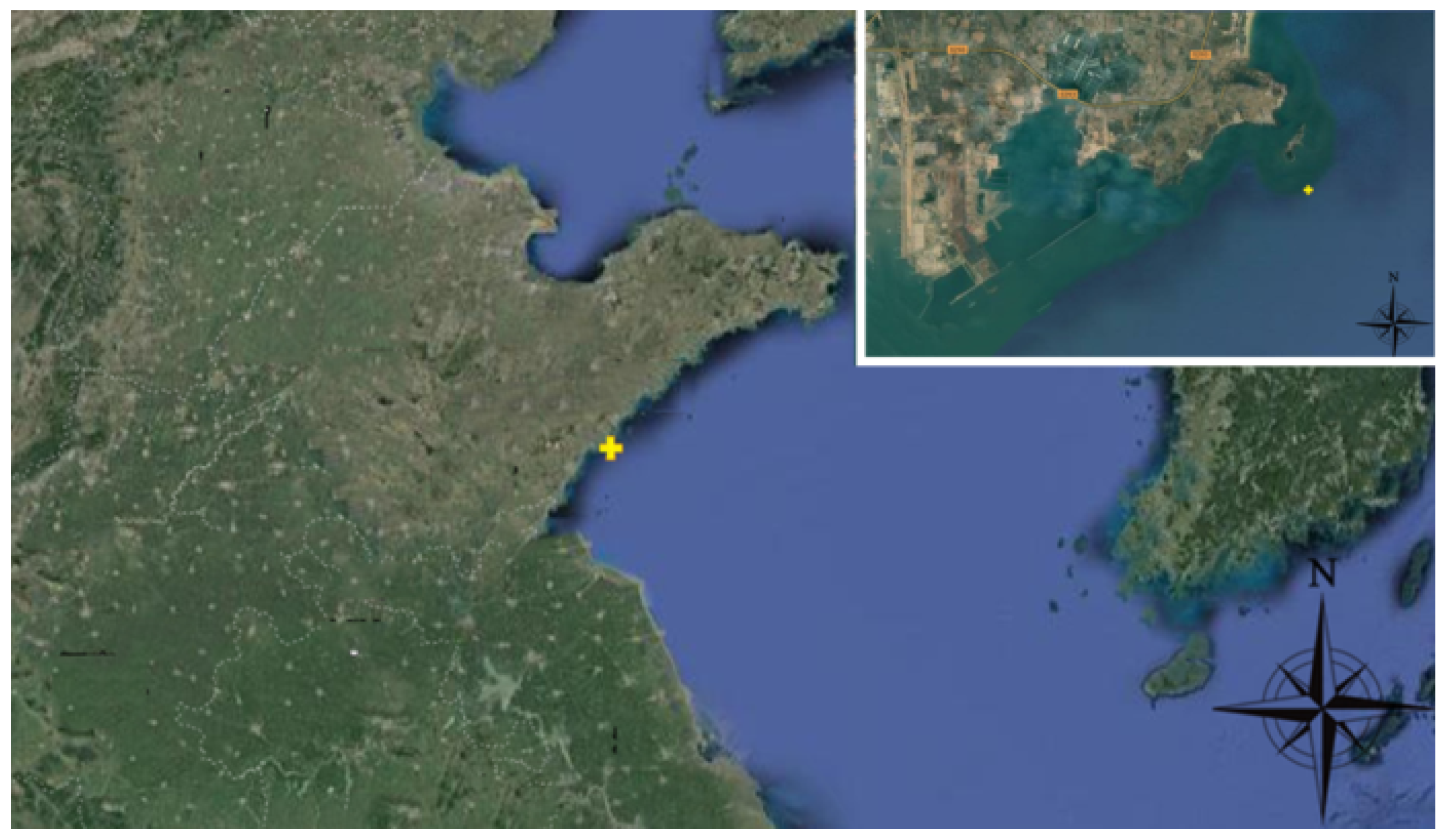
  31. Jiang, X.; Wang, S.; Si, X.; Yuan, P.; Tan, J. Tidal stream characteristic analysis and micro-sitting selection in sea area around Zhaitang island. Acta Energ. Sol. Sin. 2018, 39, 892–899. (In Chinese) [Google Scholar]
  32. Menter, F.R. Two-equation eddy-viscosity turbulence models for engineering applications. AIAA J. 1994, 32, 1598–1605. [Google Scholar] [CrossRef]
  33. Alipour, R.; Alipour, R.; Fardian, F.; Tahan, M.H. Optimum performance of a horizontal axis tidal current turbine: A numerical parametric study and experimental validation. Energy Convers. Manag. 2022, 258, 115533. [Google Scholar] [CrossRef]
  34. Lee, H.; Lee, D.J. Wake impact on aerodynamic characteristics of horizontal axis wind turbine under yawed flow conditions. Renew. Energy 2019, 136, 383–392. [Google Scholar] [CrossRef]
Figure 1. Principle comparison between a DT and a RDT.
Jmse 10 01185 g001
Figure 2. Dimension diagram of the duct.
Jmse 10 01185 g002
Figure 3. Schematic view of the DT and the RDT.
Jmse 10 01185 g003
Figure 4. Calculation domain.
Jmse 10 01185 g004
Figure 5. The location of Zhaitang Island tidal current test field in China East Sea.
Jmse 10 01185 g005
Figure 6. The velocity varies with water depth.
Jmse 10 01185 g006
Figure 7. Mesh distribution near the central x-y plane of the two turbines.
Jmse 10 01185 g007
Figure 8. Computational model validation with experimental data at different values of current velocity and T S R .
Jmse 10 01185 g008
Figure 9. C P and C T versus T S R for the two configurations: (a) C P ; (b) C T .
Jmse 10 01185 g009
Figure 10. Time histories of C P and C T for the two configurations at different values of T S R : (a) C P for DT; (b) C P for RDT; (c) C T for DT; (d) C T for RDT.
Jmse 10 01185 g010
Figure 11. Time histories of C P and C T for the two configurations at different values of γ : (a) C P for DT; (b) C P for RDT; (c) C T for DT; (d) C T for RDT.
Jmse 10 01185 g011
Figure 12. Velocity component contours for the two configurations in the x-y plane of z/D = 0.1: (a) axial velocity contours; (b) tangential velocity contours; (c) radial velocity contours.
Jmse 10 01185 g012aJmse 10 01185 g012b
Figure 13. Axial velocity contours for the two configurations in the central x-z plane: (a) DT for T S R = 3.0; (b) RDT for T S R = 3.0; (c) DT for T S R = 4.0; (d) RDT for T S R = 4.0; (e) DT for T S R = 5.0; (f) RDT for T S R = 5.0.
Jmse 10 01185 g013aJmse 10 01185 g013b
Figure 14. Profiles of mean streamwise velocity for T S R = 3.0 at different streamwise locations in the central x-z plane: (a) z/D = 0.5; (b) z/D = 1.0; (c) z/D = 3.0; (d) z/D = 5.0.
Jmse 10 01185 g014
Figure 15. Profiles of mean streamwise velocity for T S R = 4.0 at different streamwise locations in the central x-z plane: (a) z/D = 0.5; (b) z/D = 1.0; (c) z/D = 3.0; (d) z/D = 5.0.
Jmse 10 01185 g015
Figure 16. Profiles of mean streamwise velocity for T S R = 5.0 at different streamwise locations in the central x-z plane: (a) z/D = 0.5; (b) z/D = 1.0; (c) z/D = 3.0; (d) z/D = 5.0.
Jmse 10 01185 g016
Figure 17. Vorticity Iso-surfaces colored by velocity for the two configurations: (a) DT for T S R = 3.0; (b) RDT for T S R = 3.0; (c) DT for T S R = 4.0; (d) RDT for T S R = 4.0; (e) DT for T S R = 5.0; (f) RDT for T S R = 5.0.
Jmse 10 01185 g017
Figure 18. Axial velocity contours for the two configurations in the central x-z plane: (a) DT for γ = 20°; (b) RDT for γ = 20°; (c) DT for γ = 40°; (d) RDT for γ = 40°; (e) DT for γ = 60°; (f) RDT for γ = 60°.
Jmse 10 01185 g018
Figure 19. Profiles of mean streamwise velocity for γ = 20° at different streamwise locations in the central x-z plane: (a) z/D = 0.5; (b) z/D = 1.0; (c) z/D = 3.0; (d) z/D = 5.0.
Jmse 10 01185 g019
Figure 20. Profiles of mean streamwise velocity for γ = 40° at different streamwise locations in the central x-z plane: (a) z/D = 0.5; (b) z/D = 1.0; (c) z/D = 3.0; (d) z/D = 5.0.
Jmse 10 01185 g020
Figure 21. Profiles of mean streamwise velocity for γ = 60° at different streamwise locations in the central x-z plane: (a) z/D = 0.5; (b) z/D = 1.0; (c) z/D = 3.0; (d) z/D = 5.0.
Jmse 10 01185 g021
Figure 22. Vorticity Iso-surfaces colored by velocity for the two configurations: (a) DT for γ = 20°; (b) RDT for γ = 20°; (c) DT for γ = 40°; (d) RDT for γ = 40°; (e) DT for γ = 60°; (f) RDT for γ = 60°.
Jmse 10 01185 g022
Table 1. Mesh independence assessment.
Mesh
Density
Total Cells
(Million)
C P   C T  
Coarse6.50.48280.8439
Medium8.50.48350.8450
Fine10.50.48630.8452
Table 2. S C P max corresponding to DT and RDT.
Cases DT   at   γ = 0° RDT   at   γ = 0° DT   at   γ = 20° RDT   at   γ = 20° DT   at   γ = 40° RDT   at   γ = 40° DT   at   γ = 60° RDT   at   γ = 60°
S C P max 12.0412.7012.1813.1812.9112.659.138.62
Publisher’s Note: MDPI stays neutral with regard to jurisdictional claims in published maps and institutional affiliations.

