Application of the UNIFAC Model for the Low-Sulfur Residue Marine Fuel Asphaltenes Solubility Calculation

Abstract

Since 2020, 0.5% limits on the sulfur content of marine fuels have been in effect worldwide. One way to achieve this value is to mix the residual sulfur and distillate low sulfur components. The main problem with this method is the possibility of sedimentation instability of the compounded residual marine fuel due to sedimentation of asphaltenes. In this paper, the application of the UNIFAC group solution model for calculating the solubility of asphaltenes in hydrocarbons is considered. This model makes it possible to represent organic compounds as a set of functional groups (ACH, AC, CH₂, CH₃), the qualitative and quantitative composition of which determines the thermodynamic properties of the solution. According to the asphaltene composition, average molecular weight (450–2500 mol/L) and group theories of solutions, a method for predicting the sedimentation stability of compounded residual marine fuels was proposed. The effect of the heat of fusion, temperature of fusion, molecular weight, and group composition on the solubility of asphaltenes in marine fuel has been evaluated. The comparison of the model approach with the data obtained experimentally is carried out. The results obtained make it possible to predict the sedimentation stability of the fuel system depending on the structure and composition of asphaltenes.

1. Introduction

The continuous annual growth of sea freight leads to an increase in air pollution of sea areas. In 2019, 11 billion tons of freight were transported by sea, which requires about 233 million tons of marine fuel per year [1]. According to the report of the International Maritime Organization (IMO), 300 million tons of oil are processed into marine fuel annually in the world [2,3]. The IMO is responsible for the development of international shipping for safety and environmental protection. The latest regulations include the control of fuel standards and the reduction in carbon, nitrogen and sulfur oxides emissions. Current restrictions, introduced in 2020, require the reduction in sulfur content in the fuel to 0.5 wt.% in the open sea and up to 0.1 wt.% in Special Environmental Control Areas (SECA) [1,4,5]. Now, the shipping industry has several options for the use of low-sulfur residue marine fuels matching the environmental requirements, including the use of alternative fuels [1,6,7].

One way to obtain low-sulfur residue marine fuels is selective compounding, i.e., mixing of residual sulfur and distilling low-sulfur components [8,9]. The main problem is obtaining the sedimentation stability of the compounded residual marine fuel [10,11]. Optimizing the composition of marine fuel is complicated due to the new sulfur content environmental requirements [1,12,13]. Thus, it forces manufacturers to use potentially incompatible components in the mixture [14,15]. The instability of marine fuels occurs due to the mixing of incompatible components because the fuel loses its sedimentation stability due to the asphaltenes sediment formation. The asphaltenes content in some oil fractions can reach 30% or more, which greatly complicates compounding [16,17,18]. The solubility of asphaltenes in oils, petroleum products and individual hydrocarbons is not the same and is significant for the sedimentation stability of residual marine fuels during their storage, transportation and use [14,19,20]. Usually, asphaltenes are dark brown to black, fluffy solids with a high molecular weight. Asphaltenes are dispersed in stable hydrocarbon systems [21,22,23]. Structurally, asphaltenes contain aromatic rings, alkyl chains with carbon atoms up to C₃₀, including sulfur in the form of benzothiophene rings and nitrogen in the form of pyrrole and pyridine; ketones, phenols and carboxylic acids; nickel and vanadium in porphyrin and nonporphyrin rings [24,25,26,27]. Asphaltenes obtained from different hydrocarbon raw materials have different compositions and structures [28,29,30], they and show different solubility parameters in hydrocarbon fuels of constant composition [31,32,33].

The hydrocarbon composition of the fuel is decisively important for the stability of the hydrocarbon fuel system [34,35,36]. In marine fuel rich in aromatic hydrocarbons, asphaltenes can remain in a dispersed state, and in fuel containing an excessive amount of paraffins, a sediment may form that hinders the normal operation of the ship’s fuel system [1]. Thus, the preparation of marine fuels by selective compounding requires knowledge of the group hydrocarbon composition of the components and the solubility of asphaltenes in distillate components.

The methods considered in works [37,38,39] for determining the solubility of asphaltenes in light hydrocarbons are based on the theories of regular and athermal solutions, as well as on the application of equations of state. The advantage of these methods is their ease of use, while the disadvantages include a small number of parameters characterizing the asphaltene–solvent system and the need to determine the interaction parameters experimentally. In this paper, we consider the application of the group model of UNIFAC solutions for calculating the solubility of asphaltenes in hydrocarbons. This model represents organic substances as a set of functional groups, the qualitative and quantitative composition of which determines the thermodynamic properties of the solution. Therefore, for n-alkane, two groups are used, CH₃ and CH₂, and for the ethylbenzene molecule, three groups, ACH, ACCH₂ and CH₃. The advantage of this approach over the others is that the volumes, surfaces, and parameters of the intergroup energy interaction of groups are determined in reliable experiments with pure substances. However, these quantities can be applied to any molecules that we can build from known groups. So, n-decane contains eight CH₂ groups and two CH₃. 1,3,5-triethylbenzene consists of three ACH groups, three ACCH₂ groups and three CH₃ groups. This circumstance made this model a powerful tool for solving various applied problems in the field of two-phase equilibria [40,41].

The purpose of this work is to develop and establish the possibility of using a method for predicting the sedimentation stability of residual marine fuel based on the use of the UNIFAC group model.

2. Materials and Methods

2.1. UNIFAC Model Short Description

UNIFAC model divides the substance into separate groups, which are characterized by their volume and surface area. Additionally, the parameters of groups interacting with each other, $a_{ij}$ and $a_{ji}$, are introduced, which show the degree of difference in the interaction of groups i and j in comparison with interactions i-i and j-j. The logarithm of the activity coefficient is represented as the sum of two summands:

$$\mathit{ln}\gamma =\mathit{ln}{\gamma }^{comb}+\mathit{ln}{\gamma }^{res}.$$

(1)

The first term is called the combinatorial component; the second term is called the residual component. The combinatorial component depends only on the composition of the solution and the volume and surface area of the constituent groups. The Staverman–Guggenheim equation is used to calculate the combinatorial component, as in the UNIQUAC model:

$$\mathit{ln}{\gamma }_i^{comb}=\mathit{ln}\left(\frac{{\varphi }_i}{x_i}\right)+6·q_i·\mathit{ln}\left(\frac{{\theta }_i}{{\varphi }_i}\right)+l_i-\frac{{\varphi }_i}{x_i}·{\displaystyle \sum }{x}_j{l}_j$$

(2)

where $x_i$ is the mole fraction of the component, ${\varphi }_i$ and ${\theta }_i$ are the volume and surface fraction of the component, respectively, and $l_j$ is the bulk factor of the molecule.

The residual part of the activity coefficient includes the energy interactions of the groups with each other. This part is represented by the sum of the components of the individual groups that comprise the molecule:

$$\mathit{ln}{\gamma }_i^{res}={\displaystyle \sum }{v}_k^i\left(\mathit{ln}{\Gamma }_k-\mathit{ln}{\Gamma }_k^{\left(i\right)}\right)$$

(3)

where ${\Gamma }_k$ and ${\Gamma }_k^{\left(i\right)}$ are the residual activity coefficients of group k in the test solution and in a pure liquid consisting only of substance i.

In this work, a published set of parameters which was obtained based on the processing of vapor–liquid equilibrium was used [42].

2.2. Description of the Solubility Calculation Algorithm

In the state of equilibrium between the asphaltene solution and its sediment, the equality is:

$${\gamma }_a·x_a=1$$

(4)

Here, “a” refers to asphaltene. However, for solutions of solids (e.g., naphthalene in hexane) at room temperature, the effect of melting must be taken into account. Asphaltene (like naphthalene) is a solid under normal conditions. Consequently, during the transition to a solution, energy is expended to break intermolecular bonds (the heat of fusion). This energy makes an additional contribution to the asphaltene activity. The simplest way to account for this contribution is the classical Schroeder equation for the “solid component—solution” equilibrium. According to it, the additional contribution to the activity of the solute is calculated by Equation (5):

$$ln\left({\gamma }_a·x_a\right)=-\frac{\Delta H_f}{R}\left(\frac{1}{T}-\frac{1}{T_f}\right)$$

(5)

where $\Delta H_f$ is the heat of fusion of asphaltene, T is the system temperature, T_f is the temperature of fusion of asphaltene, and R is the gas constant.

This equation is the basis for calculations. The right side of Equation (5) does not depend on the composition, while the left side obviously depends on it.

If the mole fraction of asphaltene in solution is gradually changed from zero to 1, then the point of equality of both parts can be found (if it exists). A smooth change in the composition of the solvent will correspond to a smooth change in the molar fraction of asphaltene. Thus, it is possible to construct a solubility isotherm.

$$SD={\left(ln\left({\gamma }_a·x_a\right)+\frac{\Delta H_f}{R}\left(\frac{1}{T}-\frac{1}{T_f}\right)\right)}^2$$

(6)

Calculation of the asphaltene solubility in one solvent was carried out by dividing the segment in half. At each calculated point, the asphaltene activity coefficient was calculated according to the UNIFAC model, after which the standard deviation (SD) was calculated using Equation (6). The calculation continued until SD became less than 10⁻²⁰. When calculating the solubility in two solvents, the solubility in one of the two-phase systems (in the absence of the third component) was taken as the first point. Then, there was a movement along the solubility line using the trust region method. The accuracy of the calculations was also controlled using SD. All calculations were carried out using the library in the Python programming language [43].

2.3. Total Sediment Analysis in Residual Marine Fuel

An indicator of the sedimentation stability of residual marine fuel is the total sediment after aging (TSA), determined according to ISO 10307-2-2009. The TSA was determined for each point lying inside the triangle, on the sides of the triangle and for points at the vertices of the triangle. These points characterizing three-component system, two-component system and pure hydrocarbons, respectively.

With a step of 10 wt.% at each point of the three-component phase diagram, the indicator “total sediment after aging” was determined, which characterizes the sedimentation stability of the fuel. Stability line shows sedimentation stability limit of the system, below which the asphaltenes coagulate and precipitate.

3. Results and Discussion

3.1. Demonstration of the Group Approach on Some Model Systems

As an illustration of the applicability of the UNIFAC model to the calculation of solubility in hydrocarbon systems, this method was tested in calculating the polyaromatic hydrocarbons (naphthalene, anthracene, and pyrene) solubility in hexane, heptane, toluene, and benzene. The choice of solvents and substances was determined by the similarity of solvents with the main components of marine fuels, and polyaromatic compounds with asphaltenes. In addition, there is extensive literature data on these examples.

The results of calculating the solubility of polyaromatic compounds in various solvents are shown in

Table 1. Calculated and experimental values of solubility (mole fractions) of PAHs in hydrocarbons at various temperatures.

Solvent	Solute	Temperature, K	Experimental Value (EXP), Mole Fraction	Estimated Value (VLE), Mole Fraction	$\frac{\mathit{V}\mathit{L}\mathit{E}-\mathit{E}\mathit{X}\mathit{P}}{\mathit{E}\mathit{X}\mathit{P}}·\mathbf{100}, \%$
Toluene	Naphthalene	298.00	3.1 × 10−1 [44]	2.9 × 10−1	5.7
		328.00	5.4 × 10−1 [44]	6.0 × 10−1	−9.5
	Anthracene	295.00	6.5 × 10−3 [45]	5.9 × 10−3	8.5
		313.00	1.2 × 10−2 [45]	1.2 × 10−2	1.7
		333.00	2.3 × 10−2 [45]	2.5 × 10−2	−10.8
	Phenanthrene	299.80	2.5 × 10−1 [46]	3.0 × 10−1	−20.2
		323.40	4.3 × 10−1 [46]	4.8 × 10−1	−11.6
		355.60	7.7 × 10−1 [46]	8.3 × 10−1	−8.9
Hexane	Naphthalene	298.00	1.2 × 10−1 [44]	1.4 × 10−1	−16.3
		328.00	3.9 × 10−1 [44]	4.5 × 10−1	−15.6
	Anthracene	298.00	1.3 × 10−3 [47]	1.5 × 10−3	−16.2
Heptane	Naphthalene	298.00	1.3 × 10−1 [48]	1.4 × 10−1	−5.9
	Anthracene	298.00	1.6 × 10−3 [47]	1.6 × 10−3	−1.9
Benzene	Naphthalene	298.00	3.0 × 10−1 [44]	3.0 × 10−1	−0.2
		328.00	6.0 × 10−1 [44]	6.0 × 10−1	−0.1
		348.00	9.0 × 10−1 [44]	9.0 × 10−1	−0.3
	Anthracene	298.00	7.1 × 10−3 [44]	8.1 × 10−3	−13.9
		328.00	1.9 × 10−2 [44]	3.6 × 10−2	−88.1
		348.00	3.3 × 10−2 [44]	4.9 × 10−2	−47.5
	Phenanthrene	325.25	4.0 × 10−1 [49]	5.1 × 10−1	−28.4
		342.15	5.8 × 10−1 [49]	6.8 × 10−1	−16.6

. The data on heats and melting points were taken from the NIST Chemistry webbook database. Overall, 10 calculated values differ from the experimental ones by no more than 10%; in 7 more cases, the discrepancy lies in the range of 10–20%, and the divergence in the range of 20–90% occurs in 4 cases. However, even in these cases, the calculated and experimental solubilities are one order of magnitude. In general, one can note a very good level of agreement between the calculated and experimental values of the solubility of polyaromatic compounds.

3.2. Asphaltenes and Solvents Characterization

It is necessary to know the average molecular weight and group composition of the asphaltenes to calculate their solubility. The studies of the asphaltenes structure presented in the literature make it possible to consider them molecules built from a polyaromatic system with a certain number of saturated hydrocarbon chains [37]. A small number of heteroatoms (O, N and S) are also present.

Table 2. Elemental and group composition of asphaltenes used in modeling.

Element, wt.%	Vacuum Residue Asphaltenes (VacR)	Visbreaking Residue Asphaltenes (VisR)	Pyrolysis Resins Asphaltenes (PR)
C	82.30	84.00	91.60
H	8.32	7.30	7.05
N	0.82	0.88	0.00
S	4.74	3.58	0.00
SARA, wt.%
Saturated	14.9	20.4	7.9
Aromatic	48.1	42.6	53.5
Resins	21.0	10.4	24.1
Asphaltenes	16.0	26.6	14.5
Mw, g/mol	1518	2500	450
Brutto formula	C104H126NS2O4	C175H183N2S3O7	C34H32
UNIFAC group composition, k = 1	27.67·ACH, 27.67·AC, 47.67·CH2, 1·CH3	56·ACH, 56·AC, 62·CH2, 1·CH3	12.33·ACH, 12.33·AC, 8.33·CH2, 1·CH3
UNIFAC group composition, k = 1.67 (Pyrene)	37·ACH, 22·AC, 44·CH2, 1·CH3	76.36·ACH, 45.82·AC, 51.82·CH2, 1·CH3	16.82·ACH, 10.09·AC, 6.09·CH2, 1·CH3
UNIFAC group composition, k = 0.78 (Ovalene)	23·ACH, 30·AC, 51·CH2, 1·CH3	56·ACH, 47.04·AC, 66.48·CH2, 1·CH3	10.36·ACH, 13.32·AC, 9.32·CH2, 1·CH3

presents data on hydrocarbon (SARA) and elemental composition for three different origin asphaltene-containing samples. Asphaltenes from these samples were obtained by precipitation with n-heptane. The average molecular weight was determined by the cryoscopy method. Benzene was used as a solvent. The calculation of the average molecular weight of asphaltene was performed according to Equation (7):

$$M_a=k\frac{a}{\Delta T}$$

(7)

where k is the cryoscopic constant of benzene (5.12 °C), a is the asphaltene concentration in grams per 1000 g of solvent, ΔT is the freezing point depression.

The elemental composition of asphaltenes was determined on a LECO CHN628 analyzer (Leco Corporation, St. Joseph, MI, USA) [50,51], the sulfur content was determined on an XRF-1800 (Shimadzu, Japan) X-ray fluorescence analyzer [52,53]. The oxygen content was calculated by subtraction the total content of other elements from 100%.

The group hydrocarbon composition was determined by SARA analysis, in which oil products are separated into four solubility groups—saturated, aromatic, resins, asphaltenes (SARA)—by isolating asphaltenes with n-heptane and analyzing maltenes by liquid adsorption chromatography. The brutto formulas of asphaltenes were calculated by rounding up to the nearest integer number of moles of each element contained in one mole of asphaltene. The calculation of the average group composition of asphaltenes within the UNIFAC model was performed on the estimation that the ratio of the number of ACH and AC groups in the polyaromatic fragment of the asphaltene molecule is equal to the k number. The remaining carbons form a side aliphatic chain. This chain necessarily ends with a CH₃ group, where one carbon atom and three hydrogen atoms are included. Then, we can write a system of three equations:

$$\{\begin{array}{c}{N}_{AC}+N_{ACH}+N_{CH2}+1=N_C\\ N_{ACH}+2N_{CH2}+3=N_H\\ ACH:AC=k\end{array}$$

(8)

where N_AC, N_ACH and N_CH2 are the number of corresponding groups in the asphaltene molecule, k is the ratio of the number of ACH to AC groups in an asphaltene molecule, N_C and N_H are total number of carbon and hydrogen atoms in an asphaltene molecule.

Three different values of the k number were used in this work to estimate the influence of the group composition on the calculations. The first case was an equal number of ACH and AC groups (k = 1). In the second case, the distribution corresponding to the pyrene molecule (k = 1.67) was used, where the number of ACH groups is 10, and the AC groups is 6. In the third case, the ovalene molecule (k = 0.78) with the number of ACH groups equal to 14 and AC equal to 18 was taken. These three cases make it possible to evaluate the effect of the ratio of groups on the stability of the solubility calculation. Heteroatoms are not considered at this stage. The group composition was obtained by solving the system of Equation (8) for each asphaltene with chemical formulas obtained by elemental analysis from Table 2.

It is clear that asphaltenes differ greatly both in average molecular weight and in the ratio of aromatic and aliphatic carbon atoms. VacR and VisR samples have rather long alkyl chains, but the ratio of aliphatic/aromatic groups differs by almost twice. The PR sample is similar to the VisR sample in aliphatic/aromatic ratio, but its molecular weight is five times lower. It is clear that one of the goals of modeling should be to study the effect of molecular weight and the ratio of aliphatic/aromatic groups on the solubility isotherm.

When estimating the melting temperature of asphaltenes, a correlation formula was used (Figure 1), which was obtained on the basis of linear regression of the dependence of the melting point of polyaromatic compounds on their molecular weight. Selection of polyaromatic compounds as references is caused by two factors. First, polyaromatic compounds are closest to asphaltenes in terms of structure and composition. Secondly, there is literature data on experimental studies of the PAHs melting point. The use of molecular weight as an input parameter follows from its measurement for pure asphaltenes. Naphthalene, anthracene, phenanthrene, pyrene, fluoranthene, benzo[a]pyrene, perylene, benzo[e]pyrene, benzo[hy]perylene, coronene, ovalene were used to build the estimated dependence. While analyzing the molecular weight for the heat of fusion it was found that with an increase in the molecular weight, the heat of fusion of polyaromatic compounds fluctuates around 17 kJ/mol. Subsequently, this value will be used as the main one in calculations.

Hydrotreated diesel (ULSD) and catalytically cracked light gas oil (LCGO) were chosen to model the solubility of asphaltenes. Using the GCMS (gas chromatography—mass spectroscopy) method, it was found that 98 wt.% of ULSD are C₁₄–C₂₀ alkanes, and about 75 wt.% of LCGO are aromatic hydrocarbons. It was found that in the aromatic part of both fractions, the average ratio of aliphatic and aromatic groups is 2:10. The alkane part consists of aliphatic groups only. In view of the ratios above, the ULSD fraction was found to contain 97% CH₂ groups and 3% ACH groups, and the LCGO fraction contained 36% CH₂ groups and 64% ACH groups. Based on the average molecular weights, the average group composition can be calculated: for the ULSD fraction: 2 × CH₃, 13.67 × CH₂, 0.47 × ACH and 0.09 × AC; for the LCGO fraction: 1 × CH₃, 3.41 × CH₂, 6.42 × ACH and 1.29 × AC.

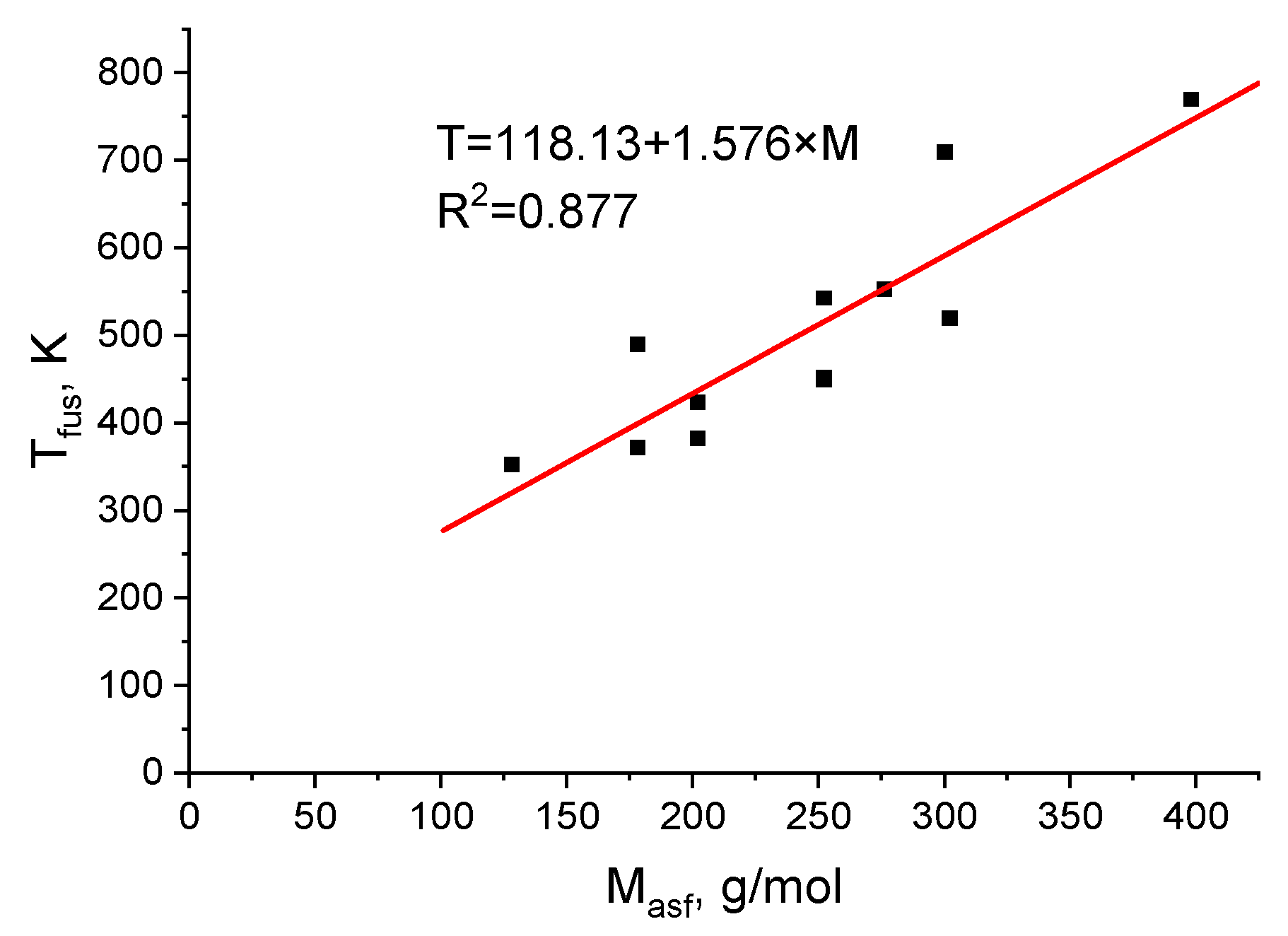
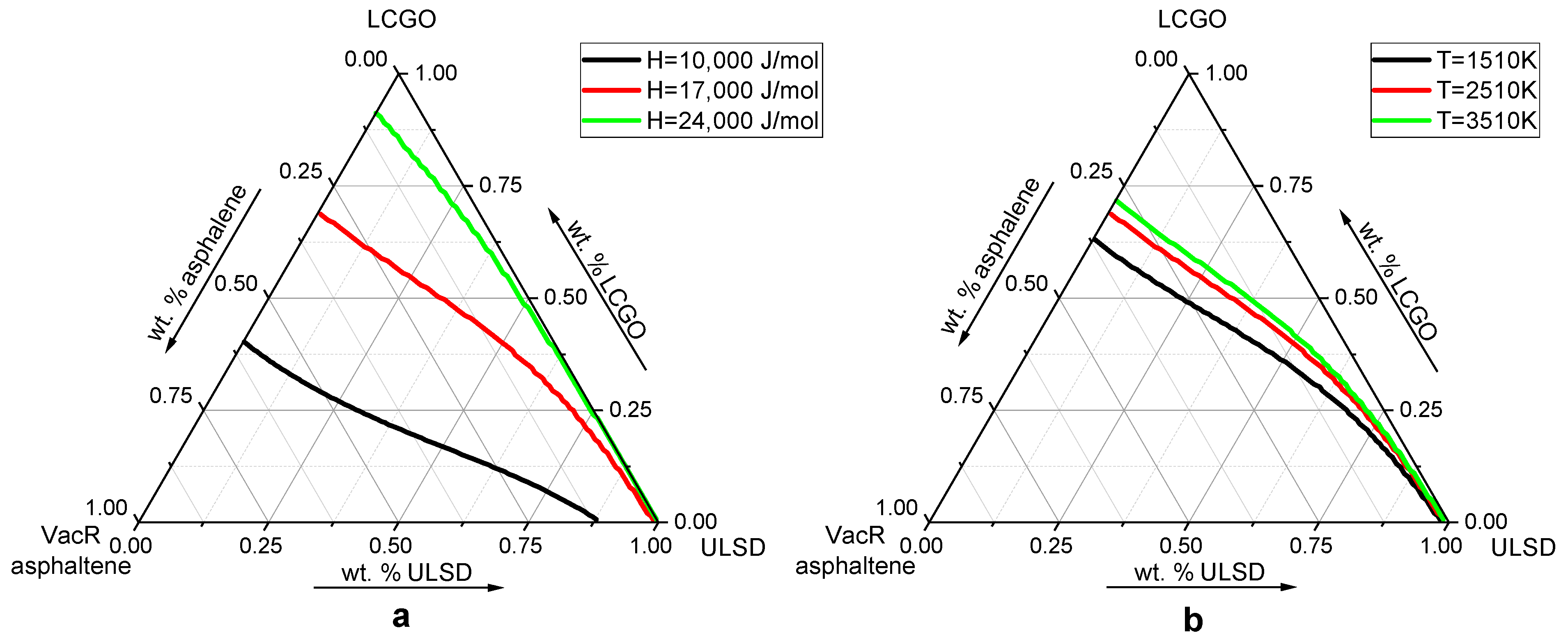
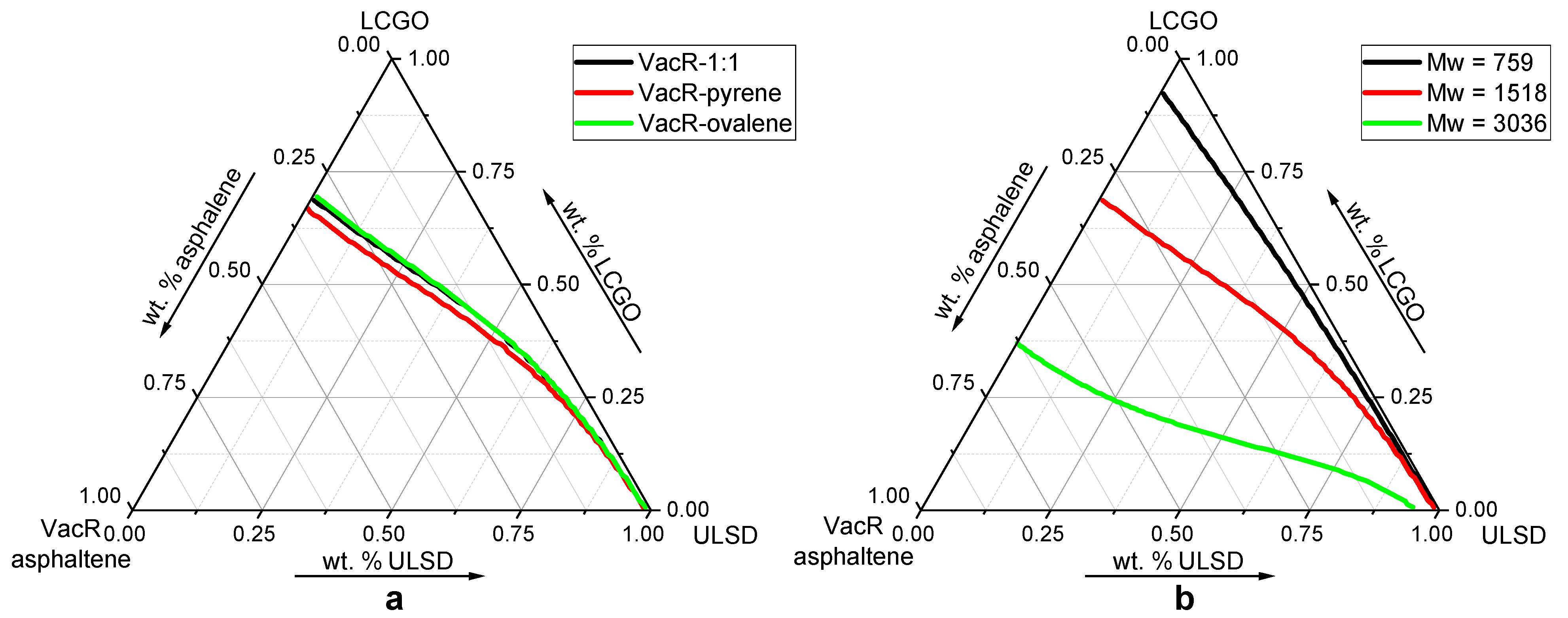
3.3. Influence of the Main Characteristics of Asphaltenes on the Simulation Results

First of all, the sensitivity of the model to the changes in the main parameters (molecular weight, heat and melting temperature of asphaltenes, and their group composition) was tested. These parameters are either averaged (molecular weight and group composition) or obtained by extrapolation (temperature and heat of fusion). Solubility isotherms in the VacR(asphaltene)–ULSD–LCGO system at a heat of fusion of 17 kJ/mol and a melting point of 2510 K were taken as a comparison system.

Figure 2 shows that the heat of fusion of asphaltene has the greatest influence on the position of the isotherm. The smaller it is, the higher the solubility of asphaltene for any composition of the solvent, since the contribution from the heat of fusion to the chemical potential is determined by the value according to Equation (9):

$${\mu }_{add}=RTln{\gamma }_{add}=\frac{\Delta T·\lambda }{T_0}$$

(9)

Here, γ_add is the activity coefficient multiplier showing the effect of the melting process on the chemical potential of asphaltene.

The contribution of RTlnγ_add at an experimental temperature of 400 K, asphaltene melting point of 1500 K, value of ΔT = 1100 K, and heat of fusion of 10,000 J/mol will be 12,500 J/mol. For the quantity γ_add the value equal to 7.4 is obtained. With an increase in the heat of fusion by 1.5 times, the contribution will increase to the power of 3/2 and will be 20.12. On the other hand, the influence of the melting temperature of asphaltene is insignificant which follows from the same formula. Indeed, by increasing T₀ to 2500 K, ΔT is simultaneously increased to 2100 K. The ΔT/T₀ ratio changes from 11/15 to 21/25, so it is increased by only 10%. Thereafter, γ_add will also increase by only 10%.

The effect of variations in the asphaltene structure on the solubility curve also turned out to be insignificant. However, the structure varied in the range of pyrene-ovalene k values. It was considered that the polyaromatic frame of the studied asphaltene is similar to either pyrene or ovalene in terms of the ratio of carbon atoms with hydrogen to carbon atoms without hydrogen (N_ACH/N_AC). For pyrene (C₁₆H₁₀), it is 10/6, and for ovalene (C₃₂H₁₄), it is 14/18. For more complex structures, a more noticeable effect is also possible. The calculation results are shown in Figure 3a.

A specific interest is the effect of asphaltene molecular weight on its solubility. To describe this, the solubility isotherms of asphaltene with an increase in its molecular weight, but while maintaining the ratios between the groups, can be compared. Asphaltene VacR with a molecular weight of 1518 g/mol and the initial group composition presented in Table 2 is taken as an example. If the amount of each group is doubled, a molecular weight will be 3036 g/mol, and if it is reduced by 2 times, then it will be 759 g/mol. Figure 3b shows the corresponding isotherms. A fact that a change in molecular weight is necessarily accompanied by a change in the calculated melting temperature of asphaltene is considered during the calculation. The calculation of the temperature of fusion was carried out according to the correlation equation presented in Figure 1 and amounted to 1307 K for asphaltene with a mass of 759 g/mol and 4903 K for asphaltene with a mass of 3036 g/mol. The curves presented in Figure 3b show that the increase in molecular weight leads to a sharp increase in the solubility of asphaltene. Since the effect of melting temperature in the considered range of ΔT/T₀ is negligible (Figure 2b), the main contribution to the increase in solubility should be attributed to the molecular weight of asphaltene.

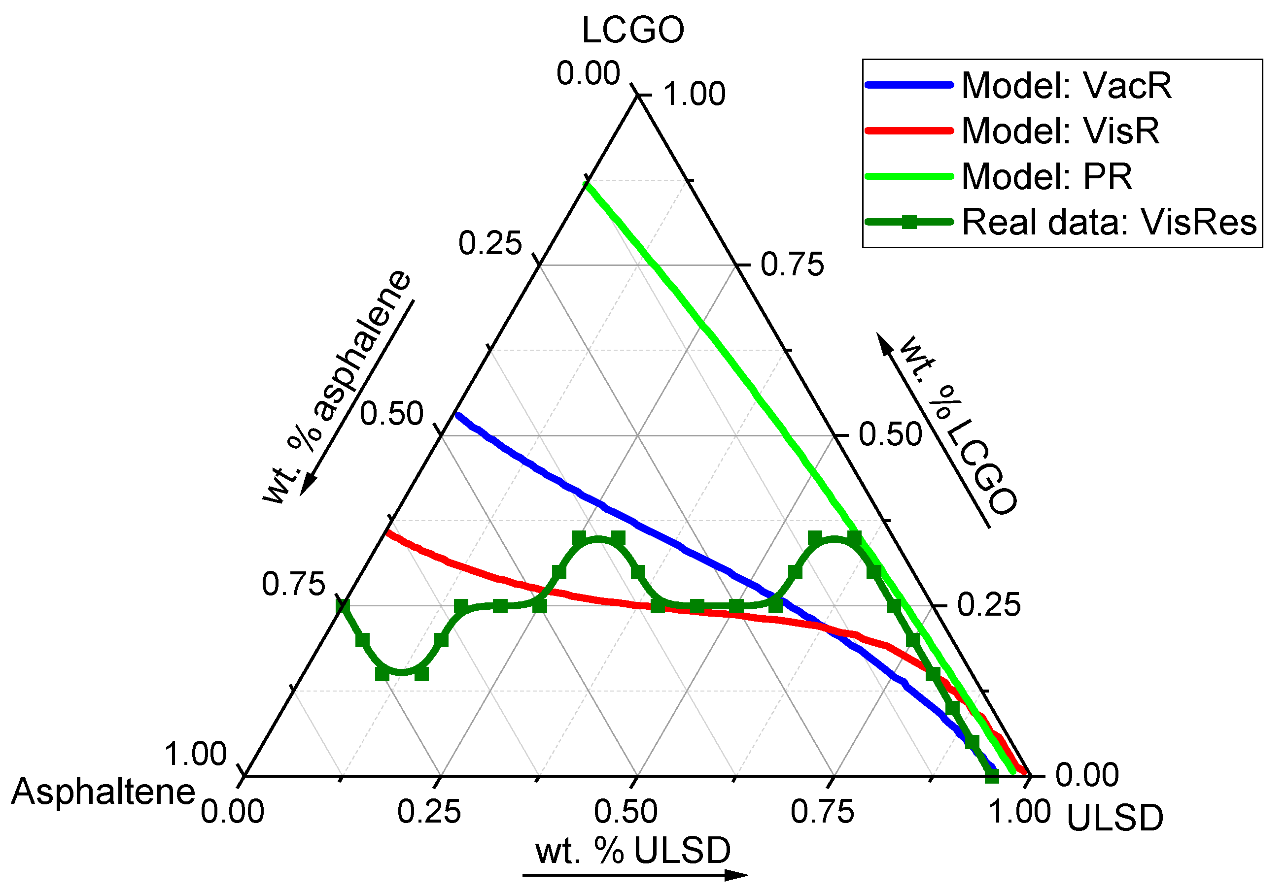
3.4. Comparison of Model Calculations with Experimental Data on the Solubility of Asphaltenes

When comparing the considered model with the experiment the data published in work [54] was used. In this work, the solubility of asphaltene-containing substances in a mixture of two solvents of different polarity was studied at a temperature of 100 °C. The first solvent was hydrotreated diesel cut (ULSD), and the second was light gas oil catalytic cracking (light cycle gas oil) (LCGO). ULSD mainly consists of C₁₂–C₂₀ normal alkanes, while LCGO consists of alkylbenzenes and hydrogenated naphthalenes. The exact composition of both fuels was determined by GCMS method. The group composition used for modeling was established from these data. These data are presented in Section 2.

The low solubility of marine fuels asphaltenes in alkane solvents leads to the sedimentation instability of the system and is characterized by a total sediment after aging (TSA (analysis of “total sediment after chemical aging” ISO 10307-2-2009)) greater than 0.1 wt.% The upper, sedimentation stable area where VisR asphaltenes are soluble in LCGO and ULSD solvents at given ratios, and a lower, sedimentation unstable area where VisR asphaltenes are insoluble in LCGO and ULSD solvents at given ratios, are divided by the curved line.

The three smooth curves shown in Figure 4 show the change in the solubility of each of the asphaltenes shown in Table 2 as a function of the solvent composition. The broken line shows the experimentally obtained solubility limit of VisR (component of marine fuel containing VisR asphaltenes) in the same solvents. It can be seen that the model curve for VisR asphaltenes is located closest to the experimental points.

For samples with a molecular weight of 1518 g/mol the average deviation is also not so large, but due to the absence of an inflection on the theoretical isotherm, the solubility change trend is poorly conveyed. The situation is even worse with the mass of 450 g/mol sample isotherm. In fact, in general, it incorrectly shows the solubility process in the rich in aromatic hydrocarbons area.

This result should be considered in conjunction with the results of the previous section. Two of the four most important characteristics of asphaltenes (heat of fusion, melting point, molecular weight and group composition) viz. the heat of fusion and molecular weight have the greatest influence on solubility. By decreasing the heat of fusion and increasing the molecular weight, a sufficiently large solubility value can be obtained. However, the heat of fusion was taken as an average value for polyaromatic hydrocarbons and was not measured experimentally. On the contrary, the average molecular weight and elemental composition were determined experimentally. The proposed model is supported by the fact that the best agreement between the theoretical isotherm and the experimental data was obtained for the experimental parameters.

The proposed model has similar trends, but differs significantly from the data obtained experimentally, since the experimental curve in the diagram is built using the marine fuel component, visbreaking residue, which contains 26.6 wt.% asphaltenes, not pure asphaltenes. Undoubtedly, the hydrocarbon composition of the fuel (namely, the content of resins and arenes) influences the stability of the fuel system the most. When considering a system consisting of VisR, and not VisR asphaltenes in pure form, and two solvents (ULSD and LCGO) in the same ratios, the dispersed medium will have a different hydrocarbon composition, so when comparing the data obtained, only the trends in the solubility of asphaltenes can be discussed.

To summarize the results obtained, Figure 5 shows the calculation of the solubility of asphaltenes in a hypothetical solution of two groups of the UNIFAC model: AC and CH₂. In this case, they represent a generalization of the aromatic and aliphatic components of petroleum products. In these coordinates, the solubility isotherms are practically straight lines. The solubility of asphaltenes in both groups is less than 10 mass percent. The non-linear course of the solubility isotherm in the case of using ULSD and LCGO as a solvent is explained by the fact that they both contain both aromatic and aliphatic groups. Due to the simultaneous presence of these groups at once in ULSD and LCGO, the isotherm bends, as shown in Figure 4. In addition, the display of solubility in group coordinates can be used as a generalized image, since any oil product can be represented as an average compound with a certain group composition (one of the variants of such a representation was shown earlier). The greatest influence on the solubility of asphaltene when using this method will be exerted by the molecular weight of asphaltene and solvents (petroleum products).

4. Conclusions

The proposed approach to describing the solubility isotherms of asphaltenes in marine fuel is based on the combined use of data on the composition of asphaltenes (from elemental analysis data), their molecular weight and group theories of solutions. At the same time, elemental analysis data is presented in the form of typical groups of the UNIFAC model, which makes it easy to use this data to predict the physicochemical properties, in particular the sedimentation stability of residual marine fuels.

Two of the four main physical and chemical characteristics of asphaltenes (heat of fusion, melting point, molecular weight and group composition) viz. the heat of fusion and molecular weight have the greatest influence on solubility. The weak influence of melting point is due to the fact that the typical melting temperature of asphaltenes (when extrapolated from PAH) is more than 2000 K, due to which the reciprocal value of the melting temperature of asphaltenes (1/T_f) has little effect on the calculation. The weak influence of the group composition is due to the fact that with a change in the k parameter (the ratio of the number of ACH and AC groups in the polyaromatic fragment of the asphaltene molecule), the ratio of the ACH and AC groups (which are one group in terms of intergroup interactions and do not contribute to residual activity factor) mainly changes. In this case, when varying the parameter k, the number of alkyl groups will change insignificantly. Molecular weight primarily affects the solubility isotherm position in a three-component phase diagram, expressed in mass fractions. A possible method of using the proposed approach is to display solubility isotherms in generalized aliphatic–aromatic group coordinates, because any residual marine fuel can be represented as a mixture of aliphatic and aromatic groups.

As a result of comparing the obtained model and experimental data, it was found that they have similar trends. Additionally, they differ significantly from each other due to the fact the experimental three-component phase diagram was built using the marine fuel component, visbreaking residue, which contains 26.6 wt.% asphaltenes, not pure asphaltenes. The development of structure-based solubility prediction models will significantly reduce the number of real experiments for both scientific and industrial purposes. Absolute accuracy is not required from such models, since in any case, experimental verification of the results is necessary.

References

1. Vedachalam, S.; Baquerizo, N.; Dalai, A.K. Review on impacts of low sulfur regulations on marine fuels and compliance options. Fuel 2022, 310, 122243. [Google Scholar] [CrossRef]
2. Zincir, B.; Deniz, C.; Tunér, M. Investigation of environmental, operational and economic performance of methanol partially premixed combustion at slow speed operation of a marine engine. J. Clean. Prod. 2019, 235, 1006–1019. [Google Scholar] [CrossRef]
3. Filatova, I.; Nikolaichuk, L.; Zakaev, D.; Ilin, I. Public-Private partnership as a tool of sustainable development in the oil-refining sector: Russian case. Sustainability 2021, 13, 5153. [Google Scholar] [CrossRef]
4. Khoroshev, V.; Popov, L.; Gatin, R. Prospects of alternative fuels for marine power plants. Trans. Krylov State Res. Cent. 2019, 4, 194–202. [Google Scholar] [CrossRef]
5. Tcvetkov, P. Climate policy imbalance in the energy sector: Time to focus on the value of CO2 utilization. Energies 2021, 14, 411. [Google Scholar] [CrossRef]
6. Litvinenko, V.; Bowbrick, I.; Naumov, I.; Zaitseva, Z. Global guidelines and requirements for professional competencies of natural resource extraction engineers: Implications for ESG principles and sustainable development goals. J. Clean. Prod. 2022, 338, 130530. [Google Scholar] [CrossRef]
7. Mardashov, D.; Duryagin, V.; Islamov, S. Technology for improving the efficiency of fractured reservoir development using gel-forming compositions. Energies 2021, 14, 8254. [Google Scholar] [CrossRef]
8. Vráblík, A.; Velvarská, R.; Štěpánek, K.; Pšenička, M.; Hidalgo, J.M.; Černý, R. Rapid models for predicting the low-temperature behavior of diesel. Chem. Eng. Technol. 2019, 42, 735–743. [Google Scholar] [CrossRef]
9. Sultanbekov, R.; Islamov, S.; Mardashov, D.; Beloglazov, I.; Hemmingsen, T. Research of the influence of marine residual fuel composition on sedimentation due to incompatibility. J. Mar. Sci. Eng. 2021, 9, 1067. [Google Scholar] [CrossRef]
10. Stratiev, D.; Shishkova, I.; Tankov, I.; Pavlova, A. Challenges in characterization of residual oils. A review. J. Pet. Sci. Eng. 2019, 178, 227–250. [Google Scholar] [CrossRef]
11. Vráblík, A.; Schlehöfer, D.; Dlasková Jaklová, K.; Hidalgo Herrador, J.M.; Černý, R. Comparative study of light cycle oil and naphthalene as an adequate additive to improve the stability of marine fuels. ACS Omega 2022, 7, 2127–2136. [Google Scholar] [CrossRef] [PubMed]
12. Gaile, A.A.; Vereshchagin, A.V.; Klement’ev, V.N. Refining of diesel and ship fuels by extraction and combined methods. Part 1. Use of ionic liquids as extractants. Russ. J. Appl. Chem. 2019, 92, 453–475. [Google Scholar] [CrossRef]
13. Gaile, A.A.; Vereshchagin, A.V.; Klement’ev, V.N. Refining of diesel and ship fuels by extraction and combined methods. Part 2. Use of organic solvents as extractants. Russ. J. Appl. Chem. 2019, 92, 583–595. [Google Scholar] [CrossRef]
14. Sultanbekov, R.; Beloglazov, I.; Islamov, S.; Ong, M. Exploring of the incompatibility of marine residual fuel: A case study using machine learning methods. Energies 2021, 14, 8422. [Google Scholar] [CrossRef]
15. Yakubov, M.R.; Abilova, G.R.; Yakubova, S.G.; Milordov, D.V.; Mironov, N.A. 4 Heavy oil resin composition and their influence on asphaltene stability. In The Chemistry of Oil and Petroleum Products; De Gruyter: Berlin, Germany, 2022; pp. 177–202. [Google Scholar]
16. Vasilyev, V.V.; Salamatova, E.V.; Maidanova, N.V.; Kalinin, M.V.; Strakhov, V.M. Change in properties of roadmaking bitumen on oxidation. Coke Chem. 2020, 63, 307–314. [Google Scholar] [CrossRef]
17. Wang, L.-T.; Hu, Y.-Y.; Wang, L.-H.; Zhu, Y.-K.; Zhang, H.-J.; Huang, Z.-B.; Yuan, P.-Q. Visbreaking of heavy oil with high metal and asphaltene content. J. Anal. Appl. Pyrolysis 2021, 159, 105336. [Google Scholar] [CrossRef]
18. Mardashov, D.; Bondarenko, A.; Raupov, I. Technique for calculating technological parameters of non-Newtonian liquids injection into oil well during workover. J. Min. Inst. 2022. Online first. [Google Scholar] [CrossRef]
19. Didmanidze, O.; Afanasev, A.; Khakimov, R. Mathematical model of the liquefied methane phase transition in the cryogenic tank of a vehicle. J. Min. Inst. 2020, 243, 337. [Google Scholar] [CrossRef]
20. Sultanbekov, R.R.; Shammazov, I.A.; Schipachev, A.M. Determination of compatibility and stability of residual fuels before mixing in tanks. Pet. Eng. 2021, 19, 128. [Google Scholar] [CrossRef]
21. Nguele, R.; Mbouopda Poupi, A.B.; Anombogo, G.A.M.; Alade, O.S.; Saibi, H. Influence of asphaltene structural parameters on solubility. Fuel 2022, 311, 122559. [Google Scholar] [CrossRef]
22. Nazarenko, M.Y.; Kondrasheva, N.K.; Saltykova, S.N. The effect of thermal transformations in oil shale on their properties. Tsvetnye Met. 2017, 29–33. [Google Scholar] [CrossRef]
23. Raupov, I.; Burkhanov, R.; Lutfullin, A.; Maksyutin, A.; Lebedev, A.; Safiullina, E. Experience in the application of hydrocarbon optical studies in oil field development. Energies 2022, 15, 3626. [Google Scholar] [CrossRef]
24. Kass, M.D.; Armstrong, B.L.; Kaul, B.C.; Connatser, R.M.; Lewis, S.; Keiser, J.R.; Jun, J.; Warrington, G.; Sulejmanovic, D. Stability, combustion, and compatibility of high-viscosity heavy fuel oil blends with a fast pyrolysis bio-oil. Energy Fuels 2020, 34, 8403–8413. [Google Scholar] [CrossRef]
25. Álvarez, E.; Trejo, F.; Marroquín, G.; Ancheyta, J. The effect of solvent washing on asphaltenes and their characterization. Pet. Sci. Technol. 2015, 33, 265–271. [Google Scholar] [CrossRef]
26. Guzmán, R.; Ancheyta, J.; Trejo, F.; Rodríguez, S. Methods for determining asphaltene stability in crude oils. Fuel 2017, 188, 530–543. [Google Scholar] [CrossRef]
27. Hosseini-Dastgerdi, Z.; Tabatabaei-Nejad, S.A.R.; Khodapanah, E.; Sahrae, E. A comprehensive study on mechanism of formation and techniques to diagnose asphaltene structure; molecular and aggregates: A review. Asia-Pac. J. Chem. Eng. 2014, 10, 743–753. [Google Scholar] [CrossRef]
28. Zhang, Y.; Siskin, M.; Gray, M.R.; Walters, C.C.; Rodgers, R.P. Mechanisms of asphaltene aggregation: Puzzles and a new hypothesis. Energy Fuels 2020, 34, 9094–9107. [Google Scholar] [CrossRef]
29. Vatti, A.K.; Caratsch, A.; Sarkar, S.; Kundarapu, L.K.; Gadag, S.; Nayak, U.Y.; Dey, P. Asphaltene aggregation in aqueous solution using different water models: A classical molecular dynamics study. ACS Omega 2020, 5, 16530–16536. [Google Scholar] [CrossRef]
30. Lebedev, A.B.; Musinova, P.V. Formation of the strength of pelletized multiphase dicalcium silicate sinter. Chernye Metally 2022, 2022, 40–46. [Google Scholar] [CrossRef]
31. Li, H.; Zhang, Y.; Xu, C.; Zhao, S.; Chung, K.H.; Shi, Q. Quantitative molecular composition of heavy petroleum fractions: A case study of fluid catalytic cracking decant oil. Energy Fuels 2020, 34, 5307–5316. [Google Scholar] [CrossRef]
32. Jiguang, L.; Xin, G.; Haiping, S.; Xinheng, C.; Ming, D.; Huandi, H. The solubility of asphaltene in organic solvents and its relation to the molecular structure. J. Mol. Liq. 2021, 327, 114826. [Google Scholar] [CrossRef]
33. Litvinova, T.; Kashurin, R.; Zhadovskiy, I.; Gerasev, S. The kinetic aspects of the dissolution of slightly soluble lanthanoid carbonates. Metals 2021, 11, 1793. [Google Scholar] [CrossRef]
34. Ershov, M.A.; Savelenko, V.D.; Shvedova, N.S.; Kapustin, V.M.; Abdellatief, T.M.M.; Karpov, N.V.; Dutlov, E.V.; Borisanov, D.V. An evolving research agenda of merit function calculations for new gasoline compositions. Fuel 2022, 322, 124209. [Google Scholar] [CrossRef]
35. Ershov, M.A.; Savelenko, V.D.; Makhova, U.A.; Kapustin, V.M.; Abdellatief, T.M.M.; Karpov, N.V.; Dutlov, E.V.; Borisanov, D.V. Perspective towards a gasoline-property-first approach exhibiting octane hyperboosting based on isoolefinic hydrocarbons. Fuel 2022, 321, 124016. [Google Scholar] [CrossRef]
36. Litvinenko, V.; Tsvetkov, P.; Dvoynikov, M.; Buslaev, G. Barriers to implementation of hydrogen initiatives in the context of global energy sustainable development. J. Min. Inst. 2020, 244, 421. [Google Scholar] [CrossRef]
37. Mohammed, I.; Mahmoud, M.; Al Shehri, D.; El-Husseiny, A.; Alade, O. Asphaltene precipitation and deposition: A critical review. J. Pet. Sci. Eng. 2021, 197, 107956. [Google Scholar] [CrossRef]
38. Painter, P.; Veytsman, B.; Youtcheff, J. Guide to asphaltene solubility. Energy Fuels 2015, 29, 2951–2961. [Google Scholar] [CrossRef]
39. Andersen, S.I.; Speight, J.G. Thermodynamic models for asphaltene solubility and precipitation. J. Pet. Sci. Eng. 1999, 22, 53–66. [Google Scholar] [CrossRef]
40. Gracin, S.; Brinck, T.; Rasmuson, Å.C. Prediction of solubility of solid organic compounds in solvents by UNIFAC. Ind. Eng. Chem. Res. 2002, 41, 5114–5124. [Google Scholar] [CrossRef]
41. Kuramochi, H.; Maeda, K.; Kato, S.; Osako, M.; Nakamura, K.; Sakai, S. Application of UNIFAC models for prediction of vapor-liquid and liquid-liquid equilibria relevant to separation and purification processes of crude biodiesel fuel. Fuel 2009, 88, 1472–1477. [Google Scholar] [CrossRef]
42. Parameters of the Original UNIFAC Model. Available online: http://www.ddbst.com/PublishedParametersUNIFACDO.html (accessed on 30 May 2022).
43. Pytherm. Calculation Programm. Available online: https://github.com/PsiXYZ/pytherm (accessed on 15 September 2021).
44. IUPAC-NIST Solubility Database, Version 1.1. Available online: https://srdata.nist.gov/solubility/ (accessed on 30 May 2022).
45. Smutek, M.; Friš, M.; Frohl, J. Kristallisationsgleichgewichte V. Löslichkeiten des anthrazens und carbazols in einigen misch-lösungsmitteln. Collect. Czechoslov. Chem. Commun. 1967, 32, 931–943. [Google Scholar] [CrossRef]
46. Choi, P.B.; Mclaughlin, E. Effect of a phase transition on the solubility of a solid. AIChE J. 1983, 29, 150–153. [Google Scholar] [CrossRef]
47. Acree, W.E.; Rytting, J.H. Solubility in binary solvent systems III: Predictive expressions based on molecular surface areas. J. Pharm. Sci. 1983, 72, 292–296. [Google Scholar] [CrossRef] [PubMed] [Green Version]
48. Chang, W. Solubilities of Biphenyl, Naphthalene, Perfluorobiphenyl, Perfluoronaphthalene and Hexachloroethane in Nonelectrolytes; North Dakota State University: Fargo, ND, USA, 1969. [Google Scholar]
49. Choi, P.B.; Williams, C.P.; Buehring, K.G.; McLaughlin, E. Solubility of aromatic hydrocarbon solids in mixtures of benzene and cyclohexane. J. Chem. Eng. Data 1985, 30, 403–409. [Google Scholar] [CrossRef]
50. Pyagai, I.; Zubkova, O.; Babykin, R.; Toropchina, M.; Fediuk, R. Influence of impurities on the process of obtaining calcium carbonate during the processing of phosphogypsum. Materials 2022, 15, 4335. [Google Scholar] [CrossRef]
51. Lyakh, D.D.; Khudyakova, I.N.; Ivanov, S.L. Justification of peat block-making module parameters and mass/power characteristics for peat production machinery. Min. Inform. Anal. Bull. 2022, 6, 93–108. [Google Scholar] [CrossRef]
52. Pyagay, I.N.; Shaidulina, A.A.; Konoplin, R.R.; Artyushevskiy, D.I.; Gorshneva, E.A.; Sutyaginsky, M.A. Production of amorphous silicon dioxide derived from aluminum fluoride industrial waste and consideration of the possibility of its use as Al2O3-SiO2 catalyst supports. Catalysts 2022, 12, 162. [Google Scholar] [CrossRef]
53. Zubkova, O.; Alexeev, A.; Polyanskiy, A.; Karapetyan, K.; Kononchuk, O.; Reinmöller, M. Complex processing of saponite waste from a diamond-mining enterprise. Appl. Sci. 2021, 11, 6615. [Google Scholar] [CrossRef]
54. Kondrasheva, N.K.; Rudko, V.A.; Kondrashev, D.O.; Shakleina, V.S.; Smyshlyaeva, K.I.; Konoplin, R.R.; Shaidulina, A.A.; Ivkin, A.S.; Derkunskii, I.O.; Dubovikov, O.A. Application of a ternary phase diagram to describe the stability of residual marine fuel. Energy Fuels 2019, 33, 4671–4675. [Google Scholar] [CrossRef]
Figure 1. Correlation dependence of the melting point of polyaromatic compounds on their molecular weight.
Jmse 10 01017 g001
Figure 2. Asphaltene solubility at various parameters (composition is indicated in mass fractions): (a) melting heats; (b) melting temperatures. Hereinafter, the asphaltene solubility isotherm VacR at 298 K and other characteristics presented in Table 2 are taken as a comparison system.
Jmse 10 01017 g002
Figure 3. Three-component phase diagrams (the composition is indicated in mass fractions): (a) the effect of the group composition of asphaltene on its solubility; (b) influence of asphaltene molecular weight on the solubility isotherm.
Jmse 10 01017 g003
Figure 4. Simulation results of the asphaltene–ULSD–LCGO system in comparison with the data obtained experimentally (the composition is indicated in mass fractions).
Jmse 10 01017 g004
Figure 5. The results of calculating the solubility of the studied asphaltenes in a hypothetical solution of aromatic (AC) and aliphatic (CH2) groups at a temperature of 373 K (the composition is indicated in mass fractions).
Jmse 10 01017 g005