Article

Water Circulation and Transport Time Scales in the Beagle Channel, Southernmost Tip of South America

by
Andrea Cucco
1,*,
Jacobo Martín
2,3,
Giovanni Quattrocchi
1,
Harold Fenco
4,
Georg Umgiesser
5,6 and
Daniel Alfredo Fernández
7,8
1
Institute for the Study of Anthropic Impacts and Sustainability in the Marine Environment, CNR-IAS, 09170 Oristano, Italy
2
Laboratorio de Oceanografía, CADIC-CONICET, Houssay 200, Ushuaia CP 9410, Argentina
3
Departament de Dinàmica de la Terra i de l’Oceà, Universitat de Barcelona (UB), E-08028 Barcelona, Spain
4
Gabinete de Oceanografía Física, INIDEP, Mar del Plata CP 7600, Argentina
5
Institute of Marine Sciences, CNR-ISMAR, 30122 Venice, Italy
6
Marine Research Institute, Klaipeda University, LT-92294 Klaipeda, Lithuania
7
Instituto de Ciencias Polares, Ambiente y Recursos Naturales, Universidad Nacional de Tierra del Fuego (ICPA-UNTDF), Ushuaia CP 9410, Argentina
8
Laboratorio de Ecología, Fisiología y Evolución de Organismos Acuáticos, CADIC-CONICET, Houssay 200, Ushuaia CP 9410, Argentina
*
Author to whom correspondence should be addressed.
J. Mar. Sci. Eng. 2022, 10(7), 941; https://doi.org/10.3390/jmse10070941
Submission received: 7 June 2022 / Revised: 1 July 2022 / Accepted: 5 July 2022 / Published: 8 July 2022
(This article belongs to the Special Issue Dynamics in Coastal Areas)

Abstract

:
The Beagle Channel is a long and narrow interoceanic passage within the Tierra del Fuego archipelago in the southernmost tip of South America. A high-resolution 3D hydrodynamic model based on the finite elements method was applied to investigate the residual circulation, water fluxes and transport time scales inside this channel. Numerical solutions were analyzed at seasonal time scale and the model results compared with observed ocean data. The circulation pattern is characterized by a west-to-east residual flow with low intensity and low seasonal variability. The water fluxes through the channel were estimated to be, on average, around 12,700 m3/s, with inflow through its western entrance and eastwards outflow mainly through the Mackinlay Strait. The water residence times vary seasonally with basin averages between 36 and 43 days and maximum values between 53 and 95 days. The results provide an overview of the hydrodynamics and water residence times in the Beagle Channel, a unique ecosystem threatened by recent anthropogenic pressures and climate change.

1. Introduction

The Beagle Channel (hereafter BC) is a 270 km-long interoceanic passage situated at the southernmost point of South America, connecting the Pacific and the Atlantic oceans at latitude 55° S (see Figure 1A).
The channel is characterized by the presence of multiple shoals, islands and relatively confined sub-basins. From the Pacific Ocean eastwards, the Southwest and Northwest branches converge at Punta Divide, forming the central Beagle Channel that progresses to the east until opening towards the Atlantic Ocean, south of the Mitre Peninsula (see Figure 1B,C). Both western branches present sharp bathymetric constraints as shallow as 20–60 m [1] separating basins several hundred meters deep, a condition that hampers the free flow of sub-surface Subantarctic Waters [2]. Towards the east, another two shallow passages at the Murray Channel and Mackinlay Strait impose abrupt bathymetric blockages to the water flow.
The southern end of South America is part of the Patagonian cold estuarine zone [3]. The prevailing westerlies transport great amounts of humidity that produce heavy rain by orographic control upon encountering the Andean Mountain range.
Two surface branches of the South Pacific Current diverge upon encountering the Chilean Patagonia, one flowing to the north (Humboldt Current, out of the investigated domain) and a second one, the Cape Horn Current (CHC, see Figure 1A) that flows poleward and contours anticyclonically the tip of the subcontinent. The CHC transports low-salinity waters from the Southeast Pacific, whose influence extends to the Atlantic Patagonian Shelf [4].
A dense network of rivers and streams open to the BC, mainly along its central and eastern courses. Freshwater inputs from snow and glacier melting are deemed to be more relevant in the western sector, on the Pacific side of the Northwest branch, where Cordillera Darwin (see Figure 1B) holds one of the largest ice fields in the Southern Hemisphere [5]. Thermal and hydrological cycles are characterized by seasonality with maximum air temperature and water discharges in the austral summer and minima in winter. Even though total precipitation is important in winter, these are retained on land as ice and snow, and released during the summer freshet [6].
The Beagle Channel presents a microtidal regime (typical amplitudes 0.5 to 1 m; [7]). A net eastward surface flow has been observed [8,9] while a counter-clockwise circulation cell has been described at Ushuaia Bay [8,10,11].
The current knowledge about the water circulation and flushing features of the channel is, at present, very limited. Up to now, in fact, only a few studies have been published mainly to describe the time and space variability of water temperature and salinity [12] or to investigate the wind- and tide-induced water circulation in confined traits of the BC [10,11]. Advancing in our understanding of the general circulation and water residence times of the BC is, nowadays, a pressing matter in relation to climate change and anthropogenic threats.
Although most of the channel remains unpopulated, there has been continued growth in intense maritime traffic and human settlements in recent decades. In particular, the port and city of Ushuaia (about 80,000 inhabitants) has become a significant pressure on local ecosystems and a source of pollutants to the channel [13,14,15]. The dispersion routes and final fate of pollutants, including wastewaters and eventual oil spills, are not satisfactorily understood at present.
Within this context, the evaluation of the local transport time scales is crucial to estimate the channel renewal features. In particular, water residence times influence the water quality and the ecological status of marine coastal systems by controlling the physical, chemical, and biological processes taking place there [16,17,18,19]. They play a significant role in shaping the spatio-temporal distribution of pollutants and nutrients in coastal water bodies, thus influencing both the gross primary production, the trophic web structure and the eutrophication of coastal aquatic environments [20,21].
In recent decades, the increase in anthropogenic nutrient fluxes in the BC has increased the risk of dystrophic events, especially in confined and urbanized areas such as the Ushuaia Bay [15], where local cleaning capacity and the upper limits for a sustainable level of the nutrients loads need to be established.
Furthermore, the runoff of organic matter and nutrients loads produced from the vast forests surrounding the BC, influences the marine trophic web and ecosystem assemblage inside the channel [22,23]. Along with the seasonal variability of mainland fluxes, the water circulation and the flushing features play an important role in shaping the final distribution of nutrients and organic matter in the BC.
The water residence times are also key factors in determining the rate at which eggs and larvae of marine species are exchanged with the open ocean [24,25,26]. In this regard, the BC is a nursery area for different fish species [27] and the knowledge of those zones characterized by hydrodynamic conditions promoting the retention of larvae and eggs is a fundamental aspect to take into account for a sustainable management of the marine resources.
In addition, the possible future implementation of the fish farming industry in the BC reinforces the need to urgently set baselines of water fluxes and residence times in this unique ecosystem.
Furthermore, in the context of climatic changes, warming temperatures and glacial retreat, the knowledge of the fresh water residence times inside the channel can provide a tool useful to predict the consequences in the local ecosystem assemblages.
For all these reasons, the main goal of this research is to assess the hydrodynamics and the flushing features of the BC, to support a sustainable management of the marine resources of this unique ecosystem.
With this purpose, a high-resolution three-dimensional hydrodynamic model was implemented to reproduce the main circulation of the BC and to estimate the water residence times. The model was applied to the entire channel and results compared with both tidal elevations and water current observations. Seasonal variation of water fluxes, residual flows and water residence times along the channel were analyzed and discussed.
The paper is organized as follows: a detailed description of the adopted numerical method and available oceanographic data in the area is reported in Section 2. In Section 3, the model validation procedure is described, the simulation results are compared with observations and the channel water circulation and transport time scales are analyzed. Finally, in Section 4 the obtained results are discussed and some concluding remarks are put forward.

2. Materials and Methods

2.1. Model Description and Simulation Setup

The water circulation and the transport time scales in the BC have been investigated following a numerical approach. A high-resolution 3D hydrodynamic model (hereafter SHYFEM, [28]), based on the finite element method was applied to reproduce the main hydrodynamics inside the channel and in the surrounding coastal areas.
SHYFEM resolves the three-dimensional primitive equations, resolving the barotropic, baroclinic and atmospheric pressure gradients, wind drag and bottom friction, nonlinear advection, vertical turbulent processes and tidal potential. The model is an open-source code project, freely available at https://github.com/SHYFEM-model (accessed on 1 March 2020), that has been applied with success to simulate the hydrodynamics in both open seas and coastal waters, e.g., [29,30,31,32,33], and to compute the transport time scales of lagoons and semi-enclosed basins (see [34] and references therein). The model uses the finite element method for the horizontal spatial discretization of the state variables, z-layers for the vertical discretization and a semi-implicit algorithm for the temporal integration. This method has the advantage of being unconditionally stable with respect to gravity waves, bottom friction and Coriolis terms allowing the transport of the variables to be solved explicitly.
The hydrodynamic model is coupled with a three-dimensional transport and diffusion numerical module that take into account the salt and thermal balance equations to simulate the transport of both passive tracers, salinity and temperature in the domain. In Appendix A, a detailed description of the hydrodynamic and transport equations systems solved by the model is reported.
The numerical application was carried out on a domain extending approximately between 87° W, 70° S and 50° W, 37° S and comprises the entire BC, part of the Drake Passage (see Figure 2), Southeast Pacific and Southwest Atlantic. The numerical computation is carried out on an unstructured mesh composed of 71,954 nodes and 132,426 triangular elements with a spatial resolution varying between 50 m for the inner part of the BC and 50 km for the far field.
In Figure 2A–C, magnifications of the model mesh for the BC area are depicted. The mesh represents the whole channel extending from its western branches (Noroeste and Suroeste channels, see Figure 1C), to the eastern opening, with higher geometric detail in the central BC section where the highest density of computational nodes was defined. The use of elements of variable sizes is fully exploited, in order to suit the geometry of the channel characterized by a sinuous coastline, islands and sharp bathymetric changes.
The morphology of the computational domain was reconstructed merging different set of bathymetric sources including the GEBCO dataset [35], available at 1 min and 30 s arc spatial resolution, for the outer ocean regions and data obtained from the digitalization of nautical charts (SHOA, Chilean Hydrographic Service charts 22430 and 22418; Argentinian Hydrographic Service chart H-477) for the Tierra del Fuego Archipelagos and BC regions. In Figure 2D, the bathymetric details of the central part of the BC, extending from Punta Divide, on the west, to the eastern mouth of the channel next to Picton Island, are reported as reproduced by the finite element mesh.
The vertical direction was discretized by 27 uneven z-levels with layer thicknesses varying from 5 m, for the uppermost layer, to 3000 m for the ocean seafloor and following an ad hoc step distribution with the first 100 m of water depth discretized by 9 layers.
The surface and bottom friction terms were computed following a quadratic law (see Equation (A2) in Appendix A) with the wind or surface drag coefficient computed according to the Smith and Banke formulation [36] and the bottom drag coefficient Cd set as constant and homogeneous over the whole model domain to the value of 3.1 × 10⁻³. This value was obtained after a model calibration process was performed (see Section 3.1). The water temperature and salinity were computed accounting for surface fluxes, advection and diffusion processes (see Appendix A).
Oceanographic and atmospheric data obtained from different sources were used as model forcing and boundary conditions. Specifically, ocean data were provided by the European Earth Observation Programme Copernicus (https://www.copernicus.eu/en, accessed on 1 May 2020) and included the daily means of temperature, salinity and sea level with horizontal resolution of 1/12 degree and 50 vertical levels, ranging from 0 to 5500 m. These data were produced by the Operational Mercator global ocean analysis and forecast system, based on the ocean model NEMO [37].
The atmospheric data necessary to compute the heat flux and momentum transfer were provided by ERA-Interim [38], a global atmospheric reanalysis performed by the European Centre for Medium-Range Weather Forecasts (ECMWF, https://www.ecmwf.int/node/8174, accessed on 1 May 2020). These data included the air temperature, precipitation, evaporation rate, humidity, atmospheric pressure and wind components with a temporal and spatial resolution of 6 h and approximately 80 km.
Tidal forcing was obtained from the satellite-altimetry-constrained tidal model TPXO7.2 based on updated bathymetry and assimilation procedure [39,40]. TPXO data along the SHYFEM open boundaries were extracted using OTIS (OSU Tidal Inversion Software), a tidal data inversion package described by [39] and further by [40]. In particular, the tidal elevations were reconstructed as complex amplitudes of earth-relative sea-surface elevation for eight primaries (M2, S2, N2, K2, K1, O1, P1, Q1), two long-period (Mf, Mm) and three non-linear (M4, MS4, MN4) harmonic constituents (plus 2N2 and S1 for TPXO9).
Water level boundary conditions were obtained by summing the barotropic contribution constituted by the astronomical tides to the total water elevation obtained from the daily water levels provided by the Copernicus Platform. A Dirichlet boundary condition was adopted, with water levels imposed and current velocities freely computed by the model along the open boundaries. Temperature and salinity fields were nested into the model domain using a nudging procedure following the method proposed by [30] and subsequently adopted by [33]. In particular, temperature and salinity data were interpolated for all nodes and layers of the unstructured mesh to obtain a proper nudging dataset. The value of the relaxation coefficient was set as spatially varying over the model domain from 1 day in the open sea and increasing toward high resolution areas inside the Channel. The nudging allows the model state to cohere with the assimilated Copernicus data in the open sea, thus limiting the error growth, and to fully compute the hydrodynamics in the coastal areas and in the Beagle Channel. At the open boundaries, a radiative condition was used for the temperature and salinity.
Yearly averaged fluxes of the main rivers discharging in the northern (i.e., Argentinian) side of the central BC were obtained from [41] and consisted of 31 freshwater outflows approximately located between the sections S4 and S9 of Figure 2D. The average fluxes were generally low, with most of the values lower than 1 m3/s and highest inflow estimated around 20 m3/s for the Lapataia River located on the western sector and around 11 m3/s for Lasifashaj River on the eastern part of the central BC.
Atmospheric, tidal and ocean data for the years 2015 and 2016 were used as forcing for a 2-year-long numerical run, and only the results for 2016 were analyzed, permitting the noises generated by the model initial conditions to be dumped out. This long spin-up time was adopted due both to the large extension of the model domain and to the use of multiple types of oceanic and atmospheric forcing and boundary conditions.

2.2. Transport Time Scales

Flushing features of semi-enclosed basins as coastal bays, gulfs or lagoons can be defined in many different ways depending on the adopted methods [42,43,44,45,46,47]. In this work, assuming the advection and diffusion as the main physical processes influencing the cleaning capacity of the channel, two main parameters, the turnover time and the water residence times were used to compute the flushing features of the central part of the BC. Both transport time scales were estimated at seasonal frequency and considering only the sector of the BC extending between the sections S3 and S9ab of Figure 2D, as the reference domain.
The turnover time (WTO) is theoretically defined as the time necessary to replace the water volume of a domain with new water. In the present case, the central part of the BC is considered as the domain, with new water entering from the Northwest and Southwest branches and water flowing out of at the eastern limit of the channel. Assuming a fully mixed hydrodynamic condition, considering Q the water flux flowing out of the system and V the volume of the domain, the WTO is defined as [43]:
W T O = V Q
with Q computed from the simulation results as the seasonal and yearly averaged water fluxes across sections S3, S9ab and S6 and V the water volumes contained between S3 and S9ab. River runoff was very low and therefore not influencing the computation of the channel net outflow.
The water residence times or Eulerian transport time scale (WRT) were computed by simulating the transport and diffusion of a conservative tracer released uniformly and with a unitary concentration in the selected domain corresponding to the central BC between sections S3 and S9ab. During the simulation run, the initial unitary tracer concentration was reduced by the mass exchanges between the selected sector and the external domain, where the concentration was set to zero. The WRT was then defined as the time required for each node of the selected domain to replace the mass of the conservative tracer, initially released, with new water. The WRT were locally computed by integrating in time the remnant function of the tracer concentration for the entire duration of the simulation obtaining the e-folding time of the tracer concentration [42]. This method has been widely used to compute and investigate the flushing features of coastal bays, gulfs and lagoons (see [34] and references herein).
The WTO and WRT are based on different methods and provide different information, with WTO quantifying the overall basin flushing time and with WRT providing also information on its spatial variability. The two transport time scales behave differently in relation to the geometry and the hydrodynamics of the basin, and their comparison can be helpful in classifying different water bodies. We refer to [34,48,49] for a detailed description of the computed transport time scales.

2.3. Observations

A set of field data was used to verify the model results and to estimate the model accuracy in reproducing the tidal dynamics and the water circulation in the central BC.
In [50], an accurate study of the tidal propagation in the Tierra del Fuego shelf was carried out, and the harmonics of the main astronomical components were computed for more than 40 locations along the Atlantic Argentinian coasts and in the BC. These data were used to estimate the accuracy of the model in reproducing the tidal propagation in the study area. The comparison between simulation results and experimental data was made for a subset of 23 tidal stations located in the BC and in the coast of Tierra del Fuego up to the Magellan Strait in the north (see Figure 3A).
During December 2016, an oceanographic cruise was carried out in the BC to collect vertical profiles of current speed and direction for several stations along the channel and at its eastern mouth (see Figure 3B) by means of a TRDI WHS 300 kHz Acoustic Doppler Current Profiler, installed in a CTD-Rosette probe. The ADCP was configured to operate in vertical Lowered (LADCP) mode, which provided full-water column profiles of current speed and direction with 4 m vertical resolution cell size. The LADCP data was processed with the LDEO_IX version 10 implementation of the velocity inverse method [51]. The accuracy of the LADCP data was determined to be 5 cm/s [52], and current speed data below that threshold were neglected.
In addition, from 27 May to 1 December 2017, near-bottom time-series of velocity speed and direction was obtained by means of an electromagnetic single-point current meter Infinity AEM (JFE Advantech) in Ushuaia Bay at 68.22° W, 54.82° S (see Figure 3B). The current meter was attached to a mooring line 10 m above bottom (total water depth 130 m depth), and programmed with a sampling rate of 10 min. Accuracy for this current meter data is ±1 cm/s according to the manufacturer.
These datasets were used to validate the model results through direct comparison between LADCP data and modeled current velocities along the BC and by comparing the scatter distributions of the observed and modeled velocity components for the moored current-meter in Ushuaia Bay.

3. Results

3.1. Model Validation

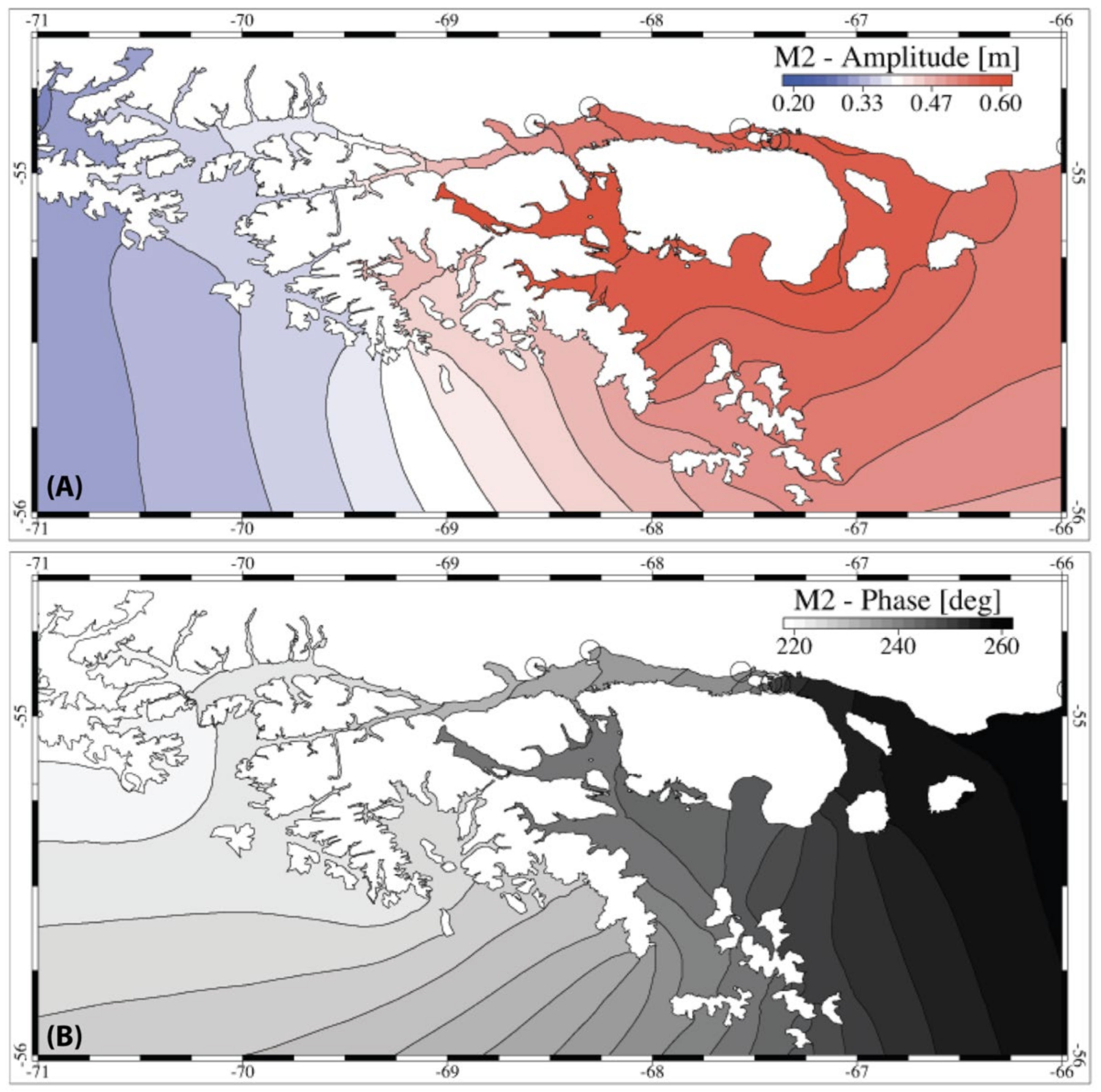
3.1.1. Tidal Elevation

A set of calibration runs was performed comparing the modeled amplitude and phase of the five main tidal constituents, M2, S2, N2, O1 and K1, with observed data. A trial and error method was used considering the bottom friction coefficient Cd (see Equation (A2) in Appendix A), as the model parameter to be changed during the calibration procedure.
The time series of the water levels obtained from the simulation run were processed with the tidal analysis package [53] to compute, for each tidal station, the amplitudes and phases of the M2, S2, N2, O1 and K1 astronomic constituents. The model performance levels were then assessed by calculating, for each tidal station, the vectorial differences d between the observed and the modeled harmonic constants. The metric for estimating the model error reads as:
d i , j = a i , j o cos g i , j o a i , j m cos g i , j m 2 + a i , j o sin g i , j o a i , j m sin g i , j m 2
with a and g the amplitude, expressed in meters, and phase, expressed in degrees, of the tidal harmonics. The subscripts i and j refer to the tidal gauge station and to the tidal constituent, superscript o refers to the observed data and superscript m refers to the model results [54,55]. Finally, for each tidal constituent j, considering the whole set of 23 stations (N), the root mean square deviation of amplitude (RMS) between modeled and observed data was defined following [56] as:
R M S j = 1 2 N i = 1 N d i , j 2
The observed amplitudes and phases (ao and go) and the calibrated model results (am and gm) used as input data in Equation (2) are reported in Table S1 of Supplementary Materials for the whole set of 23 tidal stations and for the 3 semidiurnal and 2 diurnal main constituents. Observed and modeled values are reported, in red characters, for the 8 stations located inside the channel (inner stations) and at its eastern mouth (external stations).
For all the locations, most of the tidal energy is contained in the M2-wave with amplitudes decreasing from around 3 m to 0.5 m, from north to south and from external to the inner channel stations. The other semidiurnal and diurnal waves are of lower amplitudes, with values lower than 1 m for the external stations to values lower than 0.2 m for the inner stations.
Inside the BC, the tidal signal is generally low with a contribution of the M2-wave on the total tidal energy around 49%. The other semidiurnal, S2 and N2, and diurnal components, O1 and K1, account for 8%, 12%, 13% and 16% of the total water level, respectively. The obtained results are in line with the observed energy distribution in which M2-wave accounted for 46%, S2 for 4%, N2 for 13%, O1 for 15% and K1 for 20% of the total water level [50]. The remnant 2% of the total tidal energy can be explained by the contribution of minor tidal diurnal and semidiurnal constituents as well as shallow water tides.
Considering the M2-wave amplitudes, the relative differences between modeled (am) and observed values (ao) are, on average, about 16% for the external stations and about 4% for the inner stations, with the model generally underestimating the observed values. Considering the differences in the phases (gm and go), the M2-wave propagation reproduced by the model results is on average slightly delayed both inside and outside the channel with a difference of about 16 degrees for the stations outside the channel and a difference of about 3 degrees for the inner stations.
In Table 1, the model accuracy is reported in the form of vectorial difference d (Equation (2)) and RMS (Equation (3)) for the 8 tidal stations located inside the BC and at its eastern open. A satisfactory agreement between the computed and empirical tidal constituents was found.
For all the stations and main components, the differences are low and range between 1.9 and 9.9 cm. The RMS varies between 3.2 cm and 5.6 cm for the semidiurnal and between 4.2 cm and 5.5 cm for the diurnal components indicating a good accuracy of the model in reproducing the tidal propagation inside the channel. In similar applications focused on reproducing the tidal propagation in micro tidal environments as the Mediterranean Sea, the numerical performance levels expressed in terms of RMS were comparable to the results obtained in this study [56,57,58]. We refer the reader to Appendix B for a thorough description of the model results in reproducing the tidal propagation dynamic inside the BC.

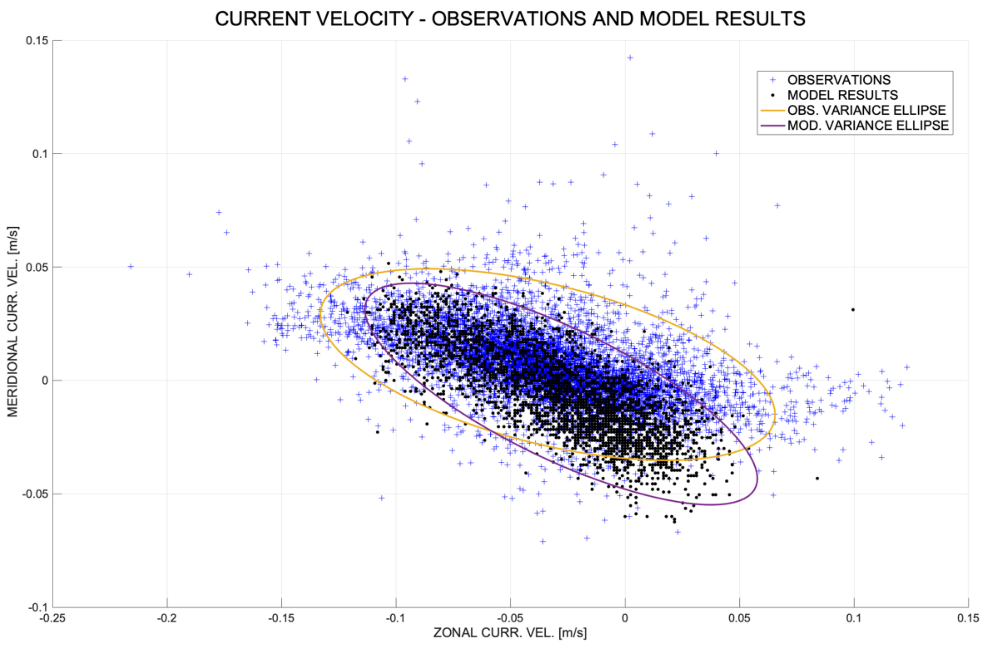
3.1.2. Water Currents

LADCP data were compared with the horizontal components of the water currents computed by the model for the nine sampling sites along the BC (see Figure 3B). The simulation run covering the period the data were collected, between 14 and 15 December 2016, allowed a direct comparison between the model results and observations. Nevertheless, due to the inaccuracies of the adopted forcing, parameterization and setup, the model performance levels were evaluated by comparing the measured data with the model values obtained at the two extremes during the three-hour temporal window the measurement was in. This time window was selected to account for both the errors in the reproduction of the tidal phases (see Section 3.1.1) and the possible inaccuracies in the adopted forcing and open boundary conditions.
In Table 2, the discrepancies between the model results and the observations were quantified by calculating the vectorial difference d between the observed and computed velocity.
For the sake of clarity, d is computed between observations (OBS in Table 2) and those model results with the best matching among the values computed within the three-hour temporal interval during which the measurement was carried out (MOD in Table 2). The vectorial distance d ranges from 0.03 m/s up to 0.27 m/s, with an average difference of 0.1 m/s. Considering the horizontal components of the current speed, for all the sampling stations, modeled and observed data are coherent and similar in terms of intensities, with differences of a few cm/s, with the exception of station 1, which is slightly mismatched.
These discrepancies are visualized in Figure 4A,B, where the modeled (red vectors in Figure 4 corresponding to MOD in Table 2) and observed currents (black vectors in Figure 4 corresponding to OBS in Table 2) are reported for each sampling station. The model results reproduce the BC current pattern with high accuracy especially for stations located inside the Ushuaia Bay (station 2 in panel A) and along the eastern sector of the BC (stations from 5 to 9 in panel B).
The dominance of the eastward flow with increasing speed intensity from west to east is easily recognized in both modeled and observed data. This pattern is also validated by the residual currents (grey vectors in Figure 4) obtained by the yearly averages of the horizontal velocity components, which confirm the prevalence of the eastward flow.
A further comparison between model results and observations was performed considering the near-bottom current speed data collected in Ushuaia Bay at 120 m depth (U station in Figure 3B) during 2017. Due to the mismatch between simulated and measuring periods, with model results obtained for the 2016 and observations collected during the 2017, only the statistical features of the modeled and observed current speeds were compared and analyzed. In Figure 5, the scatter plots of the horizontal components of the current speeds computed between May and December 2016 and measured between May and December 2017 at the U location are reported.
The two distributions are quite similar with a major axis directed east to west, a westward prevalent direction of the flow and with a very low variability along the north–south direction. Similar mean current speeds of 0.046 m/s and 0.042 m/s were obtained from observations and model results, respectively. Averages and standard deviations of the horizontal components were computed for both datasets. The results reveal a general match between the statistical features of the two distributions, with −0.033 m/s and 0.006 m/s versus −0.027 m/s and −0.004 m/s for observed and modeled averages of the zonal and meridional components of the current speed, respectively. Similar values were obtained for the standard deviations along the x and y-axis, with 0.04 m/s and 0.017 m/s for the observations, and 0.035 m/s and 0.02 m/s for the model results. The variance ellipses, defining the regions containing 95% of all observations and model results, were computed. In Figure 5, the iso-contours are depicted indicating a good matching between the two distributions, with the observed variance ellipse slightly more extended and less tilted with respect to the modeled one. Concluding, the model results reproduce with a good accuracy the main features of the near-bottom currents at station U, slightly underestimating the flow intensity.
The discrepancies between model results and measurements are generally small and can be associated with several sources of errors such as the inaccuracy in reproducing the bathymetry and geometric details of the measuring locations or the inaccuracies in the meteorological and oceanographic forcing and boundary conditions. Considering the scope of the paper, focusing on reproducing the transport time scales in the main part of the BC, the model performance levels, even if defined comparing data related to different years, can be considered as acceptable.

3.2. Simulations Results

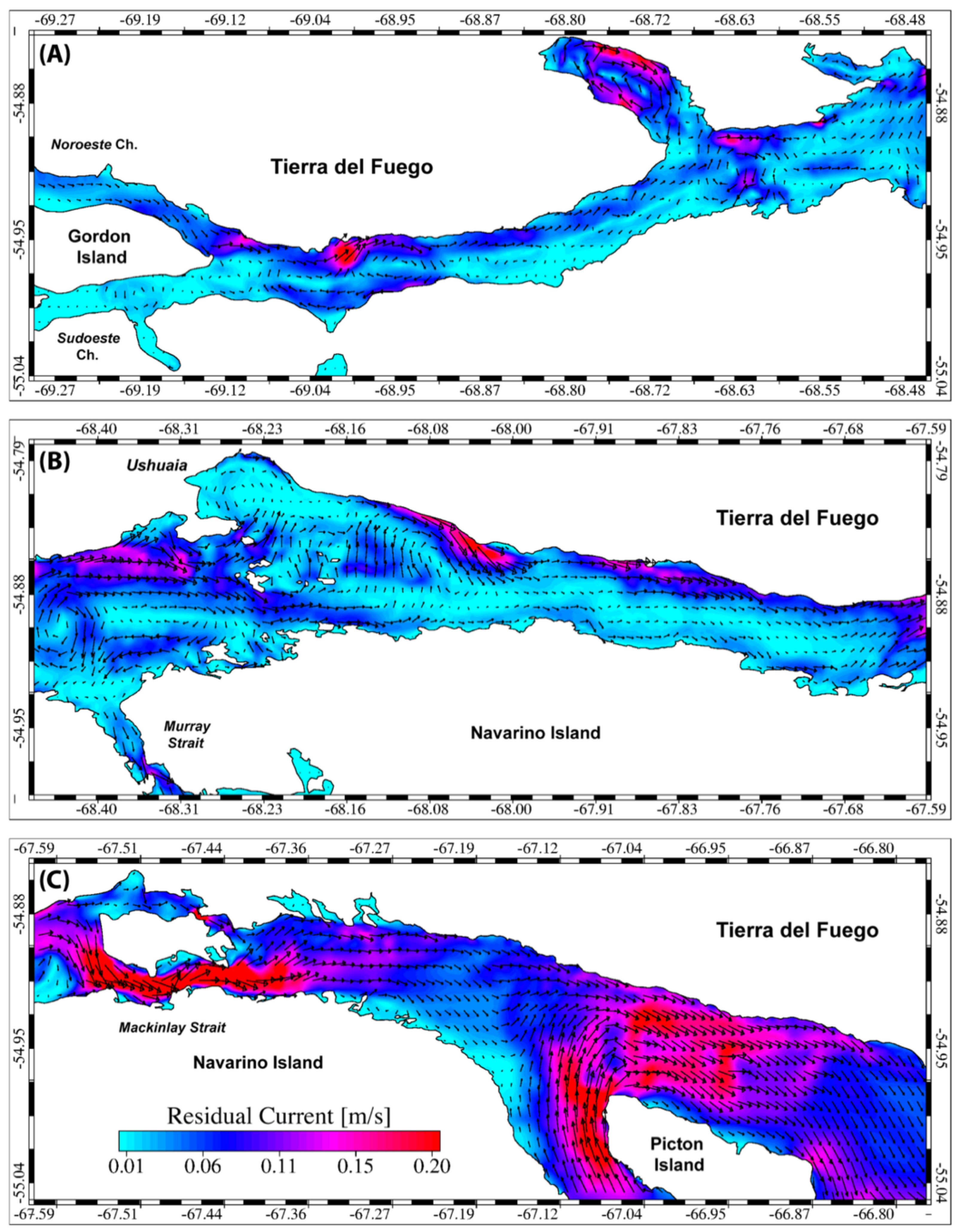
3.2.1. Water Circulation

The BC hydrodynamics were investigated throughout the computation of the residual water currents obtained by the time averaging of the horizontal components of the velocity fields [59,60]. The residual circulation is the main driver the spatial and temporal variability of transport time scales in semi enclosed basins [48,49]. In particular, it quantifies the mean flow by filtering the high frequency variability induced by both tidal and meteo-marine forcings. The same approach was followed with success in previous works by Cucco et al. (2006, 2009). Canu et al. (2012) aimed at analyzing the relationship between water circulation and transport time scales in lagoons and semi-enclosed basins under tidal and meteorological forcings. In Figure 6, the vertically averaged residual circulation computed for the whole simulated year is reported for the eastern (panel A), middle (panel B) and western sector (panel C) of the Central BC. The vertically averaged residual flow is mainly eastward along the whole channel with the presence of recirculation cells and calm water areas.
Water enters the BC from its western entrance, predominantly along the Noroeste branch (see Figure 6A), and flows eastwards along the northern side of the channel, generating residual anticlockwise circulation cells in correspondence with the abrupt bathymetric changes. The southern side of the channel is characterized by a low westward residual flow interspersed with calm water areas and recirculation cells (see Figure 6A).
In the central sector of the BC (see Figure 6B), the residual circulation is characterized by a more complex pattern due to the presence of morphological features such as Ushuaia Bay, a number of islands, and the Murray Channel. The residual flow, mainly eastward and with intensifications along the northern side of the channel, carries the waters into Ushuaia Bay from the West, through the dense net of shallow water passages cut across the archipelagos south of the bay. In agreement with previous studies [8,10,11], the circulation within the bay, characterized by an anticlockwise gyre along the western side and by a calm water area in its central part, is well reproduced by the model results. In the Murray Channel, the residual circulation is southward indicating that this passage promotes the outflow of the BC water. Beyond Ushuaia Bay, toward the east, the residual flow is mostly homogeneous in directions but with variation in the intensity fields from north to south, with minimum values in the middle of the channel.
An intensification of the residual flow is evident approaching the Mackinlay Strait where the highest residual currents are found (see Figure 6C). The eastern outflow is characterized by an intense and homogeneous residual current pattern carrying the BC waters toward the Atlantic Ocean across the passage between the main Tierra del Fuego and Picton islands. A further intensification of the water currents is observed in correspondence with the western tip of the Picton Island where the northward flow from the outer ocean and the BC outflow converges. The vertically averaged residual current intensities vary between a few cm/s in the calm water areas along the southern bank of the channel, to values higher than 0.35 m/s inside the Mackinlay Strait, with an average value around 0.1 m/s. We refer to Appendix C for a detailed overview of the variability of the residual flow along the vertical.

3.2.2. Water Fluxes

The computation of the inflow and outflow fluxes through the main openings, is necessary to define the cleaning capacity of semi-enclosed basins. In Table 3, the seasonally and yearly averaged water fluxes through the sections depicted in panel D of Figure 2 are reported.
The values indicate that the water masses enter in the BC from both the Northwest and Southwest branches (Sections S1 and S2) with a total flux varying between 8478 m3/s in autumn and 15,179 m3/s in summer and in spring (Section S3). The distribution of the total inflow between the two branches varies during the seasons with the Northwest contributing with percentages ranging from the 70% to 88% and the Southwest with values ranging from the 12% to 30% on the total flux through the BC. The amount of water entering in the middle sector of the BC (Section S5) partially outflow through the Murray Channel (Section S6) with average values ranging between 422 m3/s in autumn and 2773 m3/s in spring, corresponding to a percentage on the influx varying between the 5% in autumn and the 16% in spring.
Most of the water masses are carried eastward to the open ocean crossing the Mackinlay Strait (Section S9ab) with values ranging between 8121 m3/s during autumn and 13,430 m3/s in summer. Further east, the BC water converges to the Atlantic Ocean through the passage north of Picton Island, generating a total outflow ranging between 37,271 m3/s and 49,516 m3/s, depending on the season (Section S11). The seasonal variability of the residual exchanges is mainly due to the action of the westerly and southwesterly winds which promotes the eastward outflow inside the channel. We refer to Appendix D for a detailed description of the impact of the wind variability on the net exchanges.
On average the water flux intensities across the central BC varies between around 12,700 m3/s at its western entrance (Section S3) and around 11,200 m3/s at Mackinlay Strait (Section S9ab) with a secondary outflow of about 1500 m3/s across the Murray Channel (Sections S6).

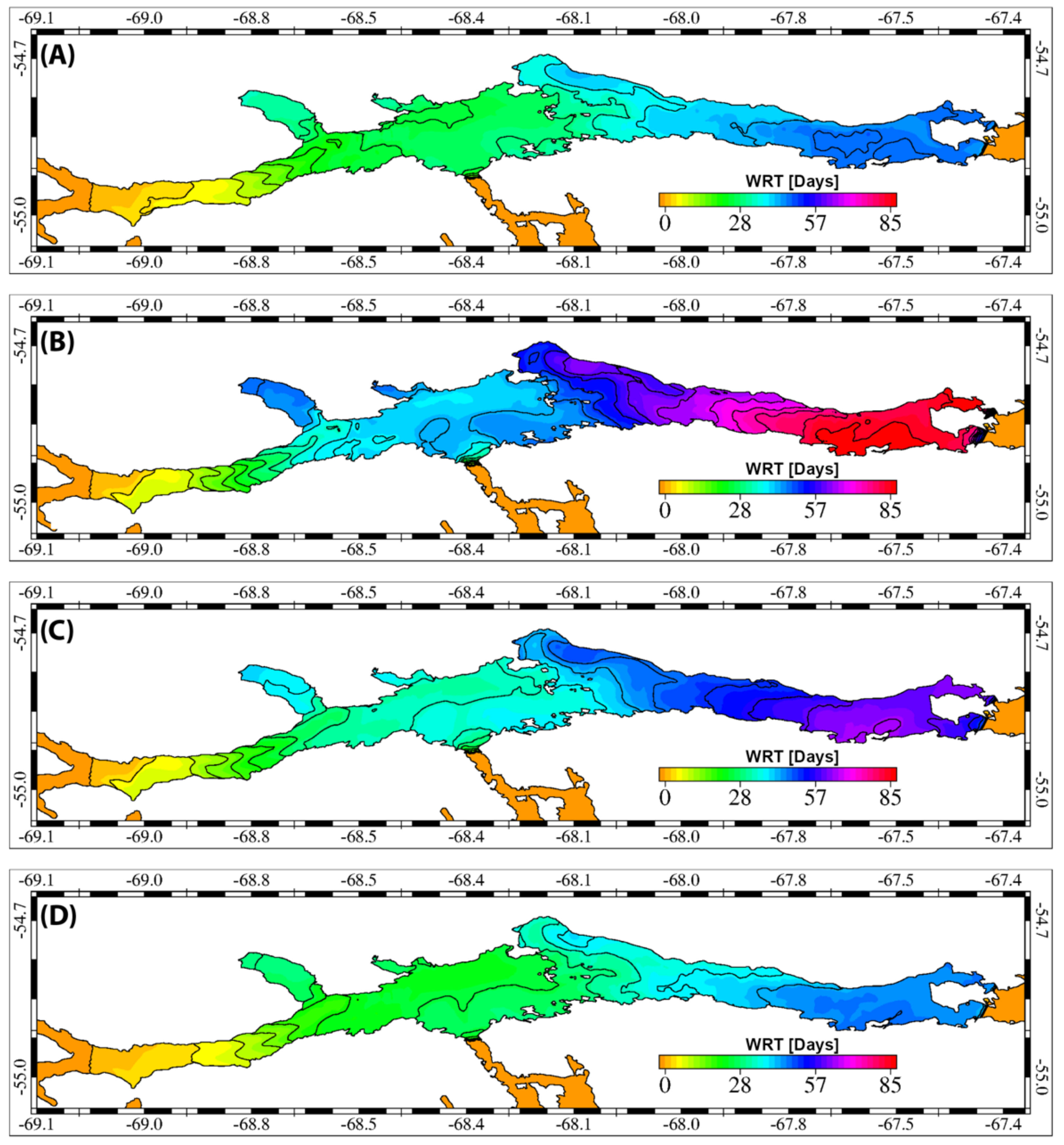
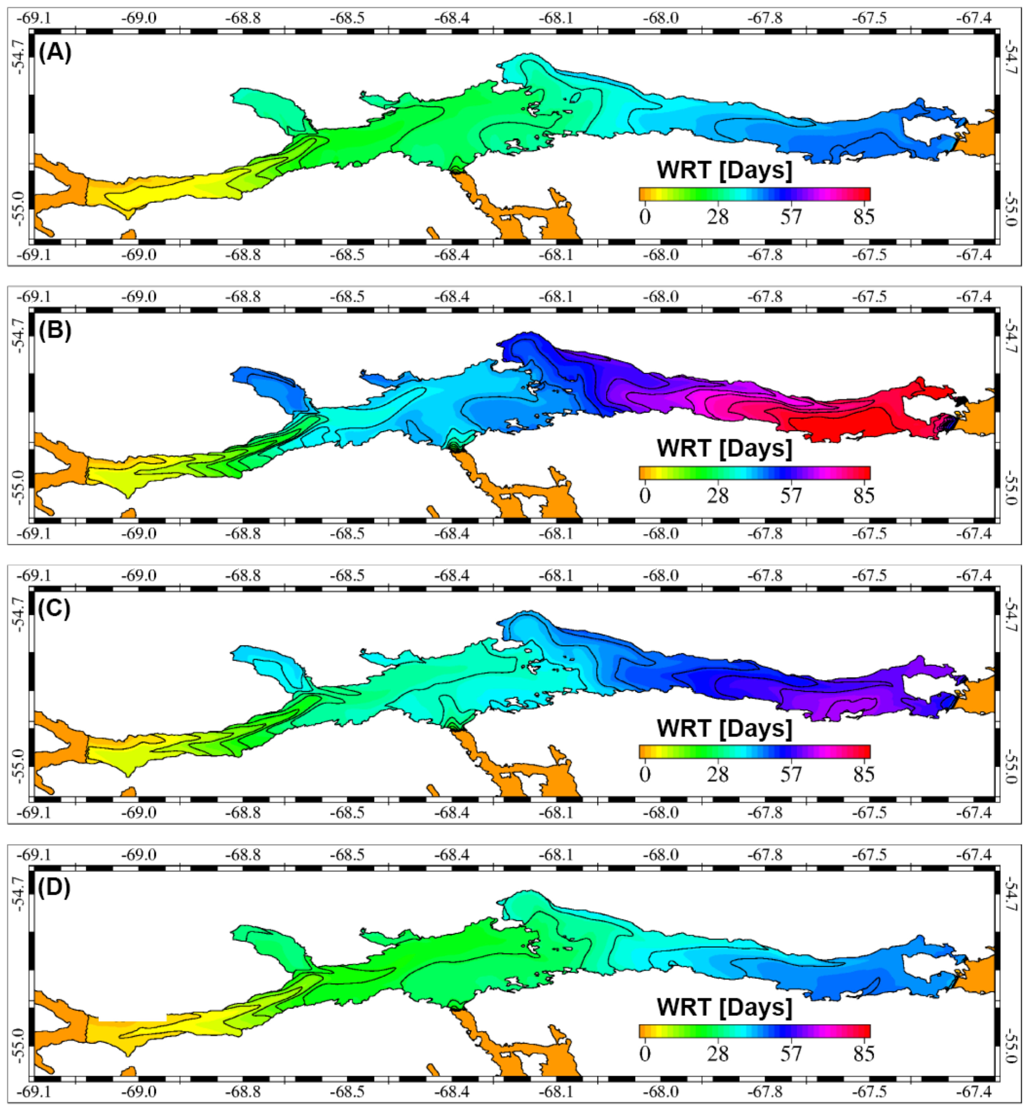
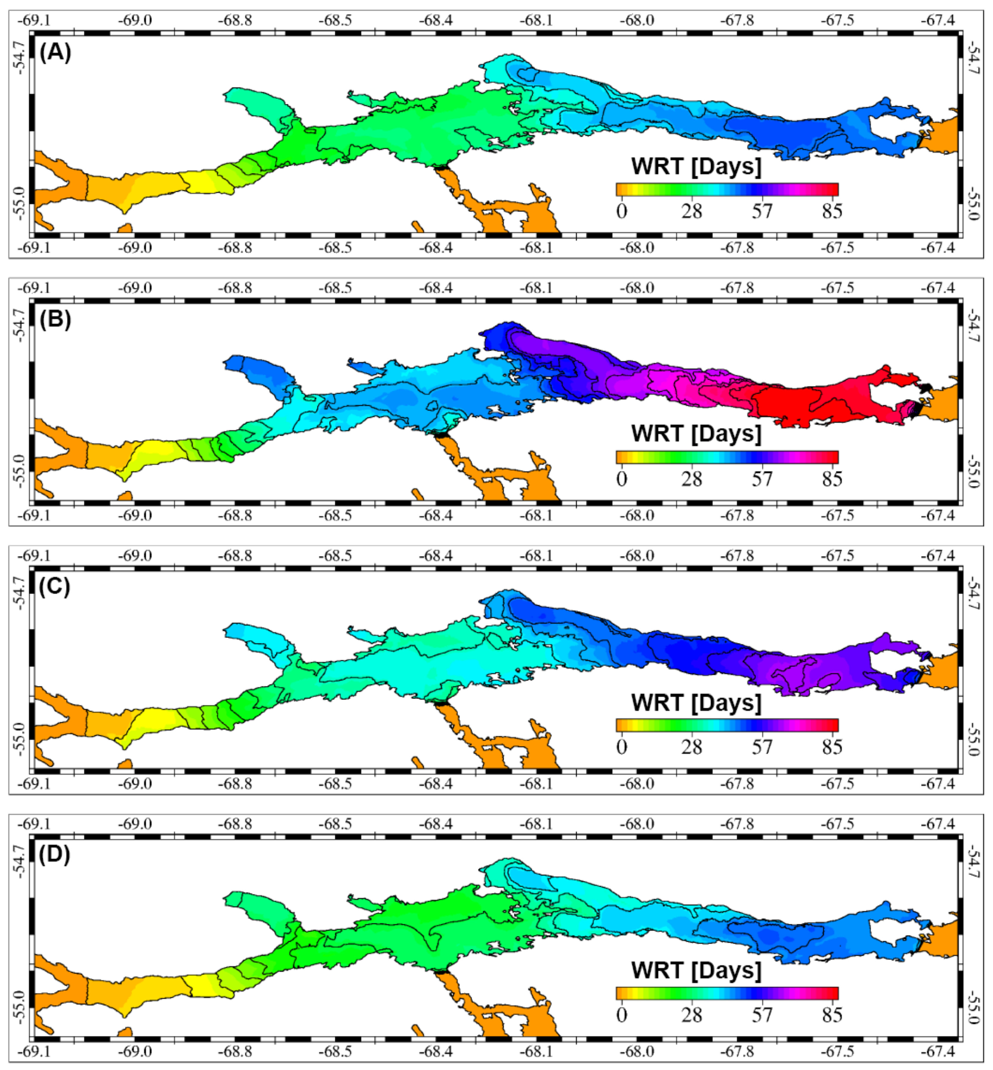
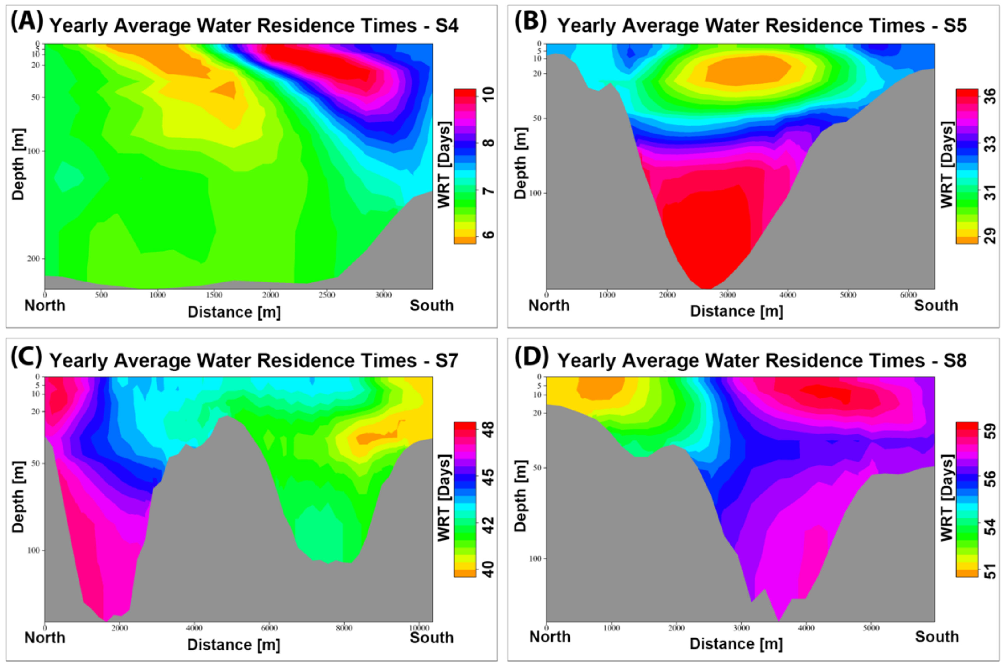
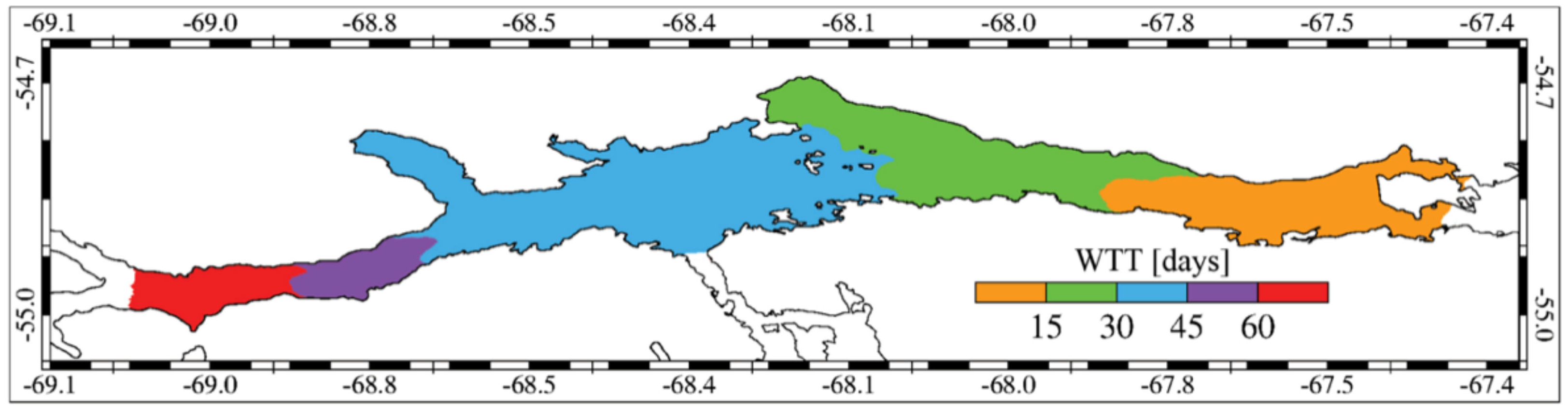
3.2.3. Transport Time Scales

We approximate the BC sector, comprised between sections S3, S6 and S9ab, as a rectilinear channel with an approximate volume V = 6.1 × 10 10   m3, corresponding to the yearly averaged water volume of the Central BC, and with a continuous water inflow and outflow through its openings equal to Q = 12 , 750   m3/s, which corresponds to the total yearly averaged outflows through section S9ab and S6 (see Table 3). Using these values as inputs for Equation (1), a yearly average turnover time (WTO) of about 55 days was estimated for the central BC.
Following the same approach, the seasonal WTO were computed obtaining values ranging from 46 days in summer up to 82 days in autumn with intermediate values of 61 and 44 days in winter and spring, respectively. These differences are mainly due to the changes in the water circulation intensities, i.e., the variation of the water levels is negligible if compared with the basin water depths, thus not affecting the total volume V.
In Figure 7, the vertically averaged water residence times (WRT), computed at seasonal time scale, are reported for the BC.
In all cases, the values are minimum at the west and maximum at the east as a consequence of the prevalent eastward flow. Minimum values are also found at the Murray Channel where the BC waters outflow to the open ocean. In all the panels, maximum values are found in proximity of the Mackinlay Strait, in correspondence with a shallow water bank along the southern side of the channel where the current intensity is generally reduced (see Figure 6). The west to east gradient is quite homogeneous except for the Ushuaia Bay where the WRT locally increases due to the peculiarity of the bay water circulation pattern (see Figure 6).
The lowest WRT values, with a basin average of 26 days and a maximum up to 53 days, are found in summer (see Figure 7A), when the fluxes across the channel are generally more intense and promote a higher flushing. On the contrary, the highest WRT, with a basin average of 43 days and a maximum of 95 days, are found in autumn (see Figure 7B) when water exchanges are low. Winter and spring seasons are characterized by intermediate WRT with basin averages varying between 34 and 30 days and maximum values between 67 and 53 days, respectively.
The spatial variability of the flushing features was analyzed in the three dimensions. In Figure 8 and Figure 9, the surface and bottom distribution of the seasonal WRT, corresponding to the model results obtained for the top and bottom layers, are depicted.
The main differences between surface and bottom WRT are observed in the western and central part of the domain where the bathymetric gradients are higher and the presence of a two layers residual flow was observed (see Appendix C). In particular, for all the seasons, in the western sector, a north to south positive component of the WRT gradient is found at the surface, while at the deeper layer, the gradient is mainly west to east, indicating the surface eastward flow along the northern BC side as the main dynamical feature promoting the flushing of this area. These differences are smoothed eastward along the channel up to the Mackinlay strait where the WRT is homogeneous along the vertical.
These features are well evidenced when analyzing the vertical distribution of the WRT. In Figure 10, the yearly WRT is displayed along a set of selected sections inside the channel (see Figure 2D) located in proximity of the western border (S4), in the middle channel (S5), in the Ushuaia Bay (S7) and in proximity of the western mouth (S8).
At the western border of the domain of interest, along Section S4 (see Figure 10A), the WRT is quite homogeneous, and most of the differences are found at the surface with values higher than 10 days on the southern side and values lower than few days on the north. This feature is smoothed while approaching eastward in the middle sector of the channel where the main differences in the flushing features are found along the vertical direction. An example is given by the distribution of the WRT along Section S5 (see Figure 10B) highlighting a higher cleaning capacity in the surface layers, with WRT values lower than 29 days, whereas a higher retention is found in the bottom layers, with WRT reaching 37 days. This section, characterized by steep bathymetric gradients, emphasizes the role of the residual flow (see Appendix C) in increasing the residence times of the waters in the bottom layers. In the eastern sector of the channel, the pattern of the WRT is characterized by lower values along the northern side and higher in the deeper part (see Figure 9). This feature is well represented by the distribution of the WRT computed along Section S8 (see Figure 10D) depicting a strong meridional gradient and a less intense vertical variation of the WRT, with the southern side characterized by WRT values higher at the surface than at the bottom.
An opposite pattern is found in Ushuaia Bay where the local circulation promotes an increase in the surface WRT along the northern coast with respect to the southern border. The main differences between the surface and bottom flushing features are found in the deeper part of the bay where the increase in the WRT is due both to the reduced local current intensity and to the direction of the flow that, moving northwest, carries the older water toward the inner bay. This is well evidenced by the distribution of the WRT along Section S7 located inside the bay (see Figure 10D) with the highest WRT values at the surface on the northern side and an increase in the retention time of the deeper waters at the bottom.
The seasonal surface and bottom WRT were extracted for stations from 1 to 6, located along the BC and in Ushuaia Bay (see Figure 3B) and the values reported in Table 4.
All the stations are located far from the southern coast and are characterized by a general increase in the WRT from the surface to the bottom layers. The differences vary among the seasons with the highest values, ranging between 6 and 9 days, found for stations 2 and 3 located inside the bay. Minimum differences are always found for station 6 located inside the Mackinlay Strait, where the shallow water area and the high flow intensity smash the vertical WRT gradient.
For each station, the relative increment of the WRT with the local water depth (D) was computed following a simple formula V R G = W R T b W R T s D   and the results reported in Table 4. This quantity provides an evaluation of the rate of increment of the residence time with the water depth allowing the identification of those areas where the local circulation is the main factor shaping the water retention features.
For all the seasons, the highest values, expressed in days per 100 m, are obtained for stations 2 and 3 located inside the Ushuaia Bay, thus confirming that the bottom waters in this area are relatively confined and potentially subjected to anoxic events and low ventilation efficiency.
Among the WRT and the WTO, a further a-dimensional quantity, the advection index (ADI), was computed following the simple formula A D I = W T O 2 * W R T a v g . Considering the methods adopted to compute the two transport time scales, in the case of a rectilinear channel with mono-directional and homogeneous flow, the relation WRTavg= WTO/2, is always satisfied. In this theoretical condition, the WRT increases linearly along the channel from 0 at the inlet, to maximum values, equal to WTO, at the outlet and, with a basin average value WRTavg, equal to the half of the WTO. In this case, the basin flushing features are dominated by the advection, whereas the diffusive processes, which could promote the trapping of the water masses, are absent. Therefore, the computation of ADI can be helpful to quantify the efficiency of the cleaning capacity for channel-type basins as the Beagle Channel. In particular, in the case A D I = 1 ,   the investigated domain can be considered as a channel with a mono directional and homogeneous flow characterized by a WTO which is equal to the time a tracer, initially released inside the channel, takes to completely flow out of the domain. On the other hand, ADI values lower than 1 indicate hydrodynamic patterns characterized by cleaning capacity deviating from the optimum, with both advection and diffusion processes determining the basin flushing feature. The ADI was computed for both seasonal and yearly distribution and the results, along with the main quantities to be considered when evaluating the BC flushing features, are reported in Table 5.
The ADI values highlight that the BC flushing features are, on average, 88% similar to the ones of a rectilinear channel with homogeneous and mono-directional flow. In this context, the advective processes are prevailing, with respect to the diffusive ones, on shaping the pattern of the flushing features inside the channel. As a consequence, the weight of the water trapping areas, as Ushuaia Bay, in determining the basin cleaning capacity is low, accounting for the 12%.
Therefore, assuming that, with a degree of similitude equal to 88%, the flushing features of the BC are typical of a rectilinear channel, the Lagrangian transport time scale or water transit times (WTT) can be easily assessed. In [48], the relation between the Lagrangian transport times scales, the WTT, and the Eulerian ones, the WRT, was analyzed in detail, evidencing that, in case of fully advection-dominated domain, the spatial distributions of the two times scales were reciprocal. Considering the results obtained from the ADI evaluation, the time a water particle takes to exit out of the BC can be estimated, with an accuracy of 88%, through the simple formula   W T T x , y = W R T m a x W R T x , y , with x and y indicating the location inside the channel.
Therefore, from values reported in Table 5, the WTT along the middle channel, where the flow is mainly dominated by advective processes, can vary, on average, from 67 days at the western entrance in correspondence with section S3 (see Figure 2D) up to few days in proximity of Mackinlay Strait at the eastern mouth.
In Figure 11, the WTT spatial distribution is reported as computed from the yearly vertically averaged WRT values.
The low resolution of the WTT distribution, characterized by a 15 days step, is adequate to the intrinsic inaccuracy of the calculation method. In fact, due to A D I 1 , the computed values are underestimated with respect to the ones obtained by using a particle tracking model (PTM). Nevertheless, the proposed rough zonation can be a helpful preliminary overview of the Lagrangian flushing features of the investigated basin, which can be subdivided into an eastern area characterized by WTT generally greater than 45 days, a central part with values varying between 15 to 30 days and a western sector with WTT always lower than 15 days.

4. Discussion and Conclusions

A high-resolution 3D hydrodynamic model based on the finite element method was applied to investigate the water circulation and the transport time scales in the Beagle Channel, a long and narrow interoceanic passage within the Tierra del Fuego archipelago in southern South America.
The presented numerical application provided the first large-scale comprehensive description of the general circulation and transport time scales in the Beagle Channel, a pristine marine environment in which many oceanographic aspects are still far from being fully understood. A set of fundamental information that may proof useful for a sustainable management of both marine resources and human activities in the Channel are provided.
The validation of the model with in situ data shows that the model reproduces with high accuracy the propagation of the tidal waves in the BC and the surrounding coastal areas.
Since the water circulation inside the channel was presumably not forced by tides only, the model results were also compared with surface current observations obtained for several stations along the channel and with near-bottom time-series of current velocity collected in Ushuaia Bay. For all the considered measuring stations, the computed horizontal components of the current speeds were appreciably coherent with the observations.
An improvement of the model validation procedure could be performed in the future, in case of the availability of a synoptic dataset of water currents and other oceanographic variables, which would allow a more detailed analysis of the model performance levels in reproducing specific features of the water circulation inside the channel.
Hence, the model has been applied to compute the residual water circulation inside the channel, which is one of the main aspects influencing the basin flushing features [59,60]. The obtained results highlight a circulation pattern characterized by a west-to-east (Pacific to Atlantic) residual flow with moderate intensity, low seasonal variability, minimum residual current speeds in autumn, and maximum in summer. A more complex pattern was found in Ushuaia Bay, where the residual flow is characterized by an anticlockwise circulation in the southwest edge of the bay, in concordance with previous studies in that particular location [10,11]. The seasonal variation of the residual flow is related to the time variability of the wind speed that modulates the intensity of the surface drag acting on the channel, with minimum values during the autumn and higher values during summer and spring.
The water infilling the BC enters its western sector mainly from the Northwest Branch and, to a lesser extent, from the Southwest Branch, with a total yearly average inflow around 12,700 m3/s. Then, it is carried eastwards along the central sector of the channel and through the Mackinlay Strait with a yearly average flux towards the open ocean around 11200 m3/s. Only a small percentage of the total BC water outflows across the Murray Channel, on the southern channel side, with a yearly average flux around 1500 m3/s. Finally, eastwards from the Mackinlay Strait, the BC water reaches the Atlantic Ocean through the passage north of Picton Island after being partially mixed with the open sea water coming from the passage south of the same island.
The flushing features of the Beagle Channel were analyzed at seasonal time scales through the computation of different quantities including the water turn-over time (WTO), the residence time (WRT) and the transit time (WTT).
The WTO was computed as a basin average without taking into account the spatial and temporal variability of the flow field and provides a theoretical and approximate estimate of the flushing features. WTO varied seasonally from 46 days in summer, when the water fluxes were more intense, up to 83 days in autumn, when the inflow and outflow were at minimum, and with a yearly average of 59 days.
On the contrary, the estimate of the WRT allowed us to analyze the spatial variability of the flushing features in the three dimensions. The results evidenced the same WTO seasonal trend, with the basin averages WRT lowest in summer, with 26 days, and highest in autumn, with 43 days, and with a yearly average value of 33 days. WRT values are at a minimum, around a few hours, at the western entrance and at a maximum, up to 95 days, at the eastern exit.
The WRT varies along the vertical direction with surface values generally lower on the northern side of the channel, and higher on the southern side. These differences are more pronounced in the western sector, where inversions of the residual flow directions are found across the channel sections. The Ushuaia Bay is characterized by a relative maximum of WRT especially in the deeper layers indicating this area can promote the trapping of the water masses.
This analysis, comparing the relative variation of the water flushing features at different water depths, allowed us to individuate the areas potentially subjected to water trapping phenomena generally leading to low ventilation and dissolved oxygen depletion. This is the case of the Ushuaia Bay, in which deeper parts are often subjected to such phenomena [11] and where the computed ratio between surface and deeper WRT values indicates a potential trapping of the water masses in the bottom layers.
The two times scales, WTO and WRT, were used to compute the ADI, an a-dimensional index that quantifies the efficiency of the cleaning capacity of channel-type basins. The obtained values evidenced that the BC flushing features were, on average, 88% comparable to the ones of a rectilinear channel with homogeneous and mono-directional flow. Specifically, A D I = 0.88   indicates that most of the BC, about 88%, is characterized by a mean rectilinear flow dominated by advective processes, which shapes the WRT spatial distribution as linearly increasing from the inlet (at the west) to the outlet (at the east). In the smaller portion of the channel, about 12%, the transport of the water masses is influenced mainly by diffusive processes, and in such areas (e.g., Ushuaia Bay), the water masses tend to be trapped. For this type of basin, a direct relation between the Eulerian (WRT) and the Lagrangian transport time scales (WTT) exists, which allows us to infer the WTT from the WRT spatial distribution [49]. The obtained values evidenced that the BC can be subdivided into a western area, characterized by WTT greater than 45 days, a central part with values varying between 15 and 30 days and an eastern sector with WTT always lower than 15 days.
The approach followed to compute the WTT is based on a strong assumption and can be used only to provide an approximated and averaged overview of the Lagrangian transport times scales inside the channel. This method cannot be used to estimate, with the necessary accuracy, the transit times of the water parcels from a specific location to the channel outlet, e.g., from the deep-water layers of the westerns sectors, where the residual currents are often westward. This level of information can be achieved only by applying a particle tracking model (PTM). Nevertheless, when the basin is characterized by a complex flow pattern, such as the one in the Ushuaia Bay or in the western sectors of the channel, even the adoption of PTM cannot be a proper solution. In fact, in this case, the interpretation of the Lagrangian trajectories is often difficult, both due to the so-called Lagrangian Chaos [61], which led a consistent fraction of the released particles to be retained indefinitely into the basin, and to the non-conservative features of the PTM method itself, which are not adequate to provide evaluations of the flushing features at basin scale. Therefore, the Eulerian approach we used, even if approximated, can provide a first insight into the Lagrangian transport time scales of the channel.
This study constitutes a necessary and preliminary step for the assessment of the carrying capacity of the marine system in relation to different types of human activities such as aquaculture, fisheries and tourism. However, future work is necessary to improve our understanding of this high latitude system, including the acquisition of new data (both Lagrangian and Eulerian measurements) along the entire channel and for longer periods; such research should be conducted in order to both acquire a more accurate overview of the BC general circulation and to provide an essential dataset for improving the future numerical model applications.
Among the possible applications of the present effort, several can be mentioned here: The WTO along with the mass flux estimation provide the basic information for implementing a box model approach to estimate the salt, nutrients or heavy metals budget in the channel, as conducted in other environments [62,63,64]. On the other hand, the computation of the WRT allows us to identify the areas of the domain characterized by higher sensibility to pollutants exposure in the case of contaminants released [65,66,67,68] and to identify those areas with water trapping features that can favor the accumulation of dispersed particles as larvae and eggs [69]. Finally, the WTT, providing an approximate quantification of the average time a water particle takes to exit out from the channel, can constitute helpful information to support the Satellite Aperture Radar procedures in case of maritime accidents or to be used for assessing the risk of impact of any oil spill events [70,71,72].

Supplementary Materials

The following supporting information can be downloaded at: https://www.mdpi.com/article/10.3390/jmse10070941/s1, Table S1: Observed (O) and Modeled (M) Amplitude (A) and Phase (P) expressed in m and degrees of the main harmonic constituents at the whole set of tidal stations analysed in D’Onofrio et al. (2016). Red characters indicate stations located inside the Beagle Channel and at its Eastern mouth along the southern Tierra del Fuego coastline.

Author Contributions

Conceptualization, A.C., J.M. and D.A.F.; methodology, A.C. and J.M.; software, A.C. and G.U.; validation, A.C., J.M. and H.F.; formal analysis, G.Q.; writing—original draft preparation, A.C.; writing—review and editing, A.C, J.M., G.Q, G.U. and D.A.F.; funding acquisition, A.C., D.A.F. and J.M. All authors have read and agreed to the published version of the manuscript.

Funding

This study was financed by the Project ‘Climate driven Changes in the Habitat Suitability of Marine Organisms’ (CLIMAR, ELAC2015/T01-0495) funded by the Network of the European Union, Latin America and the Caribbean Countries on Joint Innovation and Research Activities. Funding was also provided by Agencia Nacional de Promoción Científica y Tecnológica (PICT 2014/3106) and Consejo Nacional de Investigaciones Científicas y Técnicas (P-UE 2016: 22920160100077CO CADIC and PIP 440).

Data Availability Statement

In this research, primary data comes from model simulations performed using SHYFEM model Version 7.4.1, freely available at https://github.com/SHYFEM-model/shyfem/tree/master. All the model results, including data in figures and tables can be acquired by contacting the author via e-mail: andrea.cucco@cnr.it.

Acknowledgments

J. Martin wants to thank the officers and crew of the R/V ARA Puerto Deseado and Comando Naval Austral (Argentinian Navy) as well as all the scientific participants during field campaigns for their help at sea.

Conflicts of Interest

The authors declare no conflict of interest.

Appendix A. The Hydrodynamic Model

SHYFEM is a three-dimensional hydrodynamic model based on the finite element method, which resolves the shallow water equations integrated over each layer in their formulations with water levels and transports. The ocean is divided into single horizontal layers (z-layers), and the integrated equations on each layer are then solved. The equation system for a single layer l reads as:
U l t + u l U l t + v l U l t + w l U l t f V l   = g h l ζ x g h l ρ 0 x H l ζ ρ d z + h l ρ 0 p a x + A H 2 U l x 2 + 2 U l y 2 + z K l h l U l z + g h l η x g h l β ζ x
V l t + + u l V l t + v l V l t + w l U l t f U l   = g h l ζ y g h l ρ 0 y H l ζ ρ d z + h l ρ 0 p a y + A H 2 V l x 2 + 2 V l y 2 + z K l h l V l z + g h l η y g h l β ζ y
ζ t + l U l x + l U l x = 0
where l indicates the vertical layer, ( U l , V l ) the horizontal transports (integrated velocities over one layer) components in x and y directions for each layer, ( u l , v l ,   w l )   the velocity components, f the Coriolis parameter, p a   the atmospheric pressure,   g the gravitational constant, ζ   the sea level, ρ 0   the standard water density, ρ   the density anomaly, and ρ = ρ + ρ 0   the water density, τ   the internal stress term at the top and bottom of each layer, h l   the layer thickness, H l the depth of the bottom of the layer l , and A H   the horizontal eddy viscosity estimated following the Smagorinsky parameterization [73,74].
The GOTM (General Ocean Turbulence Model) turbulence closure model described in [75] was used for the computation of the vertical viscosity K l .
Momentum exchanges across the model layers are accounted by computing both the advective contribution and the vertical constituents of the diffusive terms z K l h l U l z   and   z K l h l V l z . The vertical velocities w are derived from the divergence of the horizontal flow field computed for each sub-surface layer in the continuity equations.
Wind and bottom friction terms, corresponding to the boundary conditions of the stress terms ( τ x , τ y ), are defined as:
τ x s u r f a c e = c D ρ a w i x w i x 2 + w i y 2
τ x b o t t o m = c B ρ 0 u L u L 2 + v L 2
τ y s u r f a c e = c D ρ a w i y w i y 2 + w i y 2
τ y b o t t o m = c B ρ 0 v L u L 2 + v L 2
with c D as the wind drag coefficient, c B the bottom friction coefficient, ρ a the air density ( w i x ,   w i y ) the wind velocity components and ( u L , v L ) the bottom velocity components.
Equilibrium tidal potential ( η ) and load tides are included as model forcing. The term η is computed as the sum of the tidal potential of each tidal constituent multiplied by the frequency-dependent elasticity factor [76], whereas the factor β accounts for the effects of load tides [61].
The hydrodynamic model is coupled with a 3D advection and diffusion numerical module to simulate the transport of both passive tracers and the salinity and temperature in the domain. The solute transport model is given as:
C l t + u l C l x + v l C l y + w l C l z = x K H C l x + y K H C l y + z K v C l z + E
where C l   is the concentration of any tracer (salinity, water temperature, or conservative tracer) at layer l, ( u l , v l ,   w l ) are the velocities, K H and K v   are the horizontal and vertical turbulent diffusion coefficients, respectively, and E is the source/loss term at the surface. A first-order explicit numerical scheme based on the TVD method was adopted to integrate in time the tracer advection and diffusion equation and a Smagorinsky formula was used to compute the horizontal tracer diffusion coefficients [73]. The GOTM turbulence closure model has been adopted for the vertical diffusivities. For the temperature, the source/loss term represents the heat source through the surface obtained by applying the AREG bulk algorithm [77].
In the case of salinity, the source/loss term represents the difference between evaporation and precipitation through the water surface (kg m−2 s−1) with evaporation rate determined by the bulk aerodynamic transfer method [78]. Details of numerical treatment and solved equations systems are reported in [28,79].

Appendix B. Tidal Propagation Dynamic

From the model results, the tidal maps of the M2-wave were computed for the BC and reported in Figure A1. The amplitude and phase maps indicate that tidal amplitudes tend to decrease from values around 0.6 m outside the channel, in the eastern mouth, to values around 0.4 m, inside the central part, with phases decreasing from east to west. The same analysis was carried out for the main diurnal constituent, the O1-wave indicating a similar propagation dynamic (not shown here) with amplitudes decreasing from east to west with values ranging between 0.2 m and 0.15 m along the channel. This behavior was similarly described by [50], confirming the accuracy of the model results in reproducing the main semidiurnal features of the tidal dynamic in the BC.
Figure A1. Modeled corange and cotidal maps for M2 in the BC and surroundings: corange lines in m (A) and cotidal lines in degrees (B).
Jmse 10 00941 g0a1

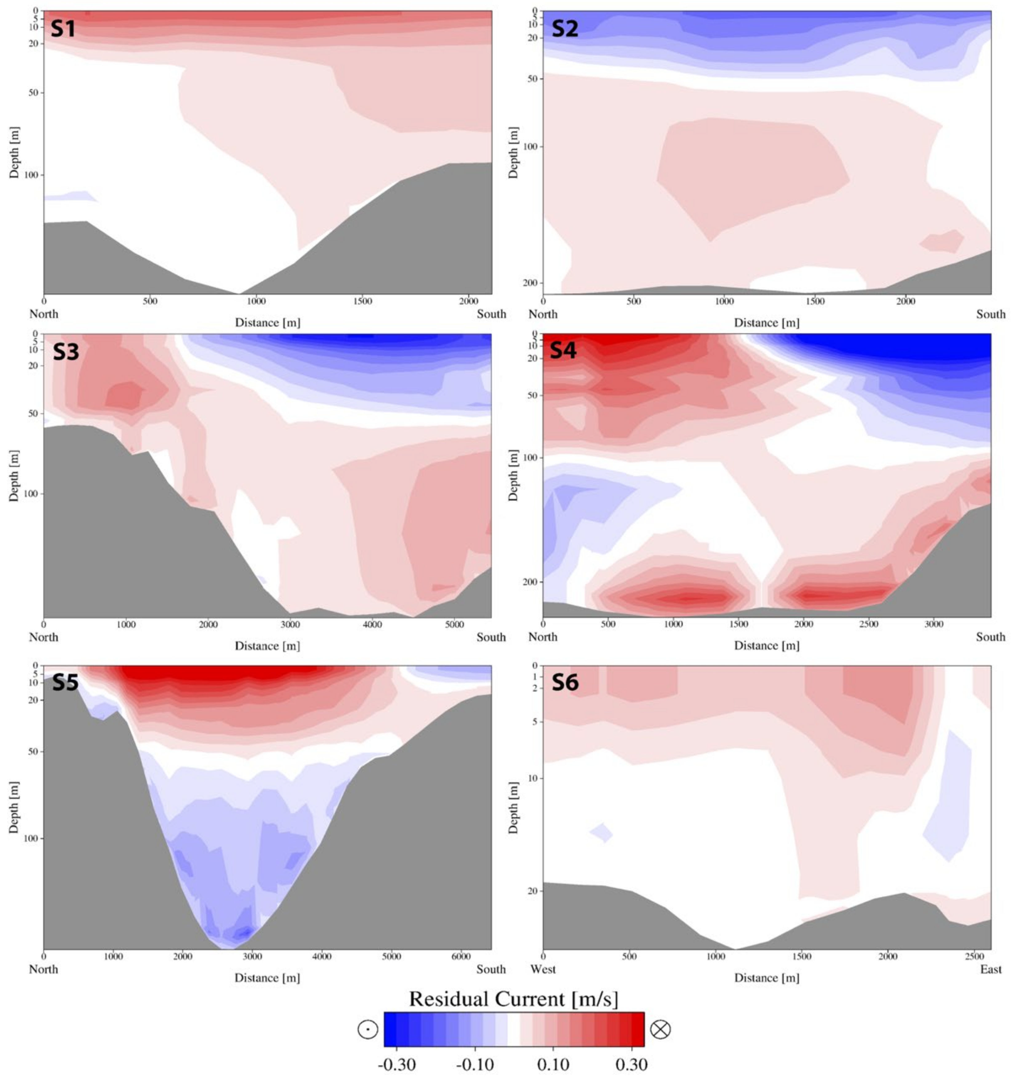
Appendix C. Residual Circulation

The variability of the residual flow along the vertical was investigated by computing the orthogonal component of the residual velocity field across each section depicted in Figure 2D. In Figure A2 and Figure A3 the results are reported.
Figure A2. Yearly residual flow intensity through the sections S1–S6 along the BC as reported in Figure 2. Positive values indicate an eastward flow, except for section S6, where positive values indicate a southward flow.
Jmse 10 00941 g0a2
Figure A3. Yearly residual flow intensity through the sections S7–S11 along the BC as reported in Figure 2. Positive values indicate an eastward flow.
Jmse 10 00941 g0a3
The results indicate that the residual flow is mainly eastward across the Northwest branch (section S1), while in the Southwest branch (section S2), an inversion of the flow field is denoted: westward at the surface and eastward in the deeper levels. At the entrance of the channel (section S3) the water from the Northwest branch moves eastward mainly along the northern coast and in the deeper layers while the westward residual flux outflowing through the Southwest channel is found at the surface mainly along the southern side. Sections located in the western sectors depict a more complex pattern, with section S4 intercepting the clockwise gyre characterized by an alternation of westward and eastward flows both along the meridional and vertical axis, and section S5 depicting an inversion of the residual flow with high intensities and prevalent eastward direction on the surface layers while lower speed values and westward direction on the deeper layers. Both sections are located in the channel area characterized by deep waters and strong bathymetric gradients that promote a two-layer dynamics with surface waters moving eastward, deeper, and more confined waters moving slowly and westward. This feature is smoothed approaching to the east where the shallower depths promote the vertical homogeneity of the flow field.
Section S6, in correspondence with the Murray Channel, depicts a vertically homogeneous southward residual flow indicating the outflow of the BC waters through this passage occurs along the whole water column.
Section S7 crosses to the east of Ushuaia Bay, highlighting the peculiarity of the flow in this area. Within the bay, the northern part of section S7, an intense and surface residual outflow is found in proximity of the northern side, whereas at the deeper layers, the direction of the residual flow is opposite. This feature is in line with the LADCP measurements (see Section 3.1.2) and previous studies [9,11,12,13], indicating the bay waters outflow at the surface along the northern coast and the inflow of the BC waters in correspondence with the deeper layers.
Along the eastern, shallower sectors (sections from S8 to S11), the residual flow is mostly homogeneous in vertical, eastward across sections S8, S9a and S11 and north-westward across section S10 highlighting the BC waters outflowing and the ocean water inflowing dynamic previously described.

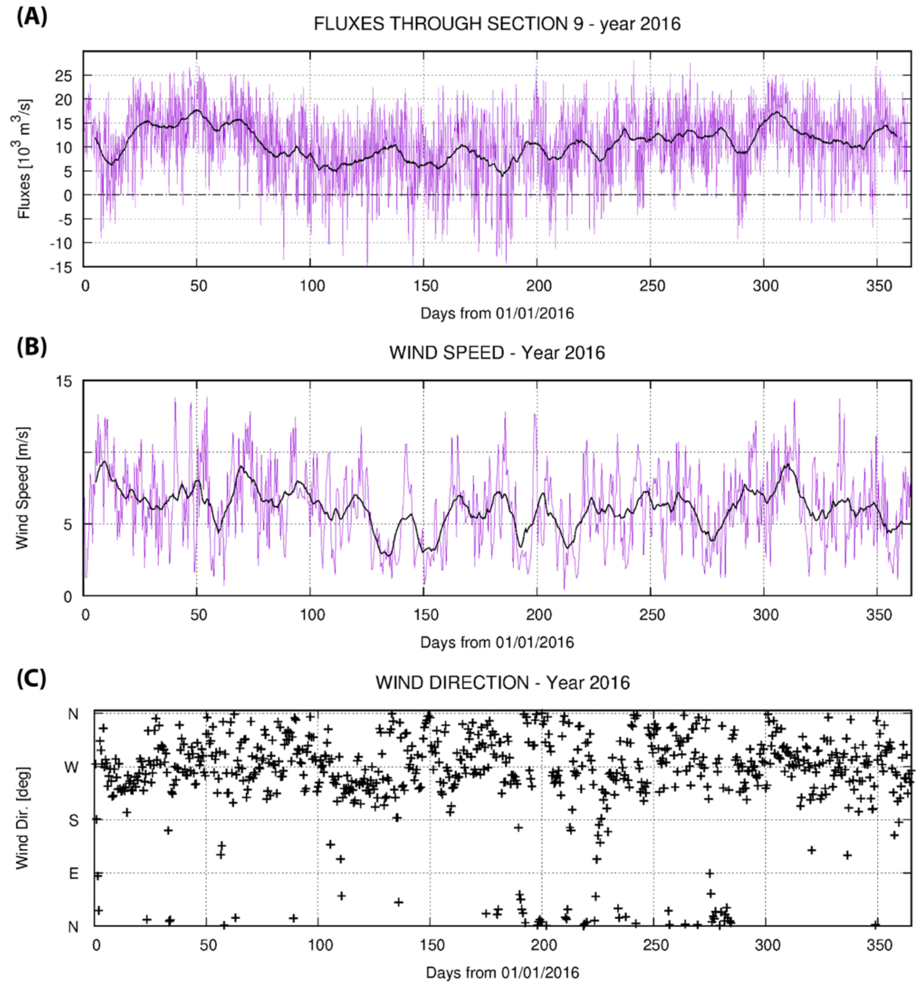
Appendix D. Water Fluxes

In Figure A4, the fluxes through Section S9ab computed for the whole simulated year 2016 are reported along with the wind speeds and directions obtained from the adopted meteorological forcing in correspondence with the Ushuaia Bay.
Figure A4. Fluxes through Section S9ab during the whole of 2016 (A), three-hour of data (colored line) and ten-day averages (black continuous line). Positive values indicate an eastward flow, while negatives indicate a westward one. Wind speed (B) and directions (C) at Ushuaia Bay are obtained from the adopted meteorological forcing dataset for the entire year of 2016. In (B), colored line indicates the original dataset at semidiurnal frequency, and the black line indicates the ten-day-averaged values.
Jmse 10 00941 g0a4
Most of the dataset (colored line in Figure A4A) consists of positive values indicating a prevailing eastward outflow through Mackinlay Strait. Westward inflows occur sporadically mainly in autumn and winter periods. The temporal variation of the water fluxes is modulated by the tides, at semidiurnal frequency, and by the atmospheric and oceanographic forcing, at lower frequencies, from weekly to seasonal.
The seasonal variation of the average outflows reported in Table 3 is well reproduced by the ten days averaged fluxes depicted by the black line in Figure A4A, with maximum values of outflow occurring during summer, decreasing in autumn and slowly increasing again during winter and spring. A similar behavior is found in the ten-day wind speed averages depicted in Figure A4B, with higher values during summer, a reduction in intensities in autumn and a further increment in the wind speed during winter and spring. This similitude led us to consider the wind as one of the main factors modulating the variability of the BC water circulation and outflows. During the whole simulated period, the wind direction is mainly varying between northwest and southwest, with westerly and southwesterly winds prevailing among other directions in terms of both frequency and intensity, confirming this forcing promotes the eastward flow within the BC.

References

  1. Bujalesky, G.G. The flood of the Beagle Valley (11000 YR B.P.), Tierra del Fuego. An. Inst. Patagonia 2011, 39, 5–21. [Google Scholar] [CrossRef] [Green Version]
  2. Antezana, T. Hydrographic features of Magellan and Fuegian inland passages and adjacent subantarctic waters. Sci. Mar. 1999, 63, 23–34. [Google Scholar] [CrossRef]
  3. Acha, E.M.; Mianzan, H.W.; Guerrero, R.A.; Favero, M.; Bava, J. Marine fronts at the continental shelves of austral South America: Physical and ecological processes. J. Mar. Syst. 2004, 44, 83–105. [Google Scholar] [CrossRef]
  4. Guihou, K.; Piola, A.R.; Palma, E.D.; Chidichimo, M.P. Dynamical connections between large marine ecosystems of austral South America based on numerical simulations. Ocean. Sci. 2020, 16, 271–290. [Google Scholar] [CrossRef] [Green Version]
  5. Bown, F.; Rivera, A.; Zenteno, P.; Bravo, C.; Cawkwell, F. First Glacier Inventory and Recent Glacier Variation on Isla Grande de Tierra Del Fuego and Adjacent Islands in Southern Chile. In Global Land Ice Measurements from Space; Springer: Berlin/Heidelberg, Germany, 2014; pp. 661–674. [Google Scholar] [CrossRef]
  6. Iturraspe, R.; Sottini, R.; Schroeder, C.; Escobar, J. Hidrología y variables climáticas del territorio de tierra del fuego. Inf. Básica Contrib. Científica CADIC 1989, 7, 201. [Google Scholar]
  7. D’Onofrio, E.; Orsi, A.; Locarnini, R. Estudio de marea en la costa de Tierra del Fuego. Inf. Técnico Serv. Hi-Drog. Nav. 1989, 49, 81p. [Google Scholar]
  8. Balestrini, C.F.; Vinuesa, J.; Speroni, J.; Lovrich, G.; Mattenet, C.; Cantú, C.; Medina, P. Estudio de las Corrientes Marinas en los Alrededores de la Península Ushuaia; Comunicación Científica N°10; CADIC—Centro Austral de Investigaciones Científicas: Ushuaia, Argentina, 1990. [Google Scholar]
  9. Speroni, J.O.; Dragani, W.C.; Mazio, C.A. Mediciones de Corriente en Paso Mackinlay, Canal Beagle, Tierra del Fuego, Departamento Oceanografia, Informe Tecnico 1/3. 2003. Available online: https://www.researchgate.net/publication/312613566_Simulacion_de_corrientes_en_el_Canal_Beagle_y_Bahia_Ushuaia_mediante_un_modelo_bidimensional (accessed on 1 March 2020).
  10. Balestrini, C.; Manzella, G.; Lovrich, G. Simulación de Corrientes en el Canal Beagle y Bahía Ushuaia, Mediante un Modelo Bidimensional. Servicio de Hidrografía Naval; Informe Técnico 98; Departamento de Oceanografia: Ushuaia, Argentina, 1998; p. 58. [Google Scholar]
  11. Flores-Melo, X.; Martín, J.; Kerdel, L.; Bourrin, F.; Colloca, C.B.; Menniti, C.; Durrieu de Madron, X.D. Particle Dynamics in Ushuaia Bay (Tierra del Fuego)-Potential Effect on Dissolved Oxygen Depletion. Water 2020, 12, 324. [Google Scholar] [CrossRef] [Green Version]
  12. Giesecke, R.; Martín, J.; Piñones, A.; Höfer, J.; Garcés-Vargas, J.; Flores-Melo, X.; Alarcón, E.; de Madron, X.D.; Bourrin, F.; González, H.E. General hydrography of the beagle channel, a subantarctic interoceanic passage at the southern tip of South America. Front. Mar. Sci. 2021, 8, 621822. [Google Scholar] [CrossRef]
  13. Giarratano, E.; Amin, O.A. Heavy metals monitoring in the southernmost mussel farm of the world (Beagle Channel, Argentina). Ecotoxicol. Environ. Saf. 2010, 73, 1378–1384. [Google Scholar] [CrossRef]
  14. Gil, M.; Torres, A.; Amin, O.; Esteves, J. Assessment of recent sediment influence in an urban polluted subantarctic coastal ecosystem. Beagle Channel (Southern Argentina). Mar. Pollut. Bull. 2011, 62, 201–207. [Google Scholar] [CrossRef]
  15. Biancalana, F.; Dutto, S.; Berasategui, A.A.; Kopprio, G.; Hoffmeyer, M.S. Mesozooplankton assemblages and their relationship with environmental variables: A study case in a disturbed bay (Beagle Channel, Argentina). Environ. Monit. Assess. 2014, 186, 8629–8647. [Google Scholar] [CrossRef] [PubMed]
  16. Fabião, J.P.F.; Rodrigues, M.F.G.; Fortunato, A.B.; Jacob, J.M.Q.D.B.; Cravo, A.M.F. Water exchanges between a multi-inlet lagoon and the ocean: The role of forcing mechanisms. Ocean Dyn. 2016, 66, 173–194. [Google Scholar] [CrossRef]
  17. Malhadas, M.S.; Neves, R.J.; Leitão, P.C.; Silva, A. Influence of tide and waves on water renewal in Óbidos Lagoon, Portugal. Ocean Dyn. 2010, 60, 41–55. [Google Scholar] [CrossRef]
  18. Oliveira, A.; Rodrigues, M.; Fortunato, A.B.; Guerreiro, M. Impact of seasonal bathy- metric changes and inlet morphology on the 3D water renewal and residence times of a small coastal stream. J. Coast. Res. 2011, 64, 1555–1559. [Google Scholar]
  19. Ranjbar, M.H.; Zaker, N.H. Numerical modeling of general circulation, thermohaline structure, and residence time in Gorgan Bay, Iran. Ocean Dyn. 2017, 68, 35–46. [Google Scholar] [CrossRef]
  20. Howarth, R.; Swaney, D.P.; Butler, T.J.; Marino, R. Rapid communication: Climatic control on eutrophication of the Hudson river estuary. Ecosystems 2000, 3, 210–215. [Google Scholar] [CrossRef]
  21. Wang, H.; Chen, Q.; Hu, K.; La Peyre, M.K. A modeling study of the impacts of Mississippi river diversion and sea-level rise on water quality of a deltaic estuary. Estuar. Coasts 2017, 40, 1028–1054. [Google Scholar] [CrossRef]
  22. Riccialdelli, L.; Newsome, S.D.; Fogel, M.L.; Fernández, D.A. Trophic interactions and food web structure of a subantarctic marine food web in the beagle channel: Bahía Lapataia, Argentina. Polar Biol. 2016, 40, 807–821. [Google Scholar] [CrossRef]
  23. Riccialdelli, L.; Becker, Y.; Fioramonti, N.; Torres, M.; Bruno, D.; Rey, A.R.; Fernández, D. Trophic structure of southern marine ecosystems: A comparative isotopic analysis from the Beagle Channel to the oceanic Burdwood Bank area under a wasp-waist assumption. Mar. Ecol. Prog. Ser. 2020, 655, 1–27. [Google Scholar] [CrossRef]
  24. Zhan, P.; Krokos, G.; Langodan, S.; Guo, D.; Dasari, H.; Papadopoulos, V.P.; Lermusiaux, P.; Knio, O.; Hoteit, I. Coastal cir-culation and water transport properties of the red sea project lagoon. Ocean. Model. 2021, 161, 101–791. [Google Scholar] [CrossRef]
  25. Tartinville, B.; Deleersnijder, E.; Rancher, J. The water residence time in the Mururoa atoll lagoon: Sensitivity analysis of a three-dimensional model. Coral Reefs 1997, 16, 193–203. [Google Scholar] [CrossRef] [Green Version]
  26. Yahel, G.; Post, A.F.; Fabricius, K.; Marie, D.; Vaulot, D.; Genin, A. Phytoplankton distribution and grazing near coral reefs. Limnol. Oceanogr. 1998, 43, 551–563. [Google Scholar] [CrossRef]
  27. Bruno, D.O.; Victorio, M.F.; Acha, E.M.; Fernández, D.A. Fish early life stages associated with giant kelp forests in sub-Antarctic coastal waters (Beagle Channel, Argentina). Polar Biol. 2017, 41, 365–375. [Google Scholar] [CrossRef]
  28. Umgiesser, G.; Canu, D.M.; Cucco, A.; Solidoro, C. A finite element model for the Venice lagoon: Development, set up, calibration and validation. J. Mar. Syst. 2004, 51, 123–145. [Google Scholar] [CrossRef]
  29. Bellafiore, D.; Umgiesser, G. Hydrodynamic coastal processes in the North Adriatic investigates with a 3D finite element model. Ocean Dyn. 2010, 60, 255–273. [Google Scholar] [CrossRef]
  30. Cucco, A.; Sinerchia, M.; Ribotti, A.; Olita, A.; Fazioli, L.; Sorgente, B.; Perilli, A.; Borghini, M.; Schroeder, K.; Sorgente, R. A high-resolution real-time forecasting system for predicting the fate of oil spills in the strait of Bonifacio (western Mediter-Ranean Sea). Mar. Pollut. Bull. 2012, 64, 1186–1200. [Google Scholar] [CrossRef]
  31. Bajo, M.; Ferrarin, C.; Dinu, I.; Umgiesser, G.; Stanica, A. The water circulation near the Danube delta and the Romanian coast modelled with finite elements. Cont. Shelf Res. 2014, 78, 62–74. [Google Scholar] [CrossRef]
  32. Cucco, A.; Quattrocchi, G.; Satta, A.; Antognarelli, F.; De Biasio, F.; Cadau, E.; Umgiesser, G.; Zecchetto, S. Predictability of wind-induced sea surface transport in coastal areas. J. Geophys. Res. Oceans 2016, 121, 5847–5871. [Google Scholar] [CrossRef] [Green Version]
  33. Ferrarin, C.; Davolio, S.; Bellafiore, D.; Ghezzo, M.; Maicu, F.; McKiver, W.; Drofa, O.; Umgiesser, G.; Bajo, M.; De Pascalis, F.; et al. Cross-scale operational oceanography in the Adriatic Sea. J. Oper. Oceanogr. 2019, 12, 86–103. [Google Scholar] [CrossRef]
  34. Umgiesser, G.; Ferrarin, C.; Cucco, A.; De Pascalis, F.; Bellafiore, D.; Ghezzo, M.; Bajo, M. Comparative hydrodynamics of 10 mediterranean lagoons by means of numerical modeling. J. Geophys. Res. Oceans 2014, 119, 2212–2226. [Google Scholar] [CrossRef]
  35. IOC, IHO, and BODC, Centenary Edition of the GEBCO Digital Atlas, Published on CD-ROM on Behalf of the Intergovernmental Oceanographic Commission and the International Hydrographic Organization as Part of the General Bathymetric Chart of the Oceans; British Oceanographic Data Centre, Liverpool. 2003. Available online: https://www.gebco.net (accessed on 1 March 2020).
  36. Smith, S.D. Wind stress and turbulence over a flat ice floe. J. Geophys. Res. Earth Surf. 1972, 77, 3886–3901. [Google Scholar] [CrossRef]
  37. Madec, G.; Delecluse, P.; Imbard, M.; Levy, C. OPA 8.1 Ocean General Circulation Model Reference Manual; Technical Report LODYC/IPSL Note 11; French National Centre for Scientific Research: Paris, France, 1998. [Google Scholar]
  38. Berrisford, P.; Kållberg, P.; Kobayashi, S.; Dee, D.; Uppala, S.; Simmons, A.J.; Poli, P.; Sato, H. Atmospheric conservation properties in ERA-interim. Q. J. R. Meteorol. Soc. 2011, 137, 1381–1399. [Google Scholar] [CrossRef]
  39. Egbert, G.; Bennett, A.F.; Foreman, M.G.G. TOPEX/POSEIDON tides estimated using a global inverse model. J. Geophys. Res. Earth Surf. 1994, 99, 24821–24852. [Google Scholar] [CrossRef] [Green Version]
  40. Egbert, G.D.; Erofeeva, S.Y. Efficient Inverse Modeling of Barotropic Ocean Tides. J. Atmos. Ocean. Technol. 2002, 19, 183–204. [Google Scholar] [CrossRef] [Green Version]
  41. Fernandez, D.A.; Ciancio, J.; Ceballos, S.; Rossi, C.R.; Pascual, M. Salmón Chinook en el Parque Nacional Tierra del Fuego: Un Evento Aislado o el Inicio de un Proceso de Colonización; Technical Report, Informe Técnico Salmon Chinook PNTDF; CADIC-Centro Austral de Investigaciones Cientificas: Ushuaia, Argentina, 2007. [Google Scholar]
  42. Takeoka, H. Fundamental concepts of exchange and transport time scales in a coastal sea. Cont. Shelf Res. 1984, 3, 311–326. [Google Scholar] [CrossRef]
  43. Monsen, N.E.; Cloern, J.E.; Lucas, L.V.; Monismith, S.G. A comment on the use of flushing time, residence time, and age as transport time scales. Limnol. Oceanogr. 2002, 47, 1545–1553. [Google Scholar] [CrossRef] [Green Version]
  44. Delhez, E.J.M.; Heemink, A.W.; Deleersnijder, E. Residence time in a semi-enclosed domain from the solution of an adjoint problem. Estuar. Coast. Shelf Sci. 2004, 61, 691–702. [Google Scholar] [CrossRef]
  45. Jouon, A.; Douillet, P.; Ouillon, S.; Fraunié, P. Calculations of hydrodynamic time parameters in a semi-opened coastal zone using a 3D hydrodynamic model. Cont. Shelf Res. 2006, 26, 1395–1415. [Google Scholar] [CrossRef]
  46. Liu, W.-C.; Chen, W.-B.; Kuo, J.-T.; Wu, C. Numerical determination of residence time and age in a partially mixed estuary using three-dimensional hydrodynamic model. Cont. Shelf Res. 2008, 28, 1068–1088. [Google Scholar] [CrossRef]
  47. de Brye, B.; de Brauwere, A.; Gourgue, O.; Delhez, E.J.; Deleersnijder, E. Water renewal timescales in the scheldt estuary. J. Mar. Syst. 2012, 94, 74–86. [Google Scholar] [CrossRef]
  48. Cucco, A.; Umgiesser, G.; Ferrarin, C.; Perilli, A.; Canu, D.M.; Solidoro, C. Eulerian and Lagrangian transport time scales of a tidal active coastal basin. Ecol. Model. 2009, 220, 913–922. [Google Scholar] [CrossRef]
  49. Cucco, A.; Umgiesser, G. The trapping index: How to integrate the eulerian and the lagrangian approach for the compu-tation of the transport time scales of semi-enclosed basins. Mar. Pollut. Bull. 2015, 98, 210–220. [Google Scholar] [CrossRef] [PubMed]
  50. D’Onofrio, E.E.; Oreiro, F.A.; Grismeyer, W.H.; Fiore, M.M.E. Accurate astronomical tide predictions calculated from satellite altimetry and coastal observations for the area of isla grande de tierra del fuego, Isla de los Estados and Beagle Channel. GEOACTA 2016, 40, 60–75. [Google Scholar]
  51. Visbeck, M. Deep velocity profiling using lowered acoustic doppler current profilers: Bottom track and inverse so-lutions. J. Atmos. Ocean. Technol. 2002, 19, 794–807. [Google Scholar] [CrossRef]
  52. Thurnherr, A.M. A practical assessment of the errors associated with full-depth LADCP profiles obtained using Teledyne RDI workhorse acoustic doppler current profilers. J. Atmos. Ocean. Technol. 2010, 27, 1215–1227. [Google Scholar] [CrossRef]
  53. Cera, T.B. Tidal Analysis Program in Python (TAPPY). Software Repository. 2011. Available online: http://tappy.sourceforge.net (accessed on 1 March 2020).
  54. Foreman, M.G.G.; Henry, R.F.; Walters, R.A.; Ballantyne, V.A. A finite element model for tides and resonance along the north coast of British Columbia. J. Geophys. Res. Earth Surf. 1993, 98, 2509–2531. [Google Scholar] [CrossRef]
  55. Tsimplis, M.N.; Proctor, R.; Flather, R.A. A two-dimensional tidal model for the Mediterranean sea. J. Geophys. Res. Ocean. 1995, 100, 16223–16239. [Google Scholar] [CrossRef]
  56. Ferrarin, C.; Roland, A.; Bajo, M.; Umgiesser, G.; Cucco, A.; Davolio, S.; Buzzi, A.; Malguzzi, P.; Drofa, O. Tide-surge-wave modelling and forecasting in the Mediterranean Sea with focus on the Italian coast. Ocean. Model. 2013, 61, 38–48. [Google Scholar] [CrossRef] [Green Version]
  57. Arabelos, D.N.; Papazachariou, D.Z.; Contadakis, M.E.; Spatalas, S.D. A new tide model for the Mediterranean sea based on altimetry and tide gauge assimilation. Ocean. Sci. 2011, 7, 429–444. [Google Scholar] [CrossRef] [Green Version]
  58. Yanagi, T. Fundamental study on the tidal residual circulation—I. J. Oceanogr. 1976, 32, 199–208. [Google Scholar] [CrossRef]
  59. Souto, C.; Gil Coto, M.; Fariña-Busto, L.; Perez, F.F. Modeling the residual circulation of a coastal embayment affected by wind-driven upwelling: Circulation of the ría de vigo (NW Spain). J. Geophys. Res. Earth Surf. 2003, 108, 3340. [Google Scholar] [CrossRef] [Green Version]
  60. Meyers, S.D.; Luther, M.E. A numerical simulation of residual circulation in tampa bay. Part II: Lagrangian residence time. Estuaries Coasts 2008, 31, 815–827. [Google Scholar] [CrossRef]
  61. Kantha, L.H. Barotropic tides in the global oceans from a nonlinear tidal model assimilating altimetric tides 1. Model de-scription and results. J. Geophys. Res. 1995, 100, 25283–25308. [Google Scholar]
  62. Umgiesser, G.; Canu, D.M.; Solidoro, C.; Ambrose, R. A finite element ecological model: A first application to the Venice Lagoon. Environ. Model. Softw. 2003, 18, 131–145. [Google Scholar] [CrossRef]
  63. Solidoro, C.; Canu, D.M.; Cucco, A.; Umgiesser, G. A partition of the venice lagoon based on physical properties and analysis of general circulation. J. Mar. Syst. 2004, 51, 147–160. [Google Scholar] [CrossRef]
  64. Canu, D.; Rosati, G. Long-term scenarios of mercury budgeting and exports for a mediterranean hot spot (Marano-Grado Lagoon, Adriatic Sea). Estuarine Coast. Shelf Sci. 2017, 198, 518–528. [Google Scholar] [CrossRef] [Green Version]
  65. Ilyina, T.; Pohlmann, T.; Lammel, G.; Sündermann, J. A fate and transport ocean model for persistent organic pollutants and its application to the North Sea. J. Mar. Syst. 2006, 63, 1–19. [Google Scholar] [CrossRef]
  66. Brodie, J.; Wolanski, E.; Lewis, S.; Bainbridge, Z. An assessment of residence times of land-sourced contaminants in the great barrier reef lagoon and the implications for management and reef recovery. Mar. Pollut. Bull. 2012, 65, 267–279. [Google Scholar] [CrossRef]
  67. Periáñez, R. Modelling the environmental behaviour of pollutants in Algeciras bay (South Spain). Mar. Pollut. Bull. 2012, 64, 221–232. [Google Scholar] [CrossRef]
  68. Ferrarin, C.; Bergamasco, A.; Umgiesser, G.; Cucco, A. hydrodynamics and spatial zonation of the capo peloro coastal system (Sicily) through 3-D numerical modeling. J. Mar. Syst. 2013, 117-118, 96–107. [Google Scholar] [CrossRef]
  69. Farina, S.; Quattrocchi, G.; Guala, I.; Cucco, A. Hydrodynamic patterns favouring sea urchin recruitment in coastal areas: A mediterranean study case. Mar. Environ. Res. 2018, 139, 182–192. [Google Scholar] [CrossRef] [PubMed]
  70. Gundlach, E.R.; Hayes, M.O. Vulnerability of coastal environments to oil spill impacts. Mar. Technol. Soc. J. 1978, 12, 18–27. [Google Scholar]
  71. Olita, A.; Cucco, A.; Simeone, S.; Ribotti, A.; Fazioli, L.; Sorgente, B.; Sorgente, R. Oil spill hazard and risk assessment for the shorelines of a mediterranean coastal archipelago. Ocean. Coast. Manag. 2012, 57, 44–52. [Google Scholar] [CrossRef]
  72. Canu, D.M.; Solidoro, C.; Bandelj, V.; Quattrocchi, G.; Sorgente, R.; Olita, A.; Fazioli, L.; Cucco, A. Assessment of oil slick hazard and risk at vulnerable coastal sites. Mar. Pollut. Bull. 2015, 94, 84–95. [Google Scholar] [CrossRef] [PubMed]
  73. Smagorinsky, J. Some Historical Remarks on the Use of Non-Linear Viscosities. In Large Eddy Simulation of Complex Engineering and Geophysical Flows; Galperin, B., Orszag, S.A., Eds.; Cambridge University Press: Cambridge, UK, 1993; pp. 3–36. [Google Scholar]
  74. Blumberg, A.; Mellor, G.L. A description of a three-dimensional coastal oceancirculation model. In Three-Dimensional Coastal Ocean Models; Heaps, N.S., Ed.; American Geophysical Union: Washington, DC, USA, 1987; pp. 1–16. [Google Scholar]
  75. Burchard, H.; Petersen, O. Models of turbulence in the marine environment—A comparative study of two-equation turbulence models. J. Mar. Syst. 1999, 21, 29–53. [Google Scholar] [CrossRef]
  76. Kantha, L.H.; Clayson, C.A. Numerical Models of Oceans and Oceanic Processes; International Geophysics Series; Academic Press: San Diego, CA, USA, 2000; Volume 66, 940p. [Google Scholar]
  77. Chiggiato, J.; Oddo, P. Operational ocean models in the adriatic sea: A skill assessment. Ocean. Sci. 2008, 4, 61–71. [Google Scholar] [CrossRef] [Green Version]
  78. Ham, J.M. Measuring evaporation and seepage losses from lagoons used to contain animal waste trans. Am. Soc. Agric. Eng. 1999, 48, 1303–1312. [Google Scholar] [CrossRef]
  79. Maicu, F.; De Pascalis, F.; Ferrarin, C.; Umgiesser, G. Hydrodynamics of the po river-delta-sea system. J. Geophys. Res. Oceans 2018, 123, 6349–6372. [Google Scholar] [CrossRef]
Figure 1. Geographical and oceanographic setting. Southernmost tip of South America showing the Tierra del Fuego Archipelago and Beagle Channel regions within the red box (A). Main regional currents are schematized with grey arrows (CHC = Cape Horn Current; ACC = Antarctic Circumpolar Current). The geometry and bathymetry of the Beagle Channel and surrounding islands are magnified in (B). (C) shows the main geographical locations of the central and eastern sectors of the Beagle Channel.
Jmse 10 00941 g001
Figure 2. Zoom areas of the finite element mesh for the BC (AC). Bathymetric details of the central part of the BC as reproduced by the model mesh (D). S1 to S11 indicate the sections through which the water fluxes were computed during the simulation run. The label “Us” indicates the location of the city of Ushuaia and the bay of the same name.
Jmse 10 00941 g002
Figure 3. Locations of the tidal stations along the Argentinian coastline used for model calibration (A). Locations of the LADCP measuring stations (B, black dots from 1 to 9) and of the moored current-meter in Ushuaia Bay (B, red dot with label U).
Jmse 10 00941 g003
Figure 4. Comparison between model results (red vectors, corresponding to MOD in Table 2) and observed surface currents measured at 9 stations along the BC (black vector, OBS in Table 2). Gray vectors indicate the average modeled values obtained from the whole annual simulation run.
Jmse 10 00941 g004
Figure 5. Comparison between model results (black dots) and observed current speed (blue dots) measured at the station U located inside Ushuaia Bay at 120 m depth. Model results consist of data simulated for the period between May and November 2016 (black dots). Observed values consist of the current speed measured between May and November 2017 (blue dots). Superimposed are the variance ellipses of the modeled (blue line) and measured (green line) current speeds distributions.
Jmse 10 00941 g005
Figure 6. Vertically averaged residual circulation computed for the whole simulated year (2016) and for the whole central BC, subdivided into western (A), middle (B) and eastern (C) sectors.
Jmse 10 00941 g006
Figure 7. Vertically averaged water residence times computed for summer (A), autumn (B), winter (C) and spring (D).
Jmse 10 00941 g007
Figure 8. Seasonal water residence times computed for surface layers. From top to bottom, summer (A), autumn (B), winter (C), spring (D).
Jmse 10 00941 g008
Figure 9. Seasonal water residence times computed for bottom layers. From top to bottom, summer (A), autumn (B), winter (C), spring (D).
Jmse 10 00941 g009
Figure 10. Vertical distribution of the yearly average water residence times along the main sections of the BC (see Figure 2D).
Jmse 10 00941 g010
Figure 11. Zonation of the Central BC obtained from the WTT computation.
Jmse 10 00941 g011
Table 1. Accuracy of the simulation results in reproducing the tidal elevation. Vectorial differences between simulated and observed values (Equation (2) for each tidal component and station and RMS (Equation (3)) obtained for each component. Results are expressed in cm.
StationsM2S2N2O1K1
BL3.44.7877.1
Us3.95.27.57.46.1
Al1.95.57.37.88.1
IG4.148.76.68.8
Ma4.148.76.68.8
IM3.14.38.95.99
BA6.96.79.92.58
BBS8.47.88.259.6
RMSE3.23.65.64.25.5
Table 2. Errors and statistics of the model results: observed (OBS) and modeled (MOD) horizontal components of the surface current speeds for the 9 LADCP stations; vectorial differences (d) between observed data (OBS) and model results (MOD).
StationsOBSMODd
1U0.060.250.27
V−0.190.18
2U0.040.060.03
V−0.12−0.08
3U0.0030.080.09
V−0.010.02
4U0.120.050.07
V0.030.03
5U0.130.100.04
V−0.07−0.10
6U0.080.160.09
V−0.06−0.02
7U0.510.560.10
V0.140.05
8U0.650.460.19
V0.130.14
9U0.140.200.07
V−0.020.01
Table 3. Seasonal and yearly average fluxes through sections expressed in m3/s. Positive values indicate an eastward flow and negative values a westward one. The only exception is Section S6, with positive values for southward flows and negatives for northward ones.
SectionsSummerAutumnWinterSpringYearly
S111,042585210,00911,9549714
S241372626140937092971
S315,179847811,41815,66312,684
S415,178847811,41915,66412,684
S515,203850811,44715,69612,713
S61797422101927731503
S713,436812510,46612,96711,248
S813,432812310,46512,96811,247
S9ab13,430812110,46312,96611,247
S10−36,086−29,150−29,685−20,367−28,822
S1149,54037,27640,15433,34040,077
Table 4. Surface and bottom WRT values and vertical relative differences VRG computed for stations from 1 to 6. WRT are expressed in days while VRG are expressed in days per 100 m. Subscripted letters s and b stand for surface and bottom values, respectively.
St.1St.2St.3St.4St.5St.6
SummerWRTs243434353744
WRTb274242404047
VRG275433
AutumnWRTs385354555879
WRTb436163576279
VRG476240
WinterWRTs314244434658
WRTb364950434758
VRG464010
SpringWRTs223131323443
WRTb263940363746
VRG376433
Table 5. Summary of the main quantities helpful to classify the basin flushing features, including the maximum vertically averaged water residence times (WRTmax) and the basin average (WRTavg), the turn-over time (WTO) and the advection index (ADI).
SummerAutumnWinterSpringYearly
WRTavg2643343033
WRTmax5395675367
WTO4683614559
ADI0.880.970.90.750.88
Publisher’s Note: MDPI stays neutral with regard to jurisdictional claims in published maps and institutional affiliations.

