Marine Adaptive Sampling Scheme Design for Mobile Platforms under Different Scenarios

Abstract

Marine adaptive sampling is a technique that makes full use of limited observation resources by selecting the optimal positions. Recently, the design of an adaptive sampling scheme based on a mobile platform has become a research hotspot. However, adaptive sampling system involves multiple subsystems, and the attributes as well as tasks are always different, which may lead to different sampling scenarios. A great deal of research has been conducted for specific situations, especially with fixed starting and ending points. However, systematic design and simulation experiments under various circumstances are still lacking. How to design the adaptive observation system, so as to cope with the observation task under different scenarios, is still a problem worth studying. Aiming to solve this problem, we designed a systematic scheme design process. The process includes setting up and verifying the background field, adopting the hierarchical optimization framework to adapt to different circumstances, and variable adjustments for twin frames. The needs covered in this paper include not having a fixed starting point and ending point, only having a fixed starting point, having a fixed starting point and ending point, increasing sampling coverage, and simple obstacle avoidance. Finally, the relevant conclusions are applied to the multi-platform simultaneous observation scenario. It provides a systematic flow pattern for designing adaptive sampling scheme of mobile platforms.

1. Introduction

Adaptive sampling is a sampling strategy based on prior data, which reduce the blindness of observation. Mobile platforms such as autonomous underwater vehicle (AUV) and gliders provide new options for sampling tasks in complex ocean [1,2]. Logically, how to design adaptive sampling scheme based on mobile platform is a question worthy of investigation. The solution of this problem has high development potential and application value in exploring ocean environment and obtaining ocean state. Indeed, it has been applied to thermocline tracking [3] and marine environment analysis [4]. With the improvement of modern coupling model forecasting capabilities [5,6], more accurate prior information will be provided, and the technology will have a broader development prospect [7]. The overall process is divided into two parts: forecast and observation. Forecast provides guidance for the design of observation scheme, and observation information improves the quality of forecast as return by providing more accuracy initial conditions for next forecast.

In an adaptive observation problem based on a mobile platform, Ref. [8] proposed a deployment method through a genetic algorithm. It studies co-optimization of heterogeneous platform and has been validated in a twin experiment framework [7]. Due to the limitation in the spatial and temporal resolution of the model and the observation properties of the platform, it only becomes a rough track of the mobile platform. The work provides a reference for follow-up studies. Ref. [9] used the Gaussian process regression method instead of an ocean model to complete the sampling of multi-platforms systems in a dynamic ocean environment, which has also been proven useful. Ref. [10] improves the optimization algorithm of adaptive sampling and achieves good results. It divides the sampling into three scenarios according to whether the distribution point and recovery point of the observation platform can be defined by users. Ref. [4] uses regional ocean model system (ROMS) and ant colony algorithm to obtain the precise trajectory of the observation platform when the starting and ending points are known. In this case, the problem is equivalent to the multi-constraint path planning, and a large number of known algorithms can be used directly, from the traditional artificial potential field [11] and random tree [12] to the current popular deep Q network [13].

Adaptive observation is a field biased towards application, and previous studies have focused on their actual requirements. Ref. [4] studied the fine observation path where the distribution point and recovery point are known. The authors of [7] provide a refined path design method. Ref. [10] proposes three scenarios under ideal application background. However, adaptive sampling system contains multiple subsystems. How to connect the subsystems and how different sampling scenarios will affect the sampling results still need further study. There is a lack of systematic research on different scenarios and various aspects of the system. To fill in the blanks, aiming at the practical problem of improving the accuracy of forecast system, we realize a series of work from background field construction and verification to observation scheme design and verification. Meanwhile, we realized the transformation of the three scenarios based on the hierarchical optimization method. The role of each part is evaluated in the twin experimental framework. Finally, relevant conclusions are applied to design the observation network composed of multiple platforms.

The first step of adaptive sampling is constructing the background field based on prior information. Lots of ideas have been proved useful to deal with the problem [14,15,16]. When the sampling duration is long or the model time resolution is high, the prior information required in the adaptive sampling process of mobile platform is a sequence. In [4], the background field is constructed by calculating the spatial variability in the mean of the state sequence. Different prior information utilization methods can provide more references for sampling. In this paper, we construct the background field based on the temporal variability of variables, and the method is tested though experiments. Because the cause of error is complex and the sampling simulation involves probability problem, an unsupervised learning method(k-means) is used to roughly classify background fields. The k-means method is effective and simple in principle and is widely used [17,18]. From [4,7], the swarm intelligence algorithm proved to be useful in adaptive observation scheme designs based on a mobile platform, and we use an improved bare-bone particle swarm optimization (BBPSO) [19,20] algorithm with fewer parameters to solve the problem model. This algorithm is an extension of the particle swarm optimization (PSO) [21,22] and has been widely used in other fields and proved to be effective [23]. When the dimension of variables is small, we use ensemble estimation to accelerate the computation. The deployment of observation nodes is completed under unconstrained conditions to verify the effectiveness of the algorithm. Then, the attribute constraint of the observation platform is added. After completing the design of the observation scheme for single mobile platform, we evaluate the observation scheme through cost function and sampling simulation under the twin frame. The analysis after observation is conducted against the initial forecast. Finally, the preliminary conclusion is applied to the condition of multi-platform simultaneous observation.

This paper is organized as follows. Section 2 introduced the main components of the adaptive observation system, including the numerical simulation method (intermediate coupled circulation model, ICCM) [24], the data assimilation method (the ensemble adjustment Kalman filter, EAKF) [25], constructing and testing methods of the background, and problem model and intelligent optimization method. Section 3 showed the results of the verification experiment of the background field as well as the optimization experiment of a single-platform observation scheme. An observation scheme based on a single platform is determined. In Section 4, the sampling schemes are tested with twin frames. After analyzing the role played by each layer of optimization, the method is applied to the condition of multi-platform simultaneous observation. Section 5 gives the summary and discussion.

2. Adaptive Observation System

2.1. Numerical Simulation and Data Assimilation Method

Developed from the globally resolved energy balance (GREB) [26] model and the model used by [27], the ICCM has the feature of energy conservation and spatial structure. It is suitable for studying the evolution of ocean temperatures. Three components are included, namely, the atmosphere, ocean, and land.

Table 1. Multi-layer nested process of the coupled model.

Components	Equations
atmospheric	potential vorticity conservation equation
	atmospheric temperature equation
ocean	ocean surface temperature equation
	subsurface temperature equation
	oceanic stream function equation
land	land temperature equation

described the model briefly and the details are given in [24].

ICCM has a low spatial resolution. The resolution is beyond the navigation capability of the mobile platforms. Therefore, it is concentrated through multiple nestings before being applied.

The analysis is tested through a biased twin experiment framework. In the twin experimental framework, the “perfect” model is used as the “truth”, producing the observations by adding a Gaussian noise. The “biased” model used to produce forecast. The difference between the “biased” model and the “perfect” model is different physics simulation in outgoing planetary longwave radiation. The “truth” model uses the method in [26] (defined as DF11), while the “biased” model uses the method in [28] (defined as TW82). The parameters and initial condition are set up as [29]. We define S0 to S6 to represent different ocean states. The root mean square error (RMSE) between the estimated state and the real state is used as the evaluation index. A simple flow chart of the twin experiment framework is shown as Figure 1.

The data assimilation method used in the adaptive observation system is EAKF [25] which has two steps. First, the observational increment at the observational location is calculated. Second, the observational increment at the observational location is used to adjust the states and parameters in the model [30,31]. There are also some improvements introduced in EAKF. In order to prevent the expansion of the prior ensemble from being too small, an expansion scheme based on parameter sensitivity is introduced [32]. In order to remove spurious correlations, a localization scheme is introduced [33], where the distance factor is calculated through the GC function in [34], and the observational impact radius is set as in [24].

2.2. Constructing and Testing Method for Background

The background field is the core part of adaptive observation. In the sampling whose purpose is improving the accuracy of the analytical data, assuming that the forecast of the ocean elements is $Y^f=\{y_t^f\mid t\in [0,T]\}$, our goal is minimizing the mean of Equation (1):

$$E^a=\{\parallel y_t^a-y_t^{truth}\parallel /\sqrt{(N_{bin})}\mid t\in [0,T]\}$$

(1)

where $\parallel \parallel$ represents the 2-norm. $N_{bin}$ is the bins number. $E^a$ represents the series of analysis error, and t represents the index of time steps since the initial time. $y_t^f$ is the state forecasted at time t. T means the maximum time steps in experimental period. The analysis of ocean elements $Y^a=\{y_t^a\mid t\in [0,T]\}$ is obtained by combining $Y^f=\{y_t^f\mid t\in [0,T]\}$ and observation information $Y^o=\{y_t^o\mid t\in [0,T]\}$ through data assimilation. The truth state of the ocean elements is defined as $Y^{truth}=\{y_t^{truth}\mid t\in [0,T]\}$. However, in engineering problems, $Y^{truth}$ is unknown. It is necessary to reconstruct the background field according to prior information. The optimal sampling scheme should meet the following conditions:

$$X^{*}=argminF(f(X)),X\in A$$

(2)

where X represents an ensemble of sampling points, and $f(X)$ is the mapping between position and value. $X^{*}$ means the optimal scheme. It is equal to an evaluation criterion of the observation position. We assume that samples at locations with greater temporal variability are more valuable. The background field is constructed based on the standard deviation of the state series. The standard deviation is reciprocal and normalized to fit the cost function. The assimilation process is set as follows: sampling results are reported back every 12 h, and two samples are fed back at a time. In 5 days (i.e., 10 time-steps of the model), a total of 20 samples are collected.

Because of the complex coupling relationship between variables, it is difficult to verify the validity of the background field theoretically. Therefore, we propose an experiment-based method. The K-means algorithm is used to cluster the background field. The experiment is divided into two steps. First, the number of clusters is chosen as 4 to roughly maintain the characteristics of the background field. Cluster centers are sorted according to the value. Second, 20 points are selected randomly in each cluster used as observation points. The sampling process is simulated in a twin experimental framework. If the sorting of the analysis accuracy is consistent with the sorting of the cluster centers, the conclusion is drawn that the background is effective.

2.3. Optimization Framework and Algorithm

For the convenience of expression, we define the three cases in

Table 2. Multi-layer nested process of coupled model.

Freedom	Cases
High	The distribution point and recovery point of the mobile platform are both determined by the users.
Medium	Only one of the distribution points and recovery points of the mobile platform are determined by the users.
Low	The distribution point and recovery point of the mobile platform are known.

.

We realized the transformation from high degree of freedom to low degree of freedom through the hierarchical optimization method of determining variables step by step, and finally determined the sampling scheme. The first level of optimization is used to determine the starting point of the sampling platform. The second layer of optimization is used to determine the endpoint of the sampling platform. The third layer optimization is the local adjustment of the track nodes of the sampling platform.

Assume that the deployment position is $x_s=[x_{s1},x_{s2}]$, and the recovery position is $x_e=[x_{e1},x_{e2}]$. r represents the distance between $x_s$ and $x_e$. The relationship is described as follows:

$$\left[\begin{array}{c}{x}_{e1}\\ x_{e2}\end{array}\right]=\left[\begin{array}{c}{x}_{s1}\\ x_{s2}\end{array}\right]+r\left[\begin{array}{c}cos\theta \\ sin\theta \end{array}\right]$$

(3)

The cost of scheme can be expressed as Equation (4):

$$f_{sp}=\frac{1}{L_{sp}}\int Norm{((\frac{1}{T}\sum _{j=1}^T{(y_{x,j}^p-{\overline{y}}_x^p)}^2)}^{-1})dx$$

(4)

where $sp$ is the linear scheme, and $L_{sp}$ is the length of $sp$. Norm() is the normalized function, and in this work, it is linear. The purpose of optimization is minimizing Equation (4) by finding optimal values of $x_{s1}^{*}$, $x_{s2}^{*}$, and ${\theta }^{*}$, as in Equation (5):

$$[x_{s1}^{*},x_{s2}^{*},{\theta }^{*}]=argmin{f}_{sp}(x_{s1},x_{s2},\theta )$$

(5)

Since the influence of $\theta$ on $f_{sp}$ is independent at different locations. Before the optimal position $x_s^{*}$ is determined, ${\theta }^{*}$ must be concluded. The nested structure is shown in Equation (6):

$$[x_{s1}^{*},x_{s2}^{*},{\theta }^{*}]=argmin{f}_{sp}(x_{s1},x_{s2},argmin{f}_{sp}(\theta \mid x_{s1},x_{s2}))$$

(6)

$f_{sp}(\theta \mid x_{s1},x_{s2})$ is calculated multiple times to obtain the optimal $\theta$ in $x_s$. When $[x_{s1},x_{s2}]$ is eliminated, $\theta$ needs to be recalculated. In the optimized structure, lots of invalid calculations are generated. To avoid that, an optimal estimate of $\theta$ at point $[x_{s1},x_{s2}]$ (defined as ${\theta }_{x_{s1},x_{s2}}^{{*}^{\prime }}$) is used to determine $[x_{s1}^{*},x_{s2}^{*}]$. The new optimal structure is described as follows:

$$\left[x_{s1}^{*}{x}_{s2}^{*}{\theta }^{*}\right]=argmin{f}_{sp}(argmin{f}_{sp}\left(x_{s1},x_{s2}|{\theta }_{x_{s1},x_{s2}}^{{*}^{\prime }}\right),\theta )$$

(7)

where ${\theta }_{x_{s1},x_{s2}}^{{*}^{\prime }}$ is estimated through ensemble estimation method. This method can reduce the calculation time to some extent.

BBPSO is a swarm intelligence algorithm. It abandons the speed update process of the particle swarm optimization (PSO) and does not need to input parameters such as inertia weight and update operator, which is more concise and proved to be derived from the standard PSO algorithm [35]. The BBPSO used in this paper is combined with an adaptive parameter adjustment strategy to improve [36,37]. The early form of the BBPSO algorithm is shown in Equation (8):

$$X_{id}=N({(P}_{id}{+P}_{gd})/2,\left|P_{id}{-P}_{gd}\right|)$$

(8)

In order to enlarge the searching range of particles, the position updating formula is modified as follows:

$$X_{id}=\left\{\begin{array}{cc}\frac{N({(rP}_{id}+(1-r)P_{gd})}{2},\left|P_{id}{-P}_{gd}\right|)& r<0.5\\ P_{gd}& otherwise\end{array}\right.$$

(9)

where r is a random number that obeys a uniform distribution of (0,1). In this paper, the random value in Equation (9) is regarded as a parameter, and the improved formula is shown in Equation (10):

$$X_{id}=N({((1-c)P}_{id}{+cP}_{gd})/2,\left|P_{id}{-P}_{gd}\right|)$$

(10)

where c is an increasing function. It makes the particles rely more on the individual optimal value in the initial stage to ensure the diversity of the particles. Then, it is increased with time to speed up the convergence process. The sigmoid function is selected as the adjustment function. It is shown in Equation (11):

$$c(i)=1/(1+exp(-(i-i_{max}/2)));i\in [1,i_{max}]$$

(11)

The improved algorithm takes the diversity of particles and the convergence speed into account. The number of particles is selected as 50.

3. Scheme Design for a Single Platform

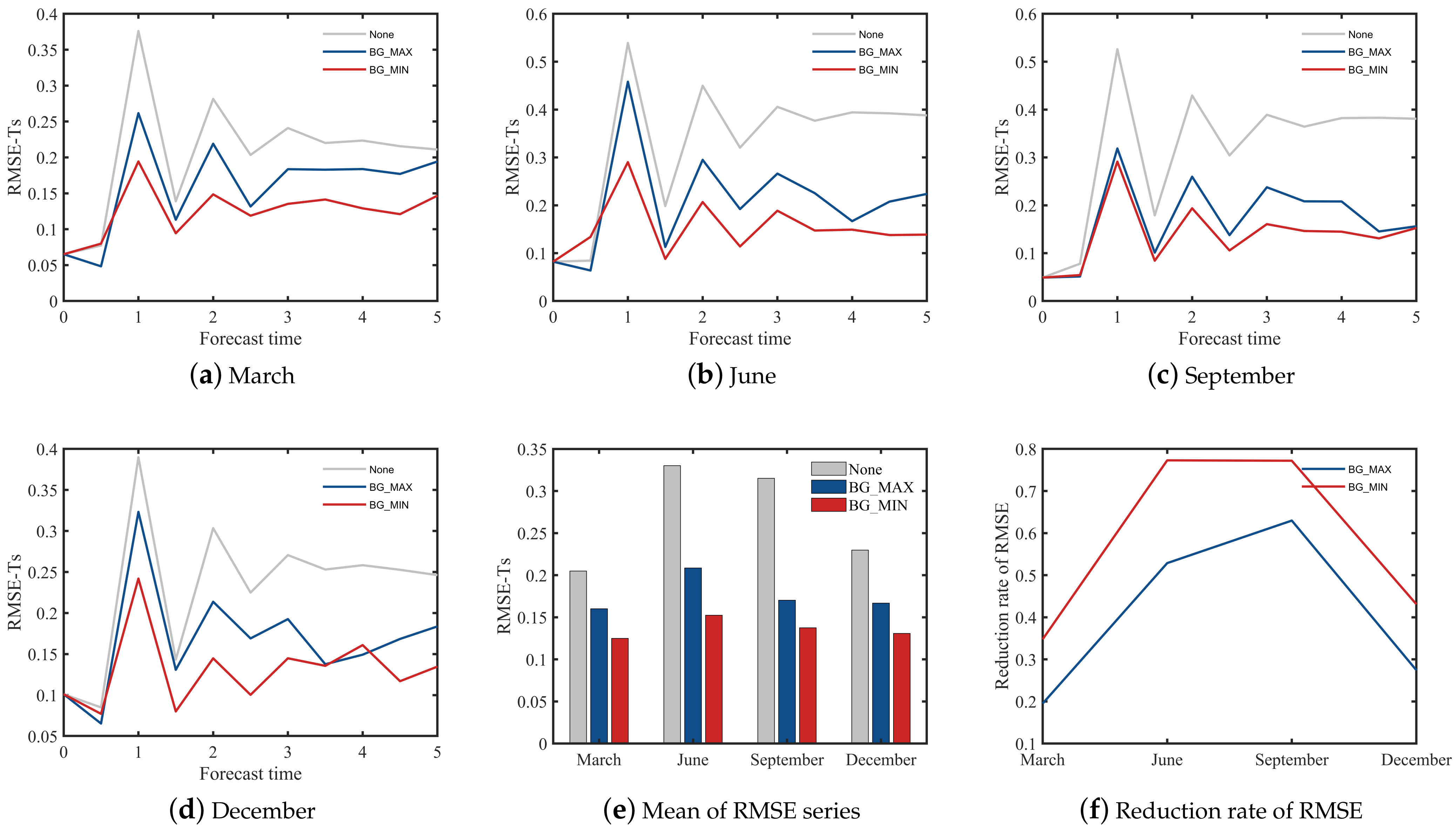
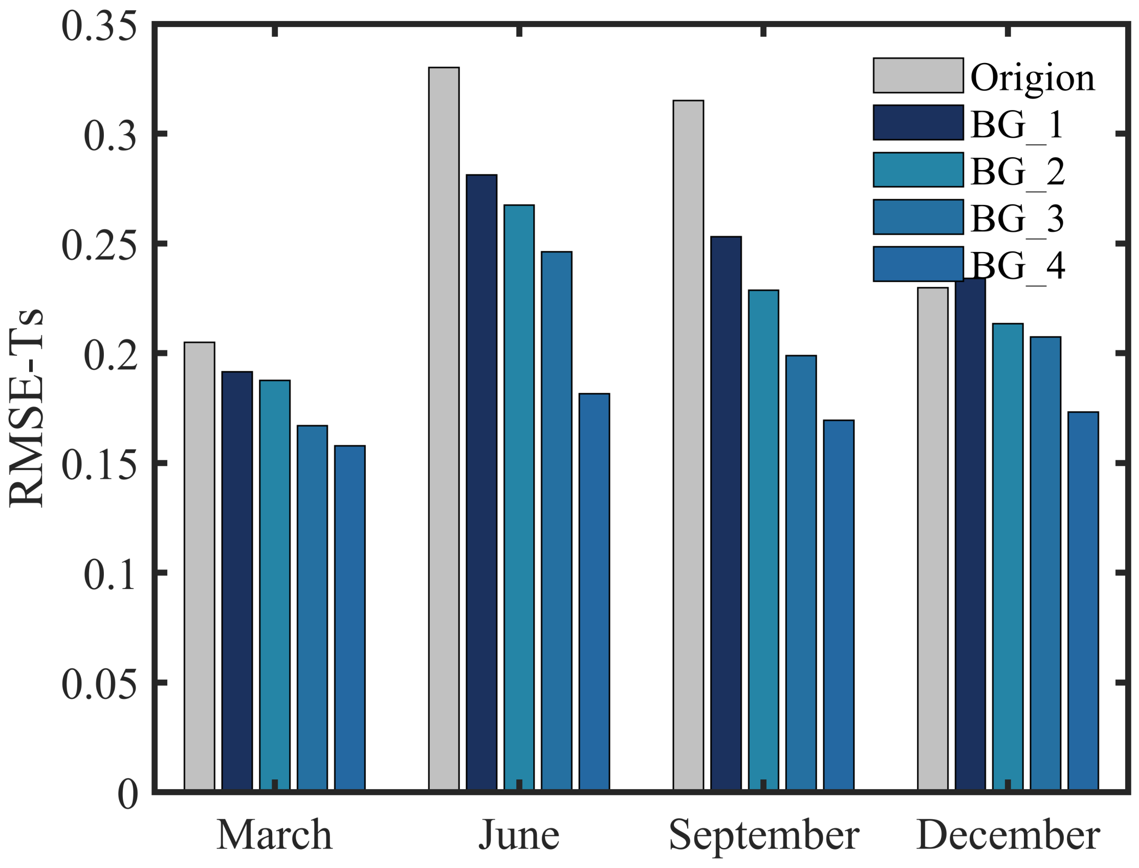
3.1. Validation of the Background Field

The construction of background field is based on a hypothesis that the temporal variability in the ocean state can reflect the sample value. It is necessary to test the hypothesis. Without loss of generality, the forecasts from 1 to 5 March, June, September, and December are used in the experiment. The four-day data are evenly distributed over different seasons of the year to eliminate the influence of seasonal factors. In the preliminary validation, two sets of observation positions with the maximum background field value (BG_MAX) and the minimum background field value (BG_MIN) are selected. These two sets of observation positions are used to make the experimental results more obvious. Samples in BG_MAX and BG_MIN are input into the “twin” experimental framework with tiny observation error (obs_err = ${10}^{-3}$). The series, mean, and reduction percent of the root mean square error (RMSE) of analysis are shown in Figure 2.

The panels (a, b, c, d) in Figure 2 clearly shows that the RMSE introduced samples in BG_MIN is less than BG_MAX in most time. Exceptions also occur when the forecast error is small enough. The reductions in RMSE with samples in BG_MIN in four months are 34.8%, 77.3%, 77.2%, and 43.1%, respectively. Compared to the reductions with samples in BG_MAX (19.5%, 52.9%, 63.0%, 27.4%), the improvement is evident. However, in practical application, the observation error is not going to be ideal. In order to be closer to the actual situation, the experiment is repeated with the observation error (obs_err = ${10}^{-5}$), and the error is greater than the mean of forecast error. The result is shown in Figure 3.

When the observation error is increased, only Figure 3b retained the characteristics consistent with the above conclusion, obviously. Compared to Figure 2a,c,d and Figure 3a,c,d show that observation error has great influence on the series of RMSE, and the case even appears that observation information leads the analysis to be worse. Therefore, it is difficult to extract information from series under the condition of big observation error. However, the mean of the RMSE series still shows the regularity. From Figure 3e, the reductions in the RMSE with the samples in BG_MIN are larger than with the samples in BG_MAX. Notice that the result in December are not as obvious as the other months, and the reduction percent is only 0.4% in BG_MIN relative to BG_MAX. Because the forecast error is small enough, there is limited room for improvement.

After the preliminary conclusion is obtained, the effectiveness of the background field will be further proven by the K-means algorithm. Because the correspondence between background field and sampling value is not clear, the test is only for a rough zone partition. The experimental area is divided into four zones by the K-means algorithm. The category and clustering centers of background fields in four seasons are shown in

Table 3. Multi-layer nested process of coupled model.

Months	Category	Centers
March	BG_1	0.664387
	BG_2	0.426747
	BG_3	0.266542
	BG_4	0.126797
June	BG_1	0.667943
	BG_2	0.477465
	BG_3	0.343627
	BG_4	0.150293
September	BG_1	0.624139
	BG_2	0.432476
	BG_3	0.293865
	BG_4	0.114702
December	Var_1	0.711194
	BG_2	0.478621
	BG_3	0.298754
	BG_4	0.117448

.

In each category, 20 points are selected as sampling points. The observation error is defined as obs_err = ${10}^{-0.5}$. Experimental results are shown in Figure 4.

The four groups of experiments had consistent results. In June and September, the mean of the RMSE series had an obvious downward trend, as the background value of the sampling region decreases. In March and December, this trend has also been shown, but the forecast has limited room for improvement and some out-of-trend values may appear, such as BG_2 in December. After the above experiment, the conclusion is drawn that the temporal variability in the forecast is positively correlated to sampling value to a certain extent.

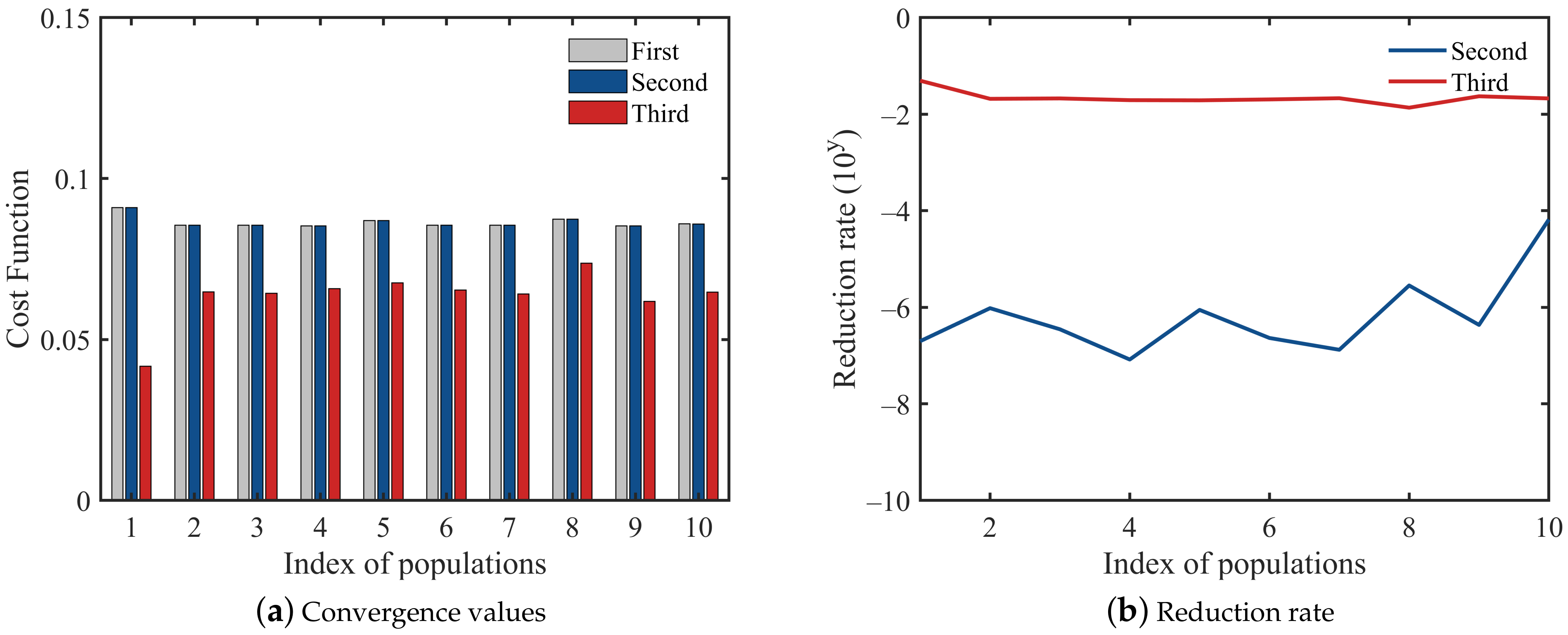
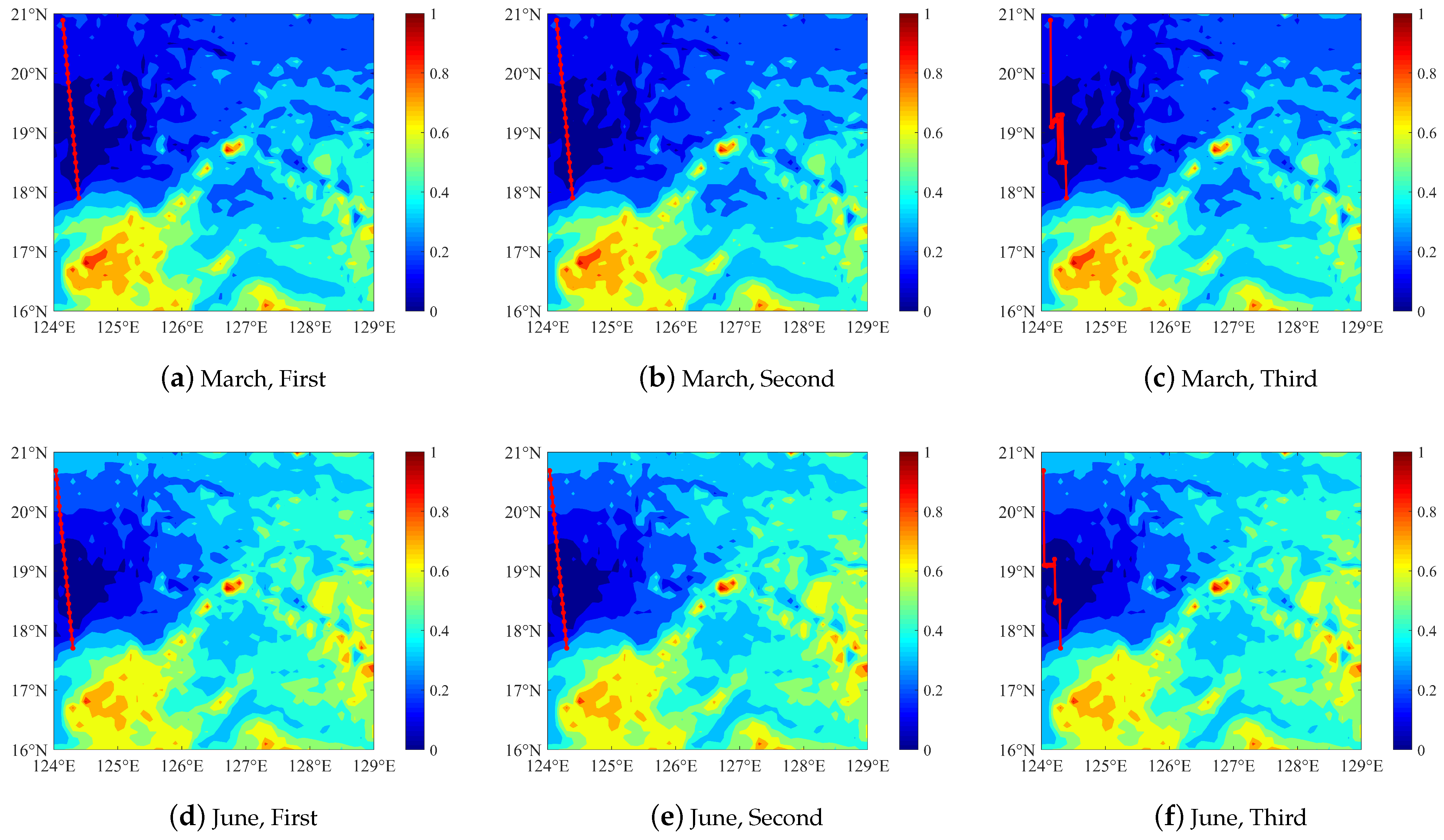
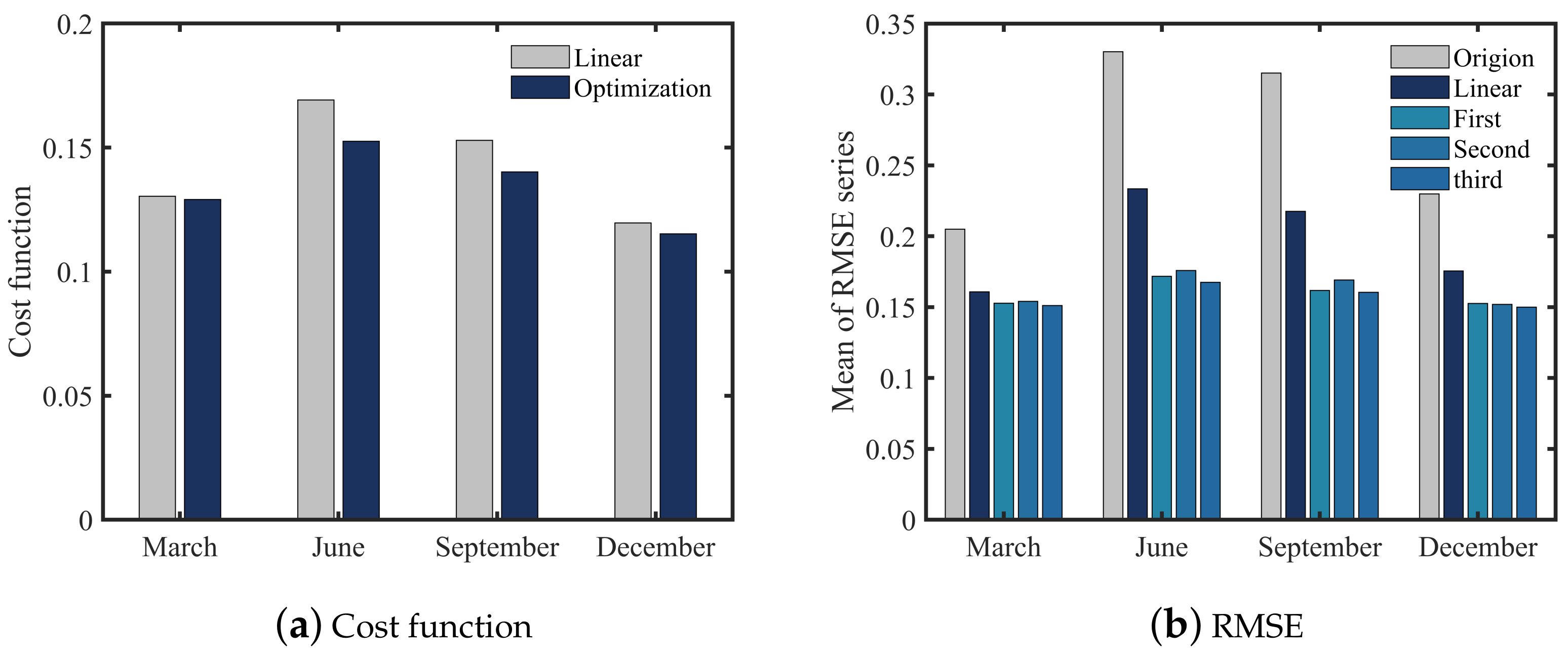
3.2. Three-Level Optimization under the Simple Cost Function

The global optimal solution calculated by BBPSO has inevitable random errors when dealing with high dimension, multi-peak, and multi-constraints. To make the result closer to ideal solution, multi-population strategies are used. Multi-population strategies are equivalent to multiple independent repetition experiments. The result obtained by multiple populations is closer to the ideal solution. Assuming that data assimilation processes were completed $n_{da}$ times, the number of sampling positions shall be an integer multiple of $n_{da}$, i.e., ($N=c_n{n}_{da},c_n\in N^{+}$). Considering the influence of path length and model resolution, to avoid repeated observation, we take $\sqrt{2}N\le r$ as a constraint. The number of sampling positions is selected as 20. The optimization process of the algorithm is shown in Figure 5. Figure 5a–c correspond to the optimization process of 10 populations in the high degree of freedom, medium degree of freedom, and low degree of freedom. The line segments of different colors in the figure represent 10 independent populations. Figure 5d represents the iterative process of the optimal solution in the three-level optimization.

In Figure 5a, initial values of the cost function are about 0.2, and few populations reached 0.25. This value is the global optimal solution searched by the whole population at the beginning. Therefore, it is slightly less than the random choice. After the first optimization, the value of the cost function all drop below 0.1, and $x_{s1},x_{s2}$, and ${\theta }_{x_{s1},x_{s2}}^{{*}^{\prime }}$ have been obtained, which leads to the small initial value of the second optimization. The second optimization is essentially the re-optimization of the first optimization. Hence, the value of cost function does not decrease much. In the first and second optimization, because the particle dimension is less. The curve converges quickly. The curves of 10 populations converge within 100 generations. However, in the third optimization, the curve does not converge until the 200th generation. In the third optimization, the convergence value of one population reached 0.04, which is significantly different from the other nine populations. The difference is caused by the slight difference in the previous two optimizations. The three-level optimization process of the population finding out the optimal solution is shown in Figure 5d. The blue, red and yellow lines represent the first, second and third optimization process respectively. In the first two optimizations, the optimal solution is used as the initial condition for the next optimization.

Convergence values of three-level optimization are compared as Figure 6. Since the results are similar in all four months, only the results in March are presented.

From Figure 6a, the population that finds the optimal value in previous two optimizations may not find the optimal value in the third optimization. The results after the previous two optimizations can be used as a heuristic factor (similar to A*) of the third optimization. Compared to previous optimization, the second optimization is improved about ${10}^{-8}$ to ${10}^{-4}$. It shows that the ensemble estimation method used in the first optimization is effective. The second optimization has less room for improvement. Compared to the second optimization, the third optimization has obvious improvement. Because the observation positions have changed significantly, the minimum after three optimizations is between 0.04 and 0.05. And the improved effect on the previous optimization is between ${10}^{-2}$ and ${10}^{-1}$.

The observation scheme obtained after three optimizations is shown in Figure 7. The color bar represents the value of the background field, and the red line on background represents the observation scheme based on a single platform. Each column represents an optimization, and each row represents a month. There are commonalities in the experimental results of four different months. For the observation scheme designed with high degrees of freedom, the observation platform is placed in the northwest, which is consistent with the background field. The scheme in Figure 7b,e,h,k is basically the same as in Figure 7a,d,g,j, which drew a similar conclusion to Figure 6. In the absence of the observation platform attribute constraints, the sampling positions after the third optimization are all concentrated in the area with small a background field value. The result accords a simple cost function but does not meet the actual condition.

3.3. Improved Cost Function

In order to make the observation scheme meet the actual situation, more constraints and the voyage function are added to the simple cost function. The global cost function can be regarded as the linear combination of the local cost function after adding the constraints. The global cost function contains the following function and constraints.

1. Temperature time variability function ($f_{\sigma }$).

2. Voyage function ($f_L$).

The range of mobile platforms is limited. Observation positions in remote area are abandoned to sample well. $f_L$ is set to be a part of global cost function; when the voyage exceeds the maximum voyage, the scheme will be re-planned. The maximum navigation range of the mobile platforms is assumed as 1000 km, and the average speed is assumed as 4.5 knots.

3. Constraint on the uniformity of sampling points ($f_U$).

The time interval of assimilation is constant. In order to reduce speed variation during navigation, $f_U$ is introduced into the global cost function. The constraint is the standard deviation of the distance between each sampling point and the previous sampling point.

4. Constraint on distance potential between sampling points ($f_P$).

$f_P$ is used to prevent multiple sampling points selected in the same area and collisions when multiple platforms are sampling simultaneously. The $f_P$ is defined as Equation (12):

$$\begin{array}{c}\hfill f_P(R_{x_i,x_j})=\frac{1}{N_r}\sum R_{x_i,x_j}\\ \hfill N_r=num(R_{x_i,x_j}\ne 0)\\ \hfill R_{x_i,x_j}=max\{1-\frac{L_{x_i,x_j}}{L_{m}ax},0\}\\ \hfill i,j\in [1,N]\cap N^{+},i\ne j\end{array}$$

(12)

$R_{x_i,x_j}$ means the distance potential between $x_i$ and $x_j$, and $L_{x_i,x_j}$ represents the distance between $x_i$ and $x_j$. $f_P$ is the mean of the distance potentials where the distance potentials are not zero.

5. Boundary cost function (D).

D is used to prevent the observation platform from colliding with obstacles or leaving the experimental area. The common feature of the boundary and obstacle is lack of background information. As the observation platform passes through these areas, a penalty value (two orders of magnitude greater than local cost function) is added to the global cost function.

6. Global cost function (F).

The global cost function is the linear combination of local cost functions after adding the constraints, which is defined as follows:

$$F_G=W_1{f}_{\sigma }+W_2{f}_L+f_U+D_0{f}_P+D$$

(13)

where $W_1$ and $W_2$ are weights. $D_0$ is the coefficient used to ensure that $f_P$ is valid. The purpose of adaptive sampling is sampling more valuable information. Therefore, the weight of the local cost function used to evaluate the value of information should be as large as possible. In this experiment, w1 is set to 0.9.

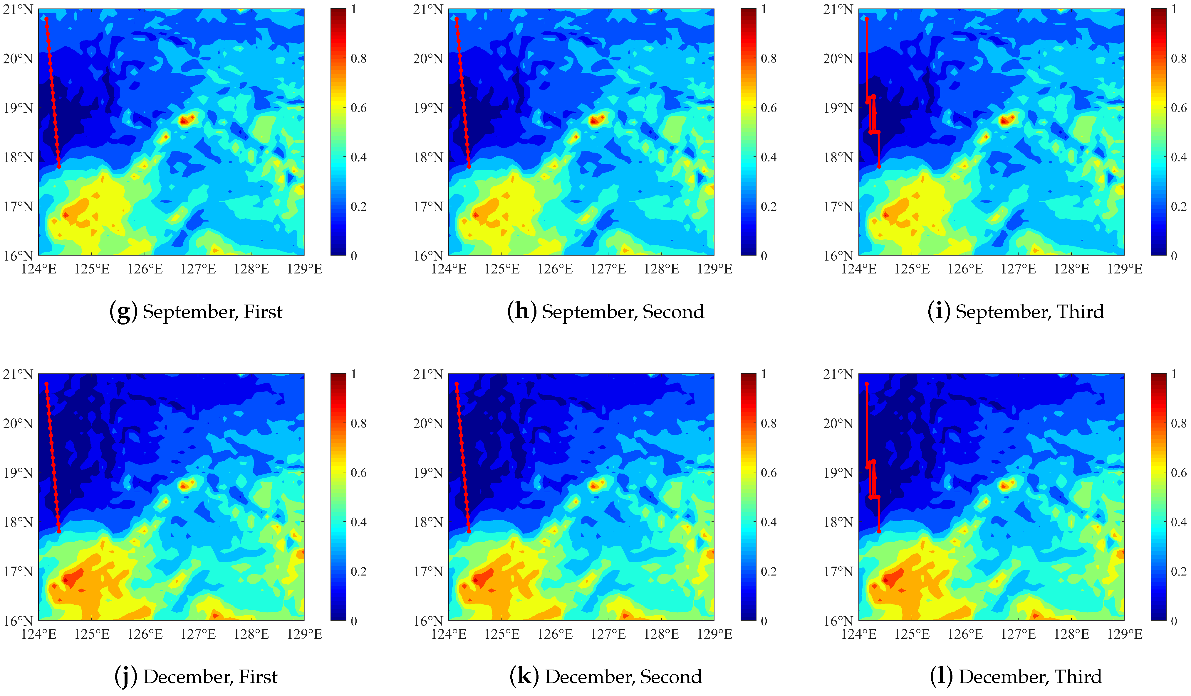
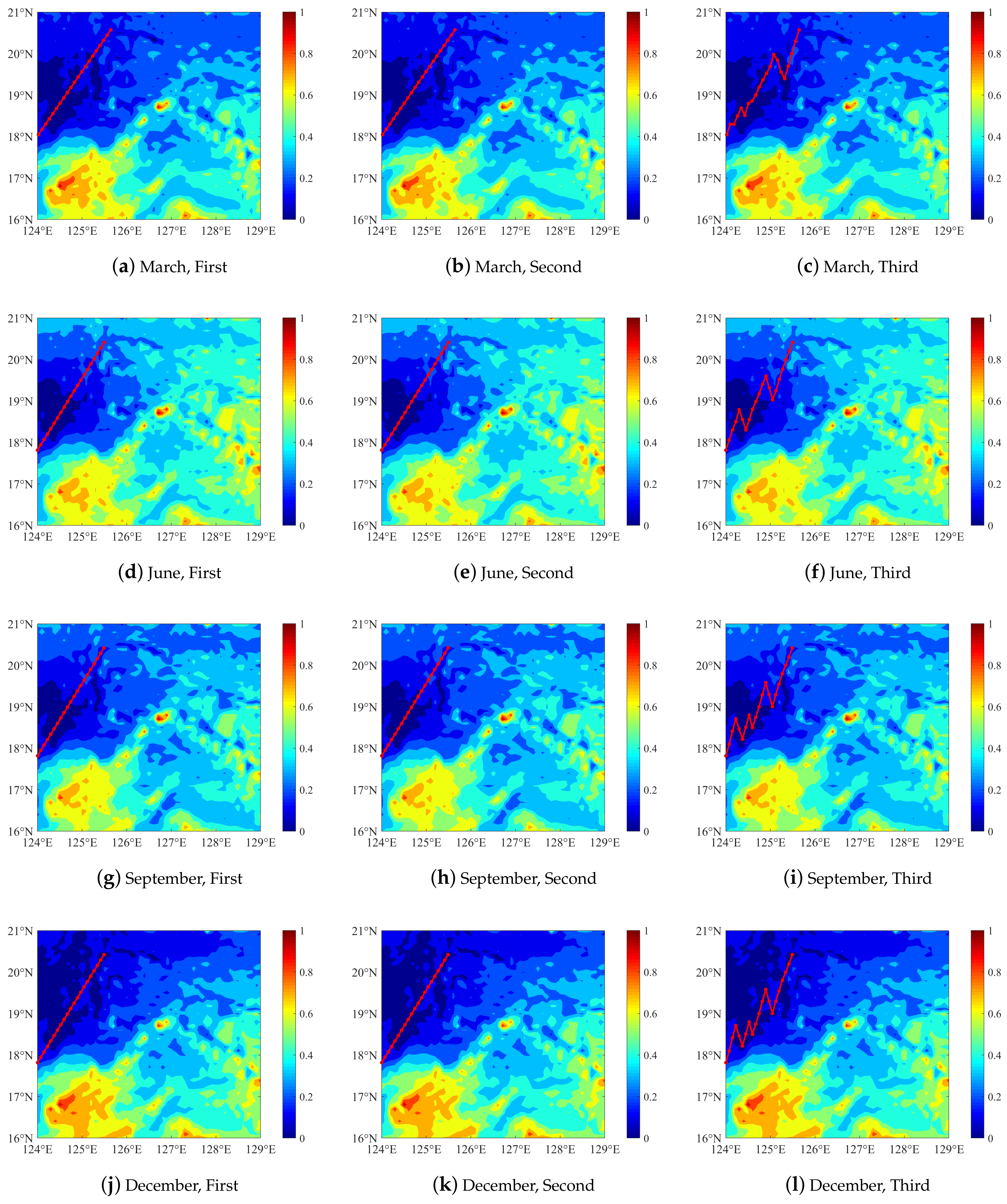
3.4. Three-Level Optimization under the Improved Cost Function

When the effective range of distance potential constraints $L_{max}\le r/N$, the best sampling scheme is the linear scheme obtained after the second optimization. First, in Euclidean space, the straight line between two points is the shortest, which led to the smallest value of $f_L$. Second, the sampling points are uniformly selected, which led to the 0 of $f_U$. Third, $L_{max}\le r/N$ means that the distance between pairs of sampling points is less than $L_{max}$, which led to $f_P$ = 0. Therefore, the linear path has obvious advantages in minimizing cost function. When the effective range of distance potential is increased to extend the spatial distribution range of sampling points, the sampling scheme designed by using the global cost function is shown in Figure 8.

The color bar represents the value of the background field, and the red line on background is the observation scheme based on a single platform. Each column represents an optimization level, and each row represents a month in Figure 8. The sampling points calculated through the third-level optimization are roughly distributed around the linear scheme. The range of observation is concentrated in the low value (blue) region, which is consistent with the intuitive experience. The scheme is similar to the usual N-type. The background fields constructed based on forecast in four months are similar, which lead the schemes to also be similar across the four months.

The third optimization can also be used for obstacle avoidance in simple terrain. To verify this feature, the midpoint of linear observation scheme is taken as the center of the obstacle. The feature of obstacle avoidance by applying the third optimization is shown in Figure 9.

The track of the mobile platform (red lines) bypasses obstacles (black circles area) in four months successfully. The third optimization takes the background into account so that there is a general plan for the direction where the mobile platform should navigate around obstacles. Notice that in the condition of simple terrain, such as in Figure 9, the initial conditions can be selected randomly. When the terrain is complex, it is necessary to combine with other path planning algorithms to provide initial conditions.

The three-level optimization method proposed can not only be used as a whole, each layer can also be applied to different situations as an independent part. The result of three-level optimization based on improved cost function is useful to find observation path through sampling sensitive location, and it also works under simple terrain conditions (with few obstacles).

4. Validation and Application of Design Methods

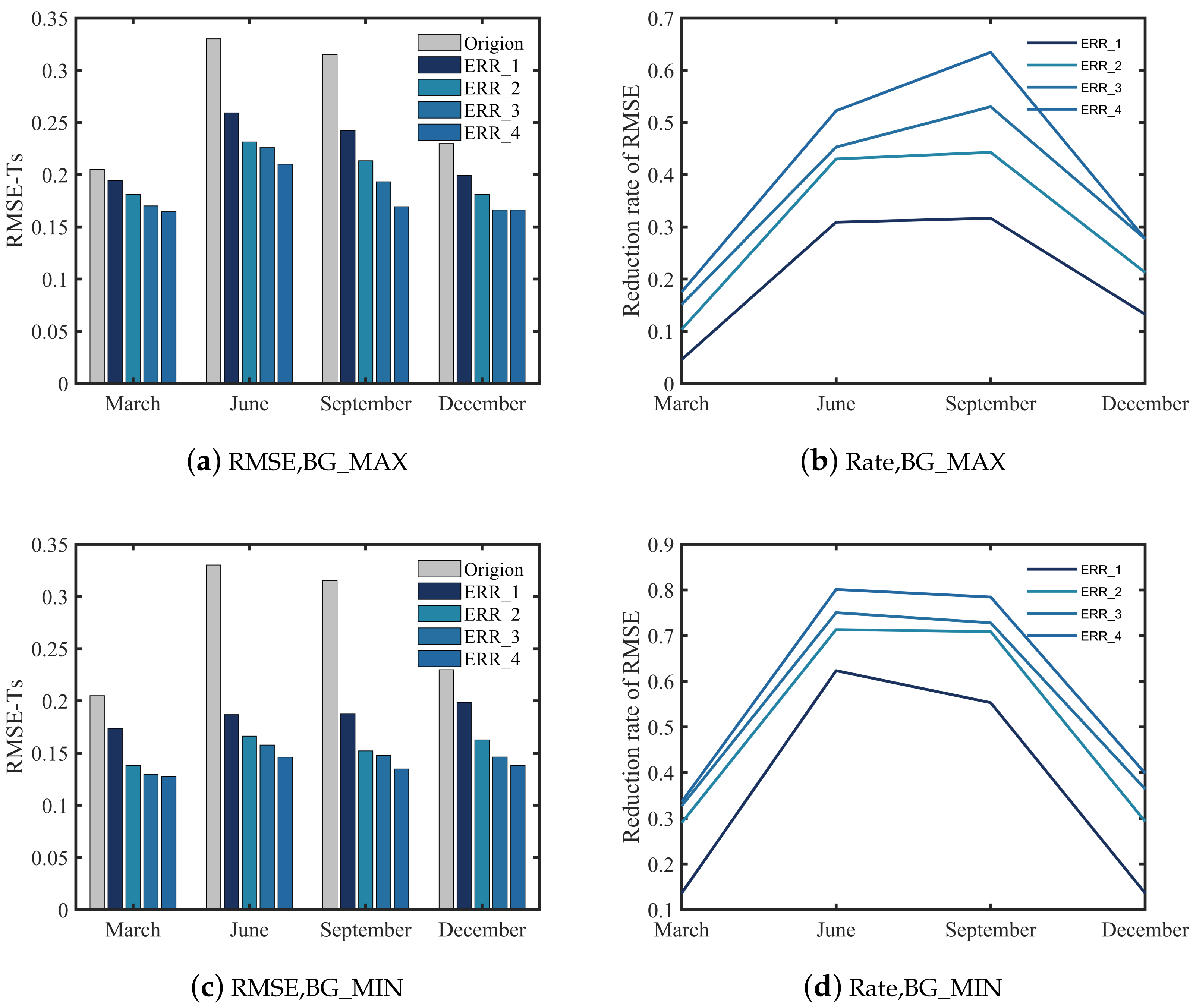
4.1. Verification of Single Platform Scheme

Results in Section 3.1 show that the observation error have accidental influence on experiment. The influence is further analyzed before twin framework used. From Figure 2, the mean of the RMSE series of forecast is between 0.2 and 0.35. In order to make the analysis better than the forecast, the observation error standard should be equal to or slightly smaller than the forecast. Meanwhile, to improve the experimental efficiency, the observation errors are selected by the experiment. Four control groups are set as $ERR\_1={10}^{-0.5}$, $ERR\_2={10}^{-1}$, $ERR\_3={10}^{-1.5}$, and $ERR\_4={10}^{-2}$. Without loss of generality, observation positions set to BG_MAX and BG_MIN are both used again in this experiment. After the sampling and data assimilation processes are simulated, the RMSE of analysis is shown in Figure 10.

Figure 10a,b are the results with samples in BG_MAX, and Figure 10c,d are the results with samples in BG_MIN. From Figure 10a,c, there is also an obvious downward trend of the mean of RMSE series as the observation error decreases. Figure 10d shows the connections between months are more concentrated with ERR_2, ERR_3, and ERR_4. It suggests that the range of change gradually diminishes, starting from ERR_2. Therefore, the value of observation error is chosen as 0.1 in follow-up experiment. Forecast system in this paper can be used for qualitative analysis of ocean environment, but there is a gap, compared to operational forecasting system. Hence, the setting of the observation error is different from the real situation.

After completing the setting of experimental errors in the twin frame, we selected five linear paths evenly in the experimental area as the control group. These are shown in Figure 11. The observation range of the control group is large enough. Meanwhile, it is consistent with the actual observation without prior information.

When single-platform sampling scheme is verified, we take the first path (from top to bottom) as control group. And the first two paths (from top to bottom) are selected as control group, when two platforms simultaneous sampling scheme is verified. This setup has an advantage that control group with more platforms included control group with fewer platforms. The influence of the number of observation platforms can be studied through the control group. The experimental results under the twin frame are shown in Figure 12.

From Figure 12, there is no obvious correspondence between the accuracy of analysis and the number of observation platforms. In March, a downward trend is roughly reflected. However, observation information sampled in the third path has a negative effect on the accuracy of analysis. A similar phenomenon occurred in June. Observation information sampled in the fifth path also has a negative effect. Figure 12 proves the observation position has a great influence on sampling and that adaptive observation is a key technology in ocean observation.

After completing the setup of the twin frame and the control group, the sampling scheme design method of the single platform is verified. The verification is divided into two steps: verification based on cost function and verification based on simulation experiment in the twin framework. Comparison results of cost function between the experimental group and control group are shown in Figure 13a. The mean of the RMSE series about the analysis obtained from different schemes are shown in Figure 13b.

From Figure 13a, for the value of the cost function, the observation scheme optimized is reduced 1.0%, 9.8%, 8.3%, and 3.7% in March, June, September, and December, respectively. The gap with the experimental group is small because the observation positions of the control group are almost all located in the small value region of the background field (blue area). From Figure 13b, in the sampling simulation experiment based on the twin frame, the sampling results after each optimization are all better than the control group. The means of the RMSE series obtained according to the optimized scheme are 0.15, 0.17, 0.16, and 0.15 in March, June, September, and December, respectively. Compared to the control group, these are reduced by 6.1%, 28.3%, 26.3%, and 14.6%, respectively. Compared to the forecast, these are reduced by 26.3%, 49.3%, 49.1%, and 34.8%, respectively. The difference in the three optimizations is less than 0.01. This phenomenon shows that the optimal observation position has the characteristics of regionalization and that the sampling effect is more dependent on the selection of protection position and recovery position of the platform. In sensitive areas, it is difficult for local adjustment of the observation points to achieve the purpose of improving the sampling effect.

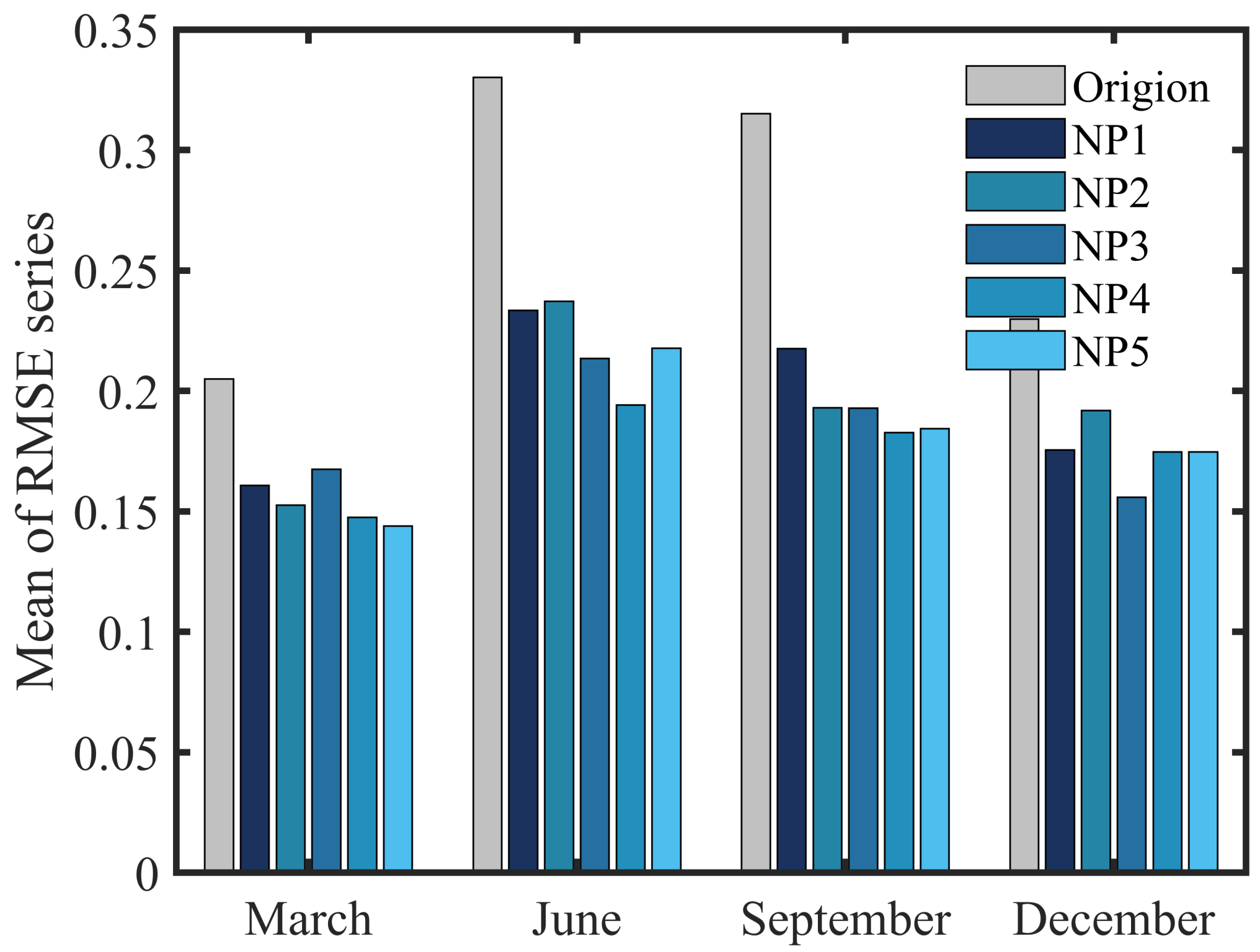
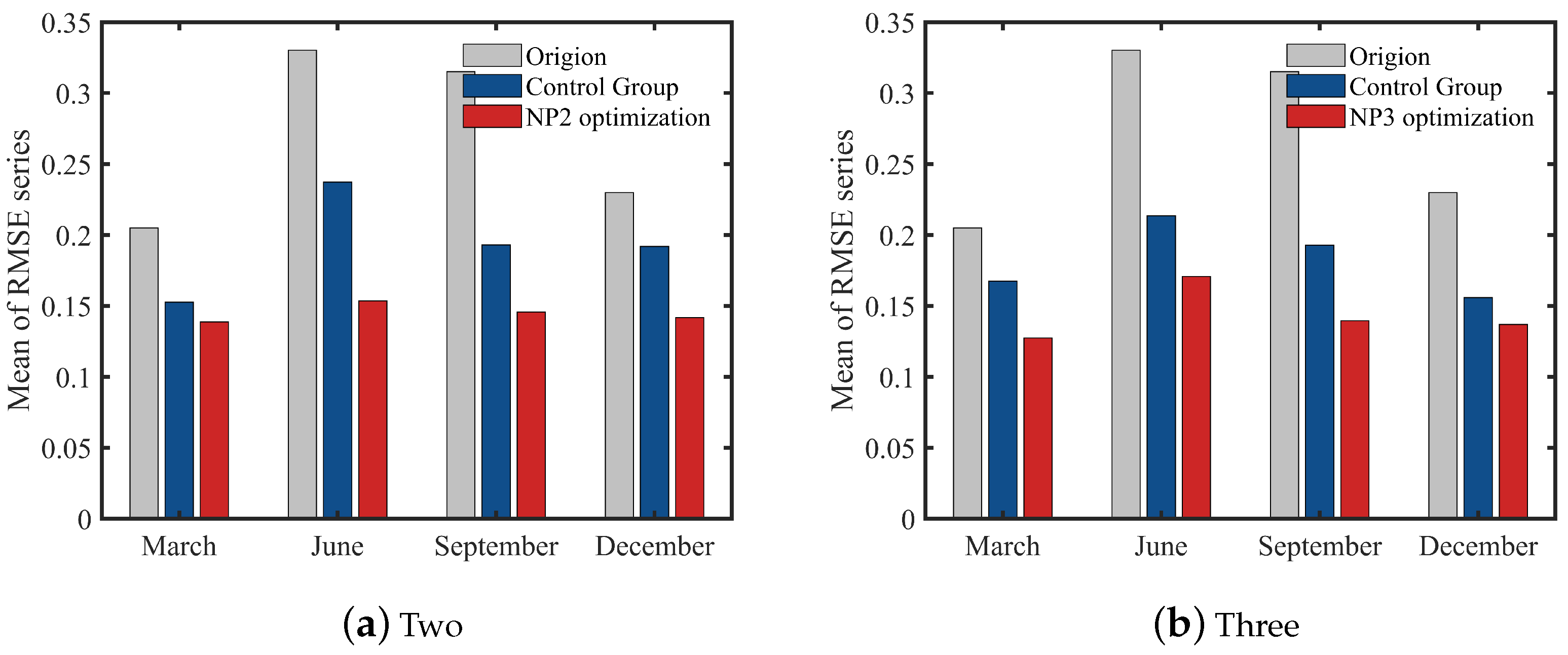
4.2. Application of Design Method in Multi-Platform Observation

The scheme design for simultaneous observation based on multiple platforms is more complicated. On the one hand, a design scheme for multiple platforms needs more computation. Meanwhile, it is also necessary to prevent collisions and repeated sampling between platforms. Some conclusions in Section 3 are helpful for this problem. Firstly, from Figure 6 it can be seen that the ensemble estimation method not only reduces the computation time but also does not reduce the accuracy obviously. Secondly, sometimes, limited by energy carrying capacity and communication conditions, the observation platform cannot change direction frequently. Thirdly, the linear scheme is optimal when deployment points and recovery points are planned and $L_{max}\le r/N$. The set of $L_{max}>r/N$ is determined for expanding the search scope, but its improvement on sampling results is limited from Figure 13b.

Two additional constraints are added to the cost function, aiming at the problem characteristics of simultaneous observation of multiple platforms.

1. Constraint on cross track.

When tracks cross, there is a risk of collision between observation platforms. This situation is avoided by imposing a penalty value into the cost function.

2. Constraint on anchor point.

In order to prevent the track of the mobile platforms from overlapping or being too close, multiple anchor points are added to the track. When the distance between anchor points is too small, penalty values are also added to the cost function.

Simultaneous sampling scheme based on 2, 3, 4, and 5 platforms in high freedom degree are shown in Figure 14. The subgraphs in the same column correspond to the same month. And the subgraphs in the same row correspond to the same number of observation platforms. From Figure 15, no matter the platform’s number and month, all platforms are concentrated in the low value region (blue or light blue areas) of the background field. A distance between the sampling paths makes the sampling range enlarged. That is what a constraint on an anchor point does.

According to the scheme above, the sampling process is simulated in a twin framework. The means of the RMSE series of analysis are compared to the control group in Figure 15. Figure 15a–d describe the improvement of the forecast by sampling based on two platforms, three platforms, four platforms, and five platforms. Compared to the control groups (blue bar), the optimized scheme (red bar) has a certain improvement in the different months and the different number of platforms. For example, in Figure 15a, the means of the RMSE series of optimized analysis are 0.14, 0.15, 0.15, and 0.14. Compared to the control group, they decrease by about 9.1%, 35.3%, 24.6%, and 26.1% in March, June, September, and December, respectively. Compared to the original forecast, it decreased by about 32.3%, 53.5%, 53.8%, and 38.3%. The same results are found on a different number of platforms. When designing a multi-platform simultaneous observation scheme, the conclusion of a single platform hierarchical optimization is applied. Compared with the control group under the condition of a high degree of freedom, the observation effect of the adaptive observation scheme is improved in different months and different numbers of platforms.

5. Summary and Discussions

We designed a systematic process for adaptive sampling on mobile assets. Through the three-layer optimization framework, multiple sampling scenarios are connected in series. Factors affecting sampling are studied in a twin experimental frame. Finally, the conclusions of these studies are applied to the situation of simultaneous observations of multiple mobile platforms.

We first constructed the background field according to the time variability of bins. Due to the probability of sampling process and the complexity of internal dynamics, the background field and sampling error cannot correspond completely. In order to solve this problem, we use a k-means algorithm to classify the background field region and test it through comparison between categories. The series of RMSE are more easily affected by observation error. Therefore, we set the mean of the series as the criterion to evaluate the analysis. Then, for multi-case transformation, we propose a hierarchical optimization framework. BBPSO is used for the optimization problem. In the high degree of freedom situation, we use ensemble estimation to speed up the calculation. Experiments show that this method is effective in low dimensional problems. In the low degree of freedom situation, we improved the cost function by adding sampling constraints. The result is similar to the common N-type sampling path. The method under constraints has a simple obstacle avoidance ability. The sampling scheme is simulated in the twin framework. We find that in a certain area, especially when the difference of the background field is small, local adjustment of the sampling position does not affect the sampling effect. Therefore, in the follow-up experiment, we pay more attention to the location of deployment and recovery. During the experiment of simultaneous multi-platform observation, we obtain the conclusion that under the twin framework used in this paper, the number of assets has little influence on the sampling effect. Finally, the optimized multi-platform scheme is simulated in the twin framework, and the result is superior to the control scheme in different times and numbers of platforms.

However, the experiment is based on the multi-layer nested coupling model, whose simulation of the real situation is limited. The conclusion needs to be verified further by a more accurate model. The hierarchical optimization framework proposed in this paper has some limitations, resulting in the separation between the layout point, recovery point, and key nodes. As a result, sampling schemes tend to search along or around a straight line. Subsequently, we will complete the integrated design between the starting points, ending points, and observation nodes by improving the cost function. In addition, the method can be combined with a path planning algorithm to realize obstacle avoidance in complex terrain environments. Moreover, there are many methods to construct an adaptive sampling background field, which can provide effective reference information for sampling. How to combine these messages and obtain a background field that can better reflect the sampling value also needs to be further studied.

References

1. Liu, Y.; Wang, M.; Su, Z.; Luo, J.; Xie, S.; Peng, Y.; Pu, H.; Xie, J.; Zhou, R. Multi-AUVs Cooperative Target Search Based on Autonomous Cooperative Search Learning Algorithm. J. Mar. Sci. Eng. 2020, 8, 843. [Google Scholar] [CrossRef]
2. Li, X.; Xu, X.; Yan, L.; Zhao, H.; Zhang, T. Energy-Efficient Data Collection Using Autonomous Underwater Glider: A Reinforcement Learning Formulation. Sensors 2020, 20, 3758. [Google Scholar] [CrossRef] [PubMed]
3. Feng, H.; Yu, J.; Huang, Y.; Qiao, J.; Wang, Z.; Xie, Z.; Liu, K. Adaptive coverage sampling of thermocline with an autonomous underwater vehicle. Ocean. Eng. 2021, 233, 109151. [Google Scholar] [CrossRef]
4. Hu, Y.; Wang, D.; Li, J.; Wang, Y.; Shen, H. Adaptive Environmental Sampling for Underwater Vehicles Based on Ant Colony Optimization Algorithm. In Proceedings of the Global Oceans 2020: Singapore—US Gulf Coast, Virtual, 5–30 October 2020; IEEE: Biloxi, MS, USA, 2020; pp. 1–9. [Google Scholar] [CrossRef]
5. Klonaris, G.; Van Eeden, F.; Verbeurgt, J.; Troch, P.; Constales, D.; Poppe, H.; De Wulf, A. ROMS Based Hydrodynamic Modelling Focusing on the Belgian Part of the Southern North Sea. J. Mar. Sci. Eng. 2021, 9, 58. [Google Scholar] [CrossRef]
6. Badriana, M.R.; Lee, H.S. Multimodel Ensemble Projections of Wave Climate in the Western North Pacific Using CMIP6 Marine Surface Winds. J. Mar. Sci. Eng. 2021, 9, 835. [Google Scholar] [CrossRef]
7. Heaney, K.D.; Lermusiaux, P.F.J.; Duda, T.F.; Haley, P.J. Validation of genetic algorithm-based optimal sampling for ocean data assimilation. Ocean. Dyn. 2016, 66, 1209–1229. [Google Scholar] [CrossRef] [Green Version]
8. Heaney, K.D.; Gawarkiewicz, G.; Duda, T.F.; Lermusiaux, P.F.J. Nonlinear optimization of autonomous undersea vehicle sampling strategies for oceanographic data-assimilation. J. Field Robot. 2007, 24, 437–448. [Google Scholar] [CrossRef] [Green Version]
9. Ma, K.; Liu, L.; Heidarsson, H.K.; Sukhatme, G.S. Data-driven learning and planning for environmental sampling. J. Field Robot. 2018, 35, 643–661. [Google Scholar] [CrossRef] [Green Version]
10. Xiong, C.; Lu, D.; Zeng, Z.; Lian, L.; Yu, C. Path Planning of Multiple Unmanned Marine Vehicles for Adaptive Ocean Sampling Using Elite Group-Based Evolutionary Algorithms. J. Intell. Robot. Syst. 2020, 99, 875–889. [Google Scholar] [CrossRef]
11. Zhang, L.; Mou, J.; Chen, P.; Li, M. Path Planning for Autonomous Ships: A Hybrid Approach Based on Improved APF and Modified VO Methods. J. Mar. Sci. Eng. 2021, 9, 761. [Google Scholar] [CrossRef]
12. Zhang, Z.; Wu, D.; Gu, J.; Li, F. A Path-Planning Strategy for Unmanned Surface Vehicles Based on an Adaptive Hybrid Dynamic Stepsize and Target Attractive Force-RRT Algorithm. J. Mar. Sci. Eng. 2019, 7, 132. [Google Scholar] [CrossRef] [Green Version]
13. Sun, Y.; Ran, X.; Zhang, G.; Xu, H.; Wang, X. AUV 3D Path Planning Based on the Improved Hierarchical Deep Q Network. J. Mar. Sci. Eng. 2020, 8, 145. [Google Scholar] [CrossRef] [Green Version]
14. Alvarez, A.; Mourre, B. Optimum Sampling Designs for a Glider–Mooring Observing Network. J. Atmos. Ocean. Technol. 2012, 29, 601–612. [Google Scholar] [CrossRef] [Green Version]
15. Liu, C.; Lei, Y.; Gao, F.; Zhao, M. Optimal Configuration Method of Sampling Points Based on Variability of Sea Surface Temperature. Adv. Meteorol. 2017, 2017, 5638289. [Google Scholar] [CrossRef] [Green Version]
16. Mu, M.; Duan, W.S.; Wang, B. Conditional nonlinear optimal perturbation and its applications. Nonlinear Process. Geophys. 2003, 10, 493–501. [Google Scholar] [CrossRef]
17. Zhao, S.; Li, W.; Cao, J. A User-Adaptive Algorithm for Activity Recognition Based on K-Means Clustering, Local Outlier Factor, and Multivariate Gaussian Distribution. Sensors 2018, 18, 1850. [Google Scholar] [CrossRef] [Green Version]
18. Anbalagan, B.; Karnam Anantha, S.; Arjunan, S.; Balasubramanian, V.; Murugesan, M. A Non-Invasive IR Sensor Technique to Differentiate Parkinson’s Disease from Other Neurological Disorders Using Autonomic Dysfunction as Diagnostic Criterion. Sensors 2021, 22, 266. [Google Scholar] [CrossRef]
19. Eberhart, R.; Kennedy, J. A new optimizer using particle swarm theory. In Proceedings of the MHS’95—Sixth International Symposium on Micro Machine and Human Science, Nagoya, Japan, 4–6 October 1995; IEEE: Nagoya, Japan, 1995; pp. 39–43. [Google Scholar] [CrossRef]
20. Kennedy, J. Bare bones particle swarms. In Proceedings of the 2003 IEEE Swarm Intelligence Symposium SIS’03 (Cat. No.03EX706), Indianapolis, IN, USA, 26 April 2003; IEEE: Indianapolis, IN, USA, 2003; pp. 80–87. [Google Scholar] [CrossRef]
21. Shang, W.; Xue, W.; Li, Y.; Wu, X.; Xu, Y. An Improved Underwater Electric Field-Based Target Localization Combining Subspace Scanning Algorithm And Meta-EP PSO Algorithm. J. Mar. Sci. Eng. 2020, 8, 232. [Google Scholar] [CrossRef] [Green Version]
22. Zheng, Q.; Feng, B.W.; Liu, Z.Y.; Chang, H.C. Application of Improved Particle Swarm Optimisation Algorithm in Hull form Optimisation. J. Mar. Sci. Eng. 2021, 9, 955. [Google Scholar] [CrossRef]
23. Yong, Z.; Yuan, L.; Qian, Z.; Sun, X. Multi-objective optimization of building energy performance using a particle swarm optimizer with less control parameters. J. Build. Eng. 2020, 32, 101505. [Google Scholar] [CrossRef]
24. Zhang, X.; Zhang, S.; Liu, Z.; Wu, X.; Han, G. Parameter Optimization in an Intermediate Coupled Climate Model with Biased Physics. J. Clim. 2015, 28, 1227–1247. [Google Scholar] [CrossRef]
25. Anderson, J.L. An Ensemble Adjustment Kalman Filter for Data Assimilation. Mon. Weather Rev. 2001, 129, 2884–2903. [Google Scholar] [CrossRef] [Green Version]
26. Dommenget, D.; Flöter, J. Conceptual understanding of climate change with a globally resolved energy balance model. Clim. Dyn. 2011, 37, 2143–2165. [Google Scholar] [CrossRef]
27. Wu, X.; Zhang, S.; Liu, Z.; Rosati, A.; Delworth, T.L.; Liu, Y. Impact of Geographic-Dependent Parameter Optimization on Climate Estimation and Prediction: Simulation with an Intermediate Coupled Model. Mon. Weather Rev. 2012, 140, 3956–3971. [Google Scholar] [CrossRef]
28. Thompson, S.L.; Warren, S.G. Parameterization of Outgoing Infrared Radiation Derived from Detailed Radiative Calculations. J. Atmos. Sci. 1982, 39, 2667–2680. [Google Scholar] [CrossRef] [Green Version]
29. Zhao, Y.; Deng, X.; Zhang, S.; Liu, Z.; Liu, C. Sensitivity determined simultaneous estimation of multiple parameters in coupled models: Part I—Based on single model component sensitivities. Clim. Dyn. 2019, 53, 5349–5373. [Google Scholar] [CrossRef]
30. Zhang, S.; Harrison, M.J.; Rosati, A.; Wittenberg, A. System Design and Evaluation of Coupled Ensemble Data Assimilation for Global Oceanic Climate Studies. Mon. Weather Rev. 2007, 135, 3541–3564. [Google Scholar] [CrossRef] [Green Version]
31. Zhang, S. A Study of Impacts of Coupled Model Initial Shocks and State–Parameter Optimization on Climate Predictions Using a Simple Pycnocline Prediction Model. J. Clim. 2011, 24, 6210–6226. [Google Scholar] [CrossRef] [Green Version]
32. Zhang, S.; Liu, Z.; Rosati, A.; Delworth, T. A study of enhancive parameter correction with coupled data assimilation for climate estimation and prediction using a simple coupled model. Tellus A Dyn. Meteorol. Oceanogr. 2012, 64, 10963. [Google Scholar] [CrossRef] [Green Version]
33. Wu, X.; Li, W.; Han, G.; Zhang, L.; Shao, C.; Sun, C.; Xuan, L. An Adaptive Compensatory Approach of the Fixed Localization in the EnKF. Mon. Weather Rev. 2015, 143, 4714–4735. [Google Scholar] [CrossRef]
34. Gaspari, G.; Cohn, S.E. Construction of correlation functions in two and three dimensions. Q. J. R. Meteorol. Soc. 1999, 125, 723–757. [Google Scholar] [CrossRef]
35. Pan, F.; Hu, X.; Eberhart, R.; Chen, Y. An analysis of Bare Bones Particle Swarm. In Proceedings of the 2008 IEEE Swarm Intelligence Symposium, St. Louis, MO, USA, 21–23 September 2008; IEEE: St. Louis, MO, USA, 2008; pp. 1–5. [Google Scholar] [CrossRef]
36. Shi, Y.; Eberhart, R.C. Parameter selection in particle swarm optimization. In Evolutionary Programming VII; Lecture Notes in Computer Science Series; Goos, G., Hartmanis, J., van Leeuwen, J., Porto, V.W., Saravanan, N., Waagen, D., Eiben, A.E., Eds.; Springer: Berlin/Heidelberg, Germany, 1998; Volume 1447, pp. 591–600. [Google Scholar] [CrossRef]
37. Zhang, E.; Wu, Y.; Chen, Q. A practical approach for solving multi-objective reliability redundancy allocation problems using extended bare-bones particle swarm optimization. Reliab. Eng. Syst. Saf. 2014, 127, 65–76. [Google Scholar] [CrossRef]
Figure 1. The flow chart of the twin experiment framework’s setup with ICCM.
Jmse 10 00664 g001
Figure 2. Comparison of analysis accuracy after introducing samples in BG_MAX and BG_MIN with obs_err = 10 3 .
Jmse 10 00664 g002
Figure 3. Comparison of analysis accuracy after introducing samples in BG_MAX and BG_MIN with obs_err = 10 0.5 .
Jmse 10 00664 g003
Figure 4. The mean of the RMSE series analysis introduced different observation position sets in four months.
Jmse 10 00664 g004
Figure 5. Three-level optimization process based on the BBPSO algorithm.
Jmse 10 00664 g005
Figure 6. Convergence values of various populations in a three-level optimization process.
Jmse 10 00664 g006
Figure 7. Three-times optimized observation schemes in different months based on a simple cost function.
Jmse 10 00664 g007aJmse 10 00664 g007b
Figure 8. Three optimized observation schemes in different months based on improved cost function.
Jmse 10 00664 g008
Figure 9. Obstacle avoidance based on the third optimization.
Jmse 10 00664 g009
Figure 10. The mean and reduction rate of RMSE in different observation error conditions.
Jmse 10 00664 g010
Figure 11. The control group used to test the observation scheme.
Jmse 10 00664 g011
Figure 12. The influence of the number of observation platforms on the mean of RMSE series of analysis.
Jmse 10 00664 g012
Figure 13. Verification of design methods based on a single platform.
Jmse 10 00664 g013
Figure 14. Optimal sampling scheme based on 2, 3, 4, and 5 platforms in the high degree of freedom.
Jmse 10 00664 g014
Figure 15. Average RMSE and its reduction rate of analysis in the control group and the experimental group of multi-platform optimization.
Jmse 10 00664 g015aJmse 10 00664 g015b