Hydrodynamics of a Moored Permeable Vertical Cylindrical Body

Abstract

In this study, the problems of diffraction and radiation of water waves by a permeable vertical cylindrical body are formulated within the realm of the linear potential theory. The body, which is floating in constant water depth, is moored with a catenary mooring line system. The method of matched eigenfunction expansions for the prediction of the velocity potential in the fluid domain surrounding the body is applied. Furthermore, the static and dynamic characteristics of the mooring system are combined with the hydrodynamics of the body, to set up the coupled motion equations of the dynamical model, i.e., floater and mooring system, in the frequency domain. Numerical results obtained through the developed solution are presented. The results revealed that porosity plays a key role in reducing/controlling the exciting wave loads. As far as the mooring system is concerned, its quasi-static and dynamic characteristics, by employing several motion directions on the fairlead in accordance to varying environmental conditions, are examined, highlighting their effect on the body’s motions.

1. Introduction

Permeable floating structures have been widely applied by the marine sector to reduce the effect of incoming waves and to protect marine structures against the wave action, as they use their porous surface to decrease the transmission and reflection of wave heights. Hence, they become preferable to impermeable structures, due to their porosity, for applications such as harbor and shore protection [1,2,3,4]. Subsequently, several studies have followed concerning porous breakwaters and their capability in dissipating the wave energy, while minimizing the environmental impact [5,6,7,8,9,10,11].

Permeable floating structures are also related to aquaculture, which is gradually replacing ocean fishing. The shrinking availability of coastal sites, as well as the increased environmental impact of aquaculture, is forcing the latter into offshore areas, where the main challenge is to build a structure capable of withstanding the offshore severe environmental conditions, while being financially competitive with near-shore concepts. Cage farming has been practiced at an early phase for hundreds of years, initially in fresh water and later in seawater, whereas the development of modern cage systems has taken place in the last 30 years. Kawakami [12] was the first to evaluate the resistance of fish nets to currents using a simple analytical formula. Aarsnes et al. [13] calculated the current forces on cage systems and the deformation of nets on the basis of net-panel discretization with line finite elements in the plane of symmetry. Herein, an empirical formula for the drag coefficient of plane nets in a steady current was established. Continually, in [14], the stability and maneuverability problems of fishing gear were examined through the development of a dynamic study on submerged flexible reticulated surfaces. A multi-domain boundary element method based on Darcy’s fine pore model for the determination of the wave interaction with a horizontal porous flexible membrane was presented in [15]. Additionally, in [16] the scattering problem of a flexible fishnet, modeled as a porous, freely flexible, barrier displaced solely by hydrodynamic force and deformed similarly to a catenary, was studied. A nonlinear finite element method simulating the tension variation of a fishing net under a uniform current was presented in [17], whereas, in [18], a numerical calculation method for simulating the three-dimensional dynamic behavior of fishing nets was developed. Here, the fishing nets were modeled as a group of lumped point masses interconnected with weightless springs. In [19], a numerical model for the determination of the flow field around a 3D porous structure was presented. The model also calculated the responses of the structure taking into consideration the fluid velocity reduction due to the net. Bao et al. [20] applied a complicated dispersion equation for the evaluation of the eigenvalues of the fluid domain inside a semi-submerged porous circular cylinder. They derived an additional damping term created by the porosity.

In the recent decade, a wide range of studies on modeling the hydrodynamic problem of wave interaction with fish cages were presented, and several computational methods were developed. Indicatively, Faltinsen [21] presented a slender-body theory to simulate the wave effects on a floating fish cage with circular collar in the framework of potential flow theory without, however, considering current effects. Continually, in [22], a numerical model was developed to calculate viscous wave and current loads on aquaculture nets. Here, the net shape was determined by solving a time-stepping procedure which evaluates the unknown tensions at each timestep. The model was further developed in [23,24] to consider the induced wave and current mooring loads on a net cage. Furthermore, a cubic-shaped, elastic, fish cage was examined in [25] validating its mooring characteristics and behavior with experimental results. In [26,27], a hydroelastic analysis of surface gravity waves with floating flexible cage systems was presented considering the deflection of the porous and flexible structure, whereas, in [28], a semi-analytical model was developed describing the wave field around a submerged cylindrical fish net cage. Herein, the theory was based on linear approximation; hence, nonlinearities due to wave action or quadratic porous flow models were omitted. In addition, the wave–current effect on a moored flexible fish cage was studied in [29] through a semi-analytical model in the realm of the linearized wave theory, which was validated with numerical finite element model results. Recently, a semi-analytical model was proposed for wave interactions with a submerged flexible net cage governed by the membrane vibration equation [30].

Supplementary to aquaculture applications, permeable structures, considered as rigid bodies, were also examined as means of reducing/controlling the exciting wave loads. Specifically, in [31], a theoretical formulation was presented dealing with the wave interactions with arrays of bottom-seated, surface-piercing, circular cylinders. It was concluded that porosity significantly reduces the hydrodynamic loading, as well as the associated wave run up. The theoretical formulation was further developed in [32] to account for a freely floating circular cylinder, solving the corresponding radiation problem and concluding that the size of the porous region affects the hydrodynamic coefficients of the permeable body. In [33], the wave excitation forces on an array of freely floating, porous, circular cylinders were determined for various porous coefficients. In addition, a theoretical model, also validated experimentally, was developed in [34] to investigate the wave interactions with a truncated porous cylinder. Herein, the phenomenon of the sloshing mode inside the porous structure was observed. An array of porous circular cylinders with impermeable bottom, supplemented by horizontal, porous plates inside the bodies, was theoretically and experimentally examined in [35]. Furthermore, in [36], a 3D numerical model was developed describing the wave interactions with circular cylinders featuring a partially porous surface, leading to an optimal ratio of the porous portion to the impermeable portion, which minimizes the wave hydrodynamic impact. Furthermore, in [37,38], the effect of linear and quadratic resistance laws on porous bodies of arbitrary shape was examined. A porous bottom-seated vertical cylinder placed in front of a rigid vertical wall was studied in [39], in which a linear potential theory was assumed. It was concluded that the amplified wave effects due to the presence of the breakwater can be apparently reduced due to the presence of the porous cylinder. Recently, a CFD method was developed and experimentally validated in [40] concerning bottom-fixed porous cylinders. The method was compared with a boundary element model, applying a quadratic pressure drop condition, concluding that both methods can accurately replicate wave forces on porous cylinders.

The motivation of the present work is to evaluate the hydrodynamics of a moored, permeable body in waves on the basis of linear potential theory. The primary purpose of introducing this type of bodies is to dissipate the wave energy, effectively reducing the transmitted and reflected wave heights. Furthermore, permeable bodies are also related to aquaculture cages, the performance of which, in waves and currents, is strongly dependent on the mooring characteristics of the cage system. Therefore, in the present analysis, the problems of diffraction and radiation around a permeable vertical cylindrical body moored with a catenary mooring line system are formulated. The characteristics of the mooring system are combined with the hydrodynamics of the body, to set up the coupled motion equations of the dynamical model, i.e., floater and mooring system, in the frequency domain.

The organization of this paper is as follows: Section 2 formulates the solution of the corresponding semi-analytical diffraction and radiation problems. In Section 3, the coupled motion equations are formulated, whereas Section 4 is dedicated to the results and discussion. Lastly, the conclusions are presented in Section 5.

2. Material and Methods

2.1. Hydrodynamic Formulation

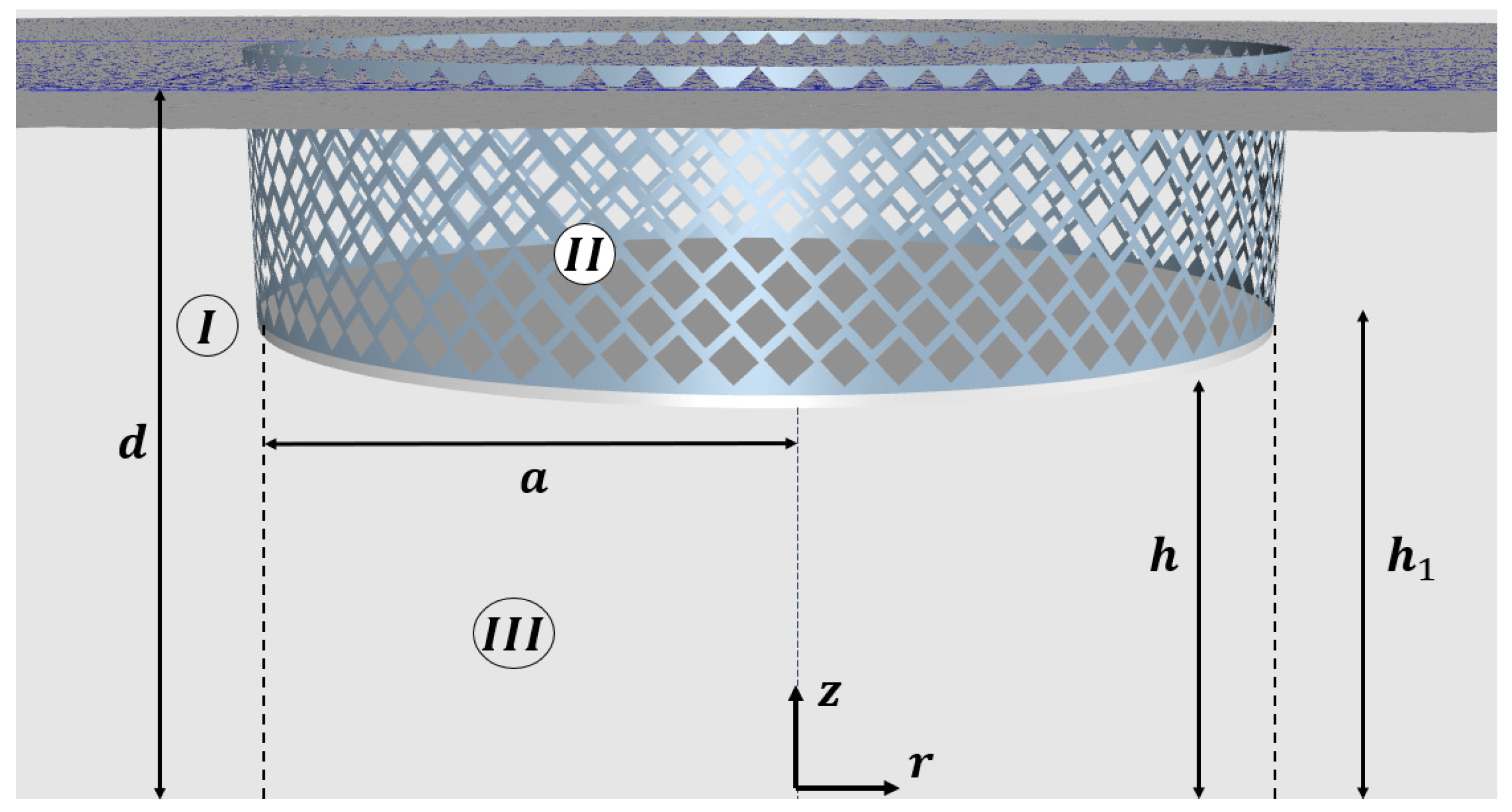
The examined vertical cylindrical body is assumed to consist of a thin impermeable bottom and a permeable sidewall of radius $\alpha$. The distance of the permeable surface bottom to the seabed is signified as $h_1$, whereas the distance of the bottom of the structure to the seabed is signified as $h$. The water depth is set to be constant, i.e., $d$, as shown in Figure 1. The permeable body is exposed to the action of regular linear waves of amplitude $H/2$, angular frequency $\omega$, and wave number $k$, propagating toward the positive direction. A cylindrical coordinate system $\left(r,\theta ,z\right)$ is adopted to describe the problem. The origin is located at the seabed, coinciding with the cylinder’s vertical symmetry axis. The fluid’s and body’s motions are assumed to be small, so that linearized diffraction and radiation problems can be considered. The water domain is subdivided into three regions: (a) fluid region $I:r\ge a, 0\le z\le d$; (b) fluid region $II:0\le r\le a, h_1\le z\le d$; (c) fluid region $III:0\le r\le a, 0\le z\le h.$ Moreover, it is assumed that the fluid is inviscid and incompressible, while the flow is irrotational and can be represented in each fluid domain in terms of velocity potential, ${\Phi }^y=\mathrm{Re}\left({\phi }^y{e}^{-i\omega t}\right), y=I,II,III$.

The velocity potential ${\phi }^y\left(r,\theta ,z\right)$ can be decomposed into three terms associated with the corresponding diffraction and radiation problems. It follows that [41]

$${\phi }^y={\phi }_0+{\phi }_7^y+{\displaystyle \sum }_{j=1,3,5}{\dot{x}}_{j0}{\phi }_j^y={\phi }_D^y+{\displaystyle \sum }_{j=1,3,5}{\dot{x}}_{j0}{\phi }_j^y.$$

(1)

In Equation (1), the velocity potential of the undisturbed incident harmonic wave is denoted as ${\phi }_0$, whereas the scattered wave potential for the permeable cylinder when it is assumed restrained to the wave impact is ${\phi }_7^y, y=I,II,III$. The radiation potential resulting from the forced oscillations of the body in the $j$-th direction, $j$ = 1, 3, 5, with unit velocity amplitude is denoted as ${\phi }_j^y, y=I,II,III$. Furthermore, the body’s complex velocity amplitude in the $j$-th direction is ${\dot{x}}_{j0}$. It should be noted that the sum of the undisturbed incident harmonic wave potential with the scattered wave potential is equal to the diffraction velocity potential, i.e., ${\phi }_D^y={\phi }_0+{\phi }_7^y, y=I,II,III$.

The velocity potential ${\phi }_j^y, j=1,3,5,7;y=I,II,III$ satisfies the Laplace equation as its governing equation. In the framework of linear wave theory, ${\phi }_j^y$ satisfies a homogeneous free surface boundary condition at $z=d$ and an impermeable boundary condition at $z=0$. In addition, the radiation and scattering potentials, $j=1,3,5,7$, have to be satisfy the Sommerfeld radiation condition at the far field [42].

Since the cylinder’s sidewall is permeable, and the Reynolds numbers of the flow through the permeable surface are low, Darcy’s law can be employed [43]. It is stated that the normal flow velocity is continuous through the porous boundary and proportional to the pressure difference through the porous boundary [31]; hence, the boundary condition on the sidewall forms

$$\frac{\partial {\phi }_j^{II}}{\partial r}=n_j+ikG\left[{\phi }_j^{II}-{\phi }_j^I\right]\mathrm{on}r=a,h_1\le z\le d, j=1,3,5,D.$$

(2)

In Equation (2), $\partial /\partial r$ denotes the derivative with respect to $r$, $k$ stands for the wave number, and $n_j$ is the generalized normal vector defined as $(n_1,n_2,n_3)=\mathrm{n}; (n_4,n_5,n_6)=\mathrm{r}$ × $\mathrm{n}$. Here, $\mathrm{n}$ is the unit normal vector pointing outward, $\mathrm{r}$ is the position vector regarding the coordinate system origin, and × the cross-product symbol.

Furthermore, $G$ denotes the complex dimensionless porous effect parameter. The parameter can be composed by $G=G_{re}+i{G}_{im}$, where $G_{re}$ represents the linearized drag effect of the permeable sidewall, and $G_{im}$ is the inertial effect. Hence, for a real $G$, the resistance effects dominate over the inertia effects, whereas $G$ attains complex values when the inertia effects dominate over the resistance ones [43]. The parameter $G$ is also a measure of the sidewall porous effect, i.e., for $G=0$, the sidewall is total impermeable, whereas, as $G$ approaches infinity, i.e., $G\gg 0$, the sidewall is completely permeable to fluid (i.e., no sidewall exists) [44]. Following [34], the porous effect parameter can be connected to the opening rate $\tau$ of the sidewall material, as well as the waveslope $\epsilon =kH/2$, through Equation (3).

$$G=\frac{\left(\frac{17.8}{\epsilon }+143.2\right){\tau }^2}{2\pi \left(1+1.06\tau \right)}.$$

(3)

In Equation (3), the opening rate $\tau$ is equal to the ratio between the area of the opening holes and the total area.

Regarding the boundary conditions that have to be fulfilled by the velocity potentials ${\phi }_j^y, j=1,3,5,7;y=I,II,III$ on the cylinder’s impermeable wetted surface $S$ (i.e., $S$ is the surface of the impermeable bottom of the cylindrical body), they are formulated as follows [41]:

$$\frac{\partial {\phi }_7^I}{\partial n}=-\frac{\partial {\phi }_0}{\partial n} \mathrm{on} S,$$

(4)

$$\frac{\partial {\phi }_j^I}{\partial n}=n_j \mathrm{on} S, j=1, 3, 5.$$

(5)

The $n_j$ term in Equation (5) was defined in Equation (2).

In addition, the matching conditions at the interface between the fluid regions (see Figure 1) should be satisfied, which are given by

$${\phi }_j^I={\phi }_j^{III};r=a;0\le z\le d;j=1, 3, 5,D,$$

(6)

$$\frac{\partial {\phi }_j^I}{\partial r}=\frac{\partial {\phi }_j^{II}}{\partial r};r=a; h_1\le z\le d; j=1, 3, 5,D,$$

(7)

$$\frac{\partial {\phi }_j^I}{\partial r}=\frac{\partial {\phi }_j^{III}}{\partial r};r=a;0\le z\le h; j=1, 3, 5,D.$$

(8)

The velocity potential of the undisturbed incident wave propagating along the positive x-axis can be expressed as follows [41]:

$${\phi }_0\left(r,\theta ,z\right)=-i\omega \frac{H}{2}\frac{\cosh \left(kz\right)}{k\sinh \left(kd\right)}{\displaystyle \sum }_{m=0}^{\infty }{\epsilon }_m{i}^m{J}_m\left(kr\right)\cos \left(m\theta \right).$$

(9)

In Equation (9), ${\epsilon }_m$ denotes the Neumann’s symbol defined as ${\epsilon }_0=1$ and ${\epsilon }_m=2$ for $m>0$, and $J_m$ is the $m$-th order Bessel function of first kind.

Similar to Equation (9), the diffraction velocity potential around the permeable body can be obtained as

$${\phi }_D^y\left(r,\theta ,z\right)=-i\omega \frac{H}{2}{\displaystyle \sum }_{m=0}^{\infty }{\epsilon }_m{i}^m{\Psi }_{Dm}^y\left(r,z\right)\cos \left(m\theta \right), y=I,II,III.$$

(10)

Furthermore, the radiation potentials ${\phi }_j^y, j=1,3,5$ can be expressed as follows [41]:

$${\phi }_1^y\left(r,\theta ,z\right)={\Psi }_{11}^y\left(r,z\right)\cos \left(\theta \right), {\phi }_3^y\left(r,\theta ,z\right)={\Psi }_{30}^y\left(r,z\right), {\phi }_5^y\left(r,\theta ,z\right)={\Psi }_{51}^y\left(r,z\right)\cos \left(\theta \right).$$

(11)

The functions ${\Psi }_{Dm}^y,{\Psi }_{11}^y,{\Psi }_{30}^y,{\Psi }_{51}^y$ in Equations (10) and (11) denote the principal unknowns of the corresponding diffraction and radiation problems. Here, the superscript indicates the fluid domain, $y=I,II,III.$ Moreover, the first subscript stands for the respective boundary value problem, $D, 1, 3, 5$, and the second stands for the number of $m$ modes, which are applied in the solution procedure.

Equations (2) and (4)–(8) provide sufficient information for the treatment of the hydrodynamic problems (i.e., diffraction and radiation problems) in each fluid domain. Applying the method of separation of variables, the Laplace differential equation can be solved, and appropriate representations of the ${\Psi }_{Dm}^y,{\Psi }_{11}^y,{\Psi }_{30}^y,{\Psi }_{51}^y$ functions in each fluid domain can be established. The complete solution is obtained by applying the kinematic condition on the impermeable wetted surface, the porous boundary condition on the sidewall, and the matching relations (see Equations (6)–(8)) on the common cylindrical boundaries of the discrete fluid regions.

According to the presented formulation and similarly to [42], the following expressions for the ${\Psi }_{lm}^y, l=D,1,3,5$ terms can be derived for the description of the induced flow field around the permeable cylindrical body.

Infinite fluid region, $I$: $r\ge a, 0\le z\le d$

$$\frac{1}{{\delta }_l}{\Psi }_{lm}^I=f_{lm}^I+{\displaystyle \sum }_{i=0}^{\infty }{F}_{lm,i}^I\frac{K_m\left(a_i^{I}r\right)}{K_m\left(a_i^{I}a\right)}{Z}_i\left(z\right).$$

(12)

In Equation (12), $K_m$ is the $m$-th order modified Bessel function of second kind, whereas ${\delta }_l=d,$ for $l=D,1,3,$ and ${\delta }_5=d^2.$ The term $f_{lm}^I$ is equal to

$$f_{Dm}^I=\left(J_m\left(kr\right)-\frac{J_m\left(ka\right)}{H_m\left(ka\right)}{H}_m\left(kr\right)\right)\frac{Z_0\left(z\right)}{d{\acute{Z}}_0\left(z\right)}, f_{11}^I=f_{30}^I=f_{51}^I=0,$$

(13)

where $H_m$ is the $m$-th order Hankel function of the first kind.

In Equations (12) and (13), the terms $Z_i\left(z\right)$ are orthonormal functions in $\left[0,d\right]$ defined as follows [41]:

$$Z_0\left(z\right)=N_{0,I}^{-1/2}\cosh \left(k^{I}z\right),$$

(14)

$$Z_i\left(z\right)=N_{i,I}^{-1/2}\cos \left(a_i^{I}z\right),$$

(15)

where

$$N_{0,I}=\frac{1}{2}\left[1+\frac{\sinh \left(2k^{I}d\right)}{2k^{I}d}\right],$$

(16)

$$N_{i,I}=\frac{1}{2}\left[1+\frac{\sin \left(2a_i^{I}d\right)}{2a_i^{I}d}\right].$$

(17)

The wave number $k^I\equiv k$ is related to the wave frequency through the dispersion equation, whereas $a_i^I, i>0$ are the positive real roots of

$$\frac{{\omega }^2}{g}+a_i^I\tan \left(a_i^{I}d\right)=0,$$

(18)

where the superscript denotes the infinite fluid region $I$.

Hence, it is convenient to write $a_0^I=-ik,$ resulting in the following [45]:

$$K_0\left(-ikr\right)=\frac{\pi }{2}i{H}_0\left(kr\right).$$

(19)

Fluid region, $II$: $0\le r\le a,h_1\le z\le d$

$$\frac{1}{{\delta }_l}{\Psi }_{lm}^{II}=f_{lm}^{II}+{\displaystyle \sum }_{i=0}^{\infty }{F}_{lm,i}^{II}\frac{I_m\left(a_i^{II}r\right)}{I_m\left(a_i^{II}a\right)}{Z}_i\left(z-h_1\right).$$

(20)

In Equation (20), $I_m$ is the $m$-th order modified Bessel function of first kind. In addition, the term $Z_i\left(z-h_1\right)$ is derived as follows [41]:

$$Z_0\left(z-h_1\right)=N_{0,II}^{-1/2}\cosh \left(k^{II}\left(z-h_1\right)\right),$$

(21)

$$Z_i\left(z-h_1\right)=N_{i,II}^{-1/2}\cos \left(a_i^{II}\left(z-h_1\right)\right),$$

(22)

where:

$$N_{0,II}=\frac{1}{2}\left[1+\frac{\sinh \left(2k^{II}\left(d-h_1\right)\right)}{2k^{II}\left(d-h_1\right)}\right],$$

(23)

$$N_{i,II}=\frac{1}{2}\left[1+\frac{\sin \left(2a_i^{II}\left(d-h_1\right)\right)}{2a_i^{II}\left(d-h_1\right)}\right].$$

(24)

Furthermore, it holds that

$$f_{Dm}^{II}=f_{11}^{II}=0, f_{30}^{II}=\frac{z}{d}-1+\frac{g}{d{\omega }^2}, f_{51}^{II}=\frac{-r}{d^2}\left(\left(z-d\right)+\frac{g}{{\omega }^2}\right).$$

(25)

The terms $a_i^{II}$ are the roots of

$$\frac{{\omega }^2}{g}+a_i^{II}\tan \left(a_i^{II}\left(d-h_1\right)\right)=0,$$

(26)

with the imaginary $a_i^{II}=-i{k}^{II}$ considered as first.

Fluid region, $III$: $0\le r\le a,0\le z\le h$

$$\frac{1}{{\delta }_l}{\Psi }_{lm}^{III}=f_{lm}^{III}+{\displaystyle \sum }_{n=0}^{\infty }{\epsilon }_m{F}_{lm,n}^{III}\frac{I_m\left(\frac{n\pi }{h}r\right)}{I_m\left(\frac{n\pi }{h}a\right)}\cos \left(\frac{n\pi }{h}z\right).$$

(27)

In Equation (27), the term $f_{lm}^{III}$ is equal to

$$f_{Dm}^{III}=f_{11}^{III}=0, f_{30}^{III}=\frac{z^2-0.5r^2}{2hd}, f_{51}^{III}=\frac{-r\left(z^2-0.25r^2\right)}{2h{d}^2}.$$

(28)

The functions ${\Psi }_{lm}^y, l=D,1,3,5$ have the advantage of being expressed by simple Fourier series representations, $F_{lm,i}^I, F_{lm,i}^{II}, F_{lm,n}^{III},$ of all the types of ring regions. The system of equations for the unknown Fourier coefficients is derived by fulfilling the kinematic conditions at the vertical walls (i.e., permeable, and impermeable surfaces), as well as by the requirement for continuity of the potential and its first derivative. The formulation was described thoroughly in [42]. Hence, it is not further elaborated here.

2.2. Hydrodynamic Forces

The various hydrodynamic forces on the permeable cylindrical body are calculated by the pressure distribution given by the linearized Bernoulli’s equation. Thus, it can be written that

$$F_1=-2\pi i\rho {\omega }^{2}d\frac{H}{2}a\left[\underset{h}{\overset{d}{{\displaystyle \int }}}\frac{1}{d}{\Psi }_{D1}^I\left(a,z\right)dz-\underset{h_1}{\overset{d}{{\displaystyle \int }}}\frac{1}{d}{\Psi }_{D1}^{II}\left(a,z\right)dz\right].$$

(29)

Substituting Equations (12) and (20) into Equation (29), we get

$$\begin{gathered} \frac{F_1}{B}=-2ikd\tan \mathrm{h}\left(kd\right)[N_{0,I}^{-\frac{1}{2}}{F}_{D1,0}^I\frac{\sinh \left(kd\right)-\sinh \left(kh\right)}{ka}+{\displaystyle \sum }_{i=1}^{\infty }{N}_{i,I}^{-\frac{1}{2}}{F}_{D1,i}^I\frac{\sin \left(a_i^{I}d\right)-\sin \left(a_i^{I}h\right)}{a_i^{I}a} \\ -N_{0,II}^{-\frac{1}{2}}{F}_{D1,0}^{II}\frac{\sinh \left(k^{II}(d-h_1\right))}{k^{II}a}-{{\displaystyle \sum }}_{i=1}^{\infty }{N}_{i,II}^{-\frac{1}{2}}{F}_{D1,i}^{II}\frac{\sin \left(a_i^{II}\left(d-h_1\right)\right)}{a_i^{II}a}], \end{gathered}$$

(30)

where $B=\pi \rho g{\alpha }^2\left(\frac{H}{2}\right)$, where $\rho$ is the water density, and $g$ is the acceleration due to gravity. Similar, the vertical forces on the permeable cylindrical body are equal to the sum of the forces on the upper and lower surfaces, i.e., $0\le r\le a,$ $z=h_1$ and $z=h$, respectively. Thus,

$$F_3=2\pi \rho {\omega }^{2}d\frac{H}{2}\left[\underset{0}{\overset{a}{{\displaystyle \int }}}\frac{1}{d}{\Psi }_{D0}^{III}\left(r,h\right)rdr-\underset{0}{\overset{a}{{\displaystyle \int }}}\frac{1}{d}{\Psi }_{D0}^{II}\left(r,h_1\right)rdr\right].$$

(31)

Substituting Equations (20) and (27) into Equation (31), it is derived that

$$\begin{gathered} \frac{F_3}{B}=2kd\tan \mathrm{h}\left(kd\right)[\frac{1}{2}{F}_{D0,0}^{III}+2{\displaystyle \sum }_{n=1}^{\infty }{\left(-1\right)}^n{F}_{D0,i}^{III}\frac{1}{\frac{n\pi a}{h}}\frac{I_1\left(\frac{n\pi }{h}a\right)}{I_0\left(\frac{n\pi }{h}a\right)} \\ -N_{0,II}^{-\frac{1}{2}}{F}_{D0,0}^{II}\frac{1}{k^{II}a}\frac{J_1\left(k^{II}a\right)}{J_0\left(k^{II}a\right)}-{\displaystyle \sum }_{i=1}^{\infty }{N}_{i,II}^{-\frac{1}{2}}{F}_{D0,i}^{II}\frac{1}{a_i^{II}a}\frac{I_1\left(a_i^{II}a\right)}{I_0\left(a_i^{II}a\right)}]. \end{gathered}$$

(32)

The moment on the permeable cylindrical body about a horizontal axis at an arbitrary distance $z=e$ from the seabed can be decomposed into $M_S$ and $M_b$ terms arising from the pressure distribution on the body’s wetted surfaces (i.e., permeable and impermeable). It holds that

$$M_S=-2\pi i\rho {\omega }^{2}d\frac{H}{2}a\left[\underset{h}{\overset{d}{{\displaystyle \int }}}\frac{1}{d}{\Psi }_{D1}^I\left(a,z\right)\left(z-e\right)dz-\underset{h_1}{\overset{d}{{\displaystyle \int }}}\frac{1}{d}{\Psi }_{D1}^{II}\left(a,z\right)\left(z-e\right)dz\right],$$

(33)

$$M_b=-2\pi \rho {\omega }^{2}d\frac{H}{2}\left[\underset{0}{\overset{a}{{\displaystyle \int }}}\frac{1}{d}{\Psi }_{D1}^{III}\left(r,h\right)r^{2}dr-\underset{0}{\overset{a}{{\displaystyle \int }}}\frac{1}{d}{\Psi }_{D1}^{II}\left(r,h_1\right)r^{2}dr\right].$$

(34)

Substituting Equations (12), (20), and (27) into Equations (33) and (34), it is derived that

$$\frac{M_s}{Ba}=-2ikd\tan \mathrm{h}\left(kd\right)[N_{0,I}^{-\frac{1}{2}}{F}_{D1,0}^I{L}_0^I+{\displaystyle \sum }_{i=1}^{\infty }{N}_{i,I}^{-\frac{1}{2}}{F}_{D1,i}^I{L}_i^I-N_{0,II}^{-\frac{1}{2}}{F}_{D1,0}^{II}{L}_0^{II}-{\displaystyle \sum }_{i=1}^{\infty }{N}_{i,II}^{-\frac{1}{2}}{F}_{D1,i}^{II}{L}_i^{II}],$$

(35)

$$\begin{gathered} \frac{M_b}{Ba}=-2kdtanh\left(kd\right)[\frac{1}{4}{F}_{D1,0}^{III}+2{\displaystyle \sum }_{n=1}^{\infty }{\left(-1\right)}^n{F}_{D1,i}^{III}\frac{1}{\frac{n\pi a}{h}}\frac{I_2\left(\frac{n\pi }{h}a\right)}{I_1\left(\frac{n\pi }{h}a\right)} \\ -N_{0,II}^{-\frac{1}{2}}{F}_{D1,0}^{II}\frac{1}{k^{II}a}\frac{J_2\left(k^{II}a\right)}{J_1\left(k^{II}a\right)}-{\displaystyle \sum }_{i=1}^{\infty }{N}_{i,II}^{-\frac{1}{2}}{F}_{D1,i}^{II}\frac{1}{a_i^{II}a}\frac{I_2\left(a_i^{II}a\right)}{I_1\left(a_i^{II}a\right)}]. \end{gathered}$$

(36)

The terms $L_0^I,L_i^I,L_0^{II},L_i^{II}$ are presented in Appendix A.

Similarly, the corresponding hydrodynamic reaction forces and pitching moment, $F_{ij}$, on the permeable cylindrical body in the $i$-th direction due to its sinusoidal motion with frequency $\omega$ and unit amplitude in the $j$-th direction are equal to

$$F_{ij}=-\rho {\omega }^2\underset{S}{{\displaystyle \iint }}{\Psi }_{j0}^y\left(r,z\right)\cos \left(m\theta \right)n_{i}dS, y=I,II,III;i,j=1,3,5,$$

(37)

where $S$ stands for the wetted surface, while $n_i$ was defined in Equation (2).

In addition, Equation (37) can be written as

$$F_{ij}={\omega }^2{a}_{ij}+i\omega b_{ij}.$$

(38)

In Equation (38), $a_{ij}$ and $b_{ij}$ denote the hydrodynamic added mass and damping coefficients (both real and dependent of ω) in the $i$-th direction due to the body’s unit sinusoidal motion in the $j$-th direction.

Substituting Equations (12), (20), and (27) into Equation (37), the following relations for the nondimensional hydrodynamic coefficients can be obtained:

$$\begin{gathered} \frac{a_{11}}{\rho a^3}+i\frac{b_{11}}{\rho \omega a^3}=-\pi \frac{d}{a}[N_{0,I}^{-\frac{1}{2}}{F}_{11,0}^I\frac{\sinh \left(kd\right)-\sinh \left(kh\right)}{ka}+{\displaystyle \sum }_{i=1}^{\infty }{N}_{i,I}^{-\frac{1}{2}}{F}_{11,i}^I\frac{\sin \left(a_i^{I}d\right)-\sin \left(a_i^{I}h\right)}{a_i^{I}a} \\ -N_{0,II}^{-\frac{1}{2}}{F}_{11,0}^{II}\frac{\sinh \left(k^{II}\left(d-h_1\right)\right)}{k^{II}a}-{\displaystyle \sum }_{i=1}^{\infty }{N}_{i,II}^{-\frac{1}{2}}{F}_{11,i}^{II}\frac{\sin \left(a_i^{II}\left(d-h_1\right)\right)}{a_i^{II}a}], \end{gathered}$$

(39)

$$\begin{gathered} \frac{a_{33}}{\rho a^3}+i\frac{b_{33}}{\rho \omega a^3}=2\pi \frac{d}{a}[\left(\frac{h}{4d}-\frac{a^2}{16hd}\right)+\frac{1}{2}{F}_{30,0}^{III}+2{\displaystyle \sum }_{n=1}^{\infty }{\left(-1\right)}^n{F}_{30,i}^{III}\frac{1}{\frac{n\pi a}{h}}\frac{I_1\left(\frac{n\pi }{h}a\right)}{I_0\left(\frac{n\pi }{h}a\right)} \\ -\frac{1}{2}\left(\frac{h_1}{d}-1+\frac{g}{{\omega }^{2}d}\right)-N_{0,II}^{-\frac{1}{2}}{F}_{30,0}^{II}\frac{1}{k^{II}a}\frac{J_1\left(k^{II}a\right)}{J_0\left(k^{II}a\right)}-{\displaystyle \sum }_{i=1}^{\infty }{N}_{i,II}^{-\frac{1}{2}}{F}_{30,i}^{II}\frac{1}{a_i^{II}a}\frac{I_1\left(a_i^{II}a\right)}{I_0\left(a_i^{II}a\right)}], \end{gathered}$$

(40)

$$\frac{a_{55}}{\rho a^5}+i\frac{b_{55}}{\rho \omega a^5}=-\pi \frac{d^2}{a^2}\left(M_s+M_b\right).$$

(41)

The terms $M_s$ and $M_b$ are defined by

$$M_s=[N_{0,I}^{-\frac{1}{2}}{F}_{51,0}^I{L}_0^I+{\displaystyle \sum }_{i=1}^{\infty }{N}_{i,I}^{-\frac{1}{2}}{F}_{51,i}^I{L}_i^I-N_{0,II}^{-\frac{1}{2}}{F}_{51,0}^{II}{L}_0^{II}-{\displaystyle \sum }_{i=1}^{\infty }{N}_{i,II}^{-\frac{1}{2}}{F}_{51,i}^{II}{L}_i^{II}],$$

(42)

$$\begin{gathered} M_b=[\left(\frac{1}{8}\frac{ah}{d^2}-\frac{1}{48}\frac{a^3}{d^{2}h}\right)+\frac{1}{4}{F}_{51,0}^{III}+2{\displaystyle \sum }_{n=1}^{\infty }{\left(-1\right)}^n{F}_{51,i}^{III}\frac{1}{\frac{n\pi a}{h}}\frac{I_2\left(\frac{n\pi }{h}a\right)}{I_1\left(\frac{n\pi }{h}a\right)} \\ -\left(\frac{ag}{4d^2{\omega }^2}-\frac{a\left(d-h_1\right)}{4d^2}\right)-N_{0,II}^{-\frac{1}{2}}{F}_{51,0}^{II}\frac{1}{k^{II}a}\frac{J_2\left(k^{II}a\right)}{J_1\left(k^{II}a\right)}-{\displaystyle \sum }_{i=1}^{\infty }{N}_{i,II}^{-\frac{1}{2}}{F}_{51,i}^{II}\frac{1}{a_i^{II}a}\frac{I_2\left(a_i^{II}a\right)}{I_1\left(a_i^{II}a\right)}]. \end{gathered}$$

(43)

The terms $L_0^I,L_i^I,L_0^{II},L_i^{II}$ are presented in Appendix A.

3. Motion Equations

3.1. Mooring Line Characteristics

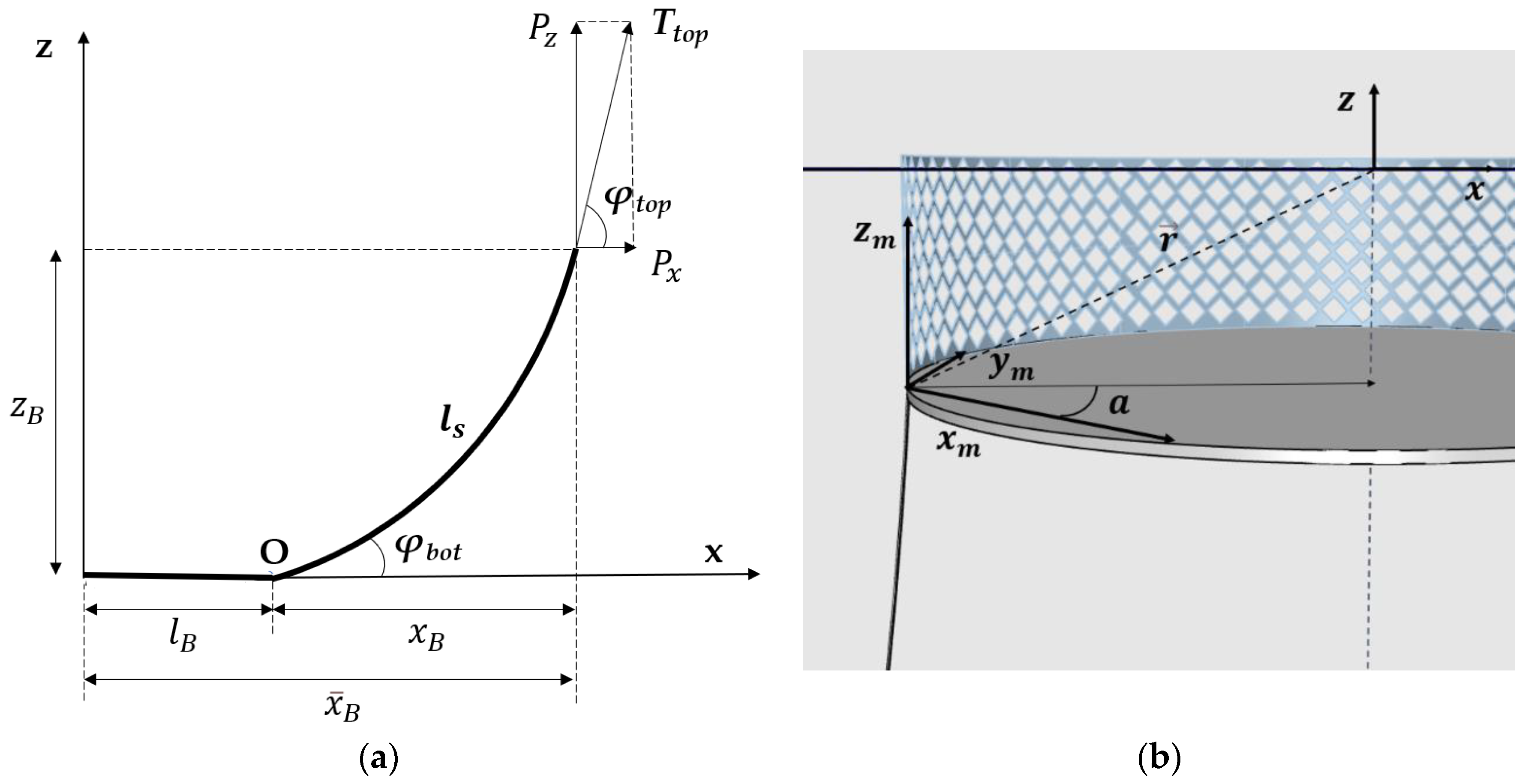
The mooring system constitutes a fundamental part for the motion response analysis of the permeable cylindrical body. In the present study, a four-point catenary mooring line system is considered. The lines are assumed as steel wires of unstretched length $L$, diameter $d_m$, and elasticity modulus $E$. The geometry of a typical mooring line in 2D is shown in Figure 2a. A global mooring cable coordinate system ($x,y,z$) is defined, located at the intersection of the body’s vertical axis of symmetry, with the undisturbed free surface, $\overrightarrow{r}$, being the position vector of the i-th line’s fairlead location with respect to the origin of the coordinate system and $a^i, i=1,2,3,4$ being the i-th line’s orientation angle in the horizontal plane (see Figure 2b). In addition, four local mooring coordinate systems ($x_m^i,y_m^i,z_m^i$), $i=1,2,3,4$ are located at the connection points between the mooring lines and the body. It should be noted that the angle $a^i$ is formed by the positive axis of $x$ and $x_m^i$ during the counterclockwise rotation of $x$ in order to coincide with the positive axis of $x_m^i$.

The mooring forces,$F_l^m,$ on the permeable cylindrical body in the $l$-th direction, expressed in the global mooring cable coordinate system ($x,y,z$), can be written in the frequency domain as

$$F_l^m=\left(C_{lj}^m+i\omega B_{lj}^m\right)x_{j0}.$$

(44)

In Equation (44), $C_{lj}^m$ denotes the total restoring mooring stiffness to be applied on the permeable structure, whereas the term $B_{lj}^m$ represents the corresponding mooring line damping coefficients. Both $C_{lj}^m$ and $B_{lj}^m$ terms are dependent on the exciting wave frequency. In order to evaluate these coefficients, the well-known quasi-static approximation, which is based on the static analysis of each line and allows prediction of the mooring stiffness imposed on the floating structure at zero excitation frequency, has to be properly extended by accounting of the line’s dynamic behavior.

Specifically, as far as the quasi-static approximation is concerned, the restoring mooring stiffness matrix (i.e., 6 × 6 square matrix), $\left[{\overline{C}}_{lj}^m\right]$, $l,j=1,\dots ,6$, with respect to the global coordinate system, can be expressed through the restoring mooring stiffness matrix, $c_{lj}^{m,i}$, $l,j=1,\dots ,6, i=1,2,3,4$, of each line, defined in the local mooring coordinate system. Hence, for the coefficients ${\overline{C}}_{lj}^m$, $l,j=1,2,3$, it holds that

$$\left[{\overline{C}}_{lj}^m\right]={\displaystyle \sum }_{i=1}^4{\left[{\lambda }^i\right]}^T\left[c_{lj}^{m,i}\right]\left[{\lambda }^i\right].$$

(45)

In Equation (45), the term $\left[{\overline{C}}_{lj}^m\right]$ is a 3 × 3 square matrix whose elements are ${\overline{C}}_{lj}^m$, whereas $\left[{\lambda }^i\right], \left[c_{lj}^{m,i}\right]$ are 3 × 3 square matrices defined by

$$\left[{\lambda }^i\right]=\left[\begin{array}{ccc}\cos a^i& \sin a^i& 0\\ -\sin a^i& \cos a^i& 0\\ 0& 0& 1\end{array}\right],i=1,2,3,4,$$

(46)

$$\left[c_{lj}^{m,i}\right]=\left[\begin{array}{ccc}{c}_{11}^{m,i}& 0& c_{13}^{m,i}\\ 0& c_{22}^{m,i}& 0\\ c_{31}^{m,i}& 0& c_{33}^{m,i}\end{array}\right],i=1,2,3,4;l,j=1,2,3.$$

(47)

The matrix ${\left[{\lambda }^i\right]}^T$ is the transpose of $\left[{\lambda }^i\right]$.

The remaining terms ${\overline{C}}_{lj}^m$ of the restoring mooring stiffness matrix are presented in Appendix B.

The mooring restoring coefficients, $c_{lj}^{m,i}$, of each line can be evaluated using well-known quasi-static equations of a single mooring line, i.e.,

$$c_{11}^{m,i}=\frac{\delta P_x}{\delta {\overline{x}}_B}, c_{22}^{m,i}=\frac{P_x}{x_B}, c_{33}^{m,i}=\frac{\delta P_z}{\delta z_B}, c_{31}^{m,i}=\frac{\delta P_z}{\delta {\overline{x}}_B},$$

(48)

where $P_x$ and $P_z$ denote the horizontal and vertical component of the tension force at the top of the line, $x_B$ is the projection of the suspended mooring line length in the horizontal direction, ${\overline{x}}_B$ is the horizontal distance between the anchor and the fairlead, and $z_B$ is the vertical projection of the suspended mooring line length (see Figure 2a). Additional information on the terms of Equation (48) is presented in Appendix B.

The contribution of the mooring lines to the total damping of a moored permeable structure is a very important element for the evaluation of the body’s responses. Due to the line motions in the fluid domain, the phenomenon of energy dissipation appears, which offers to the moored body an additional amount of damping (i.e., mooring damping) originating from the drag and viscous forces on the mooring lines. The dynamic tension, $F_{lj}^{d,i}$, at the top of the line $i$, $i=1,2,3,4$, for sinusoidal motions of the upper end with amplitude $A_j$ can be written as follows [46]:

$$\frac{F_{lj}^{d,i}}{A_j}=C_{m,lj}^i+i{B}_{m,lj}^i,i=1,\dots ,4;l,j=1,\dots ,6.$$

(49)

where $C_{m,lj}^i$ and $B_{m,lj}^i$, both frequency- and excitation-amplitude-dependent, stand for the real and imaginary parts of $F_{lj}^{d,i}/A_j$ expressed in the local mooring coordinate system ($x_m^i,y_m^i,z_m^i$), $i=1,2,3,4$. In order to derive the total frequency-dependent mooring system restoring stiffnesses, $C_{m,lj}^T$, along with the corresponding total mooring line damping components, $B_{m,lj}^T$, by accounting for the mooring line’s dynamics, with respect to the global coordinate system, is subjected to the transformation expressed through Equation (45). Specifically, the coefficients $C_{m,lj}^T$ and $B_{m,lj}^T$ can be expressed as the sum of $C_{m,lj}^i, B_{m,lj}^i, i=1,\dots ,4$ when the latter are formulated in the global coordinate system.

Summarizing, the total mooring restoring coefficients, $C_{lj}^m$, are equal to ${\overline{C}}_{lj}^m$ *see Equation (45) and Appendix B (when only quasi-static considerations are taken into account), whereas they are equal to $C_{m,lj}^T$, when dynamics of mooring lines are included. In this last case, the additional term $B_{lj}^m$ in Equation (44) represents the mooring line damping coefficients which are equal to $B_{m,lj}^T/\omega$, when expressed in the global coordinate system.

3.2. Equations of Motion

In the presented linear hydrodynamic analysis, the permeable cylindrical body is assumed to undergo small motions in its six degrees of freedom. Thus, the translational/rotational motions of the examined body are calculated by the following system of equations:

$${\displaystyle \sum }_{j=1}^6\left[-{\omega }^2\left(m_{lj}+a_{lj}\right)-i\omega \left(b_{lj}+B_{lj}^m\right)+\left(c_{lj}+C_{lj}^m\right)\right]x_{j0}=F_l.$$

(50)

In Equation (50), the term $m_{lj}$ denotes the generalized masses of the floater, $a_{lj}$ and $b_{lj}$ are the hydrodynamic added mass and damping coefficients, respectively (see Equation (38)), $c_{lj}$ represents the hydrostatic coefficients, and $F_l$ denotes the exciting forces and moments (see Equations (29), (31), (33), and (34)). $C_{lj}^m$ represents the mooring restoring coefficients due to the mooring lines, and $B_{lj}^m$ represents the mooring line damping coefficients (see Equation (44)).

Under the assumption of symmetrical mass distribution and mooring arrangement, the examined body performs three degrees of freedom motions under the action of a regular wave train, i.e., two translations (i.e., surge and heave) and one rotation (i.e., pitch) in the wave propagation plane. Hence, the motions of the cylindrical body can be expressed in terms of the response amplitude operator (RAO).

$${\mathrm{RAO}}_l=\frac{x_{j0}}{H/2}, l=1,3; {\mathrm{RAO}}_5=\frac{x_{j0}}{kH/2},$$

(51)

where $k$ denotes the wave number.

Equation (50) is solved through an iterative procedure in order for the amplitude-dependent mooring restoring coefficients and the mooring line damping to be determined. Regarding the quasi-static model, the mooring system is initially considered to undergo only pretention loads without any external excitation forces. Continually, the mooring system is displaced from its initial equilibrium position under the action of environmental-generated forces. Hence, the mooring characteristics of the system (i.e., tension forces, suspended mooring line length, horizontal distance between the anchor and the fairlead, and vertical projection of the suspended mooring line length) in its new displaced position are calculated. In addition, the mooring restoring coefficients, $c_{lj}^{m,i},$ of each line and, consequently, the restoring mooring stiffness coefficients ${\overline{C}}_{lj}^m$, $l,j=1,\dots ,6$, in the global mooring coordinate system are defined (the followed procedure is presented in Appendix B). Regarding the dynamic modeling, it enables the evaluation of the dynamic tension, $F_{lj}^{d,i}$, at the top of each line $i=1,2,3,4$, and subsequently the mooring line damping, $B_{lj}^m$, and the mooring restoring coefficients $C_{lj}^m$. A detailed description of the evaluation of dynamic tensions was presented in [47,48], whereas, in [49], the motion responses of a CALM buoy under wave-current interactions were calculated. As far as the hydrodynamic calculations are concerned, the presented formulation, as described in Section 2, was applied and the hydrodynamic loads were fed into the motion Equation (50).

The coupling procedure of the mooring models with the hydrodynamic formulation was presented in [50] concerning a floating breakwater. Here, the procedure is extended for a permeable cylindrical body. Initially, the ${\mathrm{RAO}}_l$ of the body is evaluated as if it were floating without mooring constraints, i.e., for zero $C_{lj}^m$ and $B_{lj}^m$ terms, and fed into the mooring dynamic model. Thus, the dynamic tensions are calculated for the specific values of the body’s motions. Subsequently, the corresponding values of $C_{lj}^m$ and $B_{lj}^m$ are applied to the hydrodynamic formulation, and new values of ${\mathrm{RAO}}_l$ (i.e., denoted by ${\mathrm{RAO}}_l^2$) are determined. The iterative procedure continues until

$${\mathrm{RAO}}_l^N-{\mathrm{RAO}}_l^{N-1}<\epsilon ,$$

(52)

where $N$ stands for the iteration-cycle number, while the value of $\epsilon$ depends on the accuracy of the applied solution.

4. Results and Discussion

4.1. Methodology Validation

The numerical methods described above allow for the analysis of a great number of geometrical configurations of a permeable floating cylindrical body. For this purpose, the HAMVAB code [42,51] in FORTRAN was applied in the presented results.

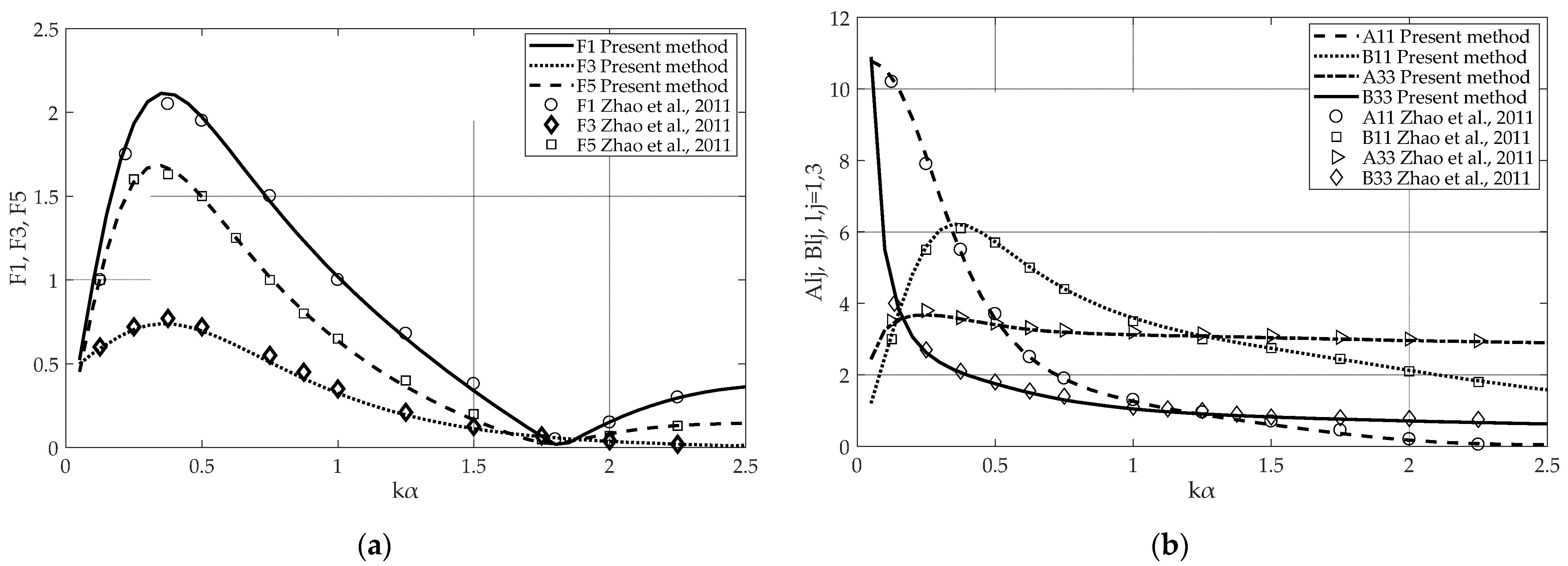
Considering the available literature, the theoretical results from the presented methodology are compared with the results from [34]. In the latter study, comprehensive comparisons between theoretical and experimental results were performed. Specifically, a 1:2 scaled down model of a permeable cylinder, made of steel, was tested in various wave slope conditions and wave periods, as well as in an impact test case restrained to the wave and one in forced heave oscillations.

The examined permeable cylindrical body of radius $a=0.15$ m and draught $d-h_1=0.3$ m is subjected to an incident wave train at a water depth $d=5$ m (see Figure 1). Here, the dimensionless porous effect parameter is equal to $G=1.432$, corresponding to an opening ratio of τ = 0.14 and wave steepness ε = 0.04633 (see Equation (3)). The validations of the results are made in terms of the dimensionless quantities of the surge, heave, and pitch wave exciting forces on the permeable body, i.e., ${\mathrm{F}}_l=\frac{\left|F_{\mathrm{l}}\right|}{\rho g{\alpha }^{2}H/2}, l=1,3$ and ${\mathrm{F}}_5=\frac{\left|F_5\right|}{\rho g{\alpha }^{3}H/2}$ (see Equations (29), (31), (33), and (34)). In addition, the dimensionless hydrodynamic coefficients (added masses $a_{11},a_{33}$ and hydrodynamic damping coefficients $b_{11},b_{33}$), i.e., ${\mathrm{A}}_{11,33}=\frac{a_{11,33}}{\rho {\alpha }^3}, {\mathrm{B}}_{11,33}=\frac{b_{11,33}}{\omega \rho {\alpha }^3}$ (see Equations (39) and (40)), are also compared.

Figure 3 depicts the exciting force components in surge, heave, and pitch for the selected value of $G$. Moreover, the added mass and the damping coefficients for the specific porous effect parameter are presented. It can be noted an excellent correlation between the results of the present methodology and the results from [32]. Consequently, the presented theoretical formulation can effectively simulate the effect of the permeable sidewall of a cylindrical body.

4.2. Numerical Results

In the sequel, a permeable cylindrical body of radius $a=35$ m is considered moored with a symmetrically arranged four-catenary-mooring-line system at a water depth $d=100$ m. The draught of the permeable sidewall is equal to $d-h_1=17.5$ m, whereas the thickness, $h_1-h$, of the impermeable bottom is assumed infinite (see Figure 1). To investigate the effect of porosity, five different sidewalls surfaces with different opening ratios are considered, i.e., $\tau =$ 0.05, 0.13, 0.2, 0.40, and 0.60. It is reminded that $\tau$ is defined as the ratio of the opened area to the total sidewall area. In addition, wave steepness $\epsilon =$ 0.05 is assumed. Hence, from Equation (3) the dimensionless porous effect parameters are equal to $G=$ 0.18, 1.22, 2.62, 8.92, and 17.48. The mass of the cylindrical body is assumed constant regardless the porosity of the sidewall surface, i.e., $M=$ 19.72 t, the center of gravity (CoG) is located at the body’s vertical axis, at 17.497 m below the water free surface, and the mass moment of inertia relative to water free surface equals to $I_z=$ 12,080 t·${\mathrm{m}}^2$.

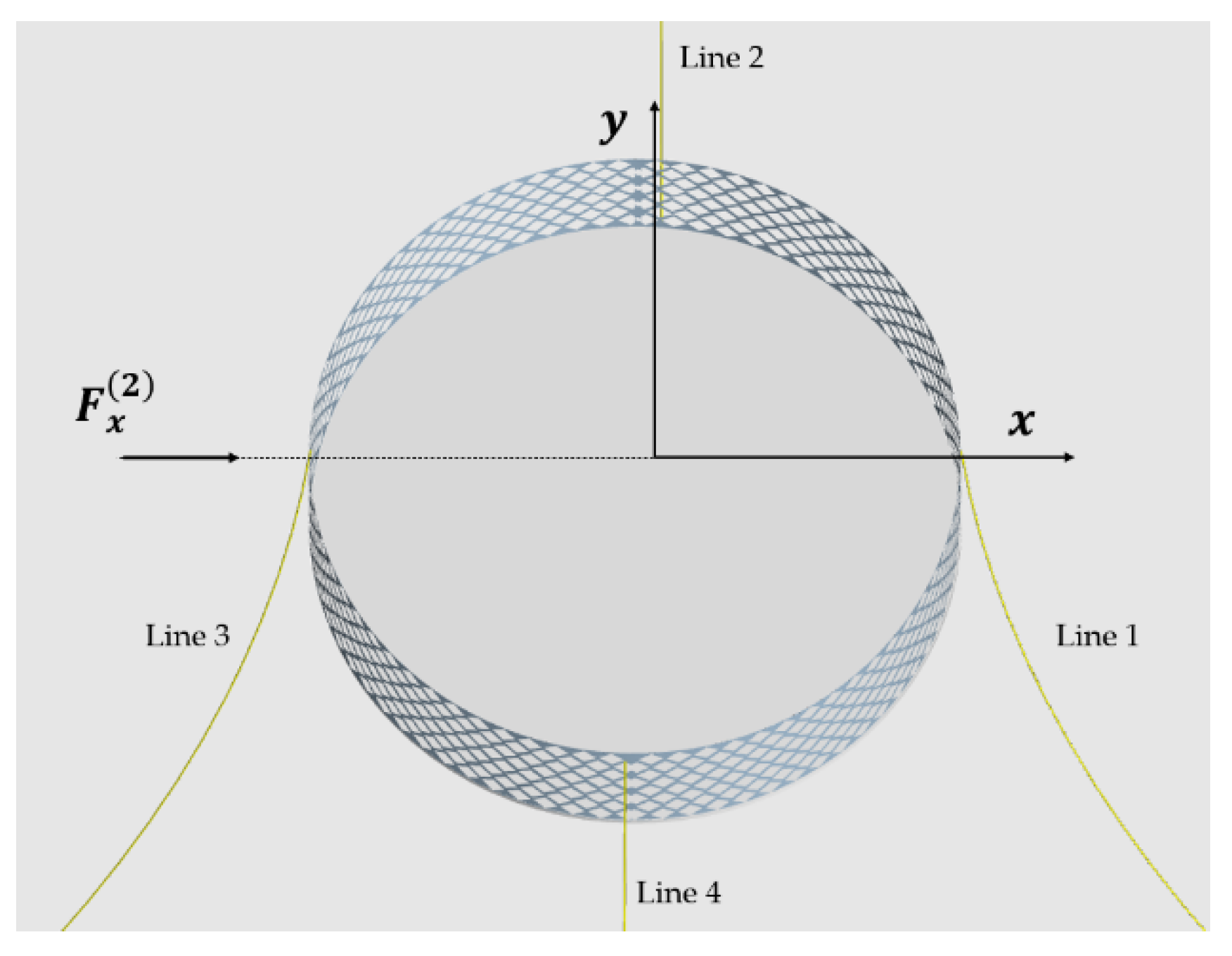
The examined permeable cylindrical body is anchored to the seabed through a symmetric mooring system, composed of four identical mooring lines (see Figure 4). The line’s mass is equal to 48.76 kg/m, whereas the submerged weight per meter of each line is $w=$ 415.25 N/m. The lines are assumed steel wires of diameter $d_m=100$ mm and of elasticity modulus $E=164.65$ GPa. The unstretched length of each line is $L=700$ m, and the minimum breaking tension is equal to 9147 kN. Furthermore, the formed angle by each line on the XY plane, with respect to the X-axis, is π/2.

The mooring system is initially considered to undergo only pretention loads. Continually, it is displaced from its initial equilibrium position under the action of horizontal environment forces $F_x^{\left(2\right)}=$ 300 kN.

Table 1. Mooring characteristics.

$w$	Submerged weight per unit length	415.25 N/m
$d$	Line diameter	0.1 m
$L$	Mooring length	700 m
$EA$	Axial stiffness	1.293 × 109 N
$F_x^{\left(2\right)}$	Horizontal environmental force	300 × 103 N
$l_B$	Bottom seated mooring length	79.11 m
$P_x^i$	$\mathrm{Horizontal}\mathrm{force}\mathrm{at}\mathrm{the}\mathrm{cable}\text{’}\mathrm{s}\mathrm{top},i=1,\dots ,4$	780 × 103 N
$P_z^i$	$\mathrm{Vertical}\mathrm{force}\mathrm{at}\mathrm{the}\mathrm{cable}’\mathrm{s}\mathrm{top},i=1,\dots ,4$	258 × 103 N
$x_B$	Horizontal projection of the suspended mooring line length	610.5 m
$c_{11}^m$	Mooring stiffness in x-direction due to the unit translational motion of its attachment point in the x-direction	135.9 kN/m
$c_{22}^m$	Mooring stiffness in y-direction due to the unit translational motion of its attachment point in the y-direction	1.27 kN/m
$c_{33}^m$	Mooring stiffness in z-direction due to the unit translational motion of its attachment point in the z-direction	4.84 kN/m
$c_{13}^m$	Mooring stiffness in x-direction due to the unit translational motion of its attachment point in the z-direction	21.87 kN/m

summarizes the mooring properties of each line, whereas, in

Table 2. Mooring attachment points.

	Line 1	Line 2	Line 3	Line 4
$a$	0	$\pi$/2	$\pi$	$3$/2
$x_m^i$	35	0	−35	0
$z_m^i$	0	0	0	0

, the locations of the attachment points of the lines on the cylindrical body in relation to the global coordinate system are presented.

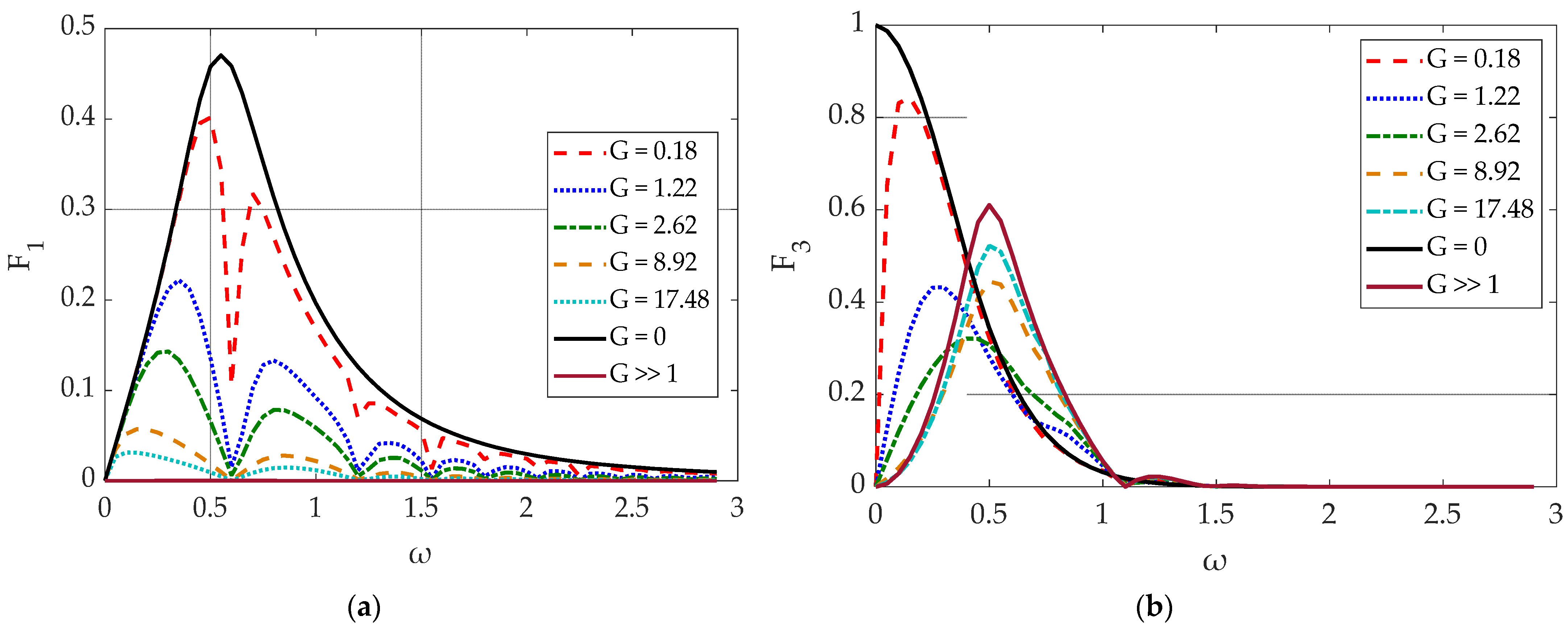
In Figure 5, the exciting forces on the permeable cylindrical body are presented for various values of porous effect parameter, i.e., $G=$ 0.18, 1.22, 2.62, 8.92, and 17.48. Here, $G=0$ and $G\gg 1$ are also considered. It should be reminded that, for $G=0$, the sidewall is assumed impermeable, whereas, for $G\gg 1$, the sidewall is considered fully permeable. The exciting forces are normalized by the terms ($\pi \rho g{\alpha }^{2}H/2$) and ($\pi \rho g{\alpha }^{3}H/2$), i.e., ${\mathrm{F}}_{\mathrm{l}}=\frac{\left|F_l\right|}{\pi \rho g{\alpha }^{2}H/2}, l=1,3$, and ${\mathrm{F}}_5=\frac{\left|F_5\right|}{\pi \rho g{\alpha }^{3}H/2}$. It can be seen from the figure that, as the porous effect parameter increases, the horizontal exciting forces decrease (see Figure 5a). Specifically, for a zero porous parameter (i.e., impermeable sidewall case) the horizontal exciting forces attain generally higher values than those for $G\ne 0$, since, in the latter case, the wave energy is absorbed by the permeable surface. It should also be noted a peculiar behavior of ${\mathrm{F}}_1$ at $\omega \approx 0.7;1.2;1.55,$ etc. This effect is notable for $G=$ 0.18, 1.22, 2.62, 8.92, and 17.48, whereas it is not depicted for $G=0$ and $G\gg 1$. In the vicinity of the corresponding wave frequencies, the ${\mathrm{F}}_1$ values attain a sharp decrease, which is more profound for lower values of $G$. The values of $ka$ at these wave frequencies are equal to 1.84, 5.33, and 8.53. These $ka$ values are in the neighborhood of the wave numbers which zero the derivative of the Bessel function of first kind, i.e., $J_1^{\prime }\left(ka\right)$. Hence, it can be concluded that sloshing phenomena do occur in permeable cylindrical bodies.

As far as the heave exciting forces presented in Figure 5b are concerned, it can be seen that, for $G=0$, the variation pattern of ${\mathrm{F}}_3$ differs from that for $G>0$. Specifically, for $G=0$, ${\mathrm{F}}_3$ tends to unity for ω tending to zero, whereas, for $G>0$, the vertical exciting force zeros when ω$\approx$ 0. Furthermore, the wave frequencies in which ${\mathrm{F}}_3$ attains local maxima are shifted to higher values as $G$ increases. Nevertheless, as ω increases (ω > 1), the effect of the porous effect parameter is no longer significant. Concerning the overturning moments (see Figure 5c), it can be seen that, at small wave frequencies (i.e., $\omega <0.4$), ${\mathrm{F}}_5$ increases reversely to $G$. On the other hand, for $\omega >0.4$, the moment ${\mathrm{F}}_5$ increases as $G$ increases, tending to the values of the submerged disc case (i.e., for $G\gg 1$). Moreover, for high values of ω, the porous effect parameter does not seem to affect ${\mathrm{F}}_5$.

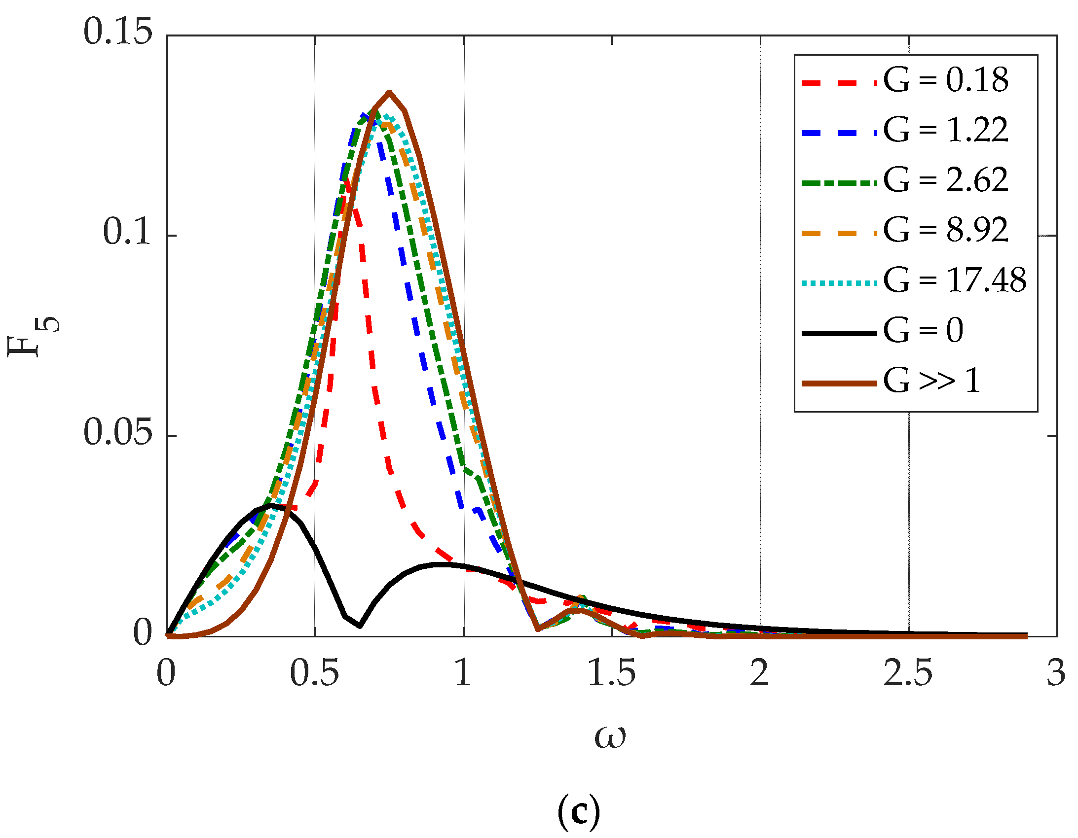
Figure 6 and Figure 7 depict the hydrodynamic coefficients of the examined permeable cylindrical body. The coefficients are normalized as ${\mathrm{A}}_{11,33}=\frac{a_{11,33}}{\rho {\alpha }^3}, {\mathrm{B}}_{11,33}=\frac{b_{11,33}}{\omega \rho {\alpha }^3}$, ${\mathrm{A}}_{15}=\frac{a_{15}}{\rho {\alpha }^4}, {\mathrm{B}}_{15}=\frac{b_{15}}{\omega \rho {\alpha }^4}$, and ${\mathrm{A}}_{55}=\frac{a_{55}}{\rho {\alpha }^5}, {\mathrm{B}}_{55}=\frac{b_{55}}{\omega \rho {\alpha }^5}$. Here, the cases of a truncated cylinder ($G=0$ case) and of a submerged cylindrical plate of infinite thickness ($G\gg 1$ case) are also considered. Regarding the added mass in surge direction, which is depicted in Figure 6a, it can be seen that ${\mathrm{A}}_{11}$ decreases as the porous effect parameter increases, tending to zero values for the submerged disc case. In addition, a sharp oscillation pattern can be seen at $\omega \approx 0.7;1.2;1.55,$ etc., which is more profound for lower values of $G$ corresponding to sloshing phenomena occurring in the case of partially porous bodies (see also discussion of Figure 5a). In Figure 6b, the added mass in heave ${\mathrm{A}}_{33}$ is depicted. It can be seen that, for ω < 0.7, the added mass behaves proportionally with $G$, since it increases as $G$ also increases tending to the values of the submerged plate case ($G\gg 1$). On the other hand, the effect of $G$ on the values of ${\mathrm{A}}_{33}$ can be considered negligible for ω > 0.7. The pitch ${\mathrm{A}}_{55}$ and surge pitch ${\mathrm{A}}_{15}$ added masses, depicted in Figure 6c,d, respectively, follow a similar rational to ${\mathrm{A}}_{11}$. Specifically, the tense oscillatory behavior at $\omega \approx 0.7;1.2;1.55,$ etc. is notable, which smoothens as $G$ increases. In addition, the values of ${\mathrm{A}}_{55},$ ${\mathrm{A}}_{15}$ tend to the corresponding values of the submerged plate case as $G$ increases. It should be noted that, due to symmetry,${\mathrm{A}}_{15}={\mathrm{A}}_{51}$, which also holds true for the permeable cylindrical bodies.

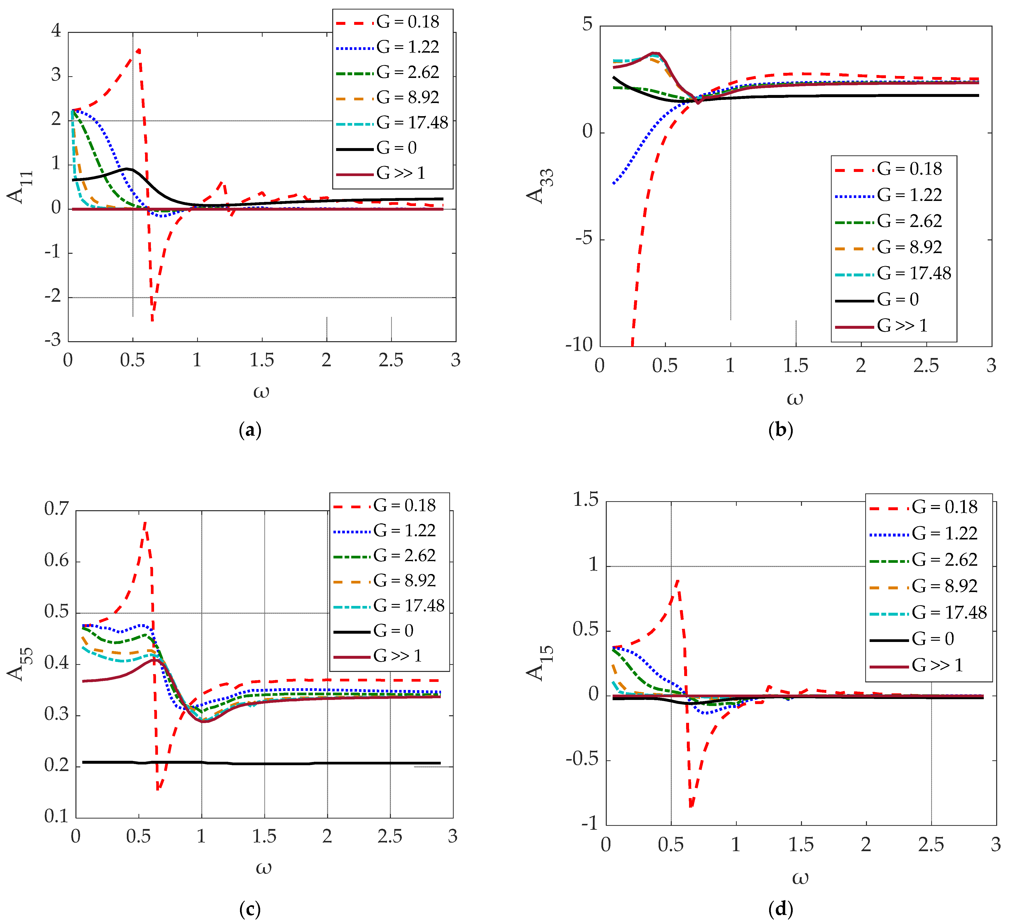
The effect of the porous parameter on the hydrodynamic damping coefficients of the examined permeable cylindrical body is shown in Figure 7, where the variations of ${\mathrm{B}}_{11},$ ${\mathrm{B}}_{33},{\mathrm{B}}_{55},$ ${\mathrm{B}}_{15}$ are presented versus the wave frequency. It can be seen from Figure 7a that ${\mathrm{B}}_{11}$ behaves reverse proportionally with $G$ for ω > 0.5. On the other hand, for small values of ω (i.e., ω < 0.5), the presented local maxima of ${\mathrm{B}}_{11}$ are shifted to lower values of ω as $G$ increases. Furthermore, the tense oscillatory behavior of ${\mathrm{B}}_{11}$ for small values of $G$ is also notable here, as in ${\mathrm{A}}_{11}$ (see Figure 6a). The variation of ${\mathrm{B}}_{33}$ is depicted in Figure 7b. The same conclusions can be drawn as in the ${\mathrm{A}}_{33}$ variation, concerning the decrease in ${\mathrm{B}}_{33}$ as $G$ increases, for small values of wave frequencies (ω < 0.25), as well as the negligible effect of $G$ on ${\mathrm{B}}_{33}$ for high values of ω (i.e., ω > 1). In Figure 7c,d, ${\mathrm{B}}_{55}$ and ${\mathrm{B}}_{15}$ are presented, respectively. It can be seen that the latter damping coefficients attain a similar tendency as ${\mathrm{A}}_{55}$ and ${\mathrm{A}}_{15}$ (see Figure 6c,d), regarding the decrease in the damping coefficients as the porous effect parameter increases, tending to the results of the submerged plate case. It also holds true that ${\mathrm{B}}_{15}={\mathrm{B}}_{51}$.

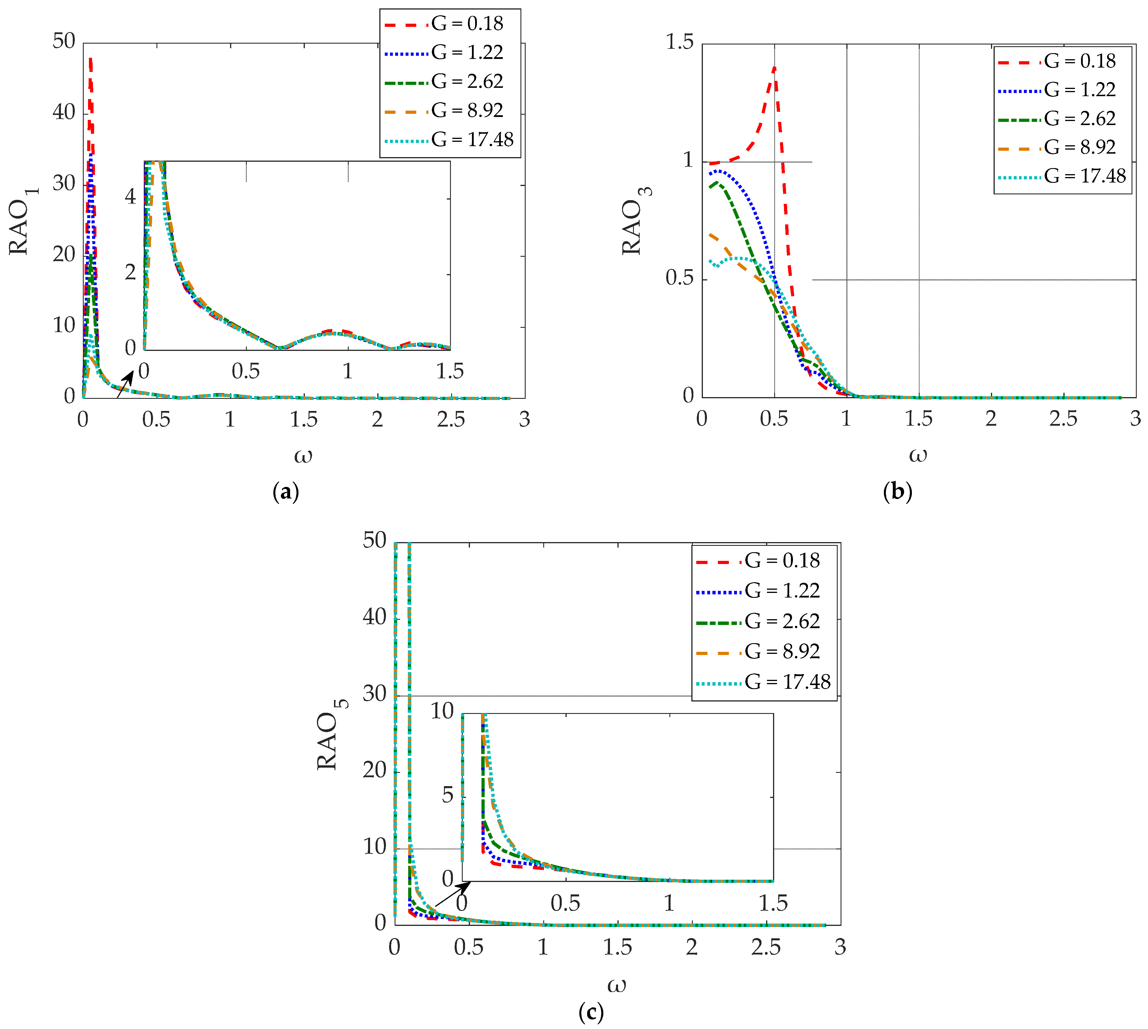
The effect of the porous parameter on the motions of the permeable cylindrical body is shown in Figure 8, where ${\mathrm{RAO}}_l, l=1,3,5,$ (see Equation (51)) is presented for various values of $G$. Here, a mooring quasi-static formulation is considered. The considered mooring characteristics are presented in Table 1. The mass of the body is equal to 19.72 t, regardless of the value of $G$, since the porous sidewall is assumed to be infinitesimally thin and have negligible mass. In the presented figures, the impermeable truncated cylinder and the submerged plate cases are not considered since they attain completely different mass and hydrostatic coefficients. Consequently, comparison of their motions with the corresponding ones of the examined permeable body seems meaningless.

Starting with the surge motions (Figure 8a), it can be seen that ${\mathrm{RAO}}_1$ variations behave reverse proportionally with $G$ for ω tending to zero (i.e., ω < 0.3). On the other hand, for ω > 0.3, the porous effect parameter seems to have a small effect on the body’s surge motions. Furthermore, the effect of the sloshing phenomena inside the porous sidewall on ${\mathrm{RAO}}_1$ is notable, minimizing the surge motion regardless the value of $G$ at $\omega \approx 0.7;1.2;1.55,$ etc. Concerning the maximization of ${\mathrm{RAO}}_1$, this can be traced back to the mooring restoring stiffness, which imposes a resonance location in the surge motion at ω$\approx 0.1$. The heave motions of the permeable cylindrical body are depicted in Figure 8b. It can be seen that ${\mathrm{RAO}}_3$ starts its variation from unity for ω tending to zero. Contrarily, as $G$ increases, the body’s heave displacement decreases, whereas, for ω > 1, the porous parameter attains a negligible effect on ${\mathrm{RAO}}_3.$ In Figure 8c, the body’s pitch motion is presented. In this figure, the mooring resonance at ω$\approx 0.1$ regardless of the values of $G$ should be noted, as well as the negligible effect of the sloshing phenomena on ${\mathrm{RAO}}_5.$

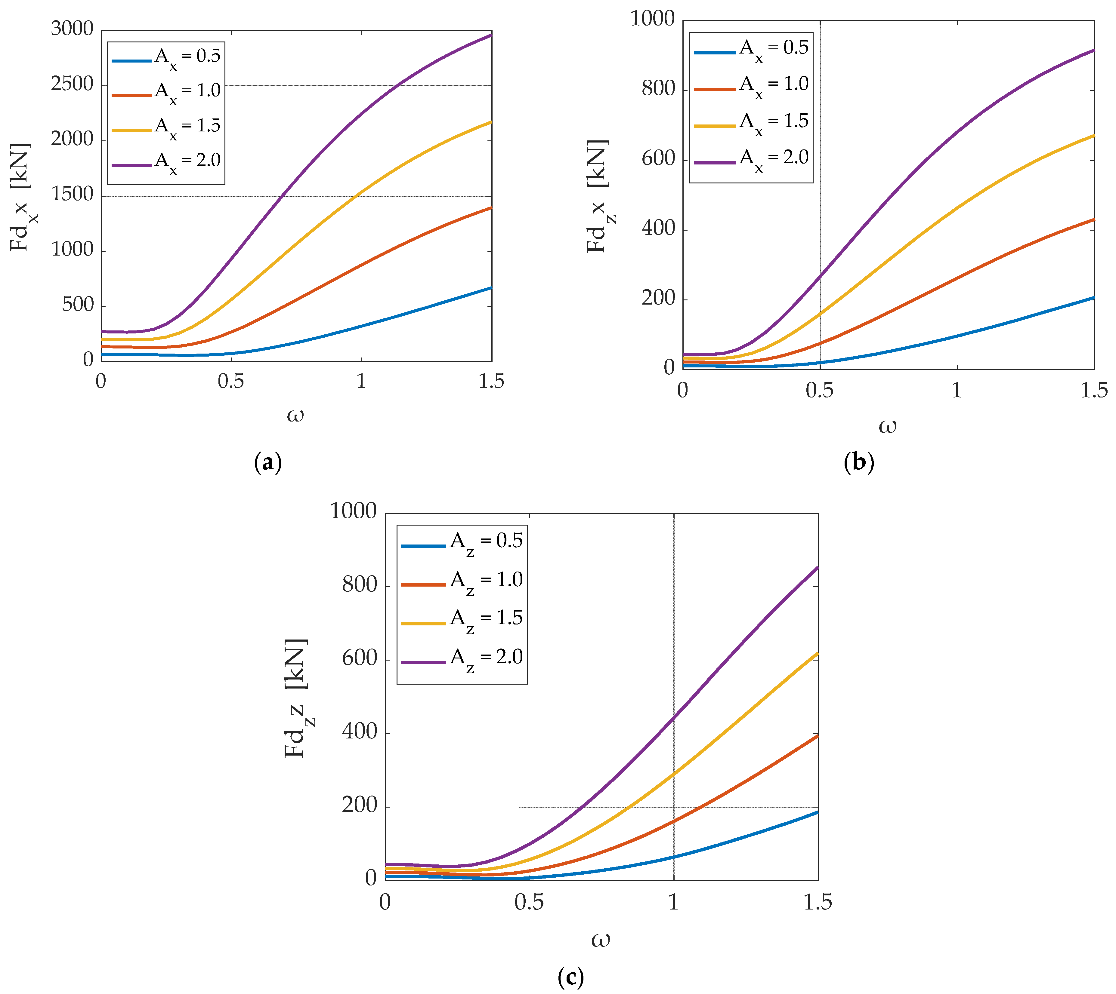
Next, the static analysis is extended by accounting for the lines’ dynamic behavior. Hence, the dynamic mooring damping and dynamic mooring restoring coefficients were evaluated and included in Equation (50). The followed procedure was described in Section 3.2. In Figure 9a,b the horizontal, ${\mathrm{Fd}}_{\mathrm{x}}\mathrm{x}=F_{11}^{d,1}$, and vertical, ${\mathrm{Fd}}_{\mathrm{z}}\mathrm{x}=F_{31}^{d,1}$, components of the dynamic tensions (see Equation (49)) at the top of the mooring line for horizontal sinusoidal motions of its upper end with amplitude ${\mathrm{A}}_1$ are presented. Similarly, in Figure 9c the corresponding vertical components of the dynamic tensions, ${\mathrm{Fd}}_{\mathrm{z}}\mathrm{z}=F_{33}^{d,1},$ at the top of the mooring line for vertical sinusoidal motions of amplitude ${\mathrm{A}}_3$ of its upper end are depicted. Here, ${\mathrm{A}}_{\mathrm{j}}=0.5, 1.0, 1.5, 2.0 \mathrm{m}, \mathrm{j}=1,3$. The considered mooring characteristics are presented in Table 1. The results of Figure 9 demonstrate clearly that the motion amplitude of the mooring upper end (i.e., connection point of each mooring line with the permeable cylindrical body) affects the dynamic tensions on the latter location. Specifically, the dynamic tensions for the particular inertia, the geometric mooring line characteristics, and the examined wave frequency range seem to behave proportionally with ${\mathrm{A}}_{\mathrm{j}}, \mathrm{j}=1,3$.

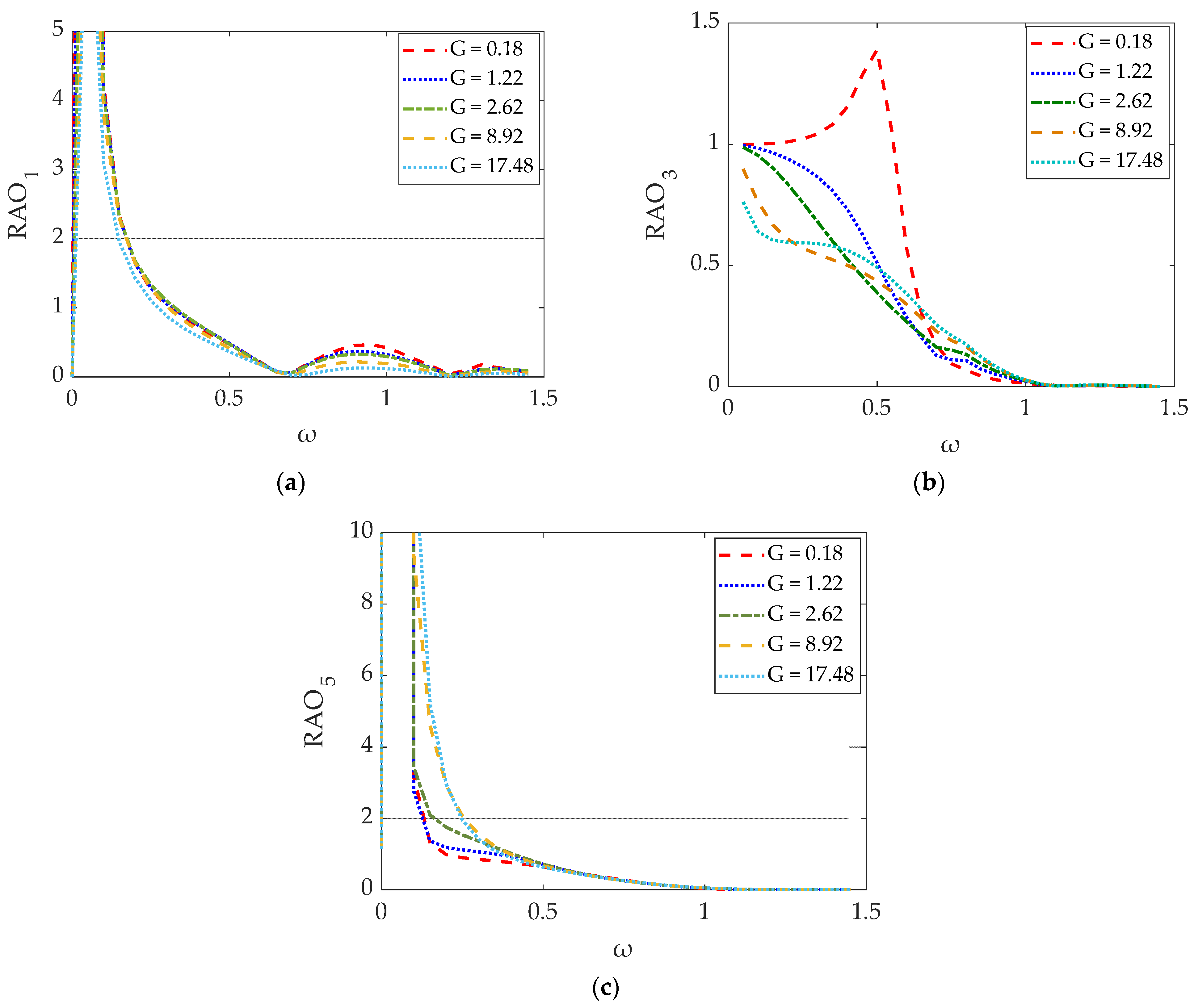
The effect of the dynamic mooring damping and dynamic mooring restoring coefficients on the permeable body’s motions for several porous effect parameters is shown in Figure 10, where the variations of ${\mathrm{RAO}}_l, l=1,3,5,$ (see Equation (51)) for $G=$ 0.18, 1.22, 2.62, 8.92, and 17.48 as a function of ω are depicted. Here, the dynamic mooring restoring coefficients and the dynamic dumping coefficient terms are considered in the solution of Equation (50) for the determination of the permeable body’s motions. In the followed iterative procedure, the horizontal and vertical components of the dynamic tension at the line’s top end, depicted in Figure 9 (see also Equation (49)), are coupled with the body’s motion equations (see Equation (50)) with a convergence coefficient $\epsilon =1 \times$10⁻¹⁰. In the case of surge response, ${\mathrm{RAO}}_1,$ (Figure 10a) the dynamic mooring lines stiffness, as well as the mooring damping consideration, lead to a small decrease in the values compared to the nondynamic case. This decrease is more profound for ω < 1.25, whereas this effect decreases for ω > 1.25. Nevertheless, ${\mathrm{RAO}}_1$ follows in general the pattern of the quasi-static case (see Figure 9a). Figure 10b depicts the variation of heave response. It can be seen that the dynamic characteristics of the mooring lines do not seem to affect the body’s vertical displacements, since ${\mathrm{RAO}}_3$ from the quasi-static analysis attains similar results to the dynamic case. The variation of ${\mathrm{RAO}}_5$ is shown in Figure 10c. A small decrease in pitch motions is also observed due to strong coupling between surge and pitch, which dictates a pattern of ${\mathrm{RAO}}_5$ similar to that of ${\mathrm{RAO}}_1$. Regarding the effect of $G$ on the pitch motions, it can be seen that the body’s rotations increase proportionally to the porous effect parameter. This is more profound for ω < 0.5. On the other hand, the effect of $G$ is negligible for ω > 0.5.

5. Conclusions

In the present paper, a moored permeable cylindrical body under the action of regular wave trains was investigated. Frequency analysis formulation was applied for the investigation of the effect of the porous parameter on the body’s hydrodynamics. Furthermore, the quasi-static and dynamic behavior of wire mooring lines on the body’s motions was studied. Special attention is given to the evaluation of dynamic stiffness and damping of the mooring lines through an iterative procedure. The presented numerical schemes account for the diffraction exciting forces and moments, the body’s hydrodynamic characteristics, and its translational and rotational motions. It is shown that the porous effect parameter plays a key role in reducing the wave loads on the permeable body by dissipating the wave energy. In addition, a small but significant decrease in the body’s surge and pitch motions is observed through the insertion of dynamic mooring characteristics on the system’s motion equation. On the other hand, the effect of the mooring dynamic characteristics on the body’s heave motion can be considered negligible.

The present theoretical formulation will be further developed in order to study the hydrodynamics of a moored cylindrical fish cage, similar to the examined permeable body, under the consideration of the sidewall’s flexibility in regular waves.

References

- Sollitt, C.; Cross, R. Wave transmission through permeable breakwaters. In Proceedings of the 13th Coastal Engineering Conference, Vancouver, BC, Canada, 10–14 July 1972; pp. 1827–1846. [Google Scholar]
- Madsen, O. Wave transmission through porous structures. J. Waterw. Ports Coast. Ocean. Eng. Div. 1974, 100, 169–188. [Google Scholar] [CrossRef]
- Solitt, C.; Cross, R. Wave Reflection and Transmission at Permeable Breakwaters; Tech. Paper 76-8; US Army Corps of Engineers, Coastal Engineering Research Center: Fort Belvoir, VA, USA, 1976. [Google Scholar]
- Sulisz, W. Wave reflection and transmission at permeable breakwaters of arbitrary cross section. Coast. Eng. 1985, 9, 371–386. [Google Scholar] [CrossRef]
- Pengzhi, L.; Karunarathna, S. Numerical study of solitary wave interaction with porous breakwaters. J. Waterw. Port Coast. Ocean. Eng. 2007, 133, 352–363. [Google Scholar]
- Huang, Z.; Li, Y.; Liu, Y. Hydraulic performance and wave loadings of perforated/slotted coastal structures: A review. Ocean Eng. 2011, 38, 1031–1053. [Google Scholar] [CrossRef]
- Lan, Y.; Hsu, T.; Lai, J.; Chwang, C.; Ting, C. Bragg scattering of waves propagating over a series of poro-elastic submerged breakwaters. Wave Motion 2011, 48, 1–12. [Google Scholar] [CrossRef]
- Liu, Y.; Li, H.J. Wave reflection and transmission by porous breakwaters: A new analytical solution. Coast. Eng. 2013, 78, 46–52. [Google Scholar] [CrossRef]
- Pereira, E.; The, H.; Manoharan, L.; Lim, C. Design optimization of porous box-type breakwater subjected to regular waves. MATEC Web Conf. 2018, 203, 01018. [Google Scholar] [CrossRef] [Green Version]
- Dai, J.; Wang, C.M.; Utsunomiya, T.; Duan, W. Review of recent research and developments on floating breakwaters. Ocean Eng. 2018, 158, 132–151. [Google Scholar] [CrossRef]
- Han, M.M.; Wang, C.M. Hydrodynamics study on rectangular porous breakwater with horizontal internal water channels. J. Ocean Eng. Mar. Energy 2020, 6, 377–398. [Google Scholar] [CrossRef]
- Kawakami, T. The theory of designing and testing fishing nets in model. In Modern Fishing Gear of the World (2); Fishing News (Books) Ltd.: London, UK, 2006; pp. 471–481. [Google Scholar]
- Aarsnes, J.V.; Rudi, H.; Loland, G. Current forces on cage, net deflection. Engineering for offshore fish farming. In Proceedings of the a Conference Organized by the Institution of Civil Engineers, Glasgow, UK, 17–18 October 1990. [Google Scholar]
- Bessonneau, J.S.; Marichal, D. Study of the dynamics of submerged supple nets (applications to trawls). Ocean. Eng. 1998, 25, 563–583. [Google Scholar] [CrossRef]
- Cho, I.H.; Kim, M.H. Interactions of horizontal porous flexible membrane with waves. J. Waterw. Port Coast. Ocean Eng. 2000, 126, 245–253. [Google Scholar] [CrossRef]
- Chan, A.; Lee, S.W.C. Wave characteristics past a flexible fishnet. Ocean Eng. 2001, 28, 1517–1529. [Google Scholar] [CrossRef]
- Wan, R.; Hu, F.; Tokai, T. A static analysis of the tension and configuration of submerged plane nets. Fish. Sci. 2002, 68, 815–823. [Google Scholar] [CrossRef]
- Tagaki, T.; Suzuki, K.; Hiraishi, T. Development of the numerical simulation method of dynamic fishing net shape. Nippon Suisan Gakkaishi 2002, 68, 320–326. [Google Scholar] [CrossRef] [Green Version]
- Fredheim, A.; Faltinsen, O.M. Hydroelastic analysis of a fishing net in steady inflow conditions. In Proceedings of the 3rd International Conference on Hydroelasticity in Marine Technology 2003, Oxford, UK, 15–17 September 2003. [Google Scholar]
- Bao, W.; Kinoshita, T.; Zhao, F. Wave forces acting on a semi-submerged porous circular cylinder. Proc. Inst. Mech. Eng. Part M J. Eng. Marit. Environ. 2009, 223, 349–360. [Google Scholar] [CrossRef]
- Faltinsen, O.M. Hydrodynamic aspects of a floating fish farm with circular collar. In Proceedings of the 26th International Workshop on Water Waves and Floating Bodies (IWWWFB 2011), Athens, Greece, 17–20 April 2011. [Google Scholar]
- Kristiansen, T.; Faltinsen, O.M. Modelling of current loads on aquaculture net cages. J. Fluids Struct. 2012, 34, 218–235. [Google Scholar] [CrossRef]
- Kristiansen, T.; Faltinsen, O.M. Experimental and numerical study of an aquaculture net cage with floater in waves and current. J. Fluids Struct. 2015, 54, 1–26. [Google Scholar] [CrossRef] [Green Version]
- Shen, Y.G.; Greco, M.; Faltinsen, O.M.; Nygaard, I. Numerical and experimental investigations on mooring loads of a marine fish farm in waves and current. J. Fluids Struct. 2018, 79, 115–136. [Google Scholar] [CrossRef]
- Ito, S.; Kinoshita, T.; Bao, W. Hydrodynamic behaviors of an elastic net structure. Ocean Eng. 2014, 92, 188–197. [Google Scholar] [CrossRef]
- Mandal, S.; Sahoo, T. Wave interaction with floating flexible circular cage system. In Proceedings of the 11th International Conference on Hydrodynamics (ICHD 2014), Singapore, 19–24 October 2014. [Google Scholar]
- Su, W.; Zhan, J.M.; Huang, H. Wave interactions with a porous and flexible cylindrical fish cage. Procedia Eng. 2015, 126, 254–259. [Google Scholar] [CrossRef] [Green Version]
- Ma, M.; Zhang, H.; Jeng, D.S.; Wang, C.M. A semi-analytical model for studying hydroelastic behaviour of a cylindrical net cage under wave action. J. Mar. Sci. Eng. 2021, 9, 1445. [Google Scholar] [CrossRef]
- Liu, Z.; Mohapatra, S.C.; Guedes Soares, C. Finite element analysis of the effect of currents on the dynamics of a moored flexible cylindrical net cage. J. Mar. Sci. Eng. 2021, 9, 159. [Google Scholar] [CrossRef]
- Ma, M.; Zhang, H.; Jeng, D.S.; Wang, C.M. Analytical solutions of hydroelastic interactions between waves and submerged open-net fish cage modeled as a porous cylindrical thin shell. Phys. Fluids 2022, 34, 017104. [Google Scholar] [CrossRef]
- Williams, A.N.; Li, W. Water wave interaction with an array of bottom-mounted surface-piercing porous cylinders. Ocean Eng. 2000, 27, 841–866. [Google Scholar] [CrossRef]
- Williams, A.N.; Li, W.; Wang, K.H. Water wave interaction with a floating porous cylinder. Ocean Eng. 2000, 27, 1–28. [Google Scholar] [CrossRef]
- Park, M.S.; Koo, W.; Choi, Y. Hydrodynamic interaction with an array of porous circular cylinders. Int. J. Nav. Archit. Ocean Eng. 2010, 2, 146–154. [Google Scholar] [CrossRef] [Green Version]
- Zhao, F.; Bao, W.; Kinoshita, T.; Itakura, H. Theoretical and experimental study on a porous cylinder floating in waves. ASME J. Offshore Mech. Arct. Eng. 2011, 133, 011301. [Google Scholar] [CrossRef]
- Zhao, F.; Kinoshita, T.; Bao, W.G.; Huang, L.Y.; Liang, Z.; Wan, R. Interaction between waves and an array of floating porous circular cylinders. China Ocean Eng. 2012, 26, 397–412. [Google Scholar] [CrossRef]
- Park, M.S.; Koo, W. Mathematical modeling of partial-porous circular cylinders with water waves. Hindawio Publishing Corporation. Math. Probl. Eng. 2015, 2015, 903748. [Google Scholar] [CrossRef]
- Dokken, J.; Grue, J.; Karstensen, P. Wave analysis of porous geometry with linear resistance law. J. Mar. Sci. Appl. 2017, 16, 480–489. [Google Scholar] [CrossRef] [Green Version]
- Dokken, J.; Grue, J.; Karstensen, P. Wave forces on porous geometries with linear and quadratic pressure-velocity relations. In Proceedings of the 32nd International Workshop on Water Waves and Floating Bodies, IWWWFB, Dalian, China, 23–26 April 2017. [Google Scholar]
- Cong, P.; Bai, W.; Teng, B. Analytical modeling of water wave interaction with bottom-mounted surface-piercing porous cylinder in front of a vertical wall. J. Fluids Struct. 2019, 88, 292–314. [Google Scholar] [CrossRef]
- Qiao, D.; Mackay, E.; Yan, J.; Feng, C.; Li, B.; Feichtner, A.; Ning, D.; Johanning, L. Numerical simulation with a macroscopic CFD method and experimental analysis of wave interaction with fixed porous cylinder structures. Mar. Struct. 2021, 80, 103096. [Google Scholar] [CrossRef]
- Kokkinowrachos, K.; Mavrakos, S.A.; Asorakos, S. Behavior of vertical bodies of revolution in waves. Ocean Eng. 1986, 13, 505–538. [Google Scholar] [CrossRef]
- Konispoliatis, D.; Chatjigeorgiou, I.; Mavrakos, S. Theoretical hydrodynamic analysis of a surface-piercing porous cylindrical body. Fluids 2021, 6, 320. [Google Scholar] [CrossRef]
- Sankar, A.; Bora, S.N. Hydrodynamic coefficients for a floating semi-porous compound cylinder in finite ocean depth. Mar. Syst. Ocean Technol. 2020, 15, 270–285. [Google Scholar] [CrossRef]
- Sankar, A.; Bora, S.N. Hydrodynamic forces and moments due to interaction of linear water waves with truncated partial-porous cylinders in finite depth. J. Fluids Struct. 2020, 94, 120898. [Google Scholar]
- Abramowitz, M.; Stegun, I.A. Handbook of Mathematical Functions, 9th ed.; Dover Publication: Washington, DC, USA, 1970. [Google Scholar]
- Mavrakos, S.A.; Chatjigeorgiou, I.K. Mooring-induced damping on floating structures. In Proceedings of the 1st International Conference on Marine Industry, Varna, Bulgaria, 2–7 June 1996; Volume II, pp. 365–378. [Google Scholar]
- Triantafyllou, M.S. Preliminary design of mooring systems. J. Ship Res. 1982, 26, 25–35. [Google Scholar] [CrossRef]
- Triantafyllou, M.S.; Bliek, A.; Shin, H. Static and Fatigue Analysis of Multi-Leg Mooring Systems; Technical report; MIT Press: Cambridge, MA, USA, 1986. [Google Scholar]
- Amaechi, C.V.; Wang, F.; Ye, J. Numerical studies on CALM buoy motion responses and the effect of buoy geometry cum skirt dimensions with its hydrodynamic waves—Current interactions. Ocean. Eng. 2022, 244, 110378. [Google Scholar] [CrossRef]
- Loukogeorgaki, E.; Angelides, D. Stiffness of mooring lines and performance of floating breakwater in three dimensions. Appl. Ocean Res. 2005, 27, 187–208. [Google Scholar] [CrossRef]
- Mavrakos, S.A. User’s manual for the computer code HAMVAB. In Laboratory for Floating Bodies and Mooring Systems; National Technical University of Athens: Athens, Greece, 2001. [Google Scholar]
Figure 1.
A 3D representation of the examined permeable vertical cylindrical body.
Figure 2.
Representation of mooring cable and global coordinate system: (a) schematic representation of a 2D typical mooring line; (b) depiction of the mooring cable and global coordinate system orientation.
Figure 3.
Comparison of the present analytical results with Zhao et al. [32] in terms of (a) dimensionless exciting forces
and (b) dimensionless hydrodynamic coefficients . Here, .
Figure 4.
A 3D representation of the examined symmetric mooring system, composed by four identical mooring lines.
Figure 5.
Dimensionless exciting forces on the permeable cylindrical body against wave frequency for various values of porous effect parameter 0.18, 1.22, 2.62, 8.92, and 17.48: (a) ; (b) ; (c) . Here, and cases are also presented.
Figure 6.
Dimensionless hydrodynamic added mass of the permeable cylindrical body against wave frequency for various values of porous effect parameter: (a) ; (b) ; (c) ; (d) . The results are also compared with the corresponding ones of a truncated cylinder ( case) and of a submerged cylindrical plate ( case).
Figure 7.
Dimensionless hydrodynamic damping coefficients of the permeable cylindrical body against wave frequency for various values of porous effect parameter: (a) ; (b) ; (c) ; (d) . The results are also compared with the corresponding ones of a truncated cylinder ( case) and of a submerged cylindrical plate ( case).
Figure 8.
Dimensionless motions of the permeable cylindrical body against wave frequency for various values of porous effect parameter 0.18, 1.22, 2.62, 8.92, and 17.48: (a) ; (b) ; (c) .
Figure 9.
Horizontal and vertical dynamic tensions at the top of the mooring line against wave frequency for various values of horizontal motion amplitudes m: (a) ; (b) ; (c) .
Figure 10.
Dimensionless motions of the permeable cylindrical body against wave frequency for various values of porous effect parameter 0.18, 1.22, 2.62, 8.92, and 17.48: (a) ; (b) ; (c) . Here, the dynamic mooring
characteristics were taken into consideration.