Artificial Intelligence as a Tool to Study the 3D Skeletal Architecture in Newly Settled Coral Recruits: Insights into the Effects of Ocean Acidification on Coral Biomineralization

Abstract

Understanding the formation of the coral skeleton has been a common subject uniting various marine and materials study fields. Two main regions dominate coral skeleton growth: Rapid Accretion Deposits (RADs) and Thickening Deposits (TDs). These have been extensively characterized at the 2D level, but their 3D characteristics are still poorly described. Here, we present an innovative approach to combine synchrotron phase contrast-enhanced microCT (PCE-CT) with artificial intelligence (AI) to explore the 3D architecture of RADs and TDs within the coral skeleton. As a reference study system, we used recruits of the stony coral Stylophora pistillata from the Red Sea, grown under both natural and simulated ocean acidification conditions. We thus studied the recruit’s skeleton under both regular and morphologically-altered acidic conditions. By imaging the corals with PCE-CT, we revealed the interwoven morphologies of RADs and TDs. Deep-learning neural networks were invoked to explore AI segmentation of these regions, to overcome limitations of common segmentation techniques. This analysis yielded highly-detailed 3D information about the RAD’s and TD’s architecture. Our results demonstrate how AI can be used as a powerful tool to obtain 3D data essential for studying coral biomineralization and for exploring the effects of environmental change on coral growth.

1. Introduction

In tropical and subtropical oceans, symbiotic stony corals provide an ecological framework that retains nutrients, support high rates of autotrophic production, and harbor extensive biological diversity. The skeletons, created by tiny coral polyps in colonies, are known to be among the largest bioconstructions in the world. Understanding the details of structure generation and principles of coral skeletal formation have been a common topic among diverse fields of study including biology, geochemistry, geology, paleontology, and materials science. The skeletons of stony corals consist of two main skeletal regions known as Rapid Accretion Deposits (RADs; also known as “calcification centers”) and Thickening Deposits (TDs; also called “fibers”). RADs correspond to areas of the skeleton with rapid calcium carbonate deposition where new skeletal growth zones start to form [1,2,3]. They contain an organic matrix and consist of granular aggregates that comprise randomly oriented calcium carbonate crystals containing both aragonite and stable amorphous calcium carbonate [4,5,6]. A second calcium carbonate form, Mg-calcite, has been shown to also be present in the early stages of RADs formation, typical of initial mineral development in early coral life stages [7]. Outward from RADs, the mineral grows into TDs, forming elongated aragonite crystals with a fibrous morphology appearing compact and dense with significantly reduced amounts of organics as compared to RADs [2,3,8,9,10,11].

The coral skeleton has been well characterized at the micro-structural level [2,3,4,5,8,9,10,11,12,13], but less is known about how changes in the environment may affect its development, in particular regarding the formation of RADs and TDs. Recent predictions suggest that future ocean acidification (OA) conditions, resulting in a chemical shift toward higher seawater pCO₂ and lower pH, will significantly hinder the coral mineral formation and overall skeletal growth [14,15,16,17,18]. In the early stages of coral life, we have recently shown that exposure to future OA conditions causes a reduction in the abundance of RADs in the skeletal spines [19]. However, previous results relied solely on scanning electron microscope (SEM) images; hence, they were limited only to two-dimensional (2D) surface observations. Indeed, most studies on coral skeletal structures make use of 2D-based microscopy analyses [1,2,3,8,9,11,12,13,20], which lack volumetric quantifications. Therefore, the lack of an appropriate methodology to precisely visualize the volumetric configuration of RADs and TDs has limited investigation of the 3D structure of these two skeletal regions [3,11,21].

Following the widespread development of high-resolution X-ray µCT in medical and industrial applications, non-destructive imaging of 3D structures has become popular. It is thus possible to monitor mineral internal structural changes [22] and characterization [23] at resolutions down to a few tens of nanometers. Conventional X-ray µCT imaging methods mainly rely on X-ray absorption as a mechanism to generate images based on the attenuation of the X-rays by the material, yielding spatial information about density distributions within the sample. This technique, however, is prone to normalization artifacts and does not distinguish between materials with very similar X-ray attenuation [24,25]. Other methods such as phase contrast-enhanced microCT (PCE-CT) exploit differences in X-ray interaction to create high-contrast images where even small differences in density along the X-ray path can lead to strong contrast enhancement at interfaces between material phases [24]. PCE-CT imaging can thus highlight edges and internal boundaries in intact samples, even in the case of quite similar material compositions [24]. These characteristics of PCE-CT make it a good candidate for enhancing the visibility of RADs and TDs and ease their identification within the coral skeleton.

For a detailed analysis of microstructures, volumetric quantification techniques must be applied with the capacity to accurately differentiate and represent individual material phases. In recent years, several works have shown that artificial intelligence (AI) algorithms can be applied for visual classification tasks such as in the case of materials with complex microstructures [26,27,28]. These applications make increasing use of machine learning methods based on Deep Learning (DL) neural networks. DL networks comprise a large number of interconnected processors (neurons) that work in parallel [29]. For visual classification, the network is trained to identify structures of interest using a training “ground truth” dataset, which is used by the computer as a reference to classify similar images. The process is known as supervised classification, and has been employed in µCT images of minerals to visualize and characterize 3D structures with high accuracy [30,31,32,33].

In the present study, we combine AI and PCE-CT to obtain quantitative information about the density and 3D distribution of RADs and TDs within coral skeletons imaged with phase contrast enhancement. Such information is currently unavailable using conventional 2D or other imaging methods. We used coral primary polyps as the study system for the development of a robust analytic 3D quantification methodology, since rapid calcification during initial life stages of stony corals provides a unique opportunity to study the formation of calcium carbonate that involves extensive skeleton morphological changes. In addition, the early stages of coral development represent a good candidate to test the performance of our approach under experimental conditions that we know induce alterations in the development of RADs, such as exposure to OA conditions [19].

To develop our new methodology and optimize its performance across varied conditions, we analyzed high resolution scans of the skeletal structures of recruits of an abundant stony coral species Stylophora pistillata from the Red Sea, following settlement and growth under both natural and OA conditions. In particular, we simulated the global mean surface-ocean decline in pH predicted to occur under the RCP8.5 scenario [34] by the end of this century (pH drop ca. 0.1–0.4 units, from ~8.0 to 7.6; [35]). Employing PCE-CT, we identified the μm-sized edges of RADs and TDs within the skeleton. The high-contrast images generated with PCE-CT allowed us to use AI to segment RADs and TDs, under both natural conditions and under what we expect to be morphologically-altered OA conditions, and to reproduce these structures in 3D with quantitative detail.

2. Materials and Methods

2.1. Sample Collection and OA Experiment

Coral larvae were collected from 15 randomly selected adult colonies of the stony coral S. pistillata on the reef adjacent to the Interuniversity Institute of Marine Sciences (IUI, 29°30′06.0″ N 34°54′58.3″ E) in the Gulf of Eilat (Israel), under a permit from the Israeli Natural Parks Authority. Larvae were collected using dedicated traps (160 µm plankton net with a plastic collection container) that were placed on adult colonies from the shallow reef (depth 6–7 m) for several nights of spawning during April 2020.

All actively swimming larvae were pooled together and were transported to a controlled environment aquarium system at the Leon H. Charney School of Marine Science (University of Haifa, Haifa, Israel). Larvae were placed in custom-made polypropylene plastic chambers (~20 larvae per chamber) consisting of a central cylinder sealed at the ends by plankton netting. Settlement chambers were used in this experiment to avoid losing larvae through the water recycle system of the aquariums before settlement, as previously reported [19,36,37]. Prior to the insertion of the larvae, the chambers were washed to remove any potential chemical released by the plastic, and they were left to soak in seawater for one week.

The settlement chambers (1 chamber per aquarium) were placed in a system of 6 flow-through aquariums with artificial seawater (Red Sea Salt, Red Sea Ltd., Houston, TX, USA) replicating the spring northern Red Sea water conditions as previously described [19]: pH of 8.19 ± 0.01 (seasonal mean ± s.d.), salinity of 40.63 ± 0.03 g L⁻¹ (seasonal mean ± s.d.), and temperature of 22.18 ± 0.17 °C (seasonal mean ± s.d.). An irradiance of 250 μmol photons m⁻² s⁻¹ on a 12-h light-dark cycle was provided by a Mitras LX 7206 LED aquarium light system (GHL, Kaiserslautern, Germany).

Prior to the insertion of the settlement chambers, the carbonate chemistry of seawater was manipulated in 3 of the experimental aquariums by injecting CO₂ to reduce the ambient pH 8.2 (pCO₂~487 µatm) and obtain the target value of pH 7.6 (pCO₂~1938 µatm). Temperature and salinity were monitored continuously throughout the experiment by electrodes linked to a monitoring system (GHL, Kaiserslautern, Germany) that controlled CO₂ injection, and they were also measured three times per day using a portable Orion Star™ A222 conductivity meter (Thermo Fisher Scientific, Waltham, MA, USA). Measurements of pH (NBS scale) were performed three times per day using a pH glass electrode (Metrohm, Herisau, Switzerland) where buffer solutions (Rocker Scientific, Taiwan) were employed to perform calibration (pH 4, pH 7, and pH 10). Measurements of total alkalinity (TA) were made once per day (triplicates) via titration with 0.1 N HCl containing 40.7 g NaCl L⁻¹, using an automatic alkalinity titrator (855 Robotic Titrosampler, Metrohm, Herisau, Switzerland) controlled by Tiamo (Software version 2.0, Metrohm, Herisau, Switzerland). Automated titrations of 50 mL samples were performed. Parameters of seawater carbonate system were calculated from pH, TA, temperature, and salinity using the CO2SYS package [38] with constants from [39] as refit by [40] (Supplemental Table S1). Throughout the experiment, corals were fed once per day with 2 mL of concentrated planktonic suspension (Microvore, Brightwell R aquatics, Fort Payne, AL, USA). The experiment lasted for a total of 9 days, following our previous experimental procedure [19], after which primary polyps were gently removed from the chambers and stored with 90% ethanol in 2 mL tubes.

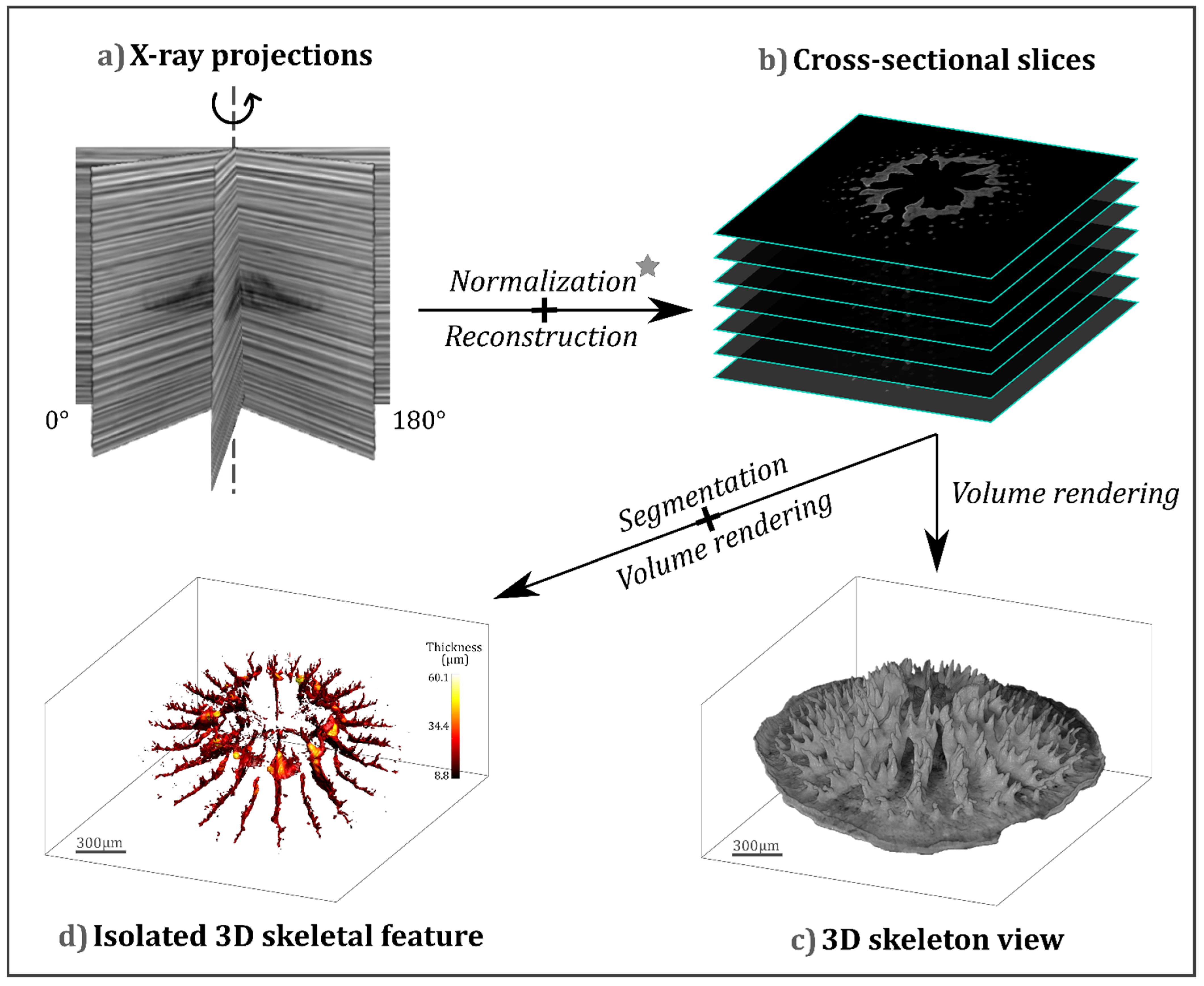
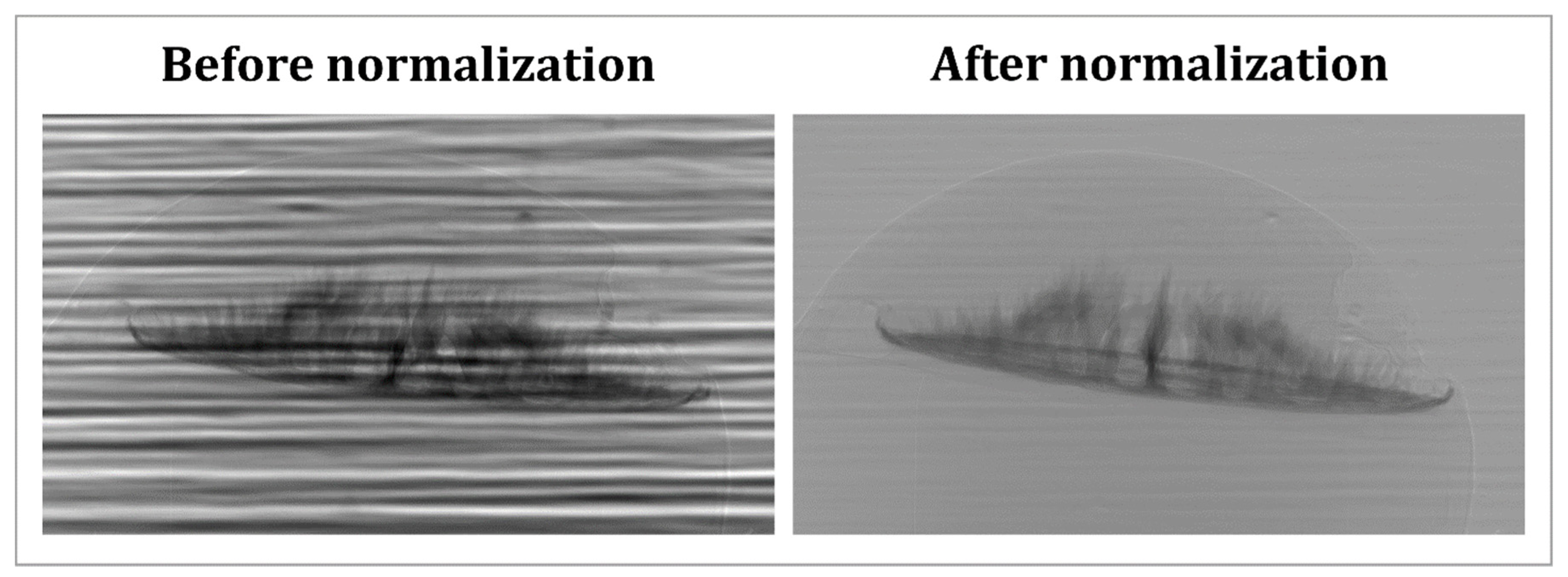
2.2. X-ray µCT: Image Acquisition and Tomographic Reconstruction

Primary polyps were fixed with EpoFix resin (Agar Scientific, Stansted, UK) on top of polypropylene micropipette tips. Tomographic scanning was conducted at BAMline [41,42], the imaging beamline of BESSY II (the synchrotron storage ring of HZB—Helmholtz-Zentrum Berlin, Germany). Each sample (N = 3 per pH treatment) was attached to a metal stub and scanned with incremental rotation (multiple projections spanning 180°) (Figure 1a) using the high-resolution imaging setup (Supplemental Figure S1) [43] with exposure times set to 1 s. Projection images were acquired with a final pixel size of 2.2 µm using PCE-CT imaging mode at an energy of 24.5 keV. Additional absorption scans were performed for comparison, using an energy of 16.26 keV, to ensure correct identification of the skeletal structures avoiding contrast enhancement.

Prior to reconstruction, data were normalized to account for beam inhomogeneities using an in-house Octave-based reconstruction pipeline in the labs of the Charité, Universitätsmedizin (Berlin, Germany). Specifically, for each scan, the radiograms were background-corrected by normalization with best-fitting (minimum variance) empty beam (flat-field) images, obtained both before and after each scan, and corrected by subtraction of dark-current images (Figure 2). Reconstruction was performed by the filtered back projection method using nRecon (v 1.7.4.2, Brucker micro-CT, Kontich, Belgium) to generate 3D datasets from cross-sectional 2D images (Figure 1b). Tomographic datasets were visualized and further processed in 3D using Dragonfly (v 2021.3, Object Research Systems—ORS, Montreal, Quebec, Canada) (Figure 1c,d) [44], with additional stack analyses performed in FIJI [45].

2.3. Deep-Learning-Based Image Segmentation

To objectively identify structures in the PCE tomographic data, each reconstruction was segmented using the Deep Learning functions built into the 3D commercially-available software Dragonfly (v2021.3, Object Research Systems—ORS, Montreal, Quebec, Canada) [46]. Segmentation is necessary for the processes of analysis and quantification of the volume of RADs and TDs with respect to the total volume of the skeleton (mineral excluding air cavities) of each primary coral polyp scanned. This process is required to partition digital images into several sub-volumes, each representing a distinct 3D feature, obtained by identification and grouping of similar volume pixels (voxels) [47]. Image segmentation is thus typically used to locate objects of interest in large volumes of data needing quantification. In the present study, we applied semantic image segmentation by labeling and grouping pixels in each slice-image according to the feature that they were part of (RADs, TDs, or air spaces). For this classification, we used the U-Net network architecture algorithm, which has been shown to be very efficient in segmenting biomedical images [48]. When applying supervised classification, the network is manually trained by providing examples of how different features within the data should be classified. This is achieved by manually selecting groups of voxels and assigning them to a specific feature within a set of representative images, considered to be a training dataset. The computer then uses the manually-segmented training datasets as reference for automatic classification of all other regions in all images. We therefore manually delineated RADs, TDs, and air spaces in several (<10) 2D slices within each reconstructed tomographic dataset. These were used to train the network to recognize different features within all other images (Figure 3a–d).

Training requires optimizing a series of parameters that define the performance of the U-Net network workflow. Within the Dragonfly platform, several parameters can be tuned: (1) patch size (images are split into smaller rectangular patches that contain the feature of interest [49]), (2) stride-to-input ratio (a parameter defining the typical position relationships between neighboring patches), (3) batch size (the number of patches evaluated concomitantly), (4) number of epochs (cycles of iteration that involve computation of all batches of the training dataset), (5) loss function (which measures the difference between groups of voxels in the training set images, considered to be “the ground truth images”, and the output value predicted by the network [50]), (6) optimization algorithm (different approaches to minimize the loss function, and thus to reduce the training error), and (7) data augmentation (how many times each data patch is augmented during a single training epoch). In this work, optimization of the DL network performance was achieved by making trial runs with different combinations of number of training slices and of the above-mentioned values of network parameters (starting with default settings provided at first by the software), until reaching reproducible accuracy of the segmentation (a single user ensured by visual examination that the trained network accurately segmented skeletal regions, by comparison to the ground truth images, i.e., the training set of images). The final optimized workflow thus required training datasets of 8 to 11 slices and a series of parameters (1–6 as described above) set to: (1) 32, (2) 1, (3) 32, (4) 100, (5) OrsDiceLoss, (6) Adadelta, and (7) 2. The trained network was then applied to segment all slices within each tomographic stack (Figure 3e). The segmented skeletal structures were visualized in 3D (Figure 1d) and their thickness was computed.

2.4. Performance of the DL-Based Image Segmentation and Evaluation of the RADs/TDs Shape Variability within and between Tomographic Datasets

Each tomographic dataset (corresponding to a single coral recruit) was used to train a DL network independently. Representative slices from each dataset were trained to identify the 3 image features, as shown in Figure 3. Thereafter, networks optimized for each dataset were checked for segmentation of other datasets (e.g., DL network optimized on dataset A applied to segment dataset B). The degree to which image features were correctly classified as TDs or RADs was assessed by visual inspection and by computing the degree of mismatch (underestimation or overestimation in % of the RADs area with respect to the total area of the skeleton - measured as the combined cross-sectional RAD + TD areas in each slice). Performance was also compared with a DL network trained using all tomographic datasets (3 from the control pH and 3 from the low pH, 8–11 training slices were selected within each dataset) and using it to segment datasets from both the control and low pH conditions.

Because the performance of AI-based image segmentation is strongly influenced by the degree of variability of the target-objects shapes [51,52,53,54], we estimated the variation in the RADs-TDs relative shape configuration by using basic shape descriptors (perimeter and area per slice) and comparing them across datasets. In particular, we computed the RADs-TDs relative shape configuration according to Equation (1).

$$C=\frac{\frac{P\left(r\right)}{A\left(r\right)}}{P\left(t\right)/A\left(t\right)}$$

(1)

where P(r) and A(r) are the perimeter and area of RADs, respectively, and P(t) and A(t) are the perimeter and area of TDs, respectively. Such values were computed per each slice within each single dataset and ultimately expressed as a percentage. We then calculated the skewness of C distributions and used it as a metric to evaluate the degree of the RADs-TDs shape variation across datasets, as well as to compare it with the results of the segmentation performance.

2.5. Statistical Analysis

The per-slice percentage of RADs area over the cross-sectional area of the skeleton computed for different segmentation outcomes, as well as the skewness of the distribution of the per-slice RADs-TDs configuration, were tested for normality (Shapiro–Wilk test) and homogeneity of variance (Brown–Forsythe test). For the skewness measurements, the unpaired t-test was used (to test the differences between pH treatments), in which significant groups have a value of p ≤ 0.05 (n = 3 primary polyps per pH condition). Nonparametric equivalents of tests were used in cases where the assumptions of normality and homogeneity of variance were violated. For such cases (i.e., mean per-slice percentage of RADs area over the total area of the skeleton), a Wilcoxon matched-pairs signed rank test was used, in which significant groups have a value of p ≤ 0.05. The GraphPad Prism software version 9.0.0 (GraphPad Inc., San Diego, CA, USA) was used to perform the statistical tests. All results are presented as mean ± SE.

3. Results

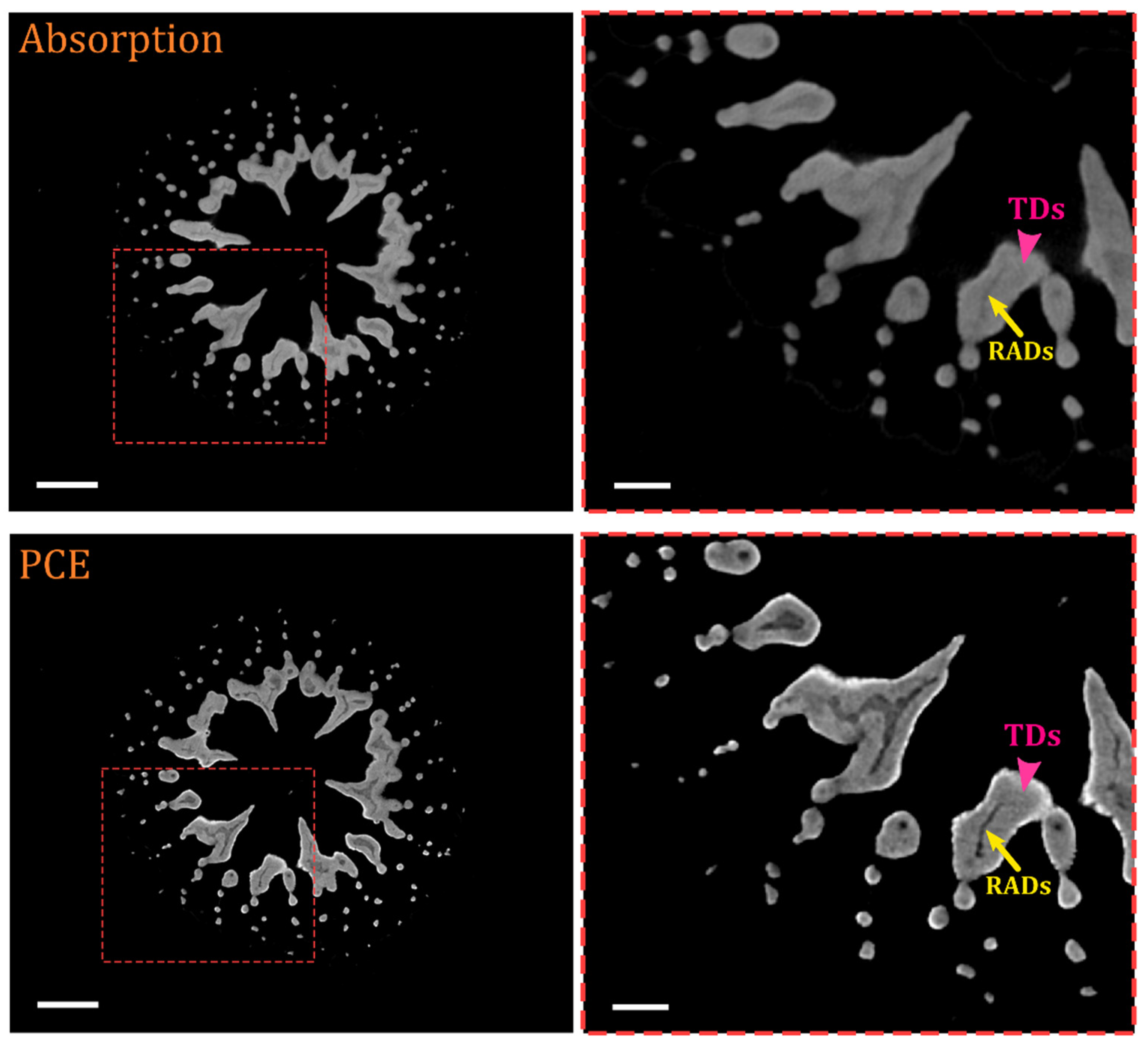
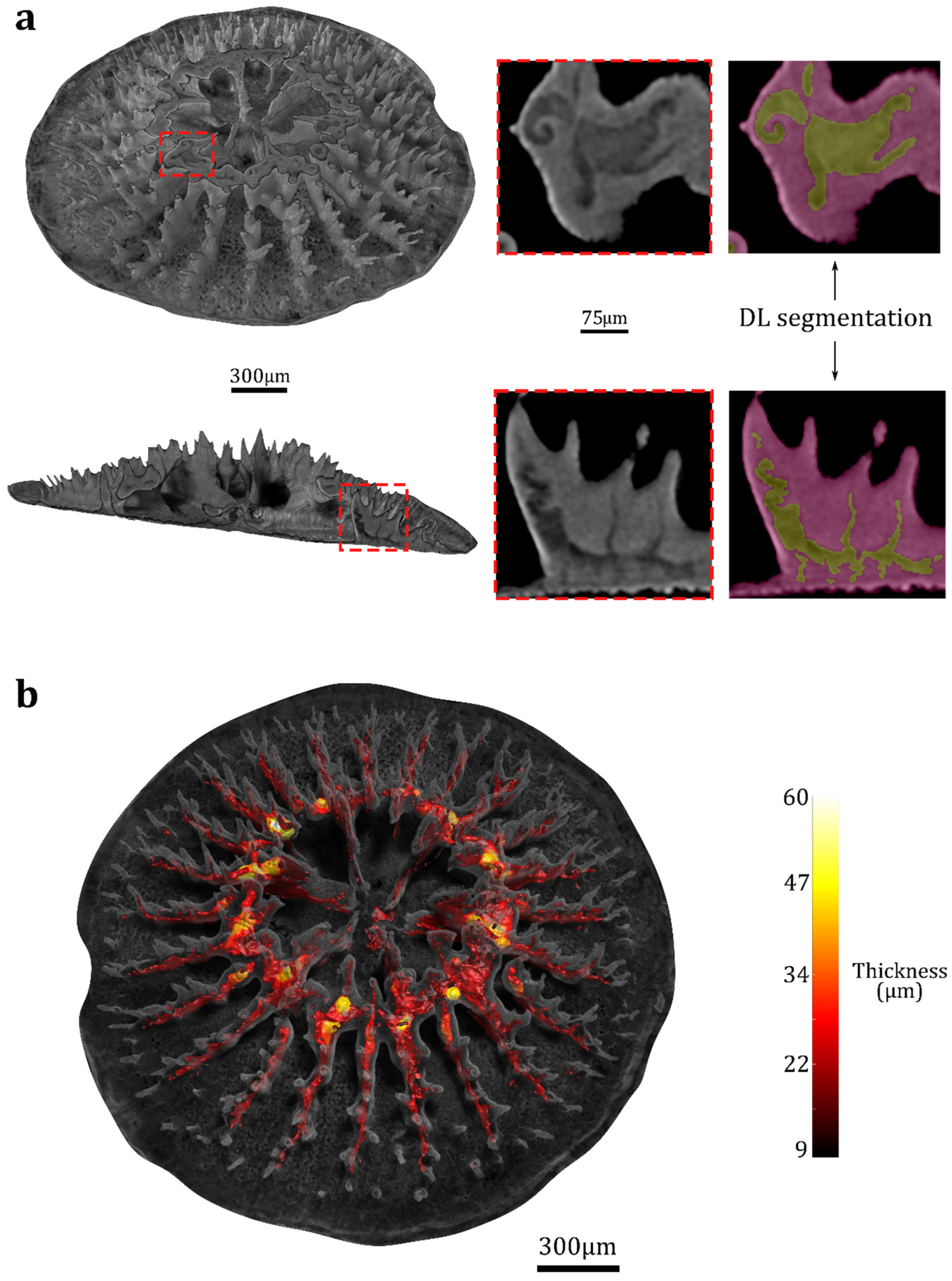
3.1. Detection and Distinction of Coral Skeletal Structures

We reconstructed high-resolution tomography datasets of up to 1000 cross-sectional slices per scanned coral primary polyp, each amounting to a total of 54 GB of data. Each reconstructed image presents the complete form of the original coral skeleton including details of the internal skeletal architecture. In the PCE-CT images, strong differences in contrasts within the skeleton revealed clear internal variations in mineral distribution (Figure 4). Such variations coincide with previous observations of RADs possessing a less compact arrangement of the aragonite aggregates and a higher amount of organics compared to TDs [2,3,8,9,10,11,12,13]. Absorption images further confirm variations in mineral density between skeletal regions, though with blurry edges due to the poor signal. These scans show that RADs are indeed less dense than the surrounding TDs (~20% lower density; Supplemental Figure S2). This clear difference in density allowed us to ascertain that the contrasts observed by PCE-CT correspond to RADs and TDs in all phase contrast enhanced datasets. To allow for volumetric quantification and 3D visualization, image segmentation has to be applied, which requires clear boundaries to be present between different features [55]. The PCE-CT imaging mode appears, therefore, to be perfectly suited for the purpose, as the interfaces between RADs and TDs are accentuated and easy to identify, especially when compared to absorption images (Figure 4).

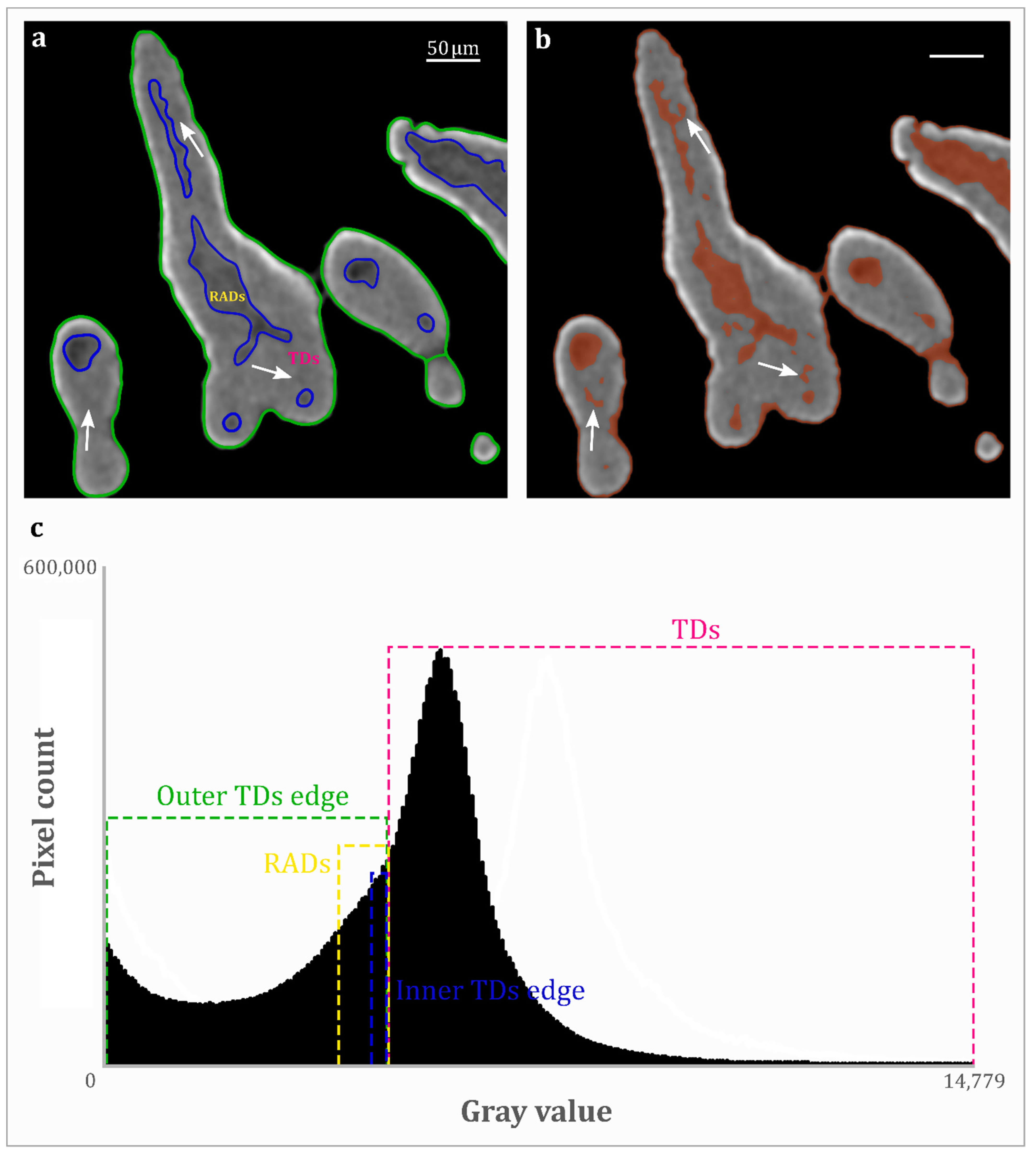
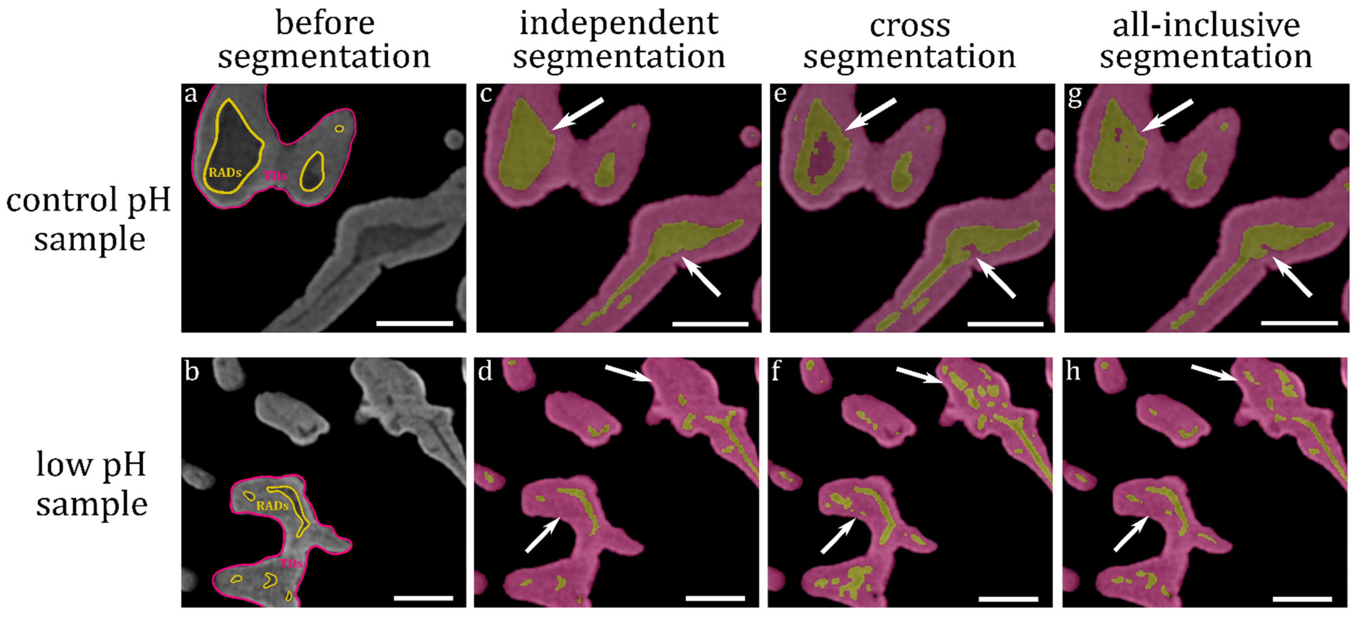
3.2. Segmentation of RADs and TDs

Conventional segmentation methods typically rely on choosing cut-off gray-values and are often based on the voxel intensity histograms. By applying a thresholding, the image can be segmented into the features that are below or above defined threshold values [56]. A gray-value histogram of an example coral skeleton shows that no clear distinction exists in gray-values corresponding TDs and RADs, as there is an overlap between the intensity ranges (for example, see gray-values of the margin of TDs facing the exterior of the skeleton and facing the RADs in Figure 5a,c). Phase-contrast images in fact are edge enhanced, meaning that both the brightest and lowest intensities of the image are found in the margins delineating the edges and internal boundaries of different densities and interfaces in the sample, and meaning that different features of interest may have the same “color”.

Although PCE-CT imaging creates a sharp visual discrimination of RADs and TDs, a simple “binary” threshold applied to this type of image does not yield precise segmentation and reliable distinction between the two skeletal regions, due to the overlap between the intensity range of RADs and the TDs margins. This is shown by the mismatches between the distribution of RADs and TDs as observed in the reconstructed image and the distribution outlined by simple thresholding (Figure 5a,b). Thus, segmentation and ultimately quantification and 3D visualization of RADs and TDs require the use of a more sophisticated technique. Figure 6a depicts results obtained by the automatic segmentation performed using DL networks, which reveals a far better distinction of RADs and TDs within the recruit skeletons. The impressive separation between features becomes evident within the complex shapes of RADs across the skeleton (Video S1), and provides a means for overcoming the limitations imposed by the overlap in gray-values intensity ranges. Such detail-sensitive segmentation of RADs and TDs across an entire stack of slices ultimately allows for accurate volumetric quantification and 3D reproduction of the entire recruit’s skeleton, including fine details of local thickness within RADs (Figure 6b, Video S1).

3.3. Evaluation of the DL-Based Segmentation Performance

Figure 6 and Figure 7c,d show the intricate details made available due to the DL segmentation based on training an independent network (e.g., network A trained and applied on dataset A). Visual inspections of the segmentation outcomes reveal that applying a network optimized on a single tomographic dataset does not always provide a precise segmentation of other datasets (cross segmentation), as demonstrated by small mismatches between the real arrangement of RADs and TDs (as observed in “ground truth” images, Figure 7a,b) and the distribution outlined by the DL segmentation (Figure 7e,f).

Such visual segmentation mismatches for the cross segmentation cases lead to significant differences in the mean per-slice percentage of RADs area over the total area of the skeleton, for both control pH dataset (mean per-slice difference of −1.60% ± 0.07 between the % RADs area/total area obtained with independent segmentation and the one obtained with cross segmentation; Wilcoxon test, W = −20060, p < 0.0001) (red dots compared to green dots in Figure 8a) and for low pH dataset (mean per-slice difference of +7.90% ± 0.38 between the % RADs area/total area obtained with independent segmentation and the one obtained with cross segmentation; Wilcoxon test, W = 13861, p < 0.0001) (purple dots compared to blue dots in Figure 8b). Importantly, however, for the normal pH, the differences are less than 2%, which is impressive given the huge number of slices processed. The generation of such discrepancies may be due to the sensitivity of AI in segmenting images where there are large variations in the shape of the objects of interest between different datasets [51,52,53]. We indeed found substantial variations in the shape of skeletal features among datasets, as indicated by the different skewness values of the distributions of the RADs-TDs shape configurations (Figure 8c,d and Supplemental Figure S3). Curiously though, we did not find a significant correlation between these skewness values and the degree of overestimation or underestimation of the RADs/total skeleton area. This suggests that, on average, DL segmentation does not skew the data and is certainly no less accurate than other segmentation methods.

Notably, differences in the skewness of distributions are particularly evident when comparing datasets across pH conditions. Low pH datasets in fact have a significantly lower mean skewness (5.47 ± 0.48) compared to control pH dataset (mean of 11.13 ± 1.36; Unpaired t test, t = 3.922, p = 0.017) (Figure 8c,d), suggesting an underlying shaping effect of acidic seawater on the RADs-TDs distribution across the recruits skeleton, requiring further in-depth investigation.

Further visual evaluation of the different segmentation outcomes reveals that applying a network trained using all tomographic datasets (named all-inclusive segmentation) provides a much improved segmentation performance compared to the cross segmentation (Figure 7e–h). These observations are supported by the measurements of the mean per-slice percentage of RADs area over the total area of the skeleton (Figure 8a,b). For both control and low pH datasets, the all-inclusive segmentation yielded a significantly better estimation of such percent area than the one produced by the cross segmentation (for the control pH dataset: mean per-slice difference of −0.95% ± 0.10 between the % RADs area/total area obtained with independent segmentation and the one obtained with all-inclusive segmentation, Wilcoxon test, W = −13081, p < 0.0001; for the low pH dataset: mean per-slice difference of +2.65% ± 0.15 between the % RADs area/total area obtained with independent segmentation and the one obtained with all-inclusive segmentation, Wilcoxon test, W = −13651, p < 0.0001)(see red dots compared to yellow dots in Figure 8a and purple dots compared to light blue dots in Figure 8b). These results indicate that variations in the coral geometries themselves increase the variability of shapes encountered by the model during training, which in turn substantially increases the robustness of the DL-based segmentation performance.

4. Discussion

Combining PCE-CT and AI-based image segmentation, we have developed a highly sensitive methodology to obtain quantitative volumetric information about RADs and TDs, the two main skeleton domains of reef-building corals (Figure 6, Video S1). As is the case for many tomographic analyses, image segmentation of the coral is a necessary step for quantitative analytical investigations of the datasets. Our work provides a pipeline that allows to extract the regions corresponding to volumes and densities of interest and to obtain their detailed 3D geometry quantification. Image contrast differences strongly influence the segmentation performance, as they determine how well objects of interests are differentiated by both human and machine vision, thus improving the object perceptual quality [57,58]. In the present study, we show that PCE-CT yields the needed high contrast difference that is essential to visually identify the fine intricate interwoven structures of TDs and RADs within the intact coral skeleton. Indeed, PCE has proven to be a powerful tomographic method in both biomedical research and geological sciences to increase image contrast and enhance image segmentation performance [59].

Although PCE-CT imaging greatly facilitates the visual distinction between RADs and TDs by accentuating their μm-sized boundaries, it introduces difficulties to precisely segment the two skeletal regions using simple segmentation techniques. Specifically, edge enhancement and strong artefacts totally preclude any phase retrieval such as the paganin method [60]. For many datasets, thresholding is the simplest and more common method of segmenting images, which assumes that it is possible to find a single threshold value coinciding with the grayscale intensity of the pixels that correspond to the same structure in the volumetric image [56]. However, accurate image thresholding is only possible in cases where the different features in an image have clearly different peaks in the gray-value histogram. The significant overlap observed between the gray-value ranges of RADs and of the TDs edges makes it impossible to achieve a complete segmentation of the skeletal structures using a simple threshold (Figure 5). It is for this reason that DL algorithms are of great interest, as they may help overcome this difficulty by iteratively learning from data, allowing computers to digitally dissect images through automatic detection and classification of pixels belonging to the structures of interest [61]. In spite of the high complexity of the RADs structure across the recruit skeletons, the automatic segmentation performed by training DL networks delineated and distinguished RADs and TDs with great detail, an essential step on the path for volumetric quantification and visualization (Figure 6 and Video S1). Though computationally intensive, automated image segmentation has been widely reported in recent years for biomedical image segmentation (reviewed in [62]) as well as for mineral characterization [30,31,32,33]. However, up to now, the use of AI for retrieval of biologically interpretable results in the context of coral skeleton morphology has never been reported.

The impressive, robust performance of the DL-based segmentation in identifying and distinguish RADs and TDs across the coral skeleton particularly applies in the case of DL networks optimized for single datasets independently. In contrast, a network that was trained on one specific tomographic dataset yields severe mismatches when applied to segmentation of a different dataset, presumably because it is presented with previously unencountered shape configurations of the target skeletal features (Figure 7 and Figure 8, Supplemental Figure S3). This suggests that the variability in coral geometries must be considered and possibly quantified, when generalizing findings, e.g., TDs or RADs morphologies. Furthermore, this suggests that the performance of AI in segmenting coral skeletal structures is quite sensitive to the large variability of the shape of RADs and TDs that exist among different recruits. Such shape variability is especially evident when comparing control pH recruits to low pH recruits, suggesting a morphologically-altering effect of OA on coral skeletal features that will require further in-depth examination to be deciphered. We speculate that the significant morphological differences tip the ratio between TDs and RADs in the skeletons in such a way that AI needs much more information to fully characterize the effects of OA. Note that the number of regions and slices presented to the DL for training in the normal pH and OA affected recruits was identical. This clearly indicates that normal pH corals are more similar to one another than to the pH affected corals.

Indeed, varying appearance of target features poses a great challenge in image segmentation (reviewed in [54]). For example in medical research, there can be wide differences between different medical images that affect the adaptability of DL network models during segmentation [62,63]. This is mainly due to the heterogeneous appearance of target organs for segmentation, which may vary hugely in size, shape and location from one patient to the other [64]. Another aspect that may restrict the performance of DL-based image segmentation is the limited diversity of data available to train a network [54,62,63]. Here, we show that widening the spectrum of possible appearances of the target skeletal features to be recognized using AI across multiple datasets considerably improves the DL-based segmentation performance (Figure 7 and Figure 8). This showcases the power of AI when fed with diverse training data, and the potential of application across multiple tomographic datasets.

A commonly adopted method to generate new samples and increase the size of the training datasets is data augmentation, which is the application of a set of image transformations (e.g., rotation or flipping) to the dataset [65]. In this way, previously unencountered target features can potentially be approximated by the network. However, this method also adds sources of error and variability to the general methodological framework, as so far there is no strict consensus on which transformation to introduce and generally the transformation parameters are inconstantly chosen [54]. In this regard, we aim at improving the performance and generalizability of DL models across diverse coral datasets by collecting a larger diverse array of coral tomography data. If such datasets are made publicly available through, for example, open-access online databases, they will form a source of data that can be used to train robust, efficient, and generalizable DL models for use in coral research. It should be noted that image processing and segmentation of entire coral polyps with resolutions of ~2 µm and, in particular, using DL networks require very large computation memory and power, for which high-performance workstations may not be ubiquitously available. Yet, providing tools to help researchers analyze and utilize such data is essential, thus forming a data-collection-analysis feedback loop. Our work presented here is a first step on this ambitious path.

5. Conclusions

To the best of our knowledge, this is the first study that applied AI approaches to investigate the internal 3D geometry of RADs and TDs in coral skeletons based on high-sensitivity, non-destructive PCE-CT data. The approach presented here opens the possibility of using AI to reconstruct and quantitatively analyze the internal skeletal network of reef-building corals. In particular, such technology has the potential to improve ecological monitoring programs, by assessing coral skeletal anatomy and providing morphological descriptors in order to taxonomize hard corals to genus and species levels. In addition, it can expand our knowledge on coral biomineralization by providing a means of characterizing the microscale interfaces within the different coral skeletal regions. Lastly, such a tool allows us to study the dynamics of coral skeletal formation under a variety of environmental conditions, including predicted OA scenarios.

In the last decades we witnessed a significant decline in coral reefs all over the world, and as global climate changes are becoming more severe, the need to protect coral reefs is becoming urgent. Hence, applying materials science contrast-enhanced methods to structural research in corals would be of great benefit for the development of highly targeted restoration strategies, as it would critically expand our knowledge on the effects of environmental change on coral skeleton development.

References

1. Brahmi, C.; Domart-Coulon, I.; Rougée, L.; Pyle, D.G.; Stolarski, J.; Mahoney, J.J.; Richmond, R.H.; Ostrander, G.K.; Meibom, A. Pulsed 86Sr-labeling and NanoSIMS imaging to study coral biomineralization at ultra-structural length scales. Coral Reefs 2012, 31, 741–752. [Google Scholar] [CrossRef] [Green Version]
2. Cuif, J.-P.; Dauphin, Y. The two-step mode of growth in the scleractinian coral skeletons from the micrometre to the overall scale. J. Struct. Biol. 2005, 150, 319–331. [Google Scholar] [CrossRef] [PubMed]
3. Stolarski, J. Three-dimensional micro-and nanostructural characteristics of the scleractinian coral skeleton: A biocalcification proxy. Acta Palaeontol. Pol. 2003, 48, 4. [Google Scholar]
4. Meibom, A.; Cuif, J.-P.; Hillion, F.; Constantz, B.R.; Juillet-Leclerc, A.; Dauphin, Y.; Watanabe, T.; Dunbar, R.B. Distribution of magnesium in coral skeleton: MG microdistribution in coral. Geophys. Res. Lett. 2004, 31. [Google Scholar] [CrossRef]
5. Von Euw, S.; Zhang, Q.; Manichev, V.; Murali, N.; Gross, J.; Feldman, L.C.; Gustafsson, T.; Flach, C.; Mendelsohn, R.; Falkowski, P.G. Biological control of aragonite formation in stony corals. Science 2017, 356, 933–938. [Google Scholar] [CrossRef] [Green Version]
6. Mass, T.; Giuffre, A.J.; Sun, C.-Y.; Stifler, C.A.; Frazier, M.J.; Neder, M.; Tamura, N.; Stan, C.V.; Marcus, M.A.; Gilbert, P.U.P.A. Amorphous calcium carbonate particles form coral skeletons. Proc. Natl. Acad. Sci. USA 2017, 114, E7670–E7678. [Google Scholar] [CrossRef] [PubMed] [Green Version]
7. Neder, M.; Laissue, P.P.; Akiva, A.; Akkaynak, D.; Albéric, M.; Spaeker, O.; Politi, Y.; Pinkas, I.; Mass, T. Mineral formation in the primary polyps of pocilloporoid corals. Acta Biomater. 2019, 96, 631–645. [Google Scholar] [CrossRef]
8. Cuif, J.-P.; Dauphin, Y. Microstructural and physico-chemical characterization of ‘centers of calcification’ in septa of some Recent scleractinian corals. Paläontol. Z. 1998, 72, 257–269. [Google Scholar] [CrossRef]
9. Frankowiak, K.; Mazur, M.; Gothmann, A.M.; Stolarski, J. Diagenetic alteration of triassic coral from the aragonite konservat-lagerstatte in alakir cay, turkey: Implications for geochemical measurements. Palaios 2013, 28, 333–342. [Google Scholar] [CrossRef]
10. Mass, T.; Drake, J.L.; Peters, E.C.; Jiang, W.; Falkowski, P.G. Immunolocalization of skeletal matrix proteins in tissue and mineral of the coral Stylophora pistillata. Proc. Natl. Acad. Sci. USA 2014, 111, 12728–12733. [Google Scholar] [CrossRef] [Green Version]
11. Sugiura, M.; Yasumoto, K.; Iijima, M.; Oaki, Y.; Imai, H. Morphological study of fibrous aragonite in the skeletal framework of a stony coral. CrystEng. Comm. 2021, 23, 3693–3700. [Google Scholar] [CrossRef]
12. Benzerara, K.; Menguy, N.; Obst, M.; Stolarski, J.; Mazur, M.; Tylisczak, T.; Brown, G.E.; Meibom, A. Study of the crystallographic architecture of corals at the nanoscale by scanning transmission X-ray microscopy and transmission electron microscopy. Ultramicroscopy 2011, 111, 1268–1275. [Google Scholar] [CrossRef] [PubMed]
13. Brahmi, C.; Meibom, A.; Smith, D.C.; Stolarski, J.; Auzoux-Bordenave, S.; Nouet, J.; Doumenc, D.; Djediat, C.; Domart-Coulon, I. Skeletal growth, ultrastructure and composition of the azooxanthellate scleractinian coral Balanophyllia regia. Coral Reefs 2010, 29, 175–189. [Google Scholar] [CrossRef]
14. Cohen, A.; Holcomb, M. Why Corals Care About Ocean Acidification: Uncovering the Mechanism. Oceanograpgy 2009, 22, 118–127. [Google Scholar] [CrossRef]
15. Erez, J.; Reynaud, S.; Silverman, J.; Schneider, K.; Allemand, D. Coral Calcification Under Ocean Acidification and Global Change. In Coral Reefs: An Ecosystem in Transition; Dubinsky, Z., Stambler, N., Eds.; Springer Netherlands: Dordrecht, The Netherlands, 2011; pp. 151–176. ISBN 978-94-007-0113-7. [Google Scholar]
16. Kleypas, J.A.; Langdon, C. Coral reefs and changing seawater carbonate chemistry. In Coastal and Estuarine Studies; Phinney, J.T., Hoegh-Guldberg, O., Kleypas, J., Skirving, W., Strong, A., Eds.; American Geophysical Union: Washington, DC, USA, 2006; Volume 61, pp. 73–110. ISBN 978-0-87590-359-0. [Google Scholar]
17. Marubini, F.; Ferrier–Pages, C.; Cuif, J. Suppression of skeletal growth in scleractinian corals by decreasing ambient carbonate-ion concentration: A cross-family comparison. Proc. R. Soc. Lond. B 2003, 270, 179–184. [Google Scholar] [CrossRef] [Green Version]
18. Mollica, N.R.; Guo, W.; Cohen, A.L.; Huang, K.-F.; Foster, G.L.; Donald, H.K.; Solow, A.R. Ocean acidification affects coral growth by reducing skeletal density. Proc. Natl. Acad. Sci. USA 2018, 115, 1754–1759. [Google Scholar] [CrossRef] [Green Version]
19. Scucchia, F.; Malik, A.; Zaslansky, P.; Putnam, H.M.; Mass, T. Combined responses of primary coral polyps and their algal endosymbionts to decreasing seawater pH. Proc. R. Soc. B 2021, 288, 20210328. [Google Scholar] [CrossRef]
20. Cohen, A.L.; McCorkle, D.C.; de Putron, S.; Gaetani, G.A.; Rose, K.A. Morphological and compositional changes in the skeletons of new coral recruits reared in acidified seawater: Insights into the biomineralization response to ocean acidification. Geochem. Geophys. Geosyst. 2009, 10. [Google Scholar] [CrossRef] [Green Version]
21. Nothdurft, L.D.; Webb, G.E. Microstructure of Common Reef-Building Coral Genera Acropora, Pocillopora, Goniastrea and Porites: Constraints on Spatial Resolution in Geochemical Sampling. Facies 2007, 53, 1–26. [Google Scholar] [CrossRef]
22. Cnudde, V.; Boone, M.N. High-resolution X-ray computed tomography in geosciences: A review of the current technology and applications. Earth-Sci. Rev. 2013, 123, 1–17. [Google Scholar] [CrossRef] [Green Version]
23. Kyle, J.R.; Ketcham, R.A. Application of high resolution X-ray computed tomography to mineral deposit origin, evaluation, and processing. Ore Geol. Rev. 2015, 65, 821–839. [Google Scholar] [CrossRef]
24. Cloetens, P.; Pateyron-Salomé, M.; Buffière, J.Y.; Peix, G.; Baruchel, J.; Peyrin, F.; Schlenker, M. Observation of microstructure and damage in materials by phase sensitive radiography and tomography. J. Appl. Phys. 1997, 81, 5878–5886. [Google Scholar] [CrossRef]
25. Baruchel, J. X-ray Tomography in Material Science; Hermes Science: Paris, France, 2000; ISBN 978-2-7462-0115-6. [Google Scholar]
26. De Albuquerque, V.H.C.; Cortez, P.C.; de Alexandria, A.R.; Tavares, J.M.R.S. A new solution for automatic microstructures analysis from images based on a backpropagation artificial neural network. Nondestruct. Test. Eval. 2008, 23, 273–283. [Google Scholar] [CrossRef]
27. De Albuquerque, V.H.C.; Tavares, J.M.R.S.; Durão, L.M.P. Evaluation of Delamination Damage on Composite Plates using an Artificial Neural Network for the Radiographic Image Analysis. J. Compos. Mater. 2010, 44, 1139–1159. [Google Scholar] [CrossRef]
28. Iglesias, J.C.Á.; Santos, R.B.M.; Paciornik, S. Deep learning discrimination of quartz and resin in optical microscopy images of minerals. Miner. Eng. 2019, 138, 79–85. [Google Scholar] [CrossRef]
29. Buyya, R.; Calheiros, R.N.; Dastjerdi, A.V. (Eds.) Big Data: Principles and Paradigms; Elsevier/Morgan Kaufmann: Cambridge, MA, USA, 2016; ISBN 978-0-12-805394-2. [Google Scholar]
30. Chauhan, S.; Rühaak, W.; Anbergen, H.; Kabdenov, A.; Freise, M.; Wille, T.; Sass, I. Phase segmentation of X-ray computer tomography rock images usingmachine learning techniques: An accuracy and performancestudy. Solid Earth 2016, 7, 1125–1139. [Google Scholar] [CrossRef] [Green Version]
31. Chauhan, S.; Rühaak, W.; Khan, F.; Enzmann, F.; Mielke, P.; Kersten, M.; Sass, I. Processing of rock core microtomography images: Using seven different machine learning algorithms. Comput. Geosci. 2016, 86, 120–128. [Google Scholar] [CrossRef]
32. Varfolomeev, I.; Yakimchuk, I.; Safonov, I. An Application of Deep Neural Networks for Segmentation of Microtomographic Images of Rock Samples. Computers 2019, 8, 72. [Google Scholar] [CrossRef] [Green Version]
33. Wang, Y.; Lin, C.L.; Miller, J.D. Improved 3D image segmentation for X-ray tomographic analysis of packed particle beds. Miner. Eng. 2015, 83, 185–191. [Google Scholar] [CrossRef]
34. Van Vuuren, D.P.; Edmonds, J.; Kainuma, M.; Riahi, K.; Thomson, A.; Hibbard, K.; Hurtt, G.C.; Kram, T.; Krey, V.; Lamarque, J.-F.; et al. The representative concentration pathways: An overview. Clim. Chang. 2011, 109, 5–31. [Google Scholar] [CrossRef]
35. Pörtner, H.-O.; Roberts, D.C.; Masson-Delmotte, V.; Zhai, P.; Tignor, M.; Poloczanska, E.; Mintenbeck, K.; Alegría, A.; Nicolai, M.; Okem, A.; et al. (Eds.) Special Report on the Ocean and Cryosphere in a Changing Climate; IPCC: Geneva, Switzerland, 2019. [Google Scholar]
36. Goodbody-Gringley, G. Diel Planulation by the Brooding Coral Favia Fragum (Esper, 1797). J. Exp. Mar. Biol. Ecol. 2010, 389, 70–74. [Google Scholar] [CrossRef]
37. Goodbody-Gringley, G.; Wong, K.H.; Becker, D.M.; Glennon, K.; de Putron, S.J. Reproductive Ecology and Early Life History Traits of the Brooding Coral, Porites astreoides, from Shallow to Mesophotic Zones. Coral Reefs 2018, 37, 483–494. [Google Scholar] [CrossRef]
38. Pierrot, D.; Lewis, E.; Wallace, D.W.R. MS Excel Program Developed for CO2 System Calculations; ORNL/CDIAC-105a; Carbon Dioxide Information Analysis Center, Oak Ridge National Laboratory, US Department of Energy: Oak Ridge, TN, USA, 2006; Volume 10.
39. Mehrbach, C.; Culberson, C.H.; Hawley, J.E.; Pytkowicx, R.M. Measurement of the apparent dissociation constants of carbonic acid in seawater at atmospheric pressure 1. Limnol. Oceanogr. 1973, 18, 897–907. [Google Scholar] [CrossRef]
40. Dickson, A.G.; Millero, F.J. A comparison of the equilibrium constants for the dissociation of carbonic acid in seawater media. Deep. Sea Res. Part A Oceanogr. Res. Pap. 1987, 34, 1733–1743. [Google Scholar] [CrossRef]
41. Görner, W.; Hentschel, M.P.; Müller, B.R.; Riesemeier, H.; Krumrey, M.; Ulm, G.; Diete, W.; Klein, U.; Frahm, R. BAMline: The first hard X-ray beamline at BESSY II. Nucl. Instrum. Methods Phys. Res. Sect. A 2001, 467–468, 703–706. [Google Scholar] [CrossRef]
42. Rack, A.; Zabler, S.; Müller, B.R.; Riesemeier, H.; Weidemann, G.; Lange, A.; Goebbels, J.; Hentschel, M.; Görner, W. High resolution synchrotron-based radiography and tomography using hard X-rays at the BAMline (BESSY II). Nucl. Instrum. Methods Phys. Res. Sect. A 2008, 586, 327–344. [Google Scholar] [CrossRef]
43. Zaslansky, P.; Fratzl, P.; Rack, A.; Wu, M.-K.; Wesselink, P.R.; Shemesh, H. Identification of root filling interfaces by microscopy and tomography methods: Microtomography and microscopy observations of root fillings. Int. Endod. J. 2011, 44, 395–401. [Google Scholar] [CrossRef]
44. Reznikov, N.; Buss, D.J.; Provencher, B.; McKee, M.D.; Piché, N. Deep learning for 3D imaging and image analysis in biomineralization research. J. Struct. Biol. 2020, 212, 107598. [Google Scholar] [CrossRef]
45. Schindelin, J.; Arganda-Carreras, I.; Frise, E.; Kaynig, V.; Longair, M.; Pietzsch, T.; Preibisch, S.; Rueden, C.; Saalfeld, S.; Schmid, B.; et al. Fiji: An open-source platform for biological-image analysis. Nat. Methods 2012, 9, 676–682. [Google Scholar] [CrossRef] [Green Version]
46. Makovetsky, R.; Piche, N.; Marsh, M. Dragonfly as a Platform for Easy Image-based Deep Learning Applications. Microsc. Microanal. 2018, 24, 532–533. [Google Scholar] [CrossRef] [Green Version]
47. Tan, Y. Applications. In Gpu-Based Parallel Implementation of Swarm Intelligence Algorithms; Elsevier: Amsterdam, The Netherlands, 2016; pp. 167–177. ISBN 978-0-12-809362-7. [Google Scholar]
48. Ronneberger, O.; Fischer, P.; Brox, T. U-Net: Convolutional Networks for Biomedical Image Segmentation. In Medical Image Computing and Computer-Assisted Intervention—MICCAI 2015; Navab, N., Hornegger, J., Wells, W.M., Frangi, A.F., Eds.; Lecture Notes in Computer Science; Springer International Publishing: Cham, Switzerland, 2015; Volume 9351, pp. 234–241. ISBN 978-3-319-24573-7. [Google Scholar]
49. Hamwood, J.; Alonso-Caneiro, D.; Read, S.A.; Vincent, S.J.; Collins, M.J. Effect of patch size and network architecture on a convolutional neural network approach for automatic segmentation of OCT retinal layers. Biomed. Opt. Express 2018, 9, 3049. [Google Scholar] [CrossRef] [Green Version]
50. Sudre, C.H.; Li, W.; Vercauteren, T.; Ourselin, S.; Jorge Cardoso, M. Generalised Dice Overlap as a Deep Learning Loss Function for Highly Unbalanced Segmentations. In Deep Learning in Medical Image Analysis and Multimodal Learning for Clinical Decision Support; Cardoso, M.J., Arbel, T., Carneiro, G., Syeda-Mahmood, T., Tavares, J.M.R.S., Moradi, M., Bradley, A., Greenspan, H., Papa, J.P., Madabhushi, A., et al., Eds.; Lecture Notes in Computer Science; Springer International Publishing: Cham, Switzerland, 2017; Volume 10553, pp. 240–248. ISBN 978-3-319-67557-2. [Google Scholar]
51. Khalifa, F.; El-Baz, A.; Gimel’farb, G.; Ouseph, R.; El-Ghar, M.A. Shape-Appearance Guided Level-Set Deformable Model for Image Segmentation. In Proceedings of the 2010 20th International Conference on Pattern Recognition, Istanbul, Turkey, 23–26 August 2010; pp. 4581–4584. [Google Scholar]
52. El-Baz, A.; Gimel’farb, G. Robust image segmentation using learned priors. In Proceedings of the 2009 IEEE 12th International Conference on Computer Vision, Kyoto, Japan, 29 September–2 October 2009; pp. 857–864. [Google Scholar]
53. Chen, F.; Yu, H.; Hu, R.; Zeng, X. Deep Learning Shape Priors for Object Segmentation. In Proceedings of the 2013 IEEE Conference on Computer Vision and Pattern Recognition, Portland, OR, USA, 23–28 June 2013; pp. 1870–1877. [Google Scholar]
54. Renard, F.; Guedria, S.; Palma, N.D.; Vuillerme, N. Variability and reproducibility in deep learning for medical image segmentation. Sci. Rep. 2020, 10, 13724. [Google Scholar] [CrossRef] [PubMed]
55. Sharon, E.; Brandt, A.; Basri, R. Segmentation and boundary detection using multiscale intensity measurements. In Proceedings of the 2001 IEEE Computer Society Conference on Computer Vision and Pattern Recognition, Kauai, HI, USA, 8–14 December 2001; Volume 1. [Google Scholar]
56. Guntoro, P.I.; Ghorbani, Y.; Koch, P.-H.; Rosenkranz, J. X-ray Microcomputed Tomography (µCT) for Mineral Characterization: A Review of Data Analysis Methods. Minerals 2019, 9, 183. [Google Scholar] [CrossRef] [Green Version]
57. Campos, G.F.C.; Mastelini, S.M.; Aguiar, G.J.; Mantovani, R.G.; de Melo, L.F.; Barbon, S. Machine learning hyperparameter selection for Contrast Limited Adaptive Histogram Equalization. J. Image Video Proc. 2019, 2019, 59. [Google Scholar] [CrossRef] [Green Version]
58. Saleem, A.; Beghdadi, A.; Boashash, B. Image fusion-based contrast enhancement. J. Image Video Proc. 2012, 2012, 10. [Google Scholar] [CrossRef] [Green Version]
59. Withers, P.J.; Bouman, C.; Carmignato, S.; Cnudde, V.; Grimaldi, D.; Hagen, C.K.; Maire, E.; Manley, M.; Du Plessis, A.; Stock, S.R. X-ray computed tomography. Nat. Rev. Methods Primers 2021, 1, 18. [Google Scholar] [CrossRef]
60. Paganin, D.; Mayo, S.C.; Gureyev, T.E.; Miller, P.R.; Wilkins, S.W. Simultaneous phase and amplitude extraction from a single defocused image of a homogeneous object. J. Microsc. 2002, 206, 33–40. [Google Scholar] [CrossRef]
61. LeCun, Y.; Bengio, Y.; Hinton, G. Deep learning. Nature 2015, 521, 436–444. [Google Scholar] [CrossRef]
62. Liu, X.; Song, L.; Liu, S.; Zhang, Y. A Review of Deep-Learning-Based Medical Image Segmentation Methods. Sustainability 2021, 13, 1224. [Google Scholar] [CrossRef]
63. Hesamian, M.H.; Jia, W.; He, X.; Kennedy, P. Deep Learning Techniques for Medical Image Segmentation: Achievements and Challenges. J. Digit. Imag. 2019, 32, 582–596. [Google Scholar] [CrossRef] [Green Version]
64. Kamnitsas, K.; Ledig, C.; Newcombe, V.F.J.; Simpson, J.P.; Kane, A.D.; Menon, D.K.; Rueckert, D.; Glocker, B. Efficient multi-scale 3D CNN with fully connected CRF for accurate brain lesion segmentation. Med. Image Anal. 2017, 36, 61–78. [Google Scholar] [CrossRef] [PubMed]
65. Shorten, C.; Khoshgoftaar, T.M. A survey on Image Data Augmentation for Deep Learning. J. Big Data 2019, 6, 60. [Google Scholar] [CrossRef]
Figure 1. Workflow for acquisition and processing of tomographic datasets of coral recruit skeletons. (a) X-ray projections are acquired from different angles of the skeleton with incremental rotation (0° to 180°); (b) following normalization (gray star = additional details are shown in Figure 2), tomographic cross-sectional slices are reconstructed; (c) cross-sectional slices are stacked and processed into 3D views of the recruit skeletons; (d) AI-based segmentation and classification are performed so that the features of interest can be analyzed and visualized in 3D. An example distribution of RAD thicknesses is shown.
Jmse 10 00391 g001
Figure 2. Example X-ray µCT radiographs of a recruit skeleton as obtained on the beamline (left) and after normalization (right). Radiographs were background-corrected by normalization with empty beam (flat-field) images and by the subtraction of dark-current images. The dark silhouette of the coral is seen to be suspended within a faint halo of epoxy resin, visible in the normalized (right) image.
Jmse 10 00391 g002
Figure 3. Overview of the DL (deep-learning-based) image segmentation process. (a) Example tomographic cross-sectional slices across the skeleton of a primary polyp before segmentation, revealing RADs (dark gray areas, yellow arrows) enclosed within TDs (light gray areas, pink arrowheads). (b,c) Manually delineated RADs (b; marked in yellow) and TDs (c; marked in pink) defined in a confined region within the training dataset. (d) Complete region manually delineated as training dataset, showing all three features (RADs in yellow, TDs in pink, and air spaces in green). (e) Result of the complete dataset processed by automatic DL-based segmentation. The AI network was applied to all slices within the stack, and it has automatically successfully distinguished RADs (yellow) and TDs (pink). Scale bars: 300 µm.
Jmse 10 00391 g003
Figure 4. Typical coral skeleton details observed in cross-sectional tomography slices and comparison between absorption and PCE imaging modes. Differences in X-ray absorption within the skeleton reveal variations in both mineral distribution and density between RADs (darker regions correspond to lower density) and TDs (lighter regions, higher density); the red marked insets are shown on the right. Strongly defined boundaries can be observed between RADs and TDs in slices from PCE-CT datasets, whereas absorption images provide a blurry, poorly distinguishable separation between the two skeletal regions. Scale bars: 300 µm (left images), 100 µm (right images).
Jmse 10 00391 g004
Figure 5. Slices and typical histogram of gray-values in PCE image and quality of non-DL-based image segmentation. (a) Close-up of the skeleton, showing RADs (dark gray areas), TDs (light gray areas), and delineating the outer and inner edges of TDs (green and pink lines, respectively). (b) Result of a simple threshold applied to segment RADs (RADs segmented by the thresholding method are colored in red). Note that, compared to their actual shape in the ground truth image (a), RADs are not precisely segmented (see arrows for example mismatch, where TDs regions are classified as RADs) and they are not distinguished from the outer edge of TDs, which are also thresholded as RADs by this method. (c) Gray-value histogram for an example tomographic stack of an imaged coral skeleton. The gray-value ranges for all regions depicted in (a) are highlighted in different colors. Note the overlap between the gray-value ranges of RADs and of the inner/outer edges of TDs, which makes it impossible to reliably segment these regions by simple threshold, as demonstrated in (b).
Jmse 10 00391 g005
Figure 6. Deep-Learning-based image segmentation and quantitative 3D reproduction of segmented RADs and TDs. (a) Two example 3D renderings of a primary polyp skeleton virtually sliced in the transverse plane (upper row) and in the longitudinal plane (bottom row). Red dotted lines show enlargements of the sliced skeleton that have been segmented using DL (segmented TDs and RADs are colored in pink and yellow, respectively). DL, Deep Learning. (b) Segmentation of RADs and TDs across the entire stack of slices allows 3D separation of features and quantification, including details of local thickness (µm).
Jmse 10 00391 g006
Figure 7. Evaluation of the DL-based segmentation performance. (a,b) Details of the skeletal structures in representative coral recruits from the control and low pH conditions before applying the DL-based segmentation (ground truth images). RADs and TDs in example areas have been manually delineated in yellow and pink, respectively. (c,d) Segmentation of RADs and TDs based on training a network independently per each single dataset. Specifically, (c) shows the outcome of the segmentation of network A trained and applied on dataset A (a representative control pH sample), whereas (d) shows the outcome of the segmentation of network X trained and applied on dataset X (a representative low pH sample). (e) Segmentation obtained by employing a DL network that was trained using dataset B (another representative control pH sample) and applied to dataset A. The white arrows point to mismatches in the segmentation as compared to the more accurate segmentation in (c). Note how RAD regions have been segmented as TDs. (f) Segmentation obtained by training the DL network on dataset A and using it to segment dataset X. The white arrows point to mismatches in the segmentation as compared to the correct segmentation in (d). (g,h) Segmentation obtained by employing a DL network that was trained using all tomographic datasets (all 6 datasets from both control and pH conditions). White arrows identify example points where different segmentation is seen in (g) as compared to (e), and the better segmentation in (h) as compared to (f). Scale bars: 100 µm.
Jmse 10 00391 g007
Figure 8. Evaluation of the DL-based segmentation performance based on the per-slice estimation of the area of the coral skeletal features and skewness of the distributions of the RADs-TDs shape configuration across samples. (a,b) Measured per-slice area of RADs over the total area of the skeleton (RADs + TDs) estimated using independent, cross, and all-inclusive segmentations (as shown in Figure 7) in the case of a control pH sample (a) and a low pH sample (b). The slice number indicates the progression through the recruit’s skeleton going from the base to the top, as illustrated by the coral skeletons on the right side of the graphs. Note how, for both control and low pH datasets, the per-slice area of the RADs obtained with all-inclusive segmentation gets closer to the value obtained with independent segmentation (red dots versus yellow dots and purple dots versus light blue dots, respectively) compared to the per-slice area obtained with cross segmentation (red dots versus green dots and purple dots versus blue dots, respectively). (c,d) Skewness of the distributions of the per-slice RADs-TDs shape configuration in control pH (c) and low pH (d) samples (see also Supplemental Figure S3). The ratio of the RADs perimeter/area over the TDs perimeter/area (“C”) was computed as an estimate of the relative shape of the skeletal features across the recruit skeletons. The skewness values are used as a metric to evaluate the degree of the RADs-TDs shape variation across datasets.
Jmse 10 00391 g008
Publisher’s Note: MDPI stays neutral with regard to jurisdictional claims in published maps and institutional affiliations.