Shoaling Wave Shape Estimates from Field Observations and Derived Bedload Sediment Rates

Abstract

The shoaling transformation from generally linear deep-water waves to asymmetric shallow-water waves modifies wave shapes and causes near-bed orbital velocities to become asymmetrical, contributing to net sediment transport. In this work, we used two methods to estimate the asymmetric wave shape from data at three sites. The first method converted wave measurements made at the surface to idealized near-bottom wave-orbital velocities using a set of empirical equations: the “parameterized” waveforms. The second method involved direct measurements of velocities and pressure made near the seabed: the “direct” waveforms. Estimates from the two methods were well correlated at all three sites (Pearson’s correlation coefficient greater than 0.85). Both methods were used to drive bedload-transport calculations that accounted for asymmetric waves, and the results were compared with a traditional excess-stress formulation and field estimates of bedload transport derived from ripple migration rates based on sonar imagery. The cumulative bedload transport from the parameterized waveform was 25% greater than the direct waveform, mainly because the parameterized waveform did not account for negative skewness. Calculated transport rates were comparable to rates estimated from ripple migration except during the largest event, when calculated rates were as much as 100 times greater, which occurred during high period waves.

1. Introduction

Waves propagating towards the coast undergo transformations from their sinusoidal wave shape in deep water to non-linear wave shape in shallow water. “Skewed”, as used here, describes wave shapes, bottom-orbital velocities, and sediment transport generated by waves that cannot be adequately represented by linear (Airy) wave theory (e.g., [1]). The fundamental equations for continuity of mass and momentum used as the starting point for most wave theories are linear, but the surface boundary conditions are not. Linear wave theory neglects the non-linear components by assuming that the ratio of wave height/wavelength (wave steepness) is small. As waves shoal and steepen, this assumption no longer holds, and non-linear equations are needed to accurately represent the waves [1]. Outside the surf zone, this shoaling transformation causes the near-bottom wave orbital velocity to differ between the wave crest and trough cycles, referred to as velocity skewness [2]. As waves propagate further into the surf zone, the differential duration in crest and trough half cycles can lead to a differential acceleration in each half cycle, referred to as acceleration asymmetry [3].

The effect of shoaling waves on resulting sediment dynamics has been quantified in various studies. In previous flume experiments [4,5,6], skewed waves led to onshore sediment transport near the bed. Under mild wave conditions, velocity skewness has been found to be the main driver of onshore sediment transport, generating onshore sandbar migration [7,8,9]. The combined effect of different asymmetric wave shapes in the presence of currents acting against the direction of waves and showed that under decreasing skewed-asymmetric wave shapes, net offshore sediment transport increased [10]. Onshore sediment transport has been also related to ripple migration associated with velocity skewness in several field observations [11,12,13]. Other than flume and field data, numerical models [14,15,16] have shown that acceleration asymmetry caused high onshore sediment transport and contributed towards beach recovery. In addition, process-based morphodynamic modeling studies have shown the impact of wave-induced cross-shore sediment transport that caused inlet closure during weak inlet current conditions [17,18,19]. In another study [20], a numerical model in an idealized inlet domain that accounted for asymmetric waves showed that larger waves contributed to the migration and growth of shoals on ebb-tidal deltas. Using a realistic domain [21], it was shown that the skewness of the waves was responsible for the enhancement of sediment transport into the inlet and the evolution of the ebb-tidal delta during storm conditions. Recent modeling [22,23,24,25,26] studies have shown the importance of wave-driven transport under combined action during wave-current interaction.

These studies highlight the importance of estimating the asymmetric waveforms that affect nearshore sediment transport. Other efforts [27,28] emphasized that understanding wave-driven sediment transport is fundamental to the improvement of morphodynamic models. In the presence of waves, morphodynamic models need to account for both suspended and bedload transport. Of the two modes of sediment transport, bedload transport is most affected by near-bottom wave orbital wave motions [29], thus necessitating the need to estimate asymmetric waveforms in modeling frameworks. Asymmetric waveforms can be computed by wave-resolving models [30,31], but these models are computationally expensive and impractical for regional-scale morphodynamic models. One approach to estimating asymmetric waveforms used a statistical method [32] that applied a genetic algorithm to obtain velocity skewness based on field observations made under shoaling and breaking wave conditions. Another approach to quantify asymmetry from shoaling waves is to use the bulk wave statistics and local depth [33,34]. The approach mentioned in [34] would be referred to as Ruessink’s method. A recent study [35] compared the modified version of the approach mentioned in [33] to Ruessink’s method [34] to simulate long-term morphodynamic change. They [35] found that Ruessink’s method provided a better representation of wave and near-bed orbital velocities, required less calibration and, therefore, resulted in more realistic morphodynamic predictions. A modification to Ruessink’s approach was used in a study [36] to accelerate the model calculations to capture the effects of nourishment on cross-shore bedload fluxes at different locations on an idealized planar beach. Ruessink’s parameterization also showed a good skill predicting shoreward evolution of wave skewness and asymmetry under high-energy waves ($H_s~ 2 \mathrm{m}$) during offshore sandbar migration events [37].

In the present work, we analyzed the efficacy of the widely used Ruessink’s parameterization by taking observations from three sites located outside the surf zone. At these sites, conditions (including depth and wave characteristics) only generate velocity skewness in the waveform shape; acceleration skewness becomes more important in shallower water. The three sites were located at Fire Island, New York, Martha’s Vineyard Coastal Observatory, Massachusetts, and Matanzas Inlet, Florida. The efficacy of Ruessink’s method was determined by parameterized estimates computed from bulk surface-wave statistics with direct observations of skewed waveforms made near the bottom. While the parameterizations depended on bulk wave statistics (significant wave height, representative wave period) and water depth, and were translated to the bottom using linear wave theory, the direct observations were obtained from measurements of near-bottom velocities, as described later in this work. The characteristics of the skewed waveforms from both methods include: crest cycle velocity, ($u_c),$ trough cycle velocity, ($u_t)$, crest cycle period, $(T_c)$, trough cycle period $\left(T_t\right)$, and accelerative periods of crest and trough cycle, $(T_{cu})$ and $(T_{tu}),$ respectively. Following this comparison, the skewed waveforms obtained from the parameterized and direct methods were used to drive a bedload-transport formulation that accounted for asymmetric waveforms [38]. We compared the bedload transport results with the widely used Meyer–Peter and Müller (MPM) equation [39] and bedform-transport rates from sonar data that tracked the ripple migration on the seafloor. The bedload-transport rate comparisons provide an insight into the implementation of asymmetric bedload formulation in morphodynamic models that would rely on Ruessink’s method to first obtain the asymmetric waveform in a way that is analogous to the “parameterized” calculations described in the present observational work. The paper is organized as follows: The dataset, instrumentation, and analytical methods used to obtain the skewed waveforms from parameterized and direct methods along with the methods used to obtain bedload are described in Section 2. The results are presented in Section 3, followed by a discussion in Section 4. Section 5 presents the conclusions.

2. Materials and Methods

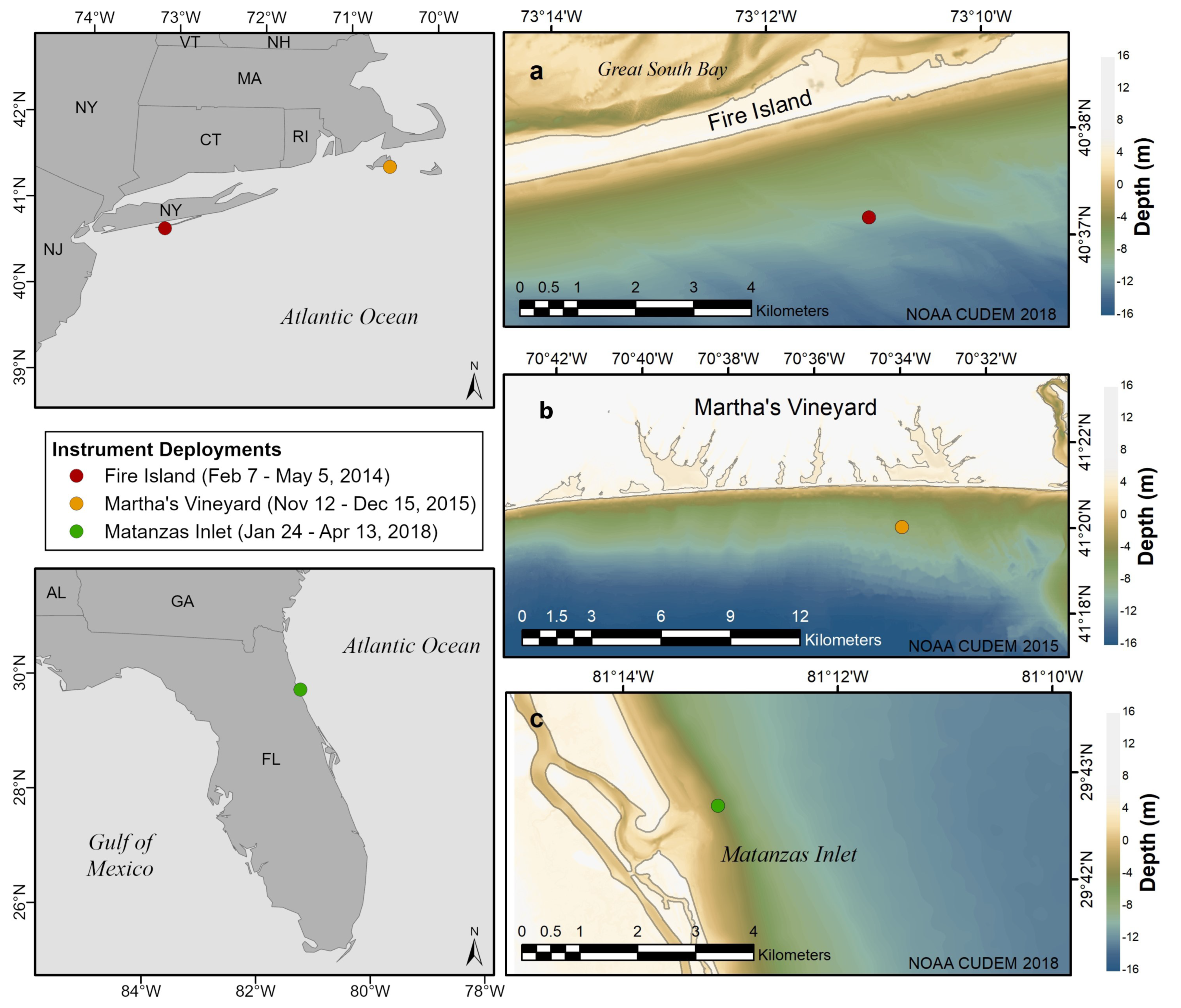
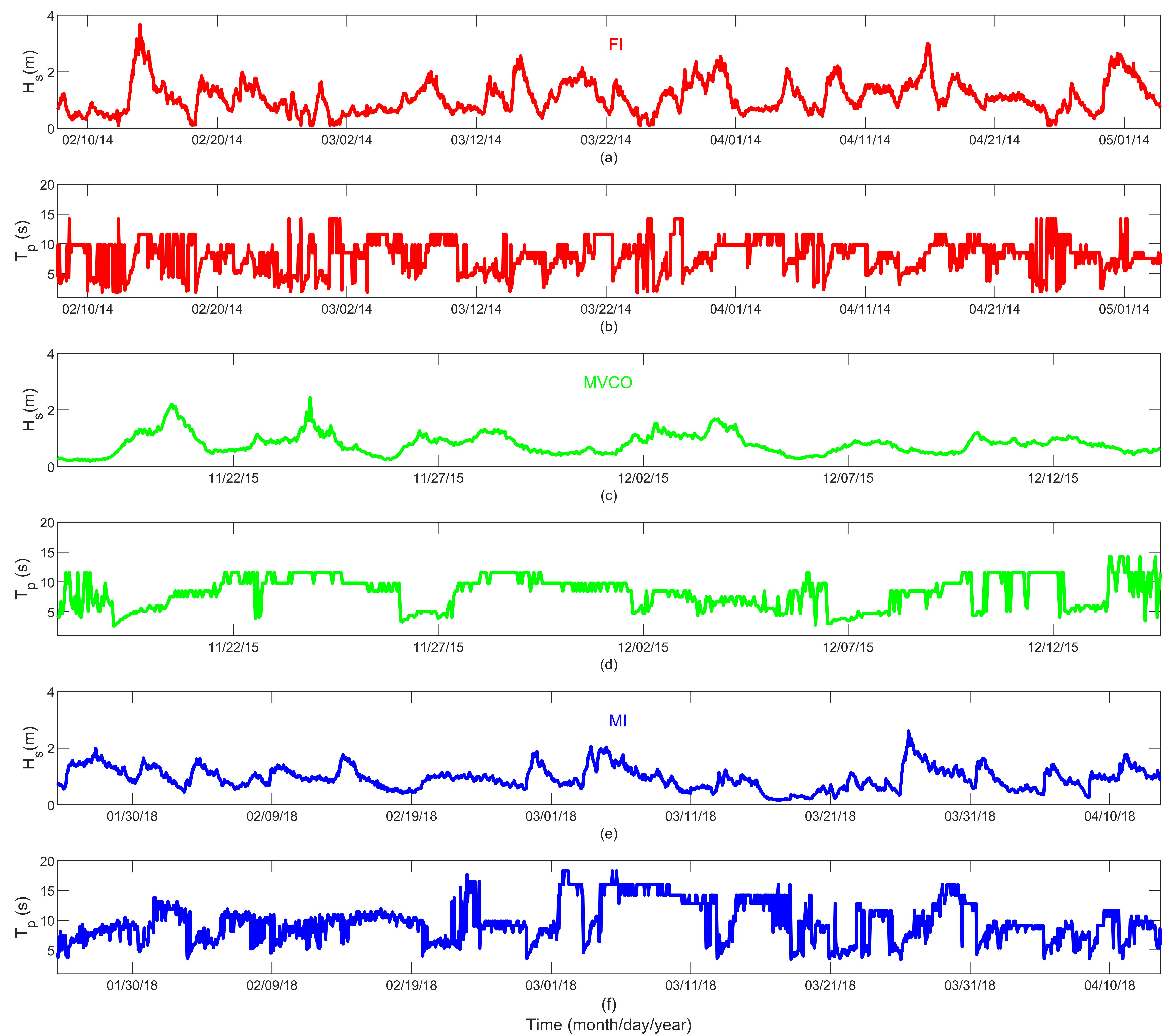
2.1. Field Study Sites

The datasets used in the present work were obtained at three field study sites: Fire Island, New York (FI), Martha’s Vineyard Coastal Observatory, MA (MVCO), and Matanzas Inlet, FL (MI). The FI dataset was part of a field campaign [40,41] to study the along-shore variations in waves and sediment processes. FI data from the site shown in Figure 1a correspond to a mean depth of 16 m located approximately 2 km offshore from the southern shoreline of western Fire Island in New York. The MVCO dataset [42] was collected at a site with an average depth of 14 m offshore located approximately 2 km from the southern shoreline of Martha’s Vineyard (Figure 1b). The Matanzas Inlet dataset was collected [43] to study the effects of cross-shore currents on waves, and measurements were made at a site with an average depth of 9 m located approximately 0.8 km offshore from the eastern shoreline (Figure 1c).

Table 1. Filenames containing the datasets used to obtain near bottom and surface wave measurements.

Wave Parameter	Fire Island, NY (40.6193, −73.1840)	MVCO, MA (41.3337, −70.5659)	Matanzas Inlet, FL (29.7114, −81.2186)
ADV burst	9917advb-cal.nc	10577vecb-cal.nc	11109vecb-a.nc
ADV burst statistics	9917advs-cal.nc	10577vecs-a.nc	11109vecs-a.nc
Workhorse	9921whp-cal.nc	10571whVp-cal.nc	11101whVp-cal.nc and
Seabird Seaguage	-	-	-
Sonar	-	-	11107hffan_raw.cdf
ADV burst	9917advb-cal.nc	10577vecb-cal.nc	11109vecb-a.nc

mentions the filenames containing the datasets used to obtain near bottom and surface wave measurements.

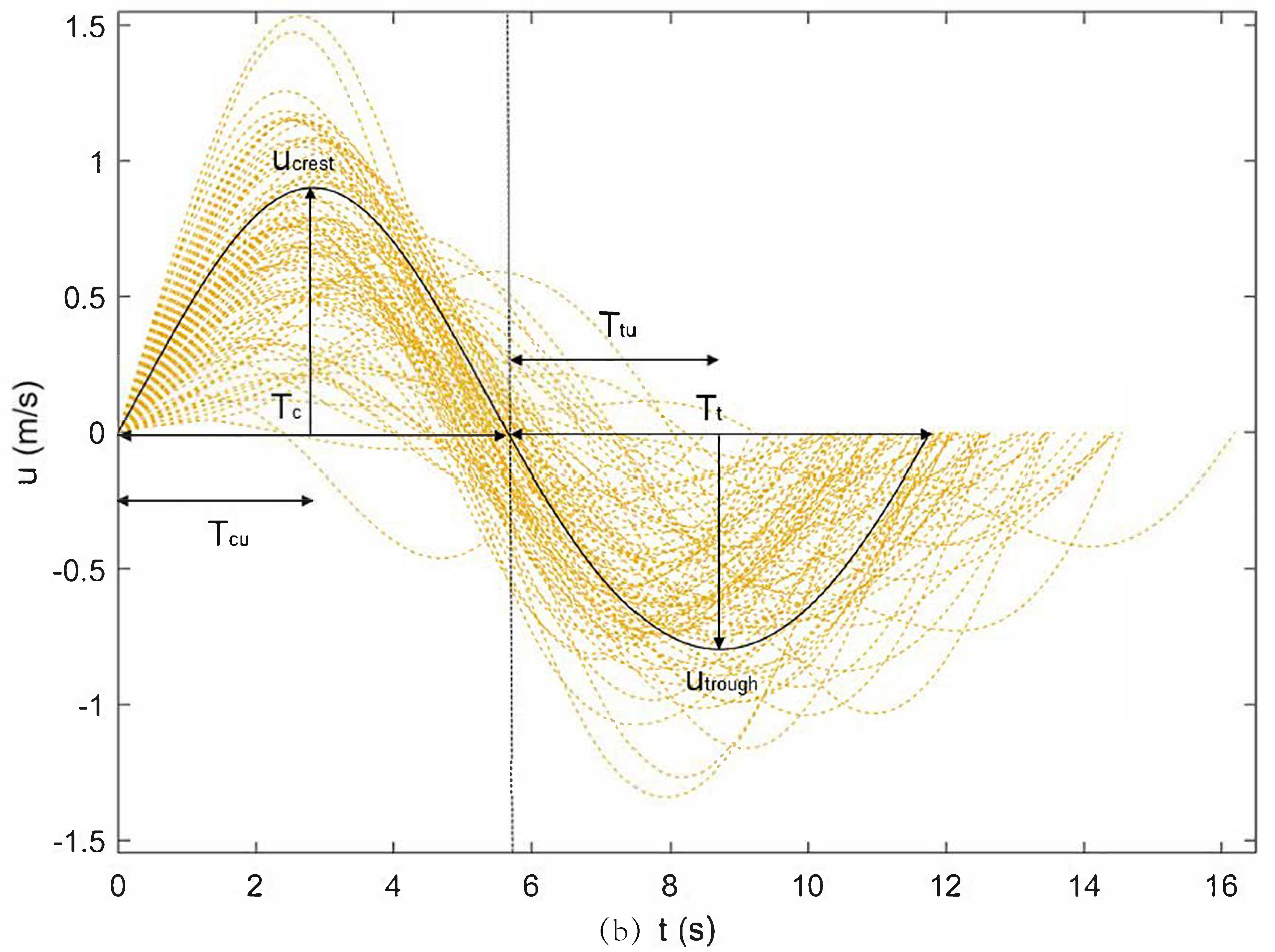
2.2. Parameterized Method: Skewed Waveform Estimation from Surface Wave Data

The parameterized method to compute the near-bottom wave forms uses surface bulk wave parameters. The parameterized method to find skewed waveform characteristics ($u_{crest}$, $u_{trough}$, $T_c$, $T_t$, $T_{cu}$, $T_{tu})$ is described in Appendix A and requires local values of significant wave height $H_S$, a representative wave period $T$, depth $h$, and wave orbital velocity amplitude $u_w$. Surface wave spectra were measured with an acoustic Doppler current profiler (ADCP; Table 1). The ADCP beam orbital velocities measured at bins near the surface were used to calculate wave spectra at the three sites using the WavesMon software. An exception to this methodology was the Matanzas Inlet site where, after the first 31 days of the 80-day deployment, measurements from a near-bed pressure sensor (SeaBird Seagauge) were substituted because the ADCP malfunctioned. In these pressure-sensor data, the mean $H_S$ was 7% smaller and the mean $T_p$ was 8% larger than those measured with the ADCP for the 31 days when both the sensors worked. The methods described by [44] were used to obtain near-bed estimates of $u_w$ and $T$ from the surface wave spectra. Note that for the application of Appendix A, we used a representative wave period ($T$) that was defined as $T$ = $\frac{m_0}{m_1}$, where $m_0$ is the variance of water surface elevation and $m_1$ is the first moment of the spectral density of surface elevation.

Table 2. ADCP sensor specifications for the three sites. The sensor height for the velocity measurements changed during the deployment period but the median elevation remained around the nominal elevation (latitude and longitude in decimal degrees).

Site Location	Fire Island, NY (40.6193, −73.1840)	MVCO, MA (41.3337, −70.5659)	Matanzas Inlet, FL (29.7114, −81.2186)
Collection period	7 February–5 May 2014	12 November 15–December 2015	24 January–13 April 2018
Sensor type	RD Instruments ADCP	TRDI V	TRDI V
Instrument frequency	600 kHz	1000 kHz	1000 kHz
Burst sampling rate	2 Hz	2 Hz	2 Hz
Burst sampling length	1024 s every hour	1024 s every hour	2048 s every hour
Initial instrument elevation above bottom	2.1 m	2.4 m	2.4 m

provides sensor specifications used from each of the three sites. The characteristics of the parameterized waveform obtained using this method are described later with the use of subscript “($p$)”.

2.3. Direct Method: Skewed Waveform Estimation from Near-Bed Data

The direct method uses near-bed observations to determine a representative skewed waveform. Waveforms were observed directly from near-bed velocity measurements made with acoustic Doppler velocimeters (ADVs;

Table 3. ADV sensor specifications for the three sites. The sensor height for the velocity measurements changed during the deployment period (distance to the measurement volume).

Site Location	Fire Island, NY	MVCO, MA	Matanzas Inlet, FL
Collection period	7 February–3 May 2014	17 November–8 December 2015	24 January–13 April 2018
Sensor type	Sontek ADV	Nortek Vector ADV	Nortek Vector ADV
Instrument acoustic frequency Burst sampling rate	5000 kHz 8 Hz	6000 kHz 16 Hz	6000 kHz 16 Hz
Burst sampling length	1050 s every hour	1875 s every hour	2048 s every hour
Measurement location (height above bed)	0–35 cm	64 cm	20–40 cm
Pressure sensor height	1.14–1.5 m	1.69 m	1.97 m

). The measured time series of wave velocity directly obtained from ADV recordings are in two components, $u_{raw}$ and $v_{raw}$ close to the seafloor in bursts (ref. Table 3 for site-specific burst length) at an elevation close to the seafloor but above the wave boundary layer. The process is described here for one component, that is, $u_{raw}$ for the sake of brevity; a similar analysis was performed for $v_{raw}. u_{raw}$ was decomposed into a slowly varying mean tidal component $\langle u\rangle$, an incident-wave band ${\tilde{u}}_{incident}$, an infragravity wave band ${\tilde{u}}_{infragravity}$ and noise associated with turbulence and instrument error $u^{\prime }$.

$$u_{raw}=\langle u\rangle +{\tilde{u}}_{incident}+{\tilde{u}}_{infragravity}+u^{\prime }$$

(1)

Velocities from each burst time series were first detrended to remove $\langle u\rangle$. Incident-wave velocities ${\tilde{u}}_{incident}$ with periods of 4–20 s were isolated using a Butterworth bandpass filter. The lower limit of 4 s removed higher-frequency motions that were assumed to not affect the calculations of bedload at the bottom, thus reducing the noise in the signal. The upper limit of 20 s excluded waves in the infragravity band. The infragravity band was removed so that only the sea-swell frequency band remained, to match the frequency range in Ruessink’s data [34] and to apply an asymmetric bedload-transport equation that was formulated with the exclusion of the infragravity band. Figure 2 compares the raw and incident wave spectrum from a storm event in the Fire Island dataset that corresponds with an $H_S$ of 3.7 m associated with a corresponding $T_P$ of 11.6 s.

A principal components analysis (PCA) was applied to the ${\tilde{u}}_{incident}$ and ${\tilde{v}}_{incident}$ wave signals to determine the axis of dominant wave motions. PCA determined the dominant wave direction and the corresponding velocity signal (referred to as $\tilde{u}$) for each burst. Representative waveforms were found within burst time series by (a) identifying individual waves using zero-up crossings, (b) determining characteristics ($u_{crest}, u_{trough}$, $T_{crest}$, $T_{trough}$, $T_{cu}$, and $T_{tu}$) of the individual waveforms, (c) calculating parameters that describe waveform according to the formula of [3], and computing a weighted average of those parameters. Zero up-crossings times were used to find short time series of velocity $u\left(t\right)$ with period $T_i$ for each wave in the time series, where subscript “$i$” refers to the individual waveforms in a wave burst time series. From these individual wave motions, the crest and trough velocities $u_{c,i}, u_{t,i}$ and crest and trough periods $T_{c,i}$ and $T_{t,i}$ were determined. In the next step, three parameters corresponding to the individual waveforms were calculated that included the amplitude of wave orbital velocity as defined by:

$$u_{w,i}=0.5 \left(u_{c, i}-u_{t, i}\right)$$

(2)

and their velocity skewness ($R_i$) according to [45]:

$$R_i=\frac{u_{c, i} }{\left(u_{c, i}-u_{t, i}\right) }$$

(3)

The inputs of non-dimensional $u_{w,i}$, $T_i$ and $R_i$ were used to calculate the third parameter $b_{1,i}$ a fitting parameter that results in a free-stream velocity description [3] by finding the maximum and minimum positions of velocity in the individual waveforms. The equations to calculate $b_{1,i}$ are provided in the Matlab script “abreu_fit” provided by [46]. The weighted means of individual waveform $u_{w,i}$, $T_i$, $R_i$, and $b_{1,i}$ were used in the Matlab script “abreu_fstream” [46] to obtain the representative waveform for each burst time series (Figure 2b as an example). Weighting was based on the product of the squared wave-orbital amplitude and wave period, as:

$$w_i=u_{w,i}^2{T}_i$$

(4)

The characteristics of the parameterized waveform obtained using this method are described later with the use of subscript “$d$”.

2.4. Calculation of Bedload for Skewed Waveforms

We derived three estimates of wave-driven cross-shore bedload transport using the Matanzas Inlet dataset because that site had the highest proportion of skewed waveforms (Section 3.4). Both the parameterized and direct skewed waveforms were used to drive a bedload transport formulation that accounted for skewed waves [38], referred to as asymmetric bedload formulation. Results were also calculated using a traditional excess-stress bedload formulation, the Meyer–Peter and Müller (MPM) equation [39]. Appendix B and Appendix C detail the equations used for the asymmetric and MPM formulations. The grain size used in the calculations was $d_{50}=0.23 \mathrm{mm}$ [43]. In contrast to the asymmetric bedload formulations, which represent waveforms with wave asymmetry indices, the MPM formulation (Equation (A43)) uses the entire time series of instantaneous wave motions (${\tilde{u}}_{incident})$ in the bedload calculations.

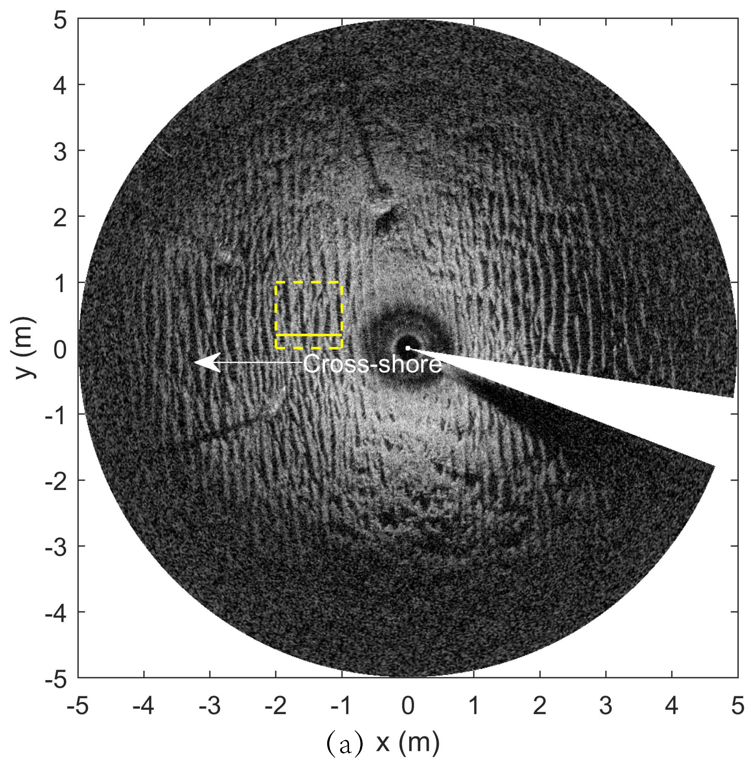
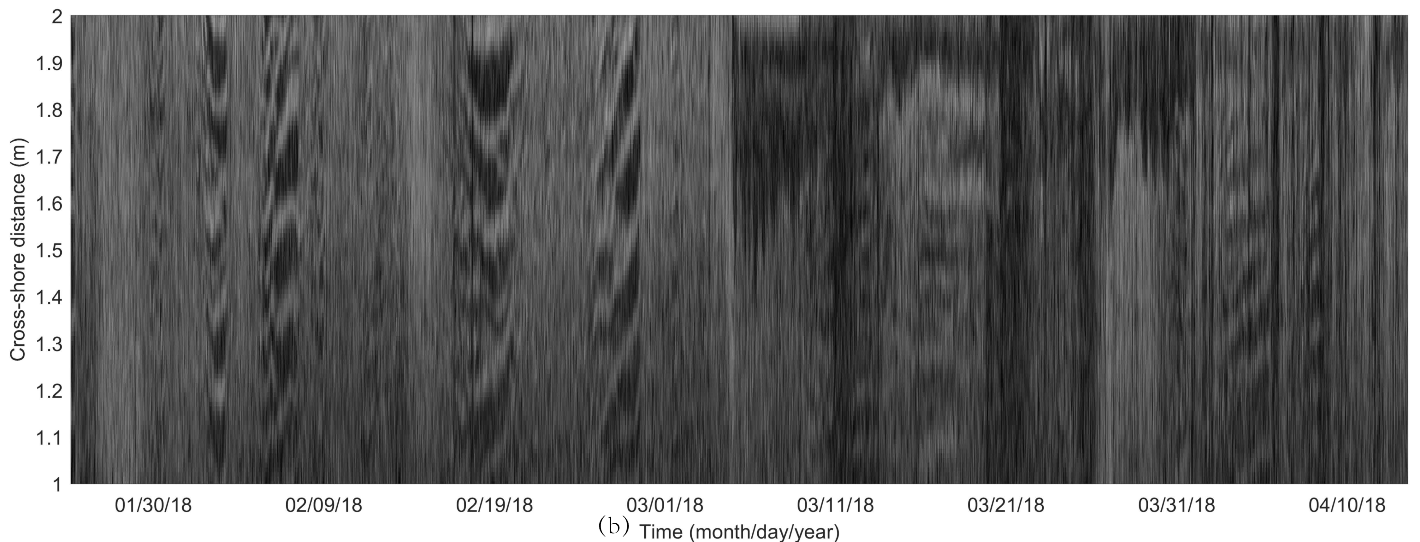
2.5. Sonar Imagery for Bedform Transport Rate from Ripple Migration

Measurements of bedform transport, a proxy for bedload transport, were determined from sonar imagery that tracked ripple migration on the seafloor. The analysis was performed for the shallowest site (Matanzas Inlet) where good images of active ripple migration were available. Images of the seabed were obtained every 30 min from a 2.25 MHz Imagenex model 881A fan-beam rotating imaging sonar mounted 0.45 m (nominal) above the bed. The raw images of backscatter intensity from the sonar were corrected for slant range and rotated into geographical coordinates (positive x = east). This resulted in images with a horizontal resolution of 0.01 m and covering a circular region with a 5 m radius (Figure 3a). In these images, the light and dark pixel values corresponded to acoustic backscatter intensity (light indicates high backscatter that revealed the presence of ripples). Manual inspection was used to find a region with ripples that were well defined for most of the time series. This corresponded to a 1-m × 1-m square (Figure 3a) orientated in the onshore direction located 1–2 m from the center of the image. The ripple wavelength $\left({\lambda }_r\right)$ was determined in the sub-patch region using the two-dimensional fast Fourier transform method described in these studies [47,48,49,50].

We used a single cross-shore transect (shown in Figure 3a) located at 0.05 m distance from the southern edge of the square to form a time-stacked image (Figure 3b). Manual trials showed that the quality of the time stacked image remained unchanged for ripple tracking purposes by choosing any other current transect within the square region. The cross-shore position of pixel intensity was determined using edge detection [51,52]. The cross-shore migration rate ($d_r$) was determined as the change in cross-shore position at half-hour intervals. The resulting volumetric bedform transport rates ($\overrightarrow{q_b},$ ${\mathrm{m}}^3/\mathrm{m}$) estimated from the sonar data were computed [11] as:

$$\overrightarrow{q_b}=\left(1-\epsilon \right)f_r{\eta }_r{d}_r$$

(5)

assuming a bed porosity factor $\epsilon =0.4$, dimensionless ripple shape factor $f_r=0.5$, and a constant ripple height to ripple wavelength ratio $\frac{{\eta }_r}{{\lambda }_r}=0.16$ [11].

3. Results

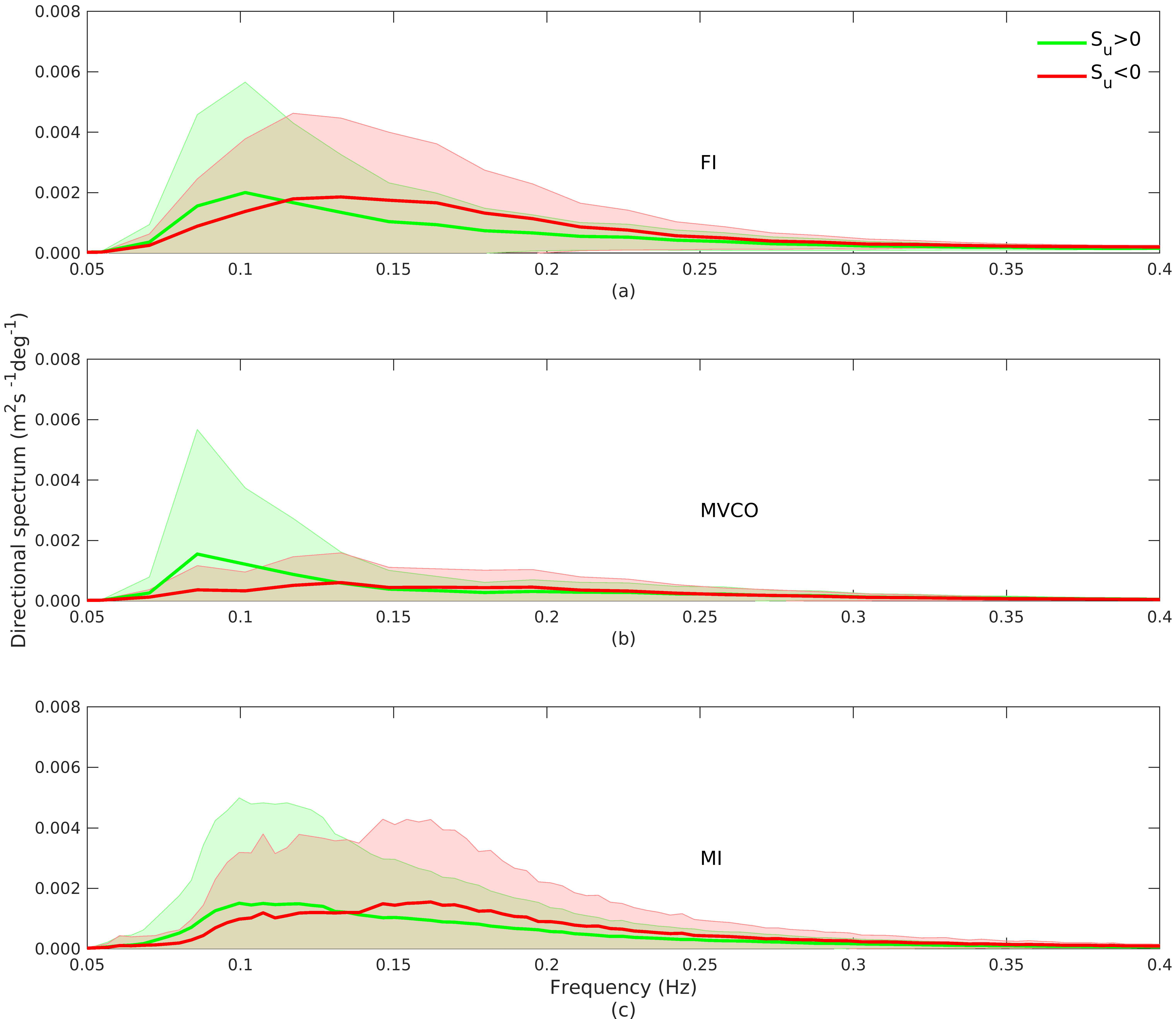
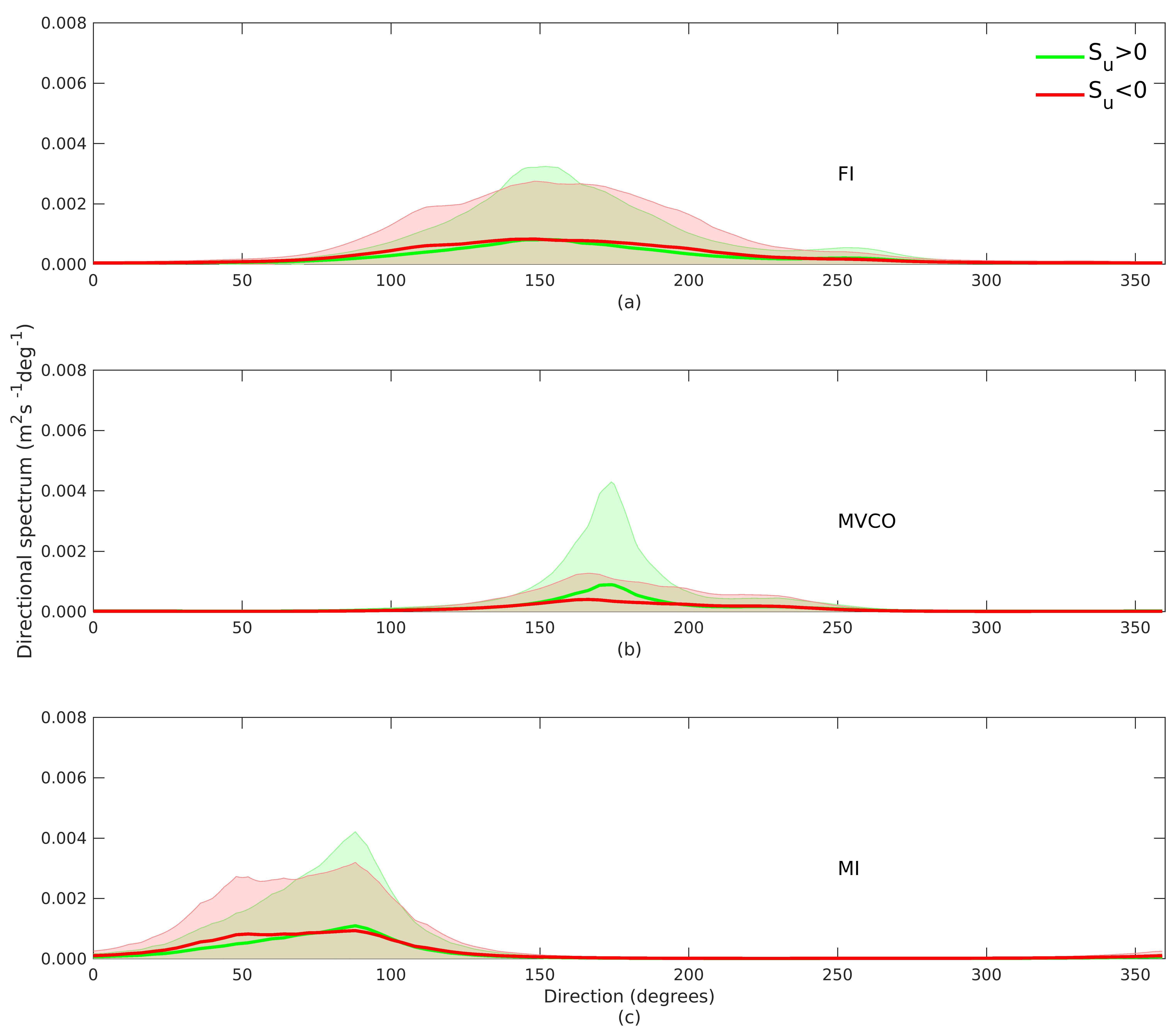
3.1. Surface Wave Statistics

MVCO had the least-energetic waves of the three sites (Figure 4). Fire Island was the deepest site and had the highest proportion of high $H_S$. Matanzas Inlet had the highest proportion of waves with high $T_P$. Energetic waves (high $H_S$ and $T_P$) and shallower water depths would be expected to generate larger wave skewness.

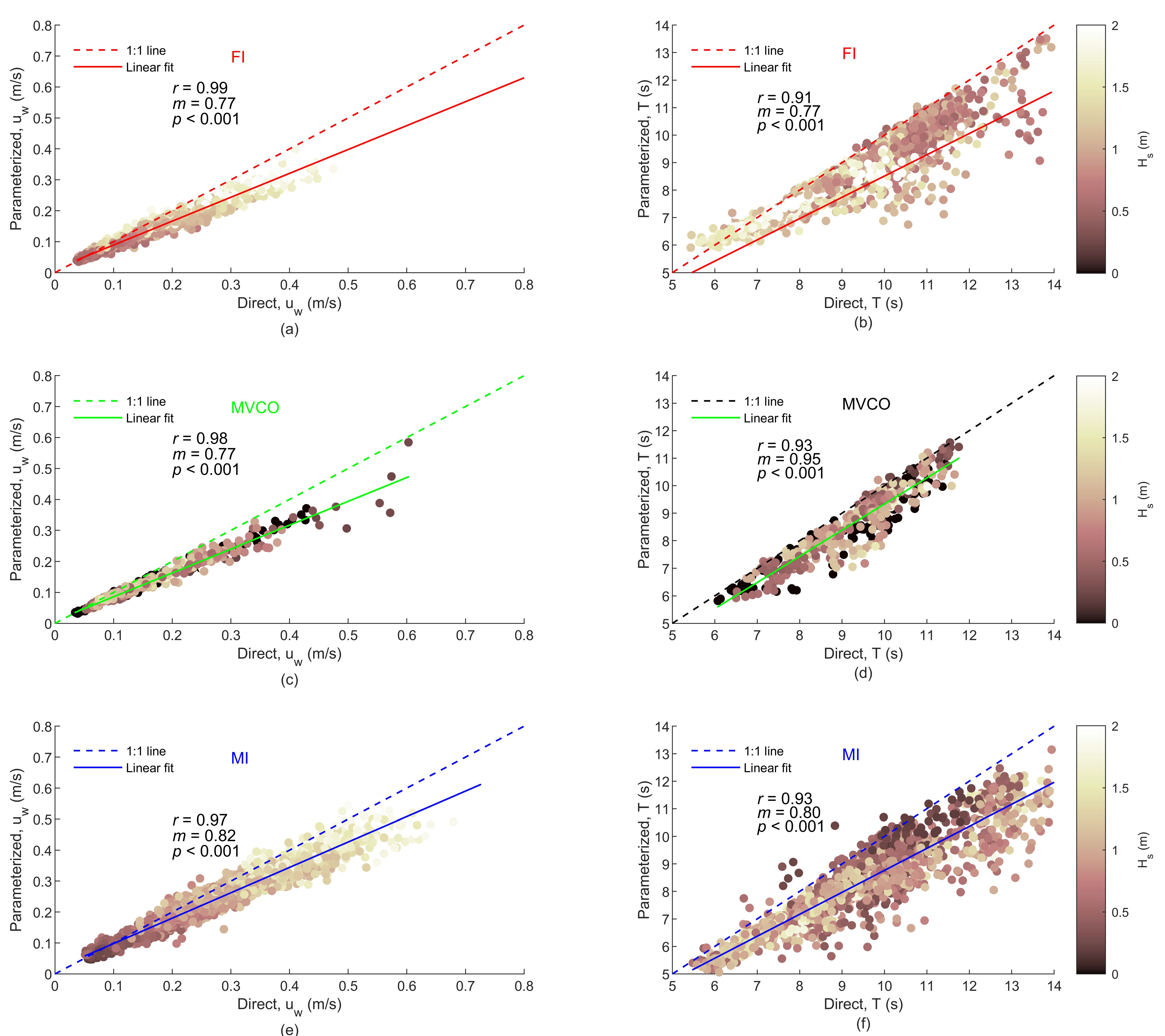
3.2. Comparison of Representative Wave Period and Orbital Velocity from Surface Wave Data and Near-Bed Wave Data

Peak wave orbital velocity (u_w,d and u_w,p) and representative wave periods (T_w,d and T_w,p) are compared in Figure 5 for the three sites, based on both (parameterized and direct) methods described in Section 2.2 and Section 2.3 where subscript “w” refers to the representative waveforms obtained from the two methods (parameterized and direct). The correlation (Pearson’s correlation coefficient, r) between u_w,d and u_w,p was above 90% at all three sites and the best linear fit (identified by the slope value) was obtained at the shallowest site (Matanzas Inlet; Figure 5a,c,e). At Fire Island and Matanzas Inlet, u_w,p was underpredicted compared to u_w,d as significant wave heights (H_s) increased (Figure 5a,e). The correlation between T_w,d and T_w,p was found to be above 90% at all three sites (Figure 5b,d,f). T_w,p was consistently underpredicted compared to T_w,d at all three sites for almost all wave heights. This pattern can be attributed to the damping of high-frequency motions in the near-bottom measurements, leading to relatively higher values of T_w,d. The linear fits to T_w,d and T_w,p were better in the shallower depths at MVCO (Figure 5d) and Matanzas Inlet (Figure 5f), compared to those at Fire Island (Figure 5b).

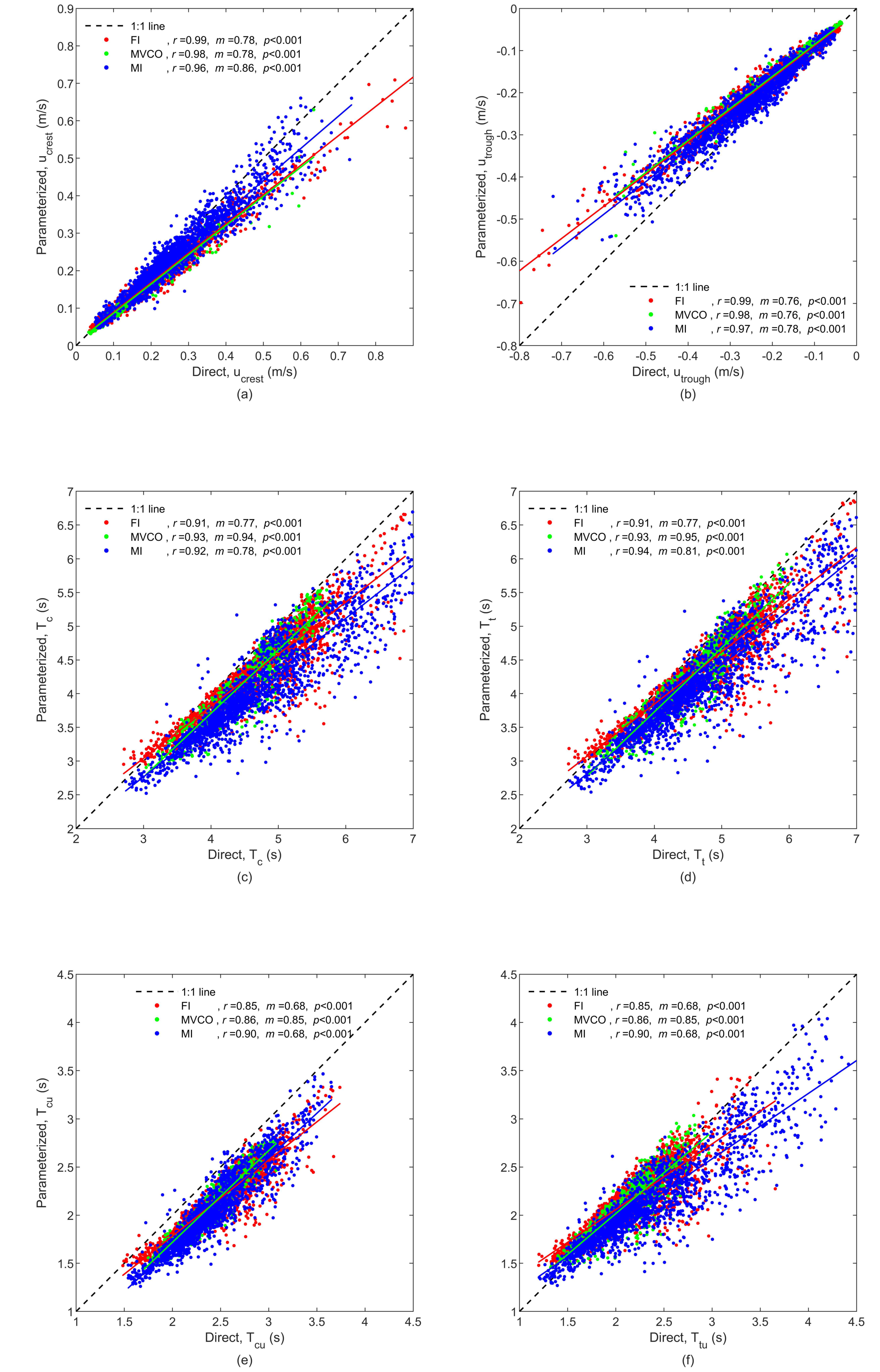
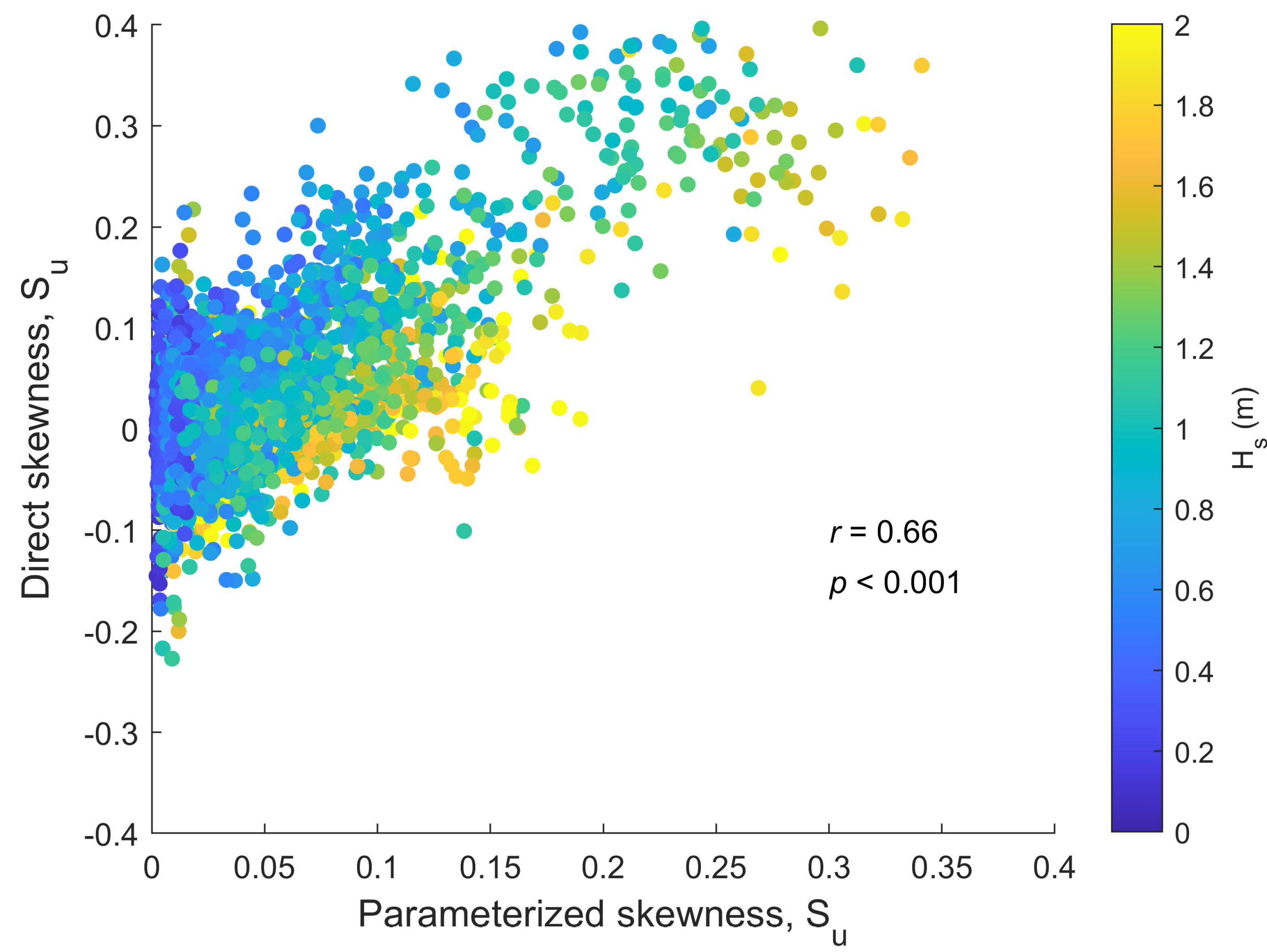
3.3. Skewed Waveform Characteristics: Parameterized and Direct Methods

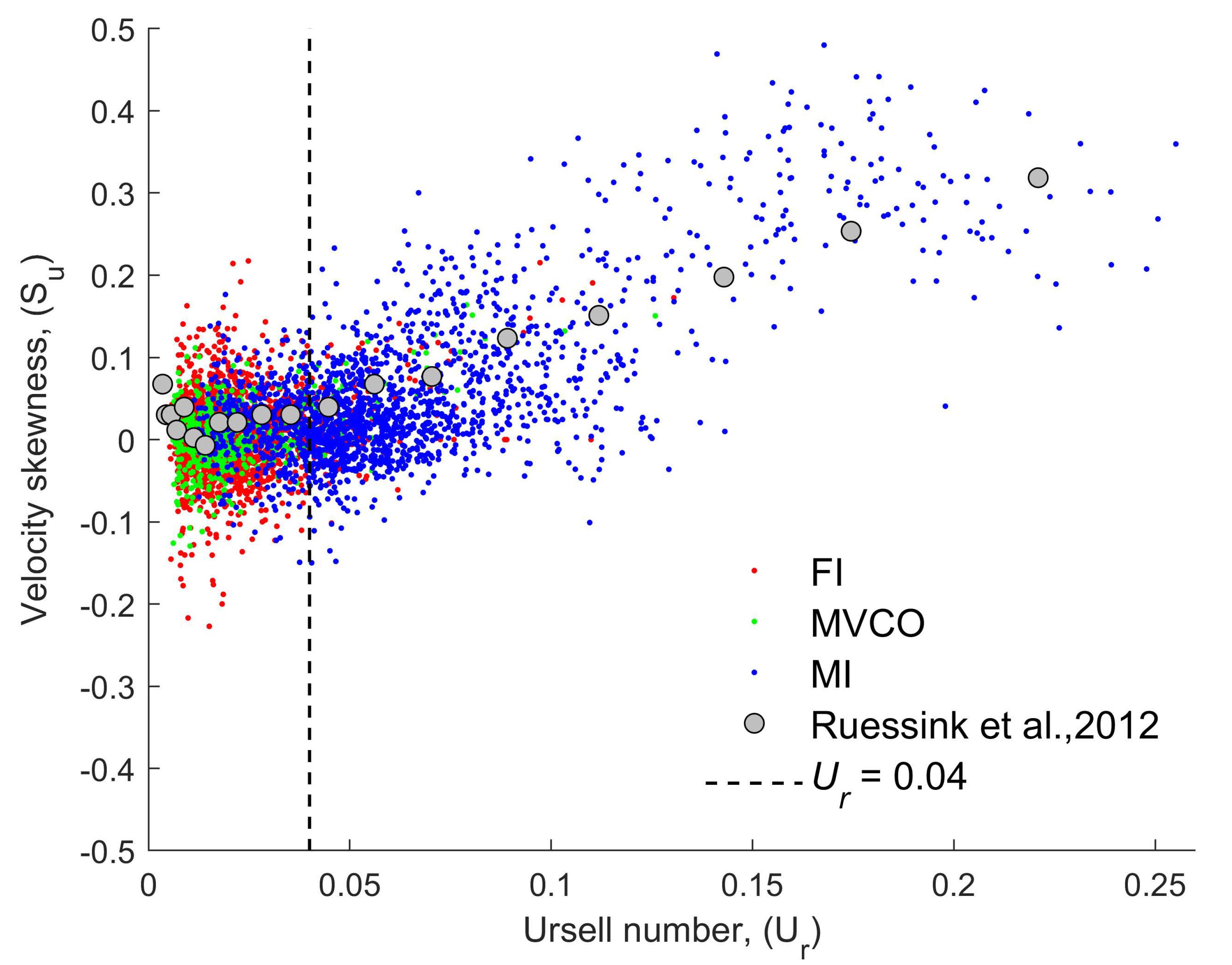
We used the equations described in Appendix A and methods described in Section 2.2 and Section 2.3 to determine the parameterized and direct representative skewed waveform characteristics which included $u_{crest}$, $u_{trough},$ $T_c$, $T_t$, $T_{cu}$, and $T_{tu}$. These characteristics were used to calculate the wave-driven bedload calculations (Appendix B). The comparison of $u_{crest,d} \mathrm{and} u_{crest,p }$ (Figure 6a) and $u_{trough,d} \mathrm{and} u_{trough,p}$ (Figure 6b) showed a $r>0.9$ and that linear fit improved for the Matanzas Inlet site compared to the other two sites. The correlations between $T_{c,d} \mathrm{and} T_{c,p }, T_{t,d} \mathrm{and} T_{t,p }, T_{cu,d} \mathrm{and} T_{cd,p } \mathrm{and} T_{tu,d} \mathrm{and} T_{tu,p }$ remain high ($r>0.85$) (Figure 6c–f). The pattern of linear fit for half periods was consistent with the results of the representative wave period (i.e., Figure 5b,d,f).

The E₁ error was highest for the shallowest site of Matanzas Inlet for all waveform characteristics (

Table 4. Errors between direct and parameterized waveform characteristics at all three sites where E₁ = $RMS{E}_i$ and E₂ = $100\left(RMS{E}_i\right)/RM{S}_{id}$ where subscript “i” is for an individual waveform characteristic and subscript “d” refers to the direct method.

Wave Parameter	Fire Island, NY		MVCO, MA		Matanzas Inlet, FL
	E1	E2	E1	E2	E1	E2
uw (m/s)	0.04	19.63	0.04	20.62	0.05	15.89
T (s)	0.91	9.50	0.78	8.44	1.34	13.88
ucrest (m/s)	0.04	19.02	0.04	20.17	0.04	14.76
utrough (m/s)	0.04	20.28	0.04	21.13	0.05	17.48
Tc (s)	0.46	9.64	0.40	8.71	0.69	14.61
Tt (s)	0.44	9.25	0.38	8.23	0.65	13.28
Tcu (s)	0.35	13.89	0.32	12.30	0.38	15.94
Ttu (s)	0.21	9.09	0.17	7.96	0.34	14.17

). E₂ error that accounted for scaling the error with the RMS values showed that the Matanzas Inlet site had the least error corresponding to the velocity characteristics of the waveform ($u_w, u_{crest}$, $u_{trough}$). On the contrary, E₂ error was highest for period characteristics ($T, T_c$, $T_t$, $T_{cu}$, and $T_{tu}$) at the Matanzas Inlet site.

3.4. Wave Skewness

Wave-orbital velocity skewness drives bedload transport and can be used as a diagnostic tool to indicate transport potential. Non-dimensional wave-orbital velocity skewness (hereafter referred to as skewness, $S_u$) was calculated at the bottom using the ADV-based direct method as:

$$S_u=\frac{\langle {\tilde{u}}^3\left(t\right)\rangle }{{\left({\tilde{u}}_{rms}\right)}^3}$$

(6)

where $\tilde{u}$ is wave-orbital velocity, angle brackets indicate time-averaging over the burst, and subscript rms indicates root mean square over the burst. $S_u$ tends to increase with Ursell number ($U_r$) above a threshold of about $U_r=0.04$ (Figure 7). This is consistent with the observations of [34] who mentioned that $U_r\le 0.04$ have near-zero skewness. Most of the observations at the two deeper sites (93% at FI and 75% at MVCO) fell below this threshold. In contrast, only 25% of the MI data had a $U_r\le 0.04$.

For $U_r>0.04$, about 22% of the waveforms at MI were associated with negative skewness (similar to the results in [34]) (Figure 7). We examined the directional wave spectrum, $D_{spec}=f\left(\omega ,\theta \right)$ of bottom skewness, where $\omega$ is the frequency in Hz and $\theta$ is the direction in degrees to determine whether negative skewness was related to spectral characteristics. The events associated with positive and negatively skewed waves ($S_u$) in the directional wave spectrum were binned separately. We first averaged $D_{spec}$ along all directions to get mean frequency spectra ($\langle D_{spec-\omega }\rangle$, Figure 8). The spectra associated with positive $S_u$ (green shaded region) frequencies are shifted toward lower frequencies compared to spectra associated with negative $S_u$ (red shaded region), which are shifted towards higher frequencies at all three sites (Figure 8a–c). Positively skewed waves also had narrower frequency distributions. The differences in mean frequency and standard deviation about the mean for spectra with positive versus negative skewness were significant with ($p<0.01$). We also found that the statistical skewness of the spectral distributions was higher for positively skewed waves (significantly different with $p<0.001$). This pattern confirmed a shift of the spectral distribution towards lower frequencies associated with positively skewed waves.

Next, we averaged $D_{spec}$ across all frequencies to get spectra $(\langle D_{spec-\theta }\rangle )$ varying over direction and binned based on the sign of skewness (Figure 9a–c). Positively skewed waves (green lines) were associated with a smaller directional spread of energy while negatively skewed waves (red) corresponded to a larger directional spread of energy (Figure 9a–c). This was confirmed by the kurtosis of the direction distributions, which was significantly different ($p<0.001$) with positively skewed waves exhibiting more peakiness (leptokurtic), and negatively skewed waves exhibiting broader directional spread, especially at MVCO. In summary, data from all three sites (Figure 8 and Figure 9) show that spectra associated with positively skewed waves were distributed over a lower peak frequency with a narrower directional spread. Conversely, spectra for negatively skewed waves were distributed over higher frequencies and with a larger directional spread of energy at all three sites. A similar pattern was noticed in data [12] from an 18-h storm event. They concluded that the sign of the skewed waves originated from wave-wave interactions, and the spectral shift towards higher frequencies originated from mixed sea and swell conditions, whereas unimodal swell conditions with lower frequencies led to positive skewness, consistent with Figure 8.

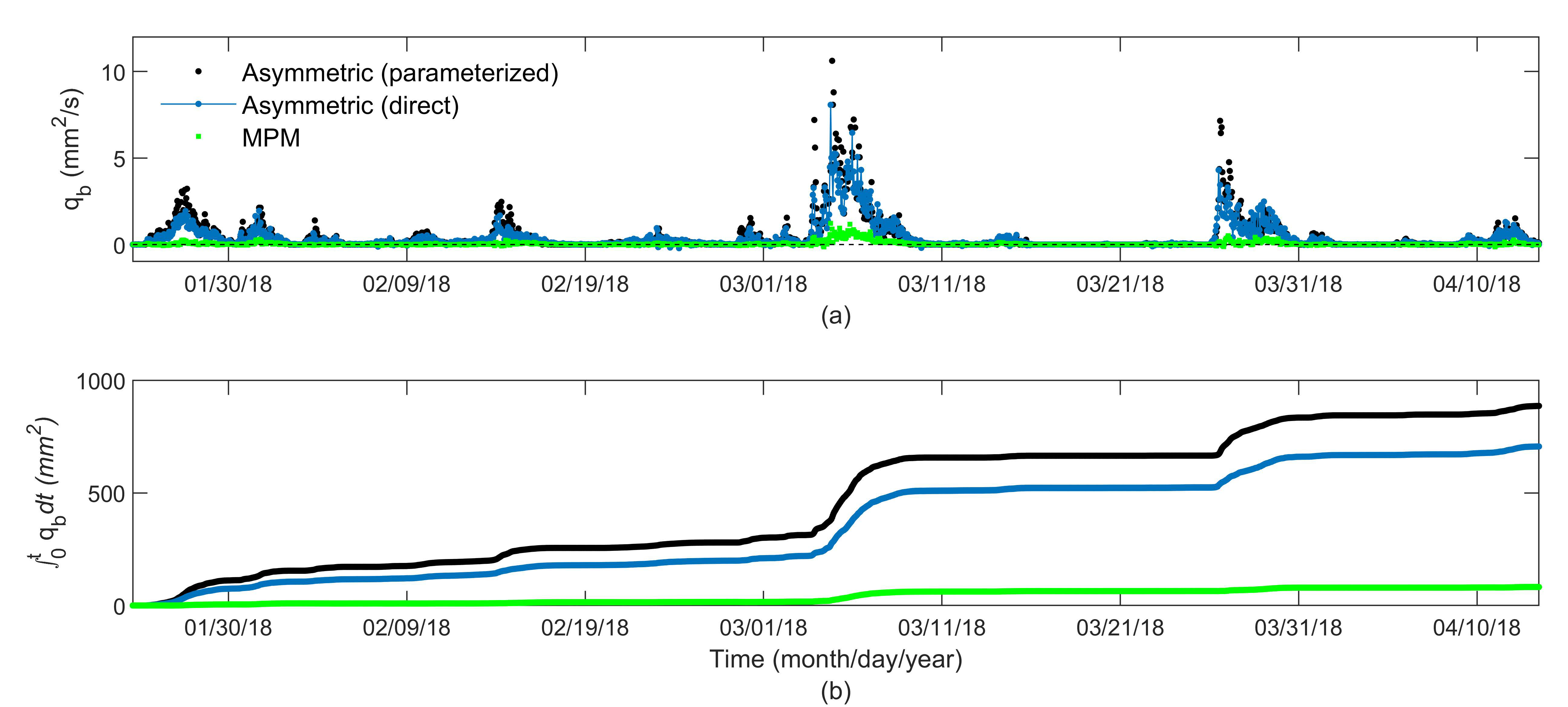
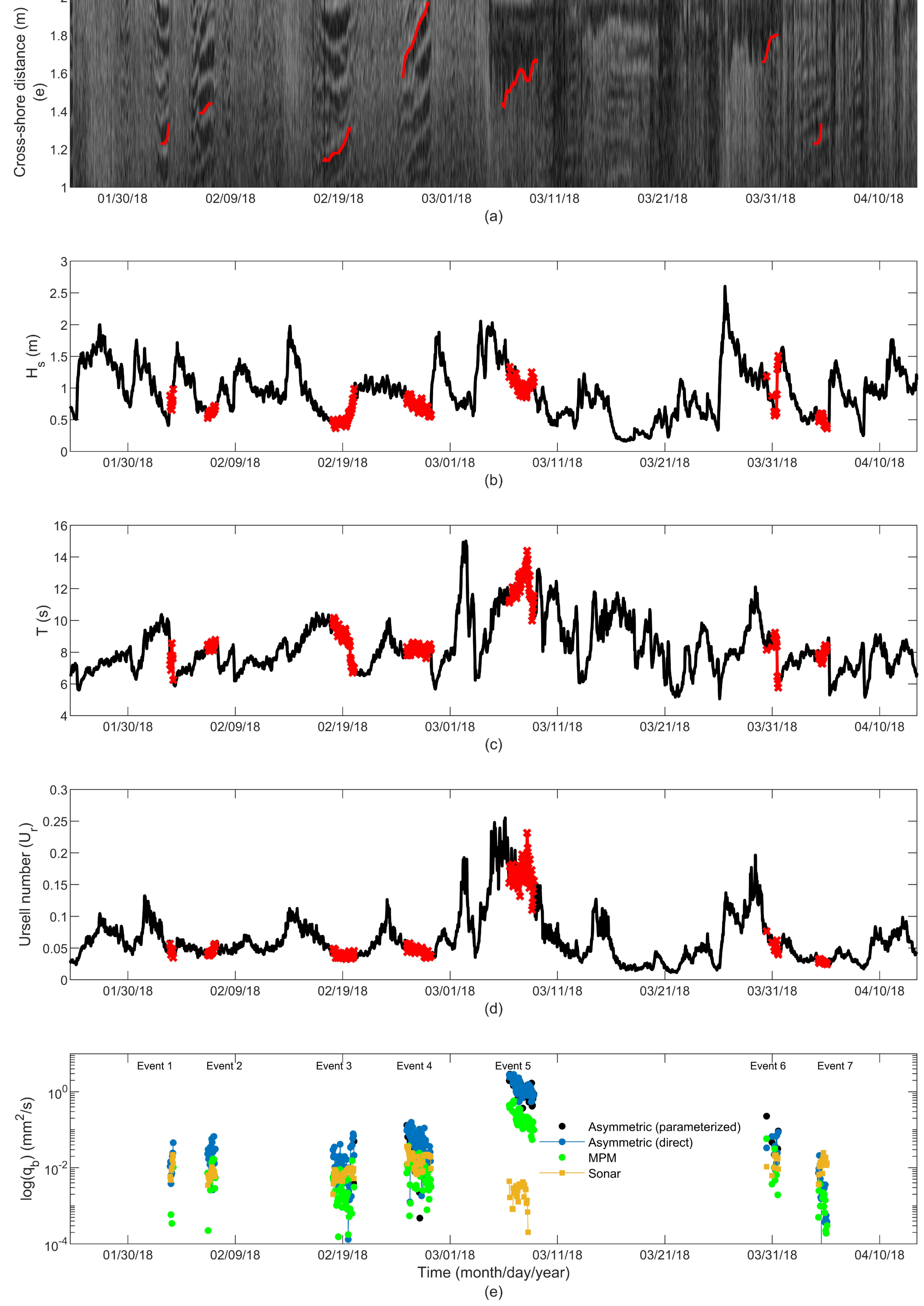
3.5. Estimating Wave-Driven Cross-Shore Bedload Using Skewed Waveform Parameters

We compared our three estimates of wave-driven cross-shore bedload transport (Section 2.4) using the Matanzas Inlet dataset because that site had the highest proportion of skewed waveforms (Section 3.4). The first two estimates were calculated using a slightly modified version of the SANTOSS formula ([38]; Appendix B). This formula requires estimates of wave asymmetry and calculates transport separately for each part of the wave cycle. We derived asymmetry values from surface waves (our “parameterized” method using the [34] approach; Appendix A) and from near-bottom measurements (our “direct” method; Appendix B) and compared it with a traditional excess stress-based bedload formulation (i.e., the MPM method detailed in Appendix C). Figure 10a,b compare instantaneous ($q_b$) and time-integrated net (${\int }_0^t{q}_{b }dt$) bedload transport rates where positive values in Figure 10a indicated bedload along the wave aligned axis and negative values are opposite to that. The bedload values reach local peaks during similar time intervals between all three methods and are associated with high wave energy events (refer to Figure 4) that result in larger skewness (Figure 10a). The parameterized method’s $q_b$ exceeded the direct one during 51% of time instances because it always predicted a positive skewness and as a result, the parameterized $q_b$ showed an increase of 25% in the (${\int }_0^t{q}_{b }dt$) (Figure 10b). In both the direct and MPM method, there is a change in the sign of $q_b$ during certain periods although the magnitude of negative $q_b$ is much smaller over the entire time series for both methods. For all the events where $q_b>0$, the (${\int }_0^t{q}_{b }dt)$ with MPM method was 700% smaller when compared to the direct skewed waveform based (${\int }_0^t{q}_{b }dt)$.

Analysis of the time-stacked ripple images identified seven periods that were continuous, which allowed tracking of the ripple front. Manual interpretation (red lines, Figure 11a) was used to detect the starting and ending point of each continuous period. The ripple wavelength in these periods ranged from 0.065 to 45 cm. Using the distance traversed by ripple wave fronts over the duration of each segment, we found ripple migration rates ranging from 0.3 cm/day to 0.48 cm/day. The corresponding significant wave height ($H_s$) and representative wave period ($T$) at the bottom ranged between 0.4 to 1.5 m and 5.8 to 14.4 s respectively (Figure 11b,c). The Ursell $(U_r)$ number during these periods ranged from 0.024 to 0.23 (Figure 11d). The relatively low values of these parameters (Figure 11b–d) for the periods when ripples could be tracked suggest the sonar was only capable of providing bedform transport estimates during weak events. During other times, ripples were not clearly visible in the images.

A comparison of instantaneous $q_b$ from sonar imagery and empirical methods (Figure 11e; note logarithmic y-axis) shows that there was substantial scatter within events, and that the four methods often overlapped. The $q_{b }$ estimates are typically within 2 orders of magnitude with each other. The exception is the strongest event, between 06–09 March, when the sonar $q_{b }$ estimates were lower than $q_{b }$ calculated from both the asymmetric waveform methods and the MPM method. There are periods (02–03 February, 06–07 February, and 03–04 April) when the parameterized method results in zero $q_b$ (not visible on the logarithmic axis) because the calculated stress did not exceed the threshold critical stress in crest or trough cycles.

The RMSE of the cumulative bedload calculated from the asymmetric bedload method is lower than MPM for two events (1 and 7) but in all other events, it is greater (

Table 5. Event-based cumulative error (RMSE) and correlation coefficient (${\mathrm{r}}_1$) between the calculated transports (both asymmetric direct and MPM) and the sonar estimates. Significant correlations (p < 0.05) are indicated in bold.

Event Period	Asymmetric (Direct)		MPM
	RMSE	${\mathbf{r}}_1$	RMSE	${\mathbf{r}}_1$
1	0.04	0.79	0.11	−0.72
2	0.34	0.75	0.06	0.76
3	0.42	−0.02	0.22	−0.58
4	1.52	0.24	0.58	0.13
5	57.9	0.26	9.49	0.36
6	0.22	−0.5	0.11	0.2
7	0.2	−0.6	0.26	−0.45

). For the asymmetric bedload, events 1 and 2 are significantly (positively) correlated (${\mathrm{r}}_1)$ with the sonar data explaining between 56–62% of variance. Events 4 and 5 also have a positive correlation but are not significant. For MPM, event 2 is the only one for which the explaining variance is above 50%.

4. Discussion

4.1. Skewness Parameterization for Operational Morphodynamic Models

In observational datasets, the near-bottom velocity skewness of the wave shape is often calculated with Equation (6) [53] and $\langle u^3\rangle ,$ can be used to estimate a net sediment transport rate driven by velocity-skewed oscillatory flows [4]. At the three study sites, parameterized $S_u$ is always positive while the direct skewness changes sign due to the factor of $\langle u^3\rangle$ (also seen in Section 3.4) (Figure 12). Observations [12] showed the dependence of bedform migration direction on the sign of skewness where positively skewed waves resulted in an onshore migration of ripples and negatively skewed waves resulted in the offshore migration of ripples. However, in this study, the parameterized method that depends on Ruessink’s approach always predicts positively skewed waveform shapes, indicating onshore wave-driven sediment transport. Therefore, the application of this methodology in models may overpredict onshore wave-driven transport and require one to calibrate velocity skewness based on field data and/or modify the current and wave contributions [35].

4.2. Bedload Comparison from Various Methods

The large differences between the cumulative bedload (Figure 10b) from asymmetric bedload formulations and the MPM method may be attributed to several factors, all of which enhance transport in the direction of wave propagation. The asymmetric bedload formulation was designed to account for differential crest and trough cycle stresses and for processes associated with free surface wave propagation. These processes included the effect of modifying crest and trough periods due to surface waves that led to a longer crest period and shorter trough period experienced by sediments at the bed ([54], Equations (38) and (39) in Appendix B of this paper). Another important process is the increase in crest cycle stress and a decrease in trough cycle stress due to surface wave propagation (Equation (40)), also referred to as “wave streaming” or “boundary layer streaming” [38,55,56]. Using a high-resolution CFD model for waves and sediment that included a free surface [57] showed that progressive wave streaming produced a 60% increase in onshore sediment transport under nonbreaking wave conditions (only velocity skewed). Another mechanism that affects the asymmetric bedload calculation under surface waves is the adjustment of phase lag parameters under crest and trough to account for the differential horizontal sediment advection [38,58]. This mechanism leads to a decrease in effective settling velocity of sediments during crest (decreasing phase lag during crest) and an increase during trough (increasing phase lag during trough). However, the biggest difference between the parameterized method for wave shape used in conjunction with the non-linear transport formulation is the lack of negative skewness.

There was only limited sonar imagery suitable for extracting bedform transport rates for comparison with bedload calculations. The low pixel intensities and loss of bottom reflectors during storms due to plane-bed conditions or suspended material compromised most of the record. We explored the sensitivity of our migration-rate estimates to the starting point in the first two events (02–03 February and 06–07 February) in the time stack (Figure 11e). The resulting variations in migration rates varied as much as a factor of three, which is small compared to the order-of-magnitude changes in our bedform-transport estimates.

The choice of parameters (bed porosity factor, ripple shape factor, and ripple height to ripple wavelength mentioned in Section 2.5) would modify the results but not impact the order of magnitude changes in the sonar-based bedform transport. In future experiments, the ripple imagery could be improved by averaging over several sweeps to obtain clearer images of the ripples. This could reduce uncertainty in crest tracking and might also reduce the effort of manual interpretation and identification of the start and end points of migrating ripples in the time-stacked image. Despite the shortcomings, the dataset provides seven instances for comparison during weak to mild wave conditions and shows that transport rates from the asymmetric bedload formulations fall within an order of magnitude of rates from sonar data. This study is the first to compare and show that the asymmetric bedload formulations fall in the range of sonar data for all events (except event 5, likely due to the larger period waves). Overall, these results highlight the challenge in assessing the relative performance of bedload formulations and comparing it with field observations.

5. Conclusions

The use of skewed waveforms in sediment-transport calculations represents an advance in computing bedload transport that accounts for wave-driven processes in morphodynamic models. The present work compares parameterizations of skewed waveforms from bulk surface-wave statistics with waveforms obtained from direct measurements near the seafloor, using observations from three different sites under relatively calm conditions ($u_W$ < 0.76 m/s). Overall, the correlations for all the waveform characteristics (velocity and period in each half cycle) were significant and remained above 0.85. The two methods produced skewed waveform characteristics that matched well at the three sites. The cumulative bedload calculated using the parameterized method was about 25% greater than that calculated using the direct method. These results demonstrate the efficacy of using the parameterized method to obtain representative waveforms for use in asymmetric bedload formulations. The direct measurements revealed instances of negative skewness at all three sites, but the equations used for the parameterized method cannot generate negative skewness. Episodes of negative skewness drive offshore transport, which explains why the parameterized approach predicts a larger onshore wave-driven bedload than the direct method. While this work shows the efficacy of Ruessink’s method in estimating asymmetric waveform characteristics, that approach relies on local measurements and does not account for shoaling history [29]. Other studies [59,60] have included non-local and offshore wave parameters to estimate wave asymmetry. They [60] studied the effects of offshore wave steepness, offshore spectral bandwidth, and beach slope and showed a 50% better prediction of asymmetric parameters nearing breaking regimes. Incorporating the effects of negative skewness in parameterizations and testing the effect of adding non-local wave conditions to estimate asymmetric waveforms could potentially improve the predictions of bedload. In addition, more observations at shallower depths where breaking waves lead to higher acceleration asymmetry could improve the empiricisms involved in the asymmetric bedload formulation, which is currently limited to non-breaking waves.

References

1. Svendsen, I.A. Introduction to Nearshore Hydrodynamics; World Scientific: Singapore, 2006; Volume 24, p. 774. [Google Scholar]
2. Elfrink, B.; Hanes, D.M.; Ruessink, B.G. Parameterization and simulation of near bed orbital velocities under irregular waves in shallow water. Coast. Eng. 2006, 53, 915–927. [Google Scholar] [CrossRef]
3. Abreu, T.; Silva, P.A.; Sancho, F.; Temperville, A. Analytical approximate wave form for non-linear waves. Coast. Eng. 2010, 57, 656–667. [Google Scholar] [CrossRef]
4. Ribberink, J.S.; Al-Salem, A.A. Sediment transport in oscillatory boundary layers in cases of rippled beds and sheet flow. J. Geophys. Res. Ocean. 1994, 99, 12707–12727. [Google Scholar] [CrossRef]
5. Watanabe, A.; Sato, S. A sheet-flow transport rate formula for asymmetric, forward-leaning waves and currents. Coast. Eng. 2004, 4, 1703–1714. [Google Scholar] [CrossRef]
6. Silva, P.A.; Temperville, A.; Seabra Santos, F. Sand transport under combined current and wave conditions: A semi-unsteady, practical model. Coast. Eng. 2006, 53, 897–913. [Google Scholar] [CrossRef] [Green Version]
7. Hsu, T.J.; Elgar, S.; Guza, R.T. Wave-induced sediment transport and onshore sandbar migration. Coast. Eng. 2006, 53, 817–824. [Google Scholar] [CrossRef] [Green Version]
8. Ruessink, B.G.; Kuriyama, Y.; Reniers, A.J.H.M.; Roelvink, J.A.; Walstra, J.A. Modeling cross-shore sandbar behavior on the timescales of weeks. J. Geophys. Res. Earth Surf. 2007, 112. [Google Scholar] [CrossRef] [Green Version]
9. Fernández-Mora, A.; Calvete, D.; Falqués, A.; De Swart, H.E. Onshore sandbar migration in the surf zone: New insights into the wave-induced sediment transport mechanisms. Geophys. Res. Lett. 2015, 42, 2869–2877. [Google Scholar] [CrossRef] [Green Version]
10. Dong, L.P.; Sato, S.; Liu, H. A sheetflow sediment transport model for skewed-non-linear waves combined with strong opposite currents. Coast. Eng. 2013, 71, 87–101. [Google Scholar] [CrossRef]
11. Traykovski, P.; Hay, A.E.; Irish, J.D.; Lynch, J.F. Geometry, migration, and evolution of wave orbital ripples at LEO. J. Geophys. Res. Ocean. 1999, 104, 1505–1524. [Google Scholar] [CrossRef]
12. Crawford, A.M.; Hay, A.E. Linear transition ripple migration and wave orbital velocity skewness: Observations. J. Geophys. Res. 2001, 106, 113–128. [Google Scholar] [CrossRef]
13. Hurther, D.; Thorne, P.D. Suspension and near bed load sediment transport processes above a migrating, sand rippled bed under shoaling waves. J. Geophys. Res. 2011, 116, C07001. [Google Scholar] [CrossRef] [Green Version]
14. Drake, G.; Calantoni, J. Discrete particle model for sheet flow sediment transport in the nearshore. J. Geophys. Res. 2001, 106, 19859–19868. [Google Scholar] [CrossRef]
15. Hoefel, F.; Elgar, S. Wave-induced sediment transport and sandbar migration. Science 2003, 299, 1885–1887. [Google Scholar] [CrossRef] [PubMed] [Green Version]
16. Nielsen, P. Sheet flow sediment transport under waves with acceleration skewness and boundary layer streaming. Coast. Eng. 2006, 53, 749–758. [Google Scholar] [CrossRef]
17. Ranasinghe, R.; Pattiaratchi, C.; Masselink, G. Morphodynamic model to simulate the seasonal closure of tidal inlets. Coast. Eng. 1999, 37, 1–36. [Google Scholar] [CrossRef]
18. van der Zanden, J.; van der A, D.A.; Hurther, D.; Cáceres, I.; O’Donoghue, T.; Hulscher, S.J.M.H.; Ribberink, J.S. Bedload and suspended load contributions to breaker bar morphodynamics. Coast. Eng. 2017, 129, 74–92. [Google Scholar] [CrossRef]
19. Mieras, R.S.; Puleo, J.A.; Anderson, D.; Hsu, T.-J.; Cox, D.T.; Calantoni, J. Relative contributions of bed load and suspended load to sediment transport under skewed-asymmetric waves on a sandbar crest. J. Geophys. Res. Oceans 2019, 124, 1294–1321. [Google Scholar] [CrossRef]
20. Ridderinkhof, W.; de Swart, H.E.; van der Vegt, M.; Hoekstra, P. Modeling the growth and migration of sandy shoals on ebb-tidal deltas. J. Geophys. Res. Earth Surf. 2016, 121, 1351–1372. [Google Scholar] [CrossRef] [Green Version]
21. Reniers, A.J.H.M.; De Wit, F.P.; Tissier, M.F.S.; Pearson, S.G.; Brakenhoff, L.B.; Vegt, V.D.; Mol, J.; Van Prooien, B.C. Wave-skewness and current-related ebb-tidal sediment transport: Observations and modeling coastal sediments. In Proceedings of the 9th International Conference on Coastal Sediments, St. Petersburg, FL, USA, 27–31 May 2019; pp. 2018–2028. [Google Scholar] [CrossRef]
22. Lenstra, K.J.H.; Pluis, S.R.P.M.; Ridderinkhof, W.; Ruessink, G.; Van der Vegt, M. Cyclic channel-shoal dynamics at the Ameland inlet: The impact on waves, tides, and sediment transport. Ocean. Dyn. 2019, 69, 409–425. [Google Scholar] [CrossRef] [Green Version]
23. De Wit, F.; Tissier, M.; Reniers, A. Characterizing wave shape evolution on an ebb-tidal shoal. J. Mar. Sci. Eng. 2019, 7, 367. [Google Scholar] [CrossRef] [Green Version]
24. Gazi, A.H.; Purkayastha, S.; Afzal, M.S. The equilibrium scour depth around a pier under the action of collinear waves and current. J. Mar. Sci. Eng. 2020, 8, 36. [Google Scholar] [CrossRef] [Green Version]
25. Gazi, A.H.; Saud, M.S. A new mathematical model to calculate the equilibrium scour depth around a pier. Acta Geophys. 2020, 68, 181–187. [Google Scholar] [CrossRef]
26. Zhang, G.; Chen, Y.; Cheng, W.; Zhang, H.; Gong, W. Wave effects on sediment transport and entrapment in a channel-shoal estuary: The Pearl River estuary in the dry winter season. J. Geophys. Res. Ocean. 2021, 126. [Google Scholar] [CrossRef]
27. Roelvink, D.; Reniers, A.; Van Dongeren, A.; Van Thiel de Vries, J.; McCall, R.; Lescinski, J. Modelling storm impacts on beaches, dunes and barrier islands. Coast. Eng. 2009, 56, 1133–1152. [Google Scholar] [CrossRef]
28. Warner, J.C.; Armstrong, B.; He, R.; Zambon, J.B. Development of a coupled ocean-atmosphere-wave-sediment transport (COAWST) modeling system. Ocean. Model. 2010, 35, 230–244. [Google Scholar] [CrossRef] [Green Version]
29. Sherwood, C.R.; Dongeren, A.V.; Doyle, J.; Hegermiller, C.A.; Hsu, T.J.; Kalra, T.S.; Olabarrieta, M.; Penko, A.M.; Rafati, Y.; Roelvink, D.; et al. Modeling the morphodynamics of coastal responses to extreme events: What shape are we in? Annu. Rev. Mar. Sci. 2022, 14, 457–492. [Google Scholar] [CrossRef]
30. Zijlema, M.; Stelling, G.; Smit, P. SWASH: An operational public domain code for simulating wave fields and rapidly varied flows in coastal waters. Coast. Eng. 2011, 58, 992–1012. [Google Scholar] [CrossRef]
31. Malej, M.; Mith, J.M.; Salgado-Dominguez, G. Introduction to Phase-Resolving Wave Modeling with FUNWAVE; ERDC/CHL CHETN-I-87; US Army Corps of Engineers: Washington, DC, USA, 2015. [Google Scholar]
32. Doering, J.C.; Elfrink, B.; Daniel, M.; Hanes, D.M.; Ruessink, G. Parameterization of velocity skewness under waves and its effect on cross-shore sediment transport. Coast. Eng. 2000, 276, 1383–1397. [Google Scholar] [CrossRef]
33. Isobe, M.; Horikawa, K. Study on water particle velocities of shoaling and breaking waves. Coast. Eng. 1982, 25, 109–123. [Google Scholar] [CrossRef]
34. Ruessink, B.G.; Ramaekers, G.; Van Rijn, L.C. On the parameterization of the free-stream non-linear wave orbital motion in nearshore morphodynamic models. Coast. Eng. 2012, 65, 56–63. [Google Scholar] [CrossRef]
35. Albernaz, M.B.; Ruessink, G.; Bert Jagers, H.R.A.; Kleinhans, M.G. Effects of wave orbital velocity parameterization on nearshore sediment transport and decadal morphodynamics. J. Mar. Sci. Eng. 2019, 7, 188. [Google Scholar] [CrossRef] [Green Version]
36. Chen, W.L.; Dodd, N. An idealised study for the evolution of a shoreface nourishment. Cont. Shelf Res. 2019, 178, 15–26. [Google Scholar] [CrossRef]
37. Rafati, Y.; Hsu, T.-J.; Elgar, S.; Raubenheimer, B.; Quataert, E.; van Dongeren, A. Modeling the hydrodynamics and morphodynamics of sandbar migration events. Coast. Eng. 2021, 166, 103885. [Google Scholar] [CrossRef]
38. 38. van der, A.D.A.; Ribberink, J.S.; van der Werf, J.J.; O’Donoghue, T.; Buijsrogge, R.H.; Kranenburg, W.M. Practical sand transport formula for non-breaking waves and currents. Coast. Eng. 2013, 76, 26–42. [Google Scholar] [CrossRef] [Green Version]
39. Soulsby, R.L. Dynamics of Marine Sands; Thomas Telford Publications: London, UK, 1997. [Google Scholar]
40. Armstrong, B.N.; Warner, J.C.; List, J.H.; Martini, M.A.; Montgomery, E.T.; Traykovski, P.; Voulgaris, G. Coastal Change Processes Project Data Report for Oceanographic Observations near Fire Island, New York, February through May 2014: U.S. Geological Survey Open-File Report; USGS: Reston, VA, USA, 2015; Volume 1033. [CrossRef]
41. Armstrong, B.N.; Warner, J.C.; List, J.H.; Martini, M.A.; Montgomery, E.T. Oceanographic Measurements—Fire Island, NY, Nearshore, 2014: U.S. Geological Survey Data Release; USGS: Reston, VA, USA, 2015. [CrossRef]
42. Martini, M.A.; Montgomery, E.T.; Sherwood, C.R. Oceanographic and Water-Quality Measurements Collected South of Martha’s Vineyard, MA, November–December 2015: U.S. Geological Survey Data Release; USGS: Reston, VA, USA, 2017. [CrossRef]
43. Suttles, S.E.; Warner, J.C.; Montgomery, E.T.; Martini, M.A. Oceanographic and Water Quality Measurements in the Nearshore Zone at Matanzas Inlet, Florida, January–April, 2018: U.S. Geological Survey Data Release; USGS: Reston, VA, USA, 2018. [CrossRef]
44. Wiberg, P.L.; Sherwood, C.R. Calculating wave-generated bottom orbital velocities from surface-wave parameters. Comput. Geosci. 2008, 34, 1243–1262. [Google Scholar] [CrossRef]
45. Silva, P.A.; Abreu, T.; Dominic, V.D.A.A.; Sancho, F.; Ruessink, B.G.; Van der Werf, J.J.; Ribberink, J.S. Sediment transport in nonlinear skewed oscillatory flows: Transkew experiments. J. Hydraul. Res. 2011, 49, 72–80. [Google Scholar] [CrossRef] [Green Version]
46. Malarkey, J.; Davies, A.G. Free-stream velocity descriptions under waves with skewness and asymmetry. Coast. Eng. 2012, 68, 78–95. [Google Scholar] [CrossRef]
47. Voulgaris, G.; Morin, J.P. A long-term real time sea bed morphology evolution system in the South Atlantic Bight. In Proceedings of the IEEE/OES 9th Working Conference on Current Measurement Technology, Charleston, SC, USA, 17–19 March 2008; pp. 71–79. [Google Scholar] [CrossRef]
48. Cheel, R.A.; Hay, A.E. Cross-ripple patterns and wave directional spectra. J. Geophys. Res. 2008, 113, C10009. [Google Scholar] [CrossRef] [Green Version]
49. Englert, C.M. Development of a Spectral 2-D Fast Fourier Transform Analysis for Sand Ripple Morphology Interpretation. Honors Thesis, Paper 583. Colby College, Waterville, ME, USA, 2010. [Google Scholar]
50. Nelson, T.R.; Voulgaris, G. Temporal and spatial evolution of wave-induced ripple geometry: Regular versus irregular ripples. J. Geophys. Res. Ocean. 2014, 119, 664–688. [Google Scholar] [CrossRef]
51. Canny, J. A computational approach to edge detection. IEEE Trans. Pattern Anal. Mach. Intell. 1986, 8, 679–698. [Google Scholar] [CrossRef]
52. Pedregosa, F.; Varoquaux, G.; Gramfort, A.; Michel, V.; Thirion, B.; Grisel, O.; Blondel, M.; Prettenhofer, P.; Weiss, R.; Dubourg, V.; et al. Scikit-learn: Machine learning in Python. J. Mach. Learn. Res. 2011, 12, 2825–2830. [Google Scholar]
53. Elgar, S. Relationships involving third moments and bispectra of a harmonic process. IEEE Trans. Acoust. Speech Signal Process. 1987, 35, 1725–1726. [Google Scholar] [CrossRef]
54. Ribberink, J.S.; Van der, A.D.A.; Buijsrogge, R.H. Santoss Transport Model: A New Formula for Sand Transport under Waves and Currents; Report number: SANTOSS_UT_IR3; University of Twente: Enschede, The Netherlands; University of Aberdeen: Aberdeen, UK, 2010. [Google Scholar]
55. Holmedal, L.E.; Myrhaug, D.; Håvard, R. The sea bed boundary layer under random waves plus current. Cont. Shelf Res. 2003, 27, 717–750. [Google Scholar] [CrossRef]
56. Afzal, M.S.; Holmedal, L.E.; Myrhaug, M. Sediment transport in combined wave–current seabed boundary layers due to streaming. J. Hydraul. Eng. 2021, 147. [Google Scholar] [CrossRef]
57. Kim, Y.; Cheng, Z.; Hsu, T.-J.; Chauchat, J. A numerical study of sheet flow under monochromatic nonbreaking waves using a free surface resolving Eulerian two-phase flow model. J. Geophys. Res. Ocean. 2018, 123, 4693–4719. [Google Scholar] [CrossRef]
58. Kranenburg, W.M.; Ribberink, J.S.; Schretlen, J.J.L.M.; Uittenbogaard, R.E. Sand transport beneath waves: The role of progressive wave streaming and other free surface effects. J. Geophys. Res. Earth Surf. 2013, 118, 122–139. [Google Scholar] [CrossRef] [Green Version]
59. Cienfuegos, R.; Barthelemy, E.; Bonneton, P.; Gondran, X. Nonlinear surf zone wave properties as estimated from boussinesq modelling: Random waves and complex bathymetries. Coast. Eng. 2006, 5, 360–371. [Google Scholar] [CrossRef] [Green Version]
60. Rocha, M.V.L.; Michallet, H.; Silva, P.A. Improving the parameterization of wave nonlinearities—The importance of wave steepness, spectral bandwidth and beach slope. Coast. Eng. 2017, 121, 77–89. [Google Scholar] [CrossRef]
61. Doering, J.C.; Bowen, A.J. Parametrization of orbital velocity asymmetries of shoaling and breaking waves using bispectral analysis. Coast. Eng. 1995, 26, 15–33. [Google Scholar] [CrossRef]
62. O’Donoghue, T.; Doucette, J.S.; Van der Werf, J.J.; Ribberink, J.S. The dimensions of sand ripples in full-scale oscillatory flows. Coast. Eng. 2006, 53, 997–1012. [Google Scholar] [CrossRef]
63. Kalra, T.S.; Sherwood, C.R.; Warner, J.C.; Rafati, Y.; Hsu, T.J. Investigating bedload transport under asymmetrical waves using a coupled ocean-wave model. In Proceedings of the 9th International Conference on Coastal Sediments, St. Petersburg, FL, USA, 27–31 May 2019; World Scientific: Singapore; pp. 591–604. [Google Scholar] [CrossRef]
64. Schretlen, J.J.L.M. Ph.D. Thesis, University of Twente, Enschede, The Netherlands, 2010.
65. Nielsen, P. Coastal Bottom Boundary Layers and Sediment Transport; World Scientific: Singapore, 1992. [Google Scholar]
Figure 1. Study sites: (a) Fire Island, New York, (b) Martha’s Vineyard, Massachusetts, (c) Matanzas Inlet, Florida.
Jmse 10 00223 g001
Figure 2. (a) Raw ( u r a w ) and filtered incident wave band ( u ˜ i n c i d e n t ) spectra for a representative burst time series during the 14 February 2014, storm event in the Fire Island dataset, (b) individual waveforms (dashed lines) and the representative waveform (solid line) for the burst time series.
Jmse 10 00223 g002aJmse 10 00223 g002b
Figure 3. (a) Image from the rotary fan-beam corresponding to the first image captured on 3 February 2018 at Matanzas Inlet, Florida. The transect chosen for creating the time stacked image is indicated in bold yellow line and the square sub-patch is the region chosen for ripple wavelength calculation. (b) Time stacked image to calculate the ripple migration rate from the transect.
Jmse 10 00223 g003aJmse 10 00223 g003b
Figure 4. Datasets of significant wave height and peak wave period estimated from the upward-looking acoustic Doppler current profile respectively from (a) and (b) Fire Island, (c) and (d) MVCO, (e) and (f) Matanzas Inlet.
Jmse 10 00223 g004
Figure 5. Comparison of representative wave orbital velocity, uw (m/s), and representative wave period, T (s) from ADV based near-bottom (direct) and surface wave spectrum (parameterized) measurements at the Fire Island site (a,b), MVCO site (c,d), and Matanzas Inlet site (e,f), respectively. The color of the circles indicates significant wave height in m. The dashed and solid black lines correspond to an identity line and a linear fit to the points, respectively.
Jmse 10 00223 g005
Figure 6. Scatter plot showing a comparison of ADV based direct measurements and surface wave spectrum based parameterized measurements (a) peak crest cycle velocity, u c r e s t (m/s); (b) peak trough cycle velocity, u t r o u g h   (m/s); (c) crest cycle period, T c (s); (d) trough cycle period T t (s); (e) crest cycle accelerative period ( T c u ) , (s); and (f) trough cycle accelerative period, T t u (s). The dashed black line shows an identity line and solid-colored lines correspond to site-specific linear fit to data points.
Jmse 10 00223 g006
Figure 7. Velocity skewness from ADV data based on representative waveforms obtained from the direct method (Section 2.3) at all the sites as a function of Ursell number. The black dashed line indicates a threshold value of U r = 0.04 .
Jmse 10 00223 g007
Figure 8. Directional wave spectrum averaged over all directions ( D s p e c ω ) for the three sites (a) Fire Island site, (b) MVCO site, and (c) Matanzas Inlet site. Mean values are indicated by bold lines and shaded regions highlight the standard deviation of wave spectrum. Green bold lines and shaded region bin the events associated with positive wave-orbital velocity skewness. Red bolds line and shaded region bin the events associated with negative skewness.
Jmse 10 00223 g008
Figure 9. Directional wave spectrum averaged over all frequencies ( D s p e c θ ) for the three sites (a) Fire Island site, (b) MVCO site, and (c) Matanzas Inlet site. Mean values are indicated by bold lines and shaded regions highlight the standard deviation of wave spectrum. Green bold lines and shaded region bin the events associated with positive wave-orbital velocity skewness. Red bold lines and shaded region bin the events associated with negative skewness.
Jmse 10 00223 g009
Figure 10. Comparison of (a) instantaneous, ( q b   ) and (b) cumulative ( 0 t q b   d t ) wave-driven bedload transport using parameterized and direct asymmetric waveform and MPM methods. Positive rates in Figure 10a indicated bedload along the wave-aligned axis and negative values are opposite to that.
Jmse 10 00223 g010
Figure 11. (a) Time stacked sonar imagery at the Matanzas Inlet site with periods of ripple tracking shown in red, (b) significant wave height, (c) representative wave period with red markings corresponding to the periods of ripple movement, (d) Ursell number with red markings corresponding to the periods of ripple movement, and (e) instantaneous bedload on a log scale in mm2/s comparing the bedload with parameterized (black) and direct (blue) waveforms using the asymmetric bedload formulation (Appendix B), MPM (green) method (Appendix C) and sonar imagery (brown). Event numbers are marked corresponding to the seven ripple migration events tracked in the sonar data (Figure 10e).
Jmse 10 00223 g011
Figure 12. Near-bottom skewness velocity from direct waveforms from the three sites calculated using Equation (6) compared with parameterized skewness using Equation (A4). Colors indicate significant wave height in m.
Jmse 10 00223 g012