


A Molecular Dynamics Approach to Identify the Marine Traffic Complexity in a Waterway

Navigation College, Dalian Maritime University, Dalian 116026, China
*
Author to whom correspondence should be addressed.
J. Mar. Sci. Eng. 2022, 10(11), 1678; https://doi.org/10.3390/jmse10111678
Submission received: 25 September 2022
/
Revised: 18 October 2022
/
Accepted: 4 November 2022
/
Published: 7 November 2022
(This article belongs to the Special Issue Maritime Security and Risk Assessments)
Abstract
:With the rapid development of the shipping industry in recent years, the increasing volume of ship traffic makes marine traffic much busier and more crowded, especially in the waterway off the coast. This leads to the increment of the complexity level of marine traffic and poses more threats to marine traffic safety. In order to study marine traffic safety under the conditions of increasing complexity, this article proposed a marine traffic complexity model based on the method in molecular dynamics. The model converted ship traffic to a particle system and identified the traffic complexity by analyzing the radial distribution of dynamic and spatial parameters of ships in a Euclid plane. The effectiveness of the proposed model had been validated by the case studies in the waters of Bohai Strait with real AIS (Automatic Identification System) data and simulated data. The results show that the proposed model can evaluate the marine traffic complexity more sufficiently and accurately. The proposed model is helpful for marine surveillance operators to monitor and organize marine traffic under complex situations so as to improve marine traffic safety.
1. Introduction
With the rapid development of the shipping industry, the volume of ship traffic has increased significantly in recent years [1]. The increasing volume of ship traffic makes marine traffic much busier and more crowded, especially in the waterway off the coast, where ship activity is more frequent. Although the increasing ship traffic volume can contribute to the development of the economy, it will also pose more threats to marine traffic safety. On the one hand, the increasing ship traffic volume will lead to an increase in traffic density in the waterway, making the ship traffic more crowded and thus increasing the possibility of collision accidents. On the other hand, the growth of ship traffic also leads to the complexity of ship traffic. The complex ship traffic will make it more difficult for ships to avoid collision [2]. It will also make it more difficult for marine surveillance operators to monitor and organize the ship traffic in the waterway. In dealing with the complex traffic situation, marine surveillance operators may face the cognization pressure only by their subjective judgment. The efficiency of marine traffic supervision will be damaged and further affect marine traffic safety. Therefore, how to identify the complexity of marine traffic sufficiently and accurately under the increasingly complex traffic situation is helpful to alleviate the risk of collision between ships and improve the efficiency and effects of marine surveillance operators in monitoring and organizing the ship traffic in the waterway.
The rapid growth of maritime traffic in the past decade has led to an increase in marine traffic complexity, which also facilitates the development of navigational equipment. Automatic Identification System (AIS) is one of the advanced navigational equipment; it is an advanced telecommunication and information system, which can broad-cast the information of a ship to other surrounding ships and shore stations by VHF [3]. AIS data contains plenty of ship information related to real-time sailing. With the information, a lot of information related to marine traffic situations can be extracted and analyzed. In recent years, in order to study marine traffic safety under the conditions of increasing complexity, scholars in the marine traffic field have proposed a lot of new models or methods with plenty of data. Silveira et al. [4] utilize AIS data to analyze the marine traffic pattern in a dense water area and determine the collision candidate ships by calculating the future distance between ships so as to evaluate the ship collision risk. Wu et al. [5] depict the global ship density and traffic density map with a bulk of AIS data in different resolutions, which can represent the marine traffic safety level to some extent. Yu et al. [6] propose a novel method to identify the near-miss collision risk when multiple ships encounter it. The method is established based on ship motion behavior and can evaluate the multi-ship near-miss collision risk from temporal, spatial, and geographical perspectives. The method can also improve the level of risk assessment by identifying the different levels of near-miss collision risk of different ships and also provide some reference and help to put forward the measures to reduce the risk. Zhang et al. [7] propose a new method to identify collision risk based on a convolutional neural network. The convolutional neural network can analyze and recognize the image built by AIS data to rapidly identify the collision risk under encounter. Bakdi et al. [8] propose an adaptive ship domain to identify the collision risk and grounding risk under complex traffic situation. The model can also be used to identify the marine traffic risk considering maneuvering limitations. The method can improve the accuracy of real-time marine traffic risk identification under large-scale monitoring. Wen et al. [9] propose a marine traffic complexity model according to air traffic control. The model can assess the complexity level in the water area by evaluating the density and the collision risk of ship traffic, respectively. The model is established based on ship relative motion parameters and can assess the overall complexity level of ship traffic by interpolation technique. Rong et al. [10] conduct spatial correlation analysis of ship clusters based on the characteristics of marine traffic. The authors use AIS data to describe the collision hotspots along the Portuguese coast and analyze the correlation between the collision hotspot and the characteristics of marine traffic. The method can be helpful in improving marine traffic safety and reducing the collision risk in the water area. Zhang et al. [11] propose a two-stage black spot identification model, which can detect more risk in the water area. The model has a higher detection rate for marine accidents. The authors use the model to depict the black spot in the Jiangsu section of the Yangtze River by historical data. The model is helpful in optimizing the search and rescue resources and improving the safety management level. Liu et al. [12] propose a novel framework for real-time regional collision risk prediction based on a recurrent neural network approach. After identifying the regional collision risk, the optimized RNN method is used to predict the regional collision risk of a specific water area in a short time. The model is useful for collision risk prediction for the water area under complex traffic situations. Liu et al. [13] propose an improved danger sector model to identify the collision risk of encountering ships. The model considers the course alteration maneuver by taking ship maneuverability limitation into consideration. The model is helpful for calculating the collision risk between ships in complex traffic situations. Zhen et al. [14] propose a novel regional collision risk assessment method, which considers aggregation density under multi-ship encounter situations. The model can more intuitively and effectively quantify the temporal and spatial distribution of regional collision risk under complex traffic situations and improve the efficiency of traffic management. Yu et al. [15] propose an integrated multi-criteria framework for assessing the ship collision risk under different scenarios dynamically. The framework can identify collision parameters and candidates according to ship offices’ experience, which is useful for analyzing the ship traffic under complex situations. Merrick et al. [16] analyze the traffic density of the proposed ferry service expansion in San Francisco Bay. They establish a simulation model to estimate the number of vessel interactions and the increment caused by expansion plans. Utilizing the model, the geographic profile of vessel interaction frequency is presented. Altan et al. [17] analyze the marine traffic in the Strait of Istanbul. The ship attributes are tracked by a grid-based analysis method. Through the analysis, they summarize some conclusions about vessel distribution, draught, speed exceed, and the influence on traffic patterns. Ramin et al. [18] use AIS data to research the complex marine traffic in Port Klang and the Straits of Malacca. The method applied was time-series models and associative models. Utilizing the methods, the density of ships in Port Klang and the Straits of Malacca can be predicted and forecasted. Kang et al. [19] use AIS data to estimate the ship traffic fundamental diagrams in the Strait of Singapore, which plays a crucial role in international freight transportation. The ship traffic fundamental diagrams investigate the ship traffic’s speed–density relationship and can be used to estimate the theoretical strait capacity. van Westrenen et al. [20] utilize AIS data to analyze the traffic on the North Sea. The near misses are detected by using ship-state information. Through the research, they conclude that the near misses are not spread evenly over the sea but are concentrated in a number of specific locations. Du et al. [21] propose a new method to improve near-miss detection by analyzing behavior characteristics during the encounter process in the Northern Baltic Sea. The ship attributes, perceived risk, traffic complexity, and traffic rule are included in evaluating ship behaviors. Moreover, the risk levels of detected near misses are quantified. Endrina et al. [22] conduct a risk analysis for RoPax vessels in the Strait of Gibraltar. The first two steps of the IMO Formal Safety Assessment are used to present the results with the accidents statistics covering 11 years. In addition, a high-level model risk for collisions was built through an Event Tree, and the individual and social risks were calculated.
It can be found that most of the recent studies on complex marine traffic are based on a large number of ship data. On the one hand, it benefits from the rapid development of computer and information technology, which enables these data to be stored, analyzed, and calculated. On the other hand, it benefits from the availability of a large number of AIS data. The utilization of these large amounts of real AIS data can improve the accuracy of the model, improve the accuracy of the results, and make the results obtained by the model more realistic. The recent studies also make it possible to study complex marine traffic from temporal and spatial perspectives. Previously, we proposed a ship density model based on the radial distribution function [23]. The model can calculate the ship density and traffic density in the specified water area and can evaluate the complexity of marine traffic to some extent. The model can help marine surveillance better understand marine traffic in complex situations and improve their monitoring efficiency. However, the model only considers the ship positions and the distance between them and can only quantify the complexity of marine traffic from a position perspective, which makes the accuracy of the complexity results limited in some cases. Therefore, in this article, a new marine traffic complexity model is supposed to be proposed in order to evaluate the complexity level of marine traffic in a waterway. This model not only considers the spatial distribution characteristic of ship traffic but also incorporates the ship motion parameters in it, which can identify the complexity level more sufficiently and accurately in a waterway and assist marine surveillance operators to better acknowledge, monitor, and organize the marine traffic under complex situations. The reminders of the article are arranged as follows. In Section 2, the marine traffic complexity model was established based on the radial distribution function, which considers the complexity of ship motion and ship position, respectively. In Section 3, the proposed model was validated by some experimental case studies in Bohai Strait waters with simulated data and real AIS data. In Section 4, the effectiveness of the proposed model was discussed, and the advantage of the proposed model was analyzed compared with the previous model. Moreover, the limitations of the proposed model were presented. In Section 5, the conclusion was drawn, and some future studies about this model were presented.
2. The Marine Traffic Complexity Model
2.1. Radial Distribution Function
In statistical mechanics and molecular dynamics, radial distribution function (RDF) is used to examine the interaction and bonding state between particles. RDF is defined to quantify the variation of density as a function of distance from a specified particle in the system [24]. For example, in a molecule system, the RDF of the specified atom can reveal the densities of the surrounding atoms at different distances in a three-dimension space. As shown in Equation (1), , the radial distribution of the specified atom i, can be expressed as the number of the surrounding atoms in a spherical shell with the thickness of at a distance of r [25].
where refers to the number of atoms in the spherical shell with the thickness of at a distance of from atom . is usually obtained by dividing the radius of the spherical space by the set number of bins , refers to the density of atoms in the molecule; it can be obtained by dividing the number of atoms in the molecule by the volume of the molecule space . refers to the volume of the spherical shell with the thickness of at a distance of from atom . An example radial distribution of a particle system is shown in Figure 1.
Apart from expressing the radial distribution surrounding a specified particle, RDF can also quantify the distribution probability of all particles in a particle system by accumulating all densities of all surrounding particles, as shown in Equation (2).
where refers to the radial distribution of all particles at a distance of , refers to the number of atoms in the molecule.
The RDF is capable of describing the distribution probabilities of all particles inside it at different distances. In the graph of RDF, the height of peaks can express the distribution probability positively, namely the local density at different distances. In addition, the integral of the RDF curve can represent the overall distribution probability of the particles in a system (), as shown in Equation (3), which is called the coordination number in molecular dynamics. It refers to the number of particles directly linked to the specified particle in a particle system [26]. In other words, it can determine the overall density of the particle system. Take the metal atoms as an example; they are tightly stacked and result in a relatively higher or even highest coordination number [27].
In addition, RDF can also be used to assess the complexity of particle distribution [28]. In the RDF graph, a sharp peak means the particles distribute concentratedly at a specified distance, and a smooth curve means the particles may distribute at any distance. Therefore, the complexity from the perspective of the position of particles can be assessed by observing the shape of the RDF curve, more specifically, by quantifying the discreteness of the RDF curve. Generally, the particles in gas distribute most disorderedly because of its characteristics [27]; the RDF curve of gas-particle systems is always smooth, even close to a straight line. However, the ideal crystal particle system exhibits many sharp peaks, which indicates that the particles inside distribute at some fixed distances [29].
Utilizing the above-mentioned characteristics of RDF, the marine traffic complexity model in this article was established in the following sections.
2.2. The Waterway Traffic Complexity Model
This article aimed to propose a model to identify the marine traffic complexity in a waterway by RDF utilizing its characteristics. To achieve this, the ship traffic in a waterway should be considered as a particle system at first, where the ships were converted to ship particles, and the whole ship traffic was converted to a ship traffic particle system. The converted ship particles and ship traffic particle system are shown in Figure 2. In order to reflect the marine traffic complexity in a waterway sufficiently, the model was built in ship motion perspective and ship position perspective, respectively.
2.2.1. Traffic Complexity on Ship Motion
It is known that speed and course are two crucial dynamic parameters for a ship. In an electronic chart or other similar displayed facilities, the speed and course of a ship are shown together by a single line. It is because the line represents a velocity vector that has both size and direction. Considering this characteristic, this article is to build speed and course complexity together with a two-dimensional RDF model in a velocity plane. The speed and course are two crucial ship motion parameters that have a great impact on marine traffic complexity. If ships sailed at different velocities, the complex traffic situation might be formed easier, and the action to be taken to avoid collision may be more difficult. In order to model marine traffic complexity by speed and course, the velocity plane should be built first. As shown in Figure 3, the velocity plane is in a two-dimensional coordinate axis.
It should be noticed that this velocity plane, although exhibited as a cartesian coordinate system, was not used to represent the position of a ship in the waterway but the positions of ships on a phantom plane which is the quantification of velocity in longitude and latitude directions. In fact, if we arranged a ship in this velocity plane with its speed vector, the y-axis and x-axis refer to the projection of ship velocity in a latitude direction and longitude direction, respectively. In Figure 3, (, ) and (, ) refer to the coordinates of Ship A and Ship B in the velocity plane, and are the courses of Ship A and Ship B.
In order to illustrate the velocity plane better, two ships are simulated in the plane, which is Ship A and Ship B, respectively, with velocity and . Points A and B are the centers of the two ships, which are considered as the positions of the two ships in the velocity plane but not the positions in reality. The position of the ship in the velocity plane indicates its velocity in a cartesian coordinate form. Through the coordinates, we can obtain the speed and course of a ship. Angle and are the courses of two ships, and they are represented by arrow lines with direction. In addition, the length of the arrow line represents the magnitude of speed, which are and for Ship A and Ship B, respectively. According to the law of sines and cosines, the velocity and can be decomposed to (, ) and (, ) by using the speed and course parameters of Ship A and Ship B, as expressed by Equations (4)–(7).
where and refer to the speed of Ship A in longitude and latitude direction, and refer to the speed of Ship B in longitude and latitude directions, respectively.
In Figure 3, apart from the parameters mentioned above, there is another crucial parameter in the velocity plane, which is the connection line AB. The magnitude of line AB refers to the distance between two ships in the velocity plane but not the distance in reality. In other words, it can be considered as the quantification of the difference between the velocities of Ship A and Ship B. In this article, the distance is named velocity distance, and it can be calculated by Equation (8).
As distance can represent the difference between objects on spatial distribution, the distance in velocity plane calculated by Equation (8) can help us distinguish the difference between two ships on speed and course and their ship motion in the velocity plane. Through the velocity distance , RDF can be used to quantify the divergence of ships on their dynamics motion parameters.
RDF can represent the spatial distribution probability around the given central particle. By accumulating all radial distribution of the particles in the system, the overall spatial distribution probability, namely the occurrence probabilities of the particles at different locations, can be obtained. Utilizing this characteristic, the radial distribution function can be used to calculate the radial distribution of all ship molecules in the velocity plane so as to the occurrence possibilities of ship molecules on different magnitudes of velocity distance. Equation (6) was used to express the radial distribution of all ship molecules in the ship traffic particle system in the velocity plane. The ship traffic system can be arranged in a waterway or a specified water area.
where refers to the number of ship particles in the circular ring with the width of at a distance of from ship particle , can be obtained by dividing the radius of the circular space by the set number of bins , refers to the density of the ship traffic particle system in the velocity plane, which can be obtained by dividing the number of ship particles in the ship traffic particle system by the area of the particle space , refers to the area of a circular ring with the width of at the distance of in the velocity plane, and is an adjustment coefficient.
can be obtained by the Algorithm 1.
| Algorithm 1: Calculating |
| Input: , , , , , |
| Output: |
| 1: |
| 2: FOR each ship particle DO |
| 3: |
| 4: IF THEN |
| 5: |
| 6: |
| 7: ELSE |
| 8: CONTINUE next ship particle |
| 9: |
can be obtained by dividing the radius of the studied area by the number of bins , indicating that the will be separated into bins. For each ship particle, the velocity distance between it and another ship particle can be calculated by the coordinates of the two ships in the velocity plane, and the ship particles within the scope of the area should be reserved. For each ship particle reserved, the bin index can be obtained by dividing exactly the velocity distance by , and then the ship particle can be accumulated in the corresponding bin. After dealing with all ship particles, can be obtained by accumulating the ship particles in all bins.
According to Equation (9), the radial distribution graph of the ship traffic particle system can be depicted. An example radial distribution graph of ship velocity is shown in Figure 4. Similar to other radial distribution graphs, it can reveal the distribution probabilities of ship particles in the velocity space, which can indicate the difference between ships on motion patterns. In order to quantify the overall difference between ships on motion pattern, the characteristic of RDF mentioned in Section 2.1 was used, which can be used to assess the complexity of particle distribution. For a radial distribution graph, the complexity of particle distribution can be assessed by observing the shape of the RDF curve, more specifically, by quantifying the discreteness of the RDF curve. However, it should be noticed that the complexity of particle distribution in the velocity plane does not indicate the complexity of ship position distribution but indicate the complexity of ship velocity distribution. If a radial distribution curve is smooth, it means the difference between ship motions may distribute at any velocity distance. In such a situation, the traffic complexity on ship motion is high. If the curve exhibited plenty of sharp peaks, it means the difference between ship motions appears at several fixed velocity distances. Under this situation, the traffic complexity on ship motion is low. Therefore, in order to quantify the traffic complexity on ship motion by RDF curve, a phantom straight line was assumed in the radial distribution graph, as shown in Figure 4, which represents the most complex situation, because the difference between velocities may be any values. It is a special radial distribution graph, which is parallel to the x-axis, with the expression g(r) = p. We can use it to represent the complexity level of any other radial distribution graph. The phantom straight line can be calculated by averaging all values of velocity distance. Then, the variation between the RDF curve with this phantom line was calculated so as to represent the traffic complexity on ship motion. The expression is shown in Equation (10).
where can express the magnitude of velocity difference, refers to the value of the phantom line, which is parallel to axis, and it can be calculated by the mean value of the velocity distance distribution.
After obtaining , the negative exponential function applied in [30] was used to map the relationship between it and the traffic complexity on ship motion . The negative exponential function was expressed as Equation (11).
In order to identify the traffic complexity on ship motion by Equation (11), the parameters and should be determined at first. For determining the two parameters, two extreme scenarios were assumed. One of the extreme scenarios is that the magnitude of velocity difference is extremely low and corresponds to an extremely small value for the traffic complexity on ship motion between 0 and 1, which is assumed as 0.05 in this article. Under such a situation, ships in the waterway sail with the same course and speed. The value of of such a situation can be calculated when the waterway is up to its traffic capacity and all ships sailed with the same speed and course, which can be obtained from historical statistical data. Another extreme scenario is that the magnitude of the velocity difference is extremely high, and the RDF curve coincides exactly with the phantom straight line. Under this situation, the value of is 0, and the corresponding is 1. Utilizing the variables in the above-mentioned two scenarios, the parameters and can be calculated, and the complexity of ship motion can be computed. The complexity of ship motion is a value between 0 and 1 and can identify the complexity level of ship speed and course and indicate the disorder of ship dynamic attributes.
2.2.2. The Complexity on Ship Position
Apart from considering traffic complexity on ship motion, the traffic complexity on ship position should also be considered when identifying marine traffic complexity in a waterway. As modeled in [23], RDF can be used to assess the ship traffic density.
As mentioned in Section 2.1, RDF is defined to quantify the variation of density as a function of distance from a specified particle in the system. By RDF, we can assess the local density at a different distance from the specified particle, namely the distribution probabilities of particles at different distances. In addition, RDF can also express the distribution probability of all particles in a particle system by accumulating all densities of all surrounding particles. In order to quantify the particle density, either local or global, the RDF can be integrated with a certain distance because the integral of RDF can represent the overall distribution probability of the particles in a system, namely the coordination number in molecular dynamics. Therefore, in order to assess the ship traffic density, ship particles should be arranged in a real water plane. For a specified ship particle, we can obtain the distribution probabilities of its surrounding ship particles by RDF and assess the ship density by integrating the RDF curve as expressed by Equations (12) and (13).
The value of can represent the ship traffic density in a waterway.
The Algorithm 2 gives the computing process of .
| Algorithm 2 Calculating |
| Input: , , , , , |
| Output: |
| 1: |
| 2: FOR each ship particle DO |
| 3: |
| 4: IF THEN |
| 5: |
| 6: |
| 7: ELSE |
| 8: CONTINUE next ship particle |
| 9: |
The principle of Algorithm 2 is the same as Algorithm 1 in calculating . The only difference is that the variable in Algorithm 2 corresponds to the real water plane, which is a Euclid plane based on the ship’s real position.
The negative exponential function applied in [30] was used to convert the value of to the traffic complexity on ship position. The expression of the negative exponential function is shown as Equation (14).
In order to map the relationship between the value of and the traffic complexity on ship position by Equation (14), the parameters and should be determined at first. For determining the two parameters, two extreme scenarios were assumed. One extreme scenario is that the waterway is full of ships, and the value of under such a situation corresponds to a very large traffic complexity value between 0 and 1, which is assumed as 0.95 in this article. This situation can be determined by calculating traffic capacity in the waterway according to [31]. Another extreme scenario is that the waterway is empty, and the value of under such a situation corresponds to zero. Utilizing the variables in the above-mentioned two scenarios, the parameters and can be calculated, and the complexity on ship position can be computed. The complexity on ship position is a value between 0 and 1 and can identify the complexity level on ship position distribution and can indicate the busyness, congestion, and compactness of ships in the waterway.
After obtaining the complexity on ship motion and ship position, the final marine traffic complexity can be calculated by synthesizing these two complexity indexes. The method and expression for calculating collision risk, which is also an index in evaluating marine traffic, was applied for this synthesizing process [32,33,34], as expressed in Equation (15).
where and are the weight coefficients for the two complexities. The sum of and is 1 and can be preset by the traffic situation and water type.
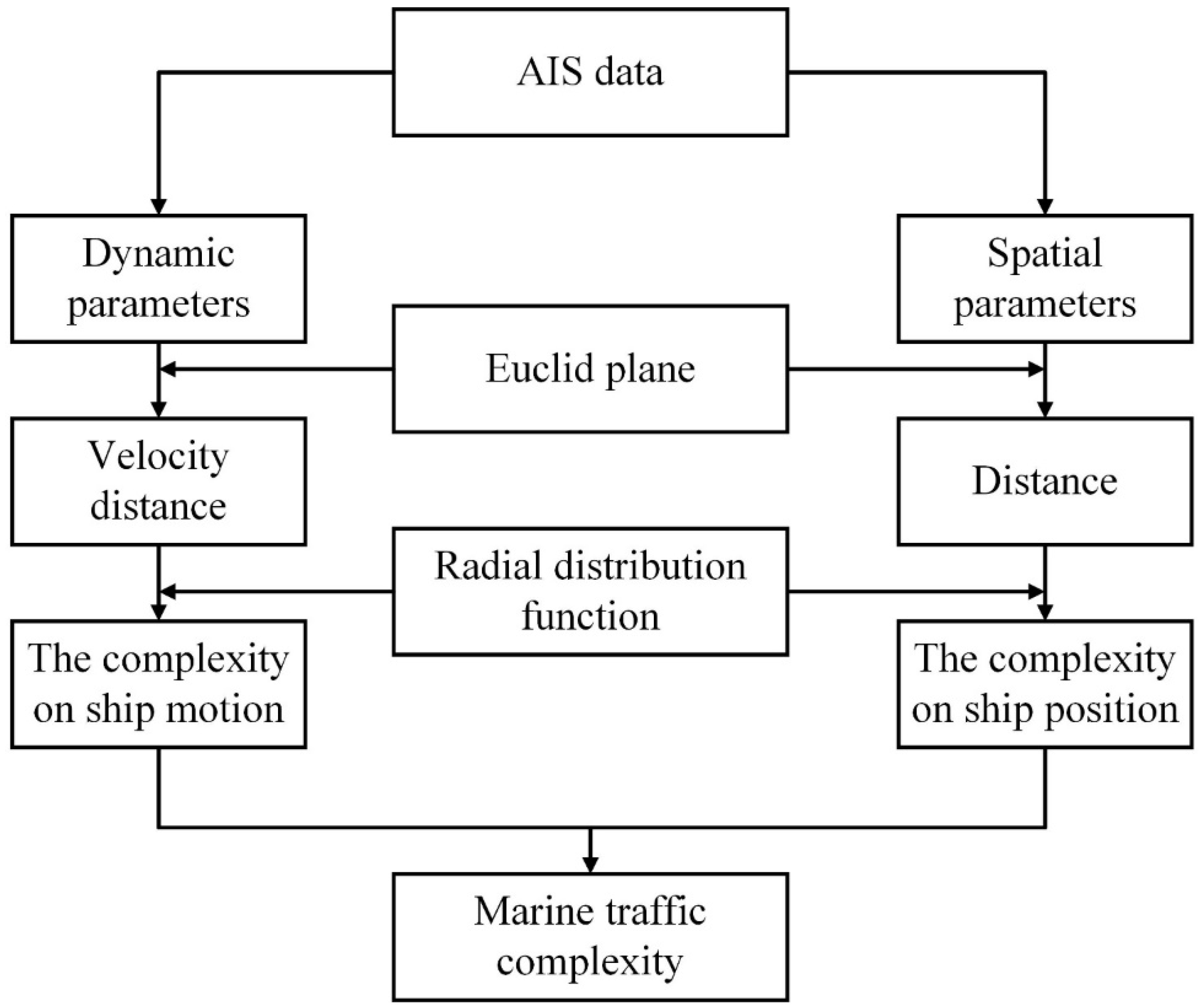
The overall flow chart of the proposed model of marine traffic complexity is shown in Figure 5. The synthesized marine traffic complexity is also a value between 0 and 1, which can represent the complexity level of the ship traffic and can assist marine surveillance operators to better acknowledge, monitor, and organize the marine traffic under complex situations.
3. Case Studies
Some experimental case studies were carried out to validate the proposed marine traffic complexity model. AIS data in Bohai Strait was utilized. Bohai Strait is located between the Bohai Sea and the Northern Yellow Sea in China. The traffic conditions for Bohai Strait provide the model validation with prerequisites. This is because the marine traffic in Bohai Strait is busy and crowded [35], and the traffic volume and traffic density are relatively big, which meansship encounters form much more easily and thus increase the complexity level.
In order to use AIS data for experiments, the AIS source data was first decoded and stored in a database by time sequence. After cleaning and sorting the data, the required information is extracted from the database by Structured Query Languages. In addition, to ensure the information extracted from AIS data can represent the instantaneous scenario accurately, the interpolation process is also conducted.
3.1. Case Studies with Simulated Data
Firstly, some simulated data were used to validate the proposed model. In this case study, the data was simulated on the position, motion, and size parameters of ships. The ships were arranged in the water area where the center is 38.6° N, 120.85° E with a radius of 6 nmile, and this is the location where Laotieshan Precautionary Area locates in reality.
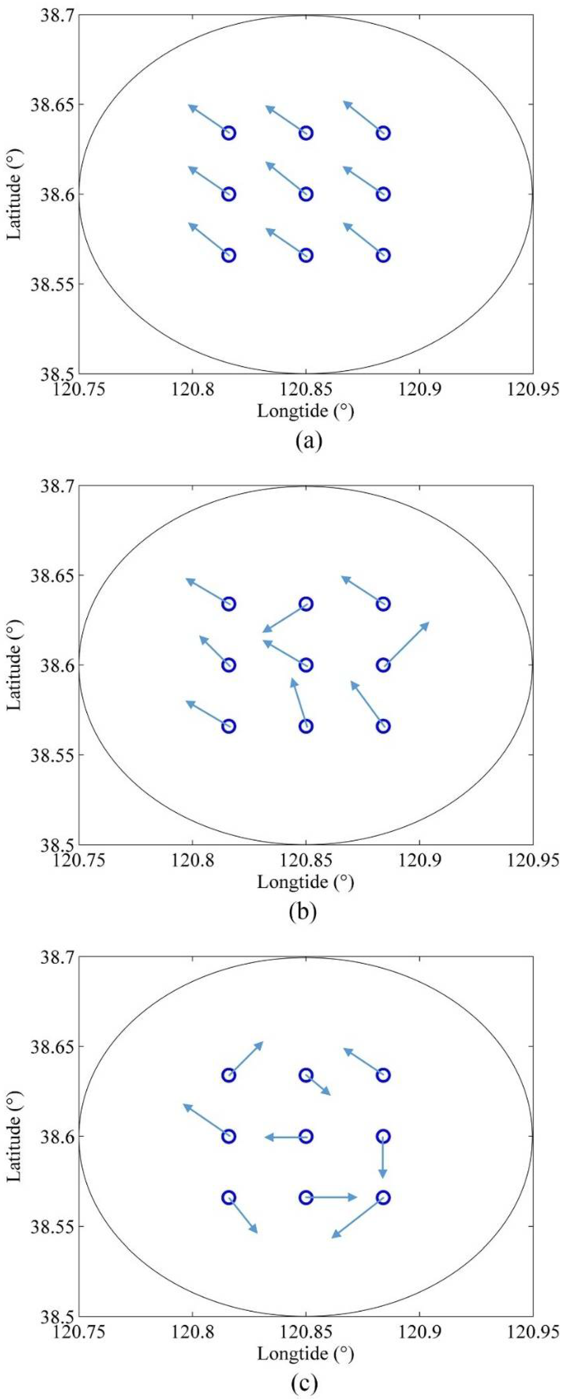
Utilizing the simulated data, three scenarios were formed. The ships in each of these three scenarios were sailing at different velocities, namely, different speeds and courses, but their positions were exactly the same. The three scenarios are shown in Figure 6.
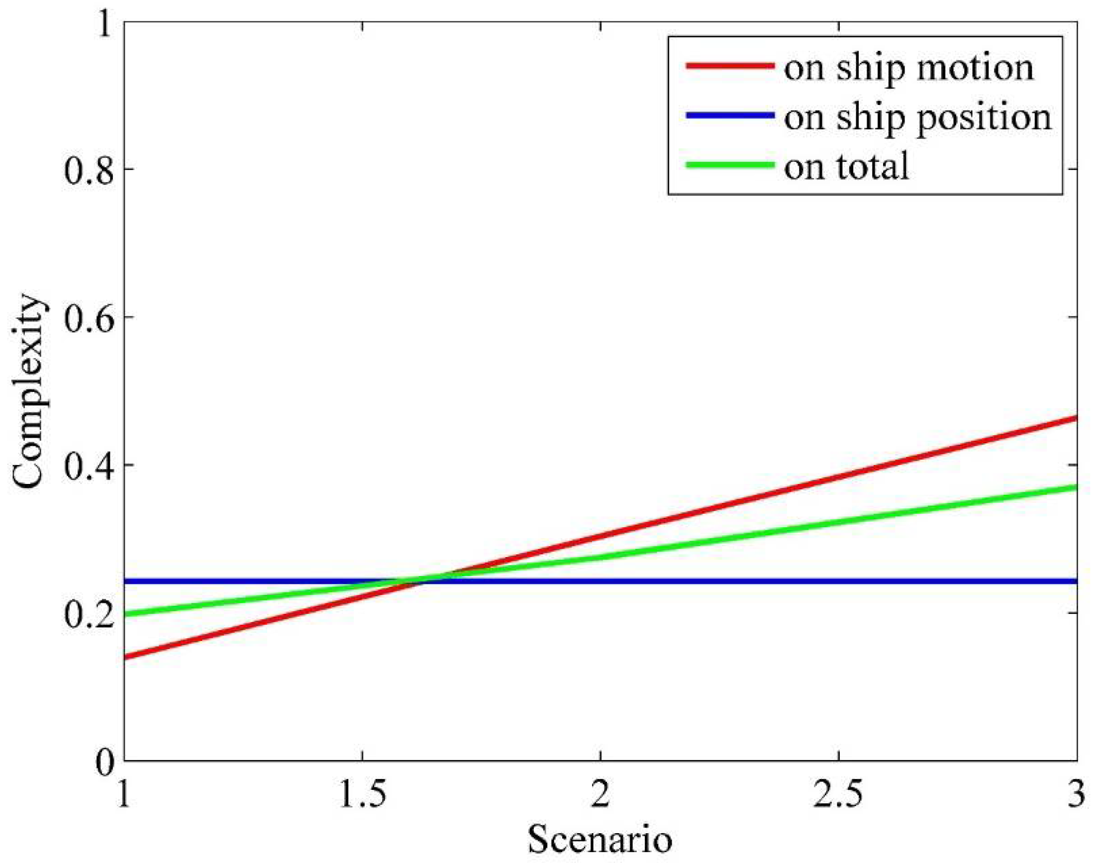
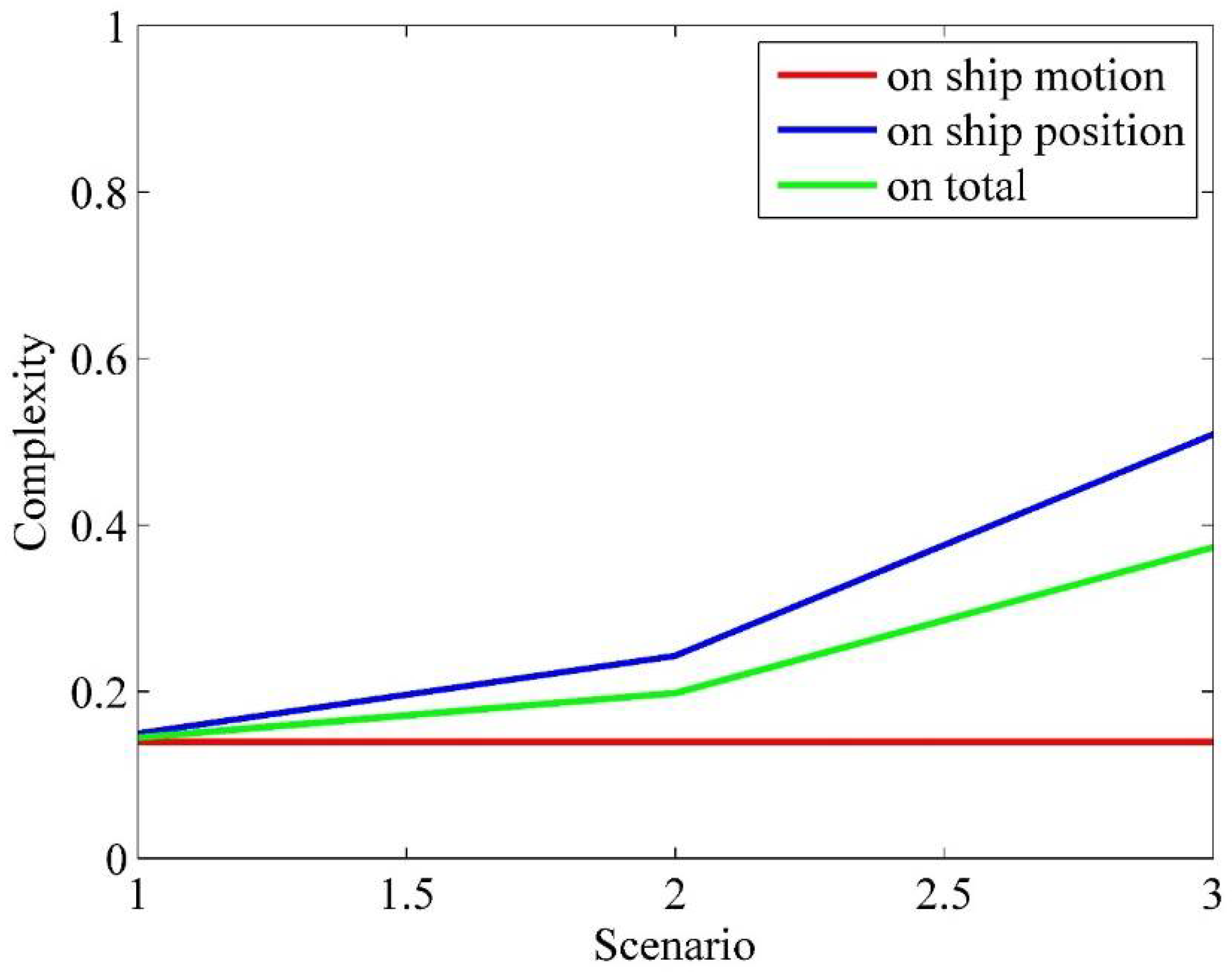
Then, the simulated data of ships was inputted into the proposed model to identify the traffic complexity level of each scenario with related algorithms. The results obtained are shown in Table 1, together with Figure 7.
The results show that the complexity on ship position for each scenario is the same, which is 0.2431, but the complexity on ship motion increases gradually from 0.1397 to 0.4639. The increasing complexity on ship motion makes each scenario’s final marine traffic complexity different, which also increases gradually, from 0.1983 to 0.3703.
In actuality, it can be observed from Figure 6 that the spatial distribution of ship position is exactly the same for each scenario. However, the velocities of ships are not the same. In the first scenario, the velocities for each ship are close, with speeds close to 10 kn, and the courses are close to 300°. However, in the second and third scenarios, the velocities vary obviously, especially in the third scenario. Therefore, the complexity on ship motion, which considers ship speed and course in this article, of these three scenarios should increase gradually, and the complexity on ship position was supposed to be the same, which is confirmed by the results obtained above.
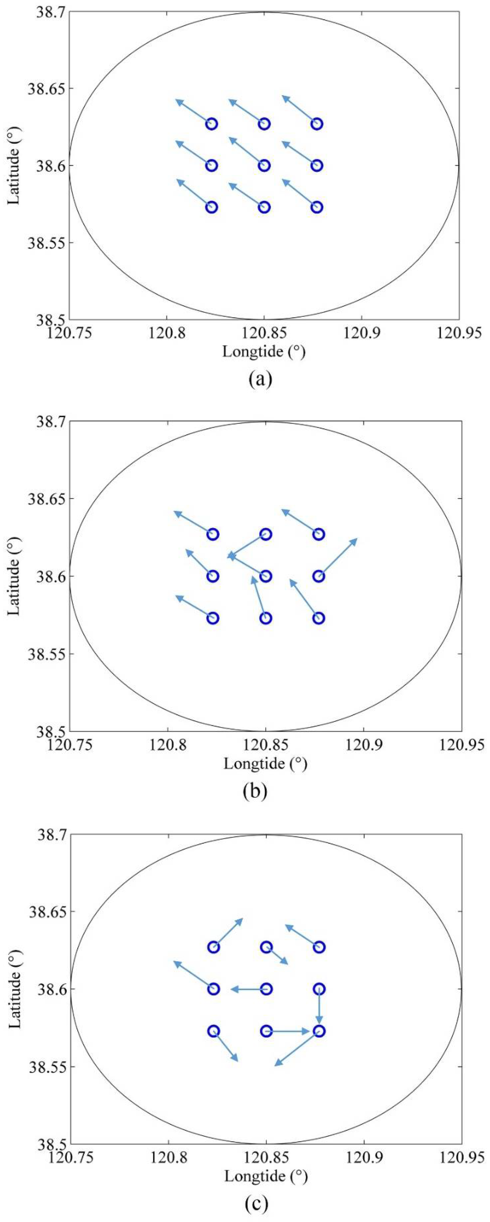
Furtherly, three other scenarios were formed. The ships in each of these three scenarios were sailing at the same velocity, namely the different speeds and courses, but their positions were different. The three scenarios are shown in Figure 8.
Then, the simulated data of ships was inputted the proposed model to calculate the traffic complexity level of each scenario. The results obtained are shown in Table 2, together with Figure 9.
It can be found that the complexity on ship motion for each scenario is the same, which is 0.1397, but the complexity on ship position increases gradually from 0.1496 to 0.5091. The increasing complexity on ship position makes the final marine traffic complexity for each scenario different, which also increases gradually, from 0.1447 to 0.3732.
Actually, it can be observed from Figure 8 that the spatial distribution of ship position is different for each scenario. In the first scenario, the spatial distribution is relatively sparse. In the second and third scenarios, the spatial distribution becomes compact, especially in the third scenario. However, the velocities of ships are exactly the same for each scenario. Therefore, the complexity on ship position, which considers ship position in this article, of these three scenarios should increase gradually, and the complexity on ship motion was supposed to be the same, which is also confirmed by the results obtained above.
3.2. Case Studies with Real AIS Data
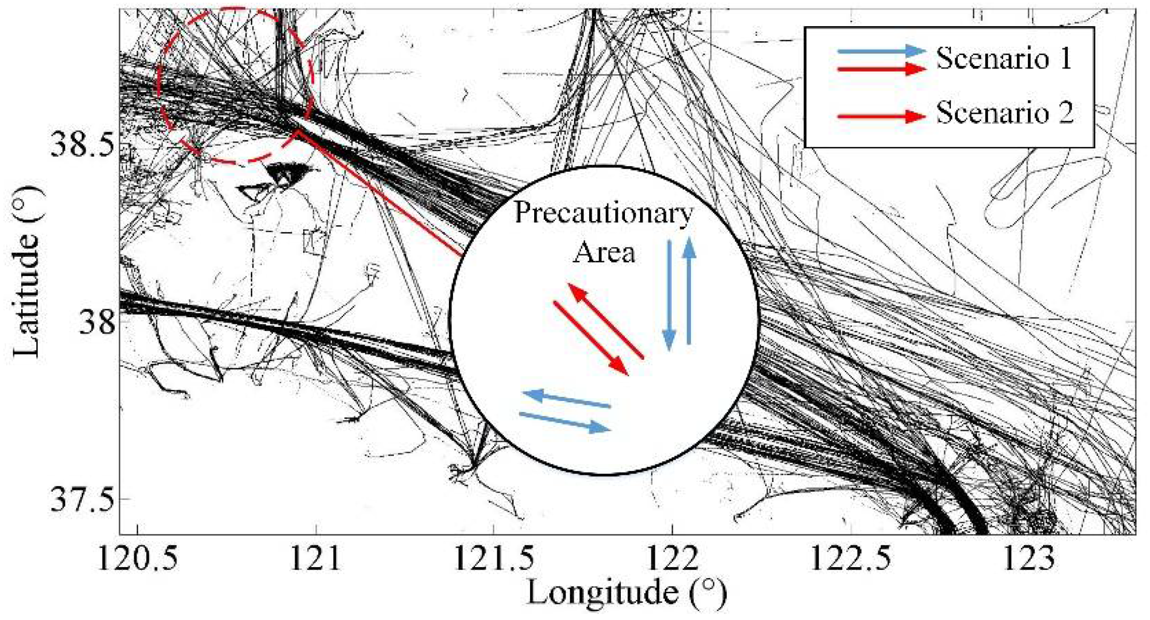
In order to further validate the proposed model, real AIS data was used to carry out some other case studies. The used AIS data was from the ships sailed in the Bohai Strait area. The first case study with real AIS data was to validate the proposed model from a temporal perspective. This case study was carried out in the Laotieshan Precautionary Area (Laotieshan PA), located at the northwest entrance and exit of the Laotieshan Traffic Separation Scheme (Laotieshan TSS). The reason why Laotieshan PA was chosen is the obvious difference between the speed and course, as well as position, of the ships that sailed within it. The traffic in Precautionary Area consists of some different traffic flows, as shown in Figure 10, which makes marine traffic relatively complex in it.
From Figure 10, it can be observed that there are six main traffic flows in Laotieshan PA. Two of them are extended from the direction of Laotieshan TSS. Of the rest four traffic flows, two of them are in the north–south direction, and the other two flows are close to the west–east direction. For this studied area, we divided the traffic into two situations. The first situation is that all traffic flows in PA were considered, which were exhibited as red and blue lines in Figure 10. The second situation is that only the traffic flow which nearly extends the direction of TSS was considered, which is exhibited as red lines in Figure 10.
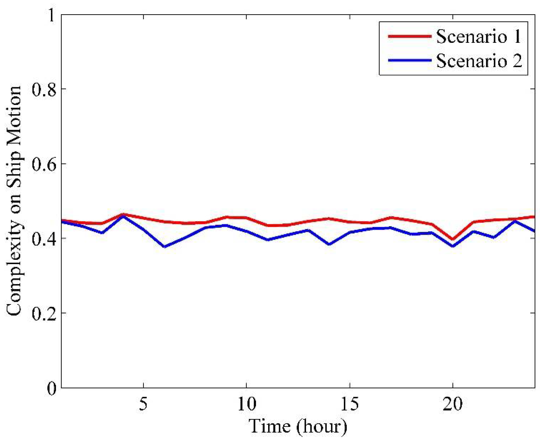
For the two situations, the complexity on ship motion was calculated based on the proposed model. The calculation was conducted for a one-time node for each hour through a day in sequence. The results are shown in Figure 11.
The results show that the complexity on ship motion in the second situation is less than that of the first situation, where the average values are 0.4451 and 0.4169, respectively. The results are consistent with the actual situation. This is because compared with the second situation, there are more different traffic flows considering in the first situation, which makes the speed and course more varied and leads to the increase of complexity level. Therefore, it is proved that the proposed model can identify the marine traffic complexity on ship motion effectively.
In addition, the complexity on ship position for the studied PA was also calculated based on the proposed model. The calculation was conducted for a one-time node for each hour throughout the day. The results are shown in Table 3.
In order to validate that the results are effective in identifying the complexity on ship position. A traditional index was used to make a comparison, which is ship density. According to [5], ship density in a region at time t is the number of ships per unit area in this region at this time, which can be calculated by Equation (16).
where refers to ship density, refers to the number of ships, refers to the time interval and refers to the area of the studied water. For the time nodes in Table 3, ship densities (SD) were calculated, and the results are shown in Table 4.
Then, a Pearson correlation analysis was carried out. The analysis result is shown in Table 5.
It can be found that the p-value was less than 0.01 with a correlation coefficient of 0.692, which indicates that the complexity on ship position and ship density are significantly correlated for all time nodes. As ship density is an index that can reflect the busyness and congestion of marine traffic, we have reason to believe the proposed model can identify the complexity related to a ship position distribution effectively.
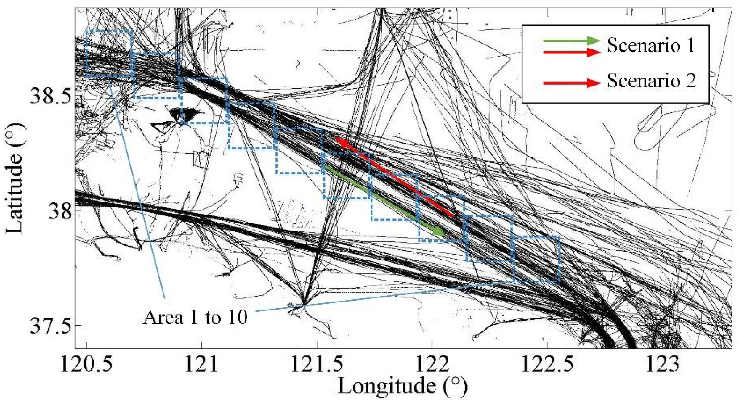
Furthermore, another case study was carried out to validate the proposed model with real AIS data, which was to validate the proposed model from a spatial perspective. In this case study, ten different water areas of the same size were selected. The locations of these ten water areas are shown in Figure 12.
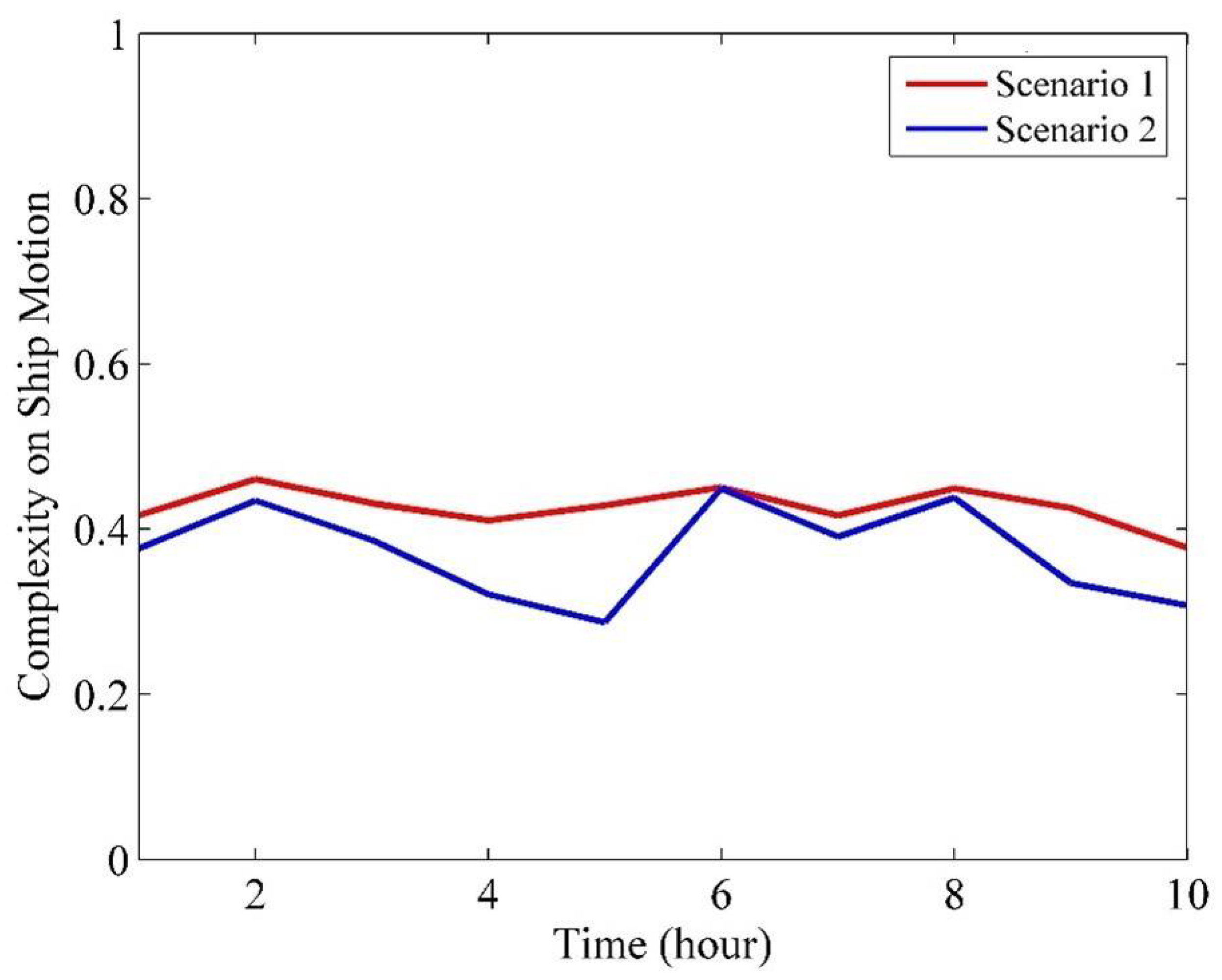
It can be found that the ten water areas are along with the direction of the main traffic flows in Bohai Strait. Firstly, to validate the proposed model can effectively identify the complexity level on ship motion, we also divided the traffic in these areas into two situations. The first situation is that all ships were considered, which is exhibited as the red and green line in Figure 12. The second situation is that only ships sailed to the northwest were considered, exhibited as a red line in Figure 12. For the two situations, the complexity on ship motion was calculated based on the proposed model. The results are shown in Figure 13.
The results show that the complexity on ship motion in the second situation is less than that of the first situation, where the average values are 0.4266 and 0.3725, respectively. The results are consistent with the actual situation because compared with the first situation, only ships heading west were considered, which makes the speed and course less varied and leads to the decrease of complexity level. Therefore, it is proved that the proposed model can identify the marine traffic complexity on ship motion effectively again.
For the complexity on ship position, we also use the index of ship density to evaluate it. The complexity and ship density were calculated, respectively, for the ten studied water areas, and the results are shown in Table 6 and Table 7.
A Pearson correlation analysis was carried out again to examine the correlation between the two sets of values. The analysis result is shown in Table 8.
It can be found that the p-value was less than 0.05 with a correlation coefficient of 0.705, which indicates that the complexity on ship position and ship density are strongly correlated for the ten studied water areas. As mentioned above, since ship density is an index that can reflect the busyness and congestion of marine traffic, we also have a reason to believe the proposed model can identify the complexity related to ship position distribution effectively.
4. Discussion
In this article, a model which can identify the marine traffic complexity was proposed. The proposed model was built with radial distribution function in molecular dynamics. The proposed model consists of two parts, which are the complexity on ship motion and the complexity on ship position, respectively. In identifying the complexity on ship motion, the speed and course of the ship were considered by constructing a two-dimension velocity plane. The velocity distance in the velocity plane was treated as the distance in the radial distribution function model. In identifying the complexity on ship position, the position of the ship was considered by constructing a traditional two-dimensional Euclidean plane. The final marine traffic complexity can be obtained by merging these two complexities. The proposed model can evaluate marine traffic complexity from an objective perspective utilizing the ship attributes extracted from AIS data. It can assist maritime surveillance operators in acknowledging the marine traffic situation in the jurisdiction water area in a more objective way, especially under complex traffic scenarios, where they may face a cognization difficult only by their subjective judgment. It can also facilitate their services for ships and traffic and thus contribute to the enhancement of marine traffic safety.
For validating the proposed model, a series of experimental case studies were carried out. At first, in Section 3.1, two simulated case studies were conducted. As the proposed model consists of two parts, which are the complexity on ship motion and ship position, we validate the two complexities, respectively, by controlling the variables in each simulated case study. In the first simulated case study, we made the ship positions fixed and changed the ship velocities gradually by changing the ship speeds and courses from an ordered state to a disordered state. The complexity on ship motion part in the proposed model can effectively react to this change. In the Second simulated case study, we fixed the ship velocities but changed the ship position gradually to make them more and more compact. The complexity on ship position part in the proposed model can effectively react to this change. The results can prove the effectiveness of the proposed model to some extent. Furthermore, in Section 3.2, two case studies with real AIS data were carried out to validate the proposed model. The proposed model was proved in temporal and spatial perspectives, respectively. For the validation from a temporal perspective, Laotieshan PA was chosen as the studied water area. Two situations of marine traffic in Laotieshan PA were divided, one considers all traffic and the other only considers limited traffic flows. For the two situations, 24 time nodes were selected from each hour through the day, and we calculated the complexity on ship motion for these time nodes. The results show that the complexity of the situation of limited traffic is less than that of the situation of all traffic, which conforms to reality. For the complexity on ship position, we also calculated the results for all time nodes. To evaluate its effectiveness, the ship density index, which can reflect the busyness and congestion of the ship was adopted. A Pearson correlation analysis between the ship density index and the complexity on ship position was conducted. The result shows a significant correlation between them, thus verifying the effectiveness of the results to some extent. In addition, to validate the effectiveness of the proposed model more sufficiently, a case study from a spatial perspective was carried out. Ten water areas were treated as studied areas. For the traffic in the studied area, we also divided it into two situations; one considers all traffic, and the other only considers nearly one-way traffic. Then, the complexity on ship motion was calculated. The results obtained by the proposed model can still react to the change in the situation, which can exhibit that the value of a limited traffic situation is less than that of a full traffic situation. Moreover, we identified the complexity on ship position for the ten studied areas and used ship density as an evaluating index again. The Pearson correlation analysis result shows that there exists a strong correlation between them, thus proving the effectiveness of the results again.
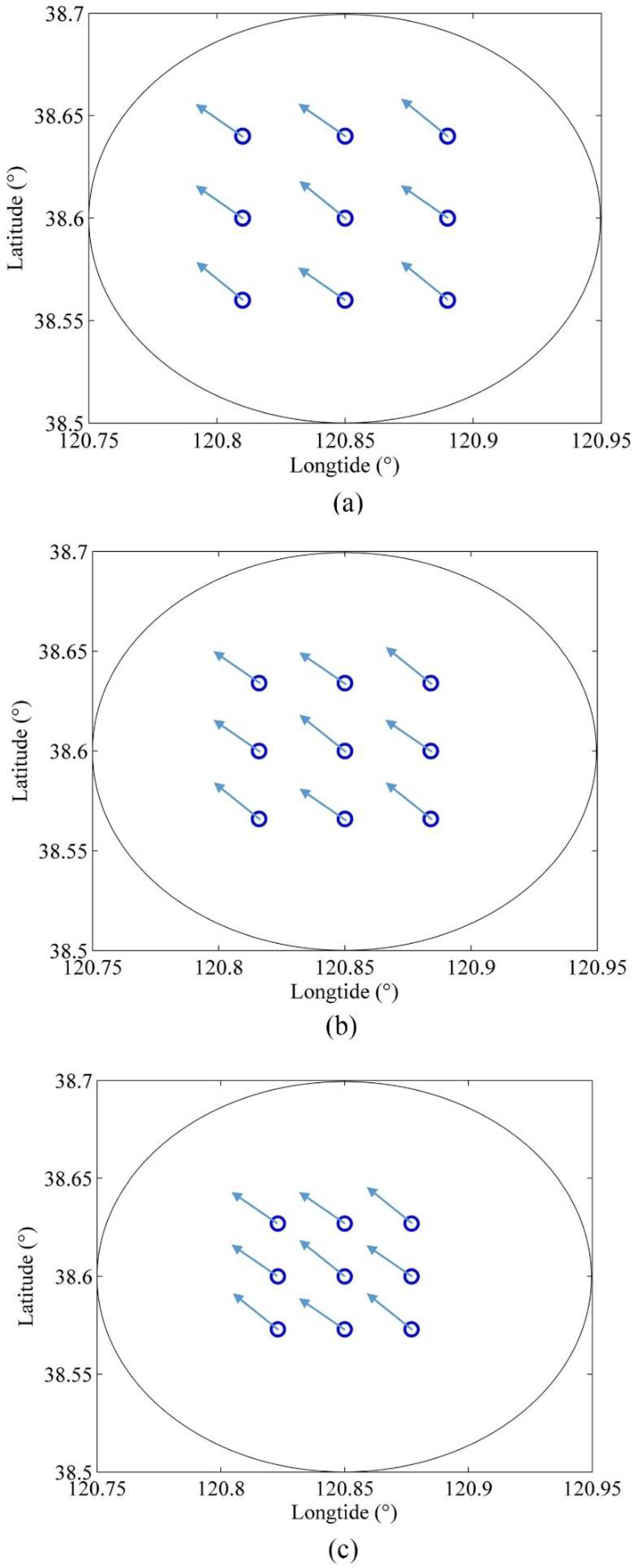
RDF was used to model the ship density and traffic density in [23]. As mentioned in that article, the model can reveal the traffic complexity to some extent. However, the RDF model in [23] can only evaluate the complexity from a spatial distribution perspective; the ship position is the only considered factor. However, ship motion is also important for determining traffic complexity. If the ship speeds and courses were varied and disordered, the encounter between ships may form easier, and thus increase the difficulties for collision avoidance. Under such complex traffic situations, collision accidents are more likely to happen. Therefore, in order to sufficiently reflect the traffic complexity level, only considering ship positions is not enough. In order to prove this, we carried out two sets of case studies in Section 3.1. It can be observed from Figure 6, Figure 7, and Table 1 that when ship positions were fixed, only evaluating the complexity on ship position cannot distinguish the difference between the three scenarios. For distinguishing the complexity levels between them, the complexity on ship motion is supposed to be calculated at the same time. In order to prove the advantage of the proposed model compared to the previous model further, the case study in Section 3.1 was expanded here. The compactness of the ships in Figure 6 is moderate. Here, we changed the ship position distribution to a more compact state, as shown in Figure 14. The complexity results calculated based on the proposed model are shown in Table 9.
It can be found that the complexity on ship position in Table 9 can react to the change of compactness, which becomes higher compared to the results in Table 2. However, for the three scenarios in Figure 14, it can be observed that the ship motions are obviously different. However, the complexity on ship position cannot distinguish them, which can only be performed by calculating the complexity on ship motion in the proposed model at the same time. Therefore, the results illustrate the advantage of the proposed model in fully evaluating marine traffic complexity again compared to the previous model.
In addition, the ship density index was used to evaluate the complexity on ship position in Section 3.2, but it should be noted that the ship density is not able to fully reflect the complexity too. Take the scenarios (a) in Figure 6 and Figure 14 as an example, it can be found that the ships become more compact, but their density remains the same, which is both for time period. However, the proposed model can react to this change in ship compactness, increasing from 0.2431 to 0.5091. Therefore, the proposed model also has the advantage of identifying complexity compared with the traditional ship density index.
However, there are also some limitations to the proposed model in this article. Firstly, in modeling dynamic traffic complexity, the speed and course are considered because they are the most important dynamic parameters for ships. However, apart from speed and course, there are some other parameters that may influence traffic complexity, such as rate of turn, encountering angle, encountering type, and changing rate of speed. For example, encountering type includes head-on, crossing, and overtaking; different encountering type may cause different traffic complexity according to a different type of waterway. The relationship between traffic complexity and the factors mentioned above needs to be studied further in the future. Additionally, the proposed model calculates marine traffic complexity by using AIS data. Although AIS is mandatory on most of the ships, there are still some small ships that do not fit AIS, such as fishing ships. Therefore, for the waterway off the coast, where fishing ships may appear, as AIS data is not capable of covering such ships, the results may not be accurate enough to represent the actual traffic complexity in the waterway. To solve this problem, some other data should be used in modeling marine traffic complexity, such as Radar data or traffic observation data. Moreover, the newest AIS data was needed to further validate the model under the current traffic situation. In addition, in synthesizing the two complexities in a final marine traffic complexity, the expression and method in [32,33,34] were adopted. Considering that the studied area is relatively open, the two coefficients are taken as the same value in case studies. However, for different kinds of water, the two coefficients may be changed, or maritime surveillance can determine the coefficient according to their own purpose. The relationship between the coefficients and the kinds of water is supposed to be studied in the future.
5. Conclusions
Herein, a marine traffic complexity model considering the motion and density of the ship was proposed, which can identify the complexity level of marine traffic in a waterway. To establish the proposed model, the radial distribution function in molecular dynamics was used. Firstly, ship traffic was converted to a ship particle system where ships were converted to ship particles. Then, the complexity on ship motion and ship position were modeled, respectively, by analyzing the radial distribution of ships’ dynamic and spatial parameters in a Euclid plane. Finally, the two complexities were merged to obtain the marine traffic complexity by an analytical method. In order to validate the proposed model, some experimental case studies were conducted in Bohai Strait waters with real AIS data and simulated data. The results show that the proposed model can effectively and accurately identify the marine traffic complexity in a waterway, react to the change of variable, and has the advantage compared with the previous model and the traditional density index in identifying complexity level. In addition, by utilizing the proposed model, marine surveillance operators can better acknowledge, monitor, and organize the traffic under complex situations, so as to improve marine traffic safety.
The proposed model also has some limitations which should be improved in future research. Firstly, apart from speed and course, some other dynamic parameters which may influence the traffic complexity, such as rate of turn, encountering angle, encountering type, and changing rate of speed, were not considered. The relationship between traffic complexity and the factors mentioned above needs to be studied further in the future. Secondly, as AIS data is not available for some small ships, such as fishing ships, the results may not be accurate enough to represent the traffic complexity, including such ships in the waterway. Therefore, some other types of data should be used in modeling marine traffic complexity. Thirdly, the merging of the two complexities in this article is under simple consideration; the relationship between the coefficients and the water types should be explored further in future research.
Author Contributions
Conceptualization, Z.L.; methodology, Z.L.; software, Z.L.; validation, Z.L., X.Y.; formal analysis, Z.L.; investigation, Z.L.; resources, Z.W. and Z.Z.; data curation, Z.L.; writing—original draft preparation, Z.L.; writing—review and editing, Z.L., Z.W., and Z.Z.; visualization, Z.L.; supervision, Z.W. and Z.Z.; project administration, Z.L.; funding acquisition, Z.L. All authors have read and agreed to the published version of the manuscript.
Funding
This research was funded by “the Fundamental Research Funds for the Central Universities” (Grant. 3132022134) and the Talent Research Start-up Funds of Dalian Maritime University (Grant. 02500128).
Institutional Review Board Statement
Not applicable.
Informed Consent Statement
Not applicable.
Data Availability Statement
Not applicable.
Acknowledgments
We would like to express our gratitude to the editors and reviewers whose valuable comments and suggestions will make improvements to the quality of this paper.
Conflicts of Interest
The authors declare no conflict of interest.
References
- Weng, J.; Liao, S.; Wu, B.; Yang, D. Exploring effects of ship traffic characteristics and environmental conditions on ship collision frequency. Marit. Policy Manag. 2020, 47, 523–543. [Google Scholar] [CrossRef]
- Zhen, R.; Shi, Z.; Liu, J.; Shao, Z. A novel arena-based regional collision risk assessment method of multi-ship encounter situation in complex waters. Ocean Eng. 2022, 246, 110531. [Google Scholar] [CrossRef]
- Tu, E.; Zhang, G.; Rachmawati, L.; Rajabally, E.; Huang, G. Exploiting AIS Data for Intelligent Maritime Navigation: A Comprehensive Survey From Data to Methodology. IEEE Trans. Intell. Transp. Syst. 2018, 19, 1559–1582. [Google Scholar] [CrossRef]
- Silveira, P.A.M.; Teixeira, A.P.; Guedes Soares, C. Use of AIS data to characterize marine traffic patterns and ship collision risk off the coast of Portugal. J. Navig. 2013, 66, 879–898. [Google Scholar] [CrossRef] [Green Version]
- Wu, L.; Xu, Y.; Wang, Q.; Wang, F.; Xu, J. Mapping Global Shipping Density from AIS Data. J. Navig. 2017, 70, 67–81. [Google Scholar] [CrossRef]
- Yu, H.; Fang, Z.; Murray, A.T.; Peng, G. A direction-constrained space-time prism-based approach for quantifying possible multi-ship collision risks. IEEE Trans. Intell. Transp. Syst. 2019, 22, 131–141. [Google Scholar] [CrossRef]
- Zhang, W.; Feng, X.; Goerlandt, F.; Liu, Q. Towards a Convolutional Neural Network model for classifying regional ship collision risk levels for waterway risk analysis. Reliab. Eng. Syst. Saf. 2020, 204, 107127. [Google Scholar] [CrossRef]
- Bakdi, A.; Glad, I.K.; Vanem, E.; Engelhardtsen, Ø. AIS-based multiple vessel collision and grounding risk identification based on adaptive safety domain. J. Mar. Sci. Eng. 2020, 8, 5. [Google Scholar] [CrossRef] [Green Version]
- Wen, Y.; Huang, Y.; Zhou, C.; Yang, J.; Xiao, C.; Wu, X. Modelling of marine traffic flow complexity. Ocean Eng. 2015, 104, 500–510. [Google Scholar] [CrossRef]
- Rong, H.; Teixeira, A.; Guedes Soares, C. Data mining approach to shipping route characterization and anomaly detection based on AIS data. Ocean Eng. 2020, 198, 106936. [Google Scholar] [CrossRef]
- Zhang, J.; Wan, C.; He, A.; Zhang, D.; Guedes Soares, C. A two-stage black-spot identification model for inland waterway transportation. Reliab. Eng. Sys. Saf. 2021, 213, 107677. [Google Scholar] [CrossRef]
- Liu, D.; Wang, X.; Cai, Y.; Liu, Z.; Liu, Z. A Novel Framework of Real-Time Regional Collision Risk Prediction Based on the RNN Approach. J. Mar. Sci. Eng. 2020, 8, 224. [Google Scholar] [CrossRef] [Green Version]
- Liu, Z.; Wu, Z.; Zheng, Z. An Improved Danger Sector Model for Identifying the Collision Risk of Encountering Ships. J. Mar. Sci. Eng. 2020, 8, 609. [Google Scholar] [CrossRef]
- Zhen, R.; Shi, Z.; Shao, Z.; Liu, J. A novel regional collision risk assessment method considering aggregation density under multi-ship encounter situations. J. Navig. 2022, 75, 76–94. [Google Scholar] [CrossRef]
- Yu, Q.; Teixeira, A.P.; Liu, K.; Guedes Soares, C. Framework and application of multi-criteria ship collision risk assessment. Ocean Eng. 2022, 250, 111006. [Google Scholar] [CrossRef]
- Merrick, J.R.W.; van Dorp, J.R.; Blackford, J.P.; Shaw, G.L.; Harrald, J.; Mazzuchi, T.A. A traffic density analysis of proposed ferry service expansion in San Francisco Bay using a maritime simulation model. Reliab. Eng. Syst. Saf. 2003, 81, 119–132. [Google Scholar] [CrossRef]
- Altan, Y.C.; Otay, E.N. Maritime Traffic Analysis of the Strait of Istanbul based on AIS data. J. Navig. 2017, 70, 1367–1382. [Google Scholar] [CrossRef]
- Ramin, A.; Mustaffa, M.; Ahmad, S. Prediction of Marine Traffic Density Using Different Time Series Model From AIS data of Port Klang and Straits of Malacca. Trans. Marit. Sci. 2020, 9, 217–223. [Google Scholar] [CrossRef]
- Kang, L.; Meng, Q.; Liu, Q. Fundamental diagram of ship traffic in the Singapore Strait. Ocean Eng. 2018, 147, 340–354. [Google Scholar] [CrossRef]
- van Westrenen, F.; Ellerbroek, J. The effect of traffic complexity on the development of near misses on the North Sea. IEEE Trans. Syst. Man Cyber. Syst. 2015, 47, 432–440. [Google Scholar] [CrossRef]
- Du, L.; Valdez Banda, O.A.; Goerlandt, F.; Kujala, P.; Zhang, W. Improving Near Miss Detection in Maritime Traffic in the Northern Baltic Sea from AIS Data. J. Mar. Sci. Eng. 2021, 9, 180. [Google Scholar] [CrossRef]
- Endrina, N.; Rasero, J.C.; Konovessis, D. Risk analysis for RoPax vessels: A case of study for the Strait of Gibraltar. Ocean Eng. 2018, 151, 141–151. [Google Scholar] [CrossRef]
- Liu, Z.; Wu, Z.; Zheng, Z. Modelling ship density using a molecular dynamics approach. J. Navig. 2020, 73, 628–645. [Google Scholar] [CrossRef]
- Widom, B. Statistical Mechanics A Concise Introduction for Chemists; Cambridge University Press: Cambridge, UK, 2002; p. 102. [Google Scholar]
- McQuarrie, D.A. Statistical Mechanics; HARPER & ROW: New York, NY, USA, 1976; pp. 254–260. [Google Scholar]
- IUPAC. Compendium of Chemical Terminology: IUPAC Recommendations; Blackwell Scientific Publications: Hoboken, NJ, USA, 1987; p. 335. [Google Scholar]
- Bauer, R.C.; Birk, J.P.; Marks, P. Introduction to Chemistry: A Conceptual Approach; McGraw-Hill Inc.: New York, NY, USA, 2009; pp. 403–405. [Google Scholar]
- Ma, X.; He, J.; Xie, X.; Zhu, J.; Ma, B. Study of C-S-H gel and C-A-S-H gel based on molecular dynamics simulation. Concrete 2019, 351, 118–122. (In Chinese) [Google Scholar]
- Chandler, D. Introduction to Modern Statistical Mechanics; Oxford University Press: Oxford, UK, 1987; pp. 199–200. [Google Scholar]
- Zhen, R.; Riveiro, M.; Jin, Y. A novel analytic framework of real-time multi-vessel collision risk assessment for maritime traffic surveillance. Ocean Eng. 2017, 145, 492–501. [Google Scholar] [CrossRef]
- Fujii, Y.; Tanaka, K. Traffic capacity. J. Navig. 1971, 24, 543–552. [Google Scholar] [CrossRef]
- Kearon, J. Computer program for collision avoidance and track keeping. In Proceedings of the International Conference on Mathematics Aspects of Marine Traffic, London, UK, 1 September 1977. [Google Scholar]
- Lisowski, J. Determining the optimal ship trajectory in collision situation. In Proceedings of the IX International Scientific and Technical Conference on Marine Traffic Engineering, Szczecin, Poland, 19–22 October 2001. [Google Scholar]
- Szlapczynski, R. A unified measure of collision risk derived from the concept of a ship domain. J. Navig. 2006, 59, 477–490. [Google Scholar] [CrossRef]
- Liu, J.; Han, X. Survey and Analysis of Vessel Traffic Flow in the Bohai Strait. Ship Ocean Eng. 2008, 37, 95–98. (In Chinese) [Google Scholar]
Figure 1.
An example radial distribution of a particle system.

Figure 2.
The ship molecules and ship traffic particle system.

Figure 3.
The velocity plane of ship traffic particle system.

Figure 4.
An example radial distribution graph of ship velocity.

Figure 5.
The flow chart of the proposed model.

Figure 6.
The three scenarios for the first simulated case study (a) Scenario 1; (b) Scenario 2; (c) Scenario 3.
Figure 6.
The three scenarios for the first simulated case study (a) Scenario 1; (b) Scenario 2; (c) Scenario 3.

Figure 7.
The results of the first simulated case study.

Figure 8.
The three scenarios for the second simulated case study (a) Scenario 1; (b) Scenario 2; (c) Scenario 3.
Figure 8.
The three scenarios for the second simulated case study (a) Scenario 1; (b) Scenario 2; (c) Scenario 3.

Figure 9.
The results of the second simulated case study.

Figure 10.
The location of Laotieshan PA and its main traffic flows.

Figure 11.
The comparison between the complexity on ship motion for the two situations.

Figure 12.
The locations of these ten water areas.

Figure 13.
The complexity on ship motion for the spatial case study.

Figure 14.
The scenarios for the expanded case study (a) Scenario 1; (b) Scenario 2; (c) Scenario 3.
Figure 14.
The scenarios for the expanded case study (a) Scenario 1; (b) Scenario 2; (c) Scenario 3.


Table 1.
The results of the first simulated case study.
| Scenario | Scenario 1 | Scenario 2 | Scenario 3 |
|---|---|---|---|
| Complexity on ship motion | 0.1397 | 0.3037 | 0.4639 |
| Complexity on ship position | 0.2431 | 0.2431 | 0.2431 |
| Marine traffic complexity | 0.1983 | 0.2751 | 0.3703 |
Table 2.
The results of the second simulated case study.
| Scenario | Scenario 1 | Scenario 2 | Scenario 3 |
|---|---|---|---|
| Complexity on ship motion | 0.1397 | 0.1397 | 0.1397 |
| Complexity on ship position | 0.1496 | 0.2431 | 0.5091 |
| Marine traffic complexity | 0.1447 | 0.1983 | 0.3733 |
Table 3.
The complexity on ship position for the studied PA.
| Time | |
|---|---|
| 0–1 | 0.1855 |
| 1–2 | 0.0973 |
| 2–3 | 0.0932 |
| 3–4 | 0.0926 |
| 4–5 | 0.0585 |
| 5–6 | 0.0656 |
| 6–7 | 0.0748 |
| 7–8 | 0.0608 |
| 8–9 | 0.1106 |
| 9–10 | 0.1190 |
| 10–11 | 0.1174 |
| 11–12 | 0.1053 |
| 12–13 | 0.1589 |
| 13–14 | 0.1282 |
| 14–15 | 0.2052 |
| 15–16 | 0.1630 |
| 16–17 | 0.0943 |
| 17–18 | 0.1375 |
| 18–19 | 0.1277 |
| 19–20 | 0.0965 |
| 20–21 | 0.1382 |
| 21–22 | 0.1339 |
| 22–23 | 0.1498 |
| 23–24 | 0.1143 |
Table 4.
The ship density for the studied PA.
| Time | |
|---|---|
| 0–1 | 0.0796 |
| 1–2 | 0.0707 |
| 2–3 | 0.0707 |
| 3–4 | 0.0619 |
| 4–5 | 0.0442 |
| 5–6 | 0.0619 |
| 6–7 | 0.0442 |
| 7–8 | 0.0442 |
| 8–9 | 0.0707 |
| 9–10 | 0.0973 |
| 10–11 | 0.0796 |
| 11–12 | 0.0619 |
| 12–13 | 0.0973 |
| 13–14 | 0.0707 |
| 14–15 | 0.1326 |
| 15–16 | 0.0707 |
| 16–17 | 0.0973 |
| 17–18 | 0.0707 |
| 18–19 | 0.0707 |
| 19–20 | 0.0796 |
| 20–21 | 0.0884 |
| 21–22 | 0.0619 |
| 22–23 | 0.0796 |
| 23–24 | 0.0884 |
Unit of SD:
Table 5.
Pearson correlation analysis between and SD for 24 time nodes.
| p Value | Correlation Coefficient |
|---|---|
| <0.01 | 0.692 |
Table 6.
The complexity on ship position for the ten studied water areas.
| Area | |
|---|---|
| 1 | 0.0855 |
| 2 | 0.1051 |
| 3 | 0.1897 |
| 4 | 0.0927 |
| 5 | 0.1054 |
| 6 | 0.1247 |
| 7 | 0.0902 |
| 8 | 0.0563 |
| 9 | 0.0769 |
| 10 | 0.1310 |
Table 7.
The ship density for the ten studied water areas.
| Area | |
|---|---|
| 1 | 0.0354 |
| 2 | 0.0884 |
| 3 | 0.1238 |
| 4 | 0.0973 |
| 5 | 0.0442 |
| 6 | 0.1149 |
| 7 | 0.0973 |
| 8 | 0.0531 |
| 9 | 0.0531 |
| 10 | 0.0973 |
Table 8.
Pearson correlation analysis between and SD for the ten studied water areas.
| p-Value | Correlation Coefficient |
|---|---|
| <0.05 | 0.705 |
Unit of SD:
Table 9.
The results of the expanded case study.
| Scenario | Scenario 1 | Scenario 2 | Scenario 3 |
|---|---|---|---|
| Complexity on ship motion | 0.1397 | 0.3037 | 0.4639 |
| Complexity on ship position | 0.5091 | 0.5091 | 0.5091 |
| Marine traffic complexity | 0.3733 | 0.4192 | 0.4870 |
Publisher’s Note: MDPI stays neutral with regard to jurisdictional claims in published maps and institutional affiliations. |
© 2022 by the authors. Licensee MDPI, Basel, Switzerland. This article is an open access article distributed under the terms and conditions of the Creative Commons Attribution (CC BY) license (https://creativecommons.org/licenses/by/4.0/).
Share and Cite
MDPI and ACS Style
Liu, Z.; Wu, Z.; Zheng, Z.; Yu, X. A Molecular Dynamics Approach to Identify the Marine Traffic Complexity in a Waterway. J. Mar. Sci. Eng. 2022, 10, 1678. https://doi.org/10.3390/jmse10111678
AMA Style
Liu Z, Wu Z, Zheng Z, Yu X. A Molecular Dynamics Approach to Identify the Marine Traffic Complexity in a Waterway. Journal of Marine Science and Engineering. 2022; 10(11):1678. https://doi.org/10.3390/jmse10111678
Chicago/Turabian StyleLiu, Zihao, Zhaolin Wu, Zhongyi Zheng, and Xianda Yu. 2022. "A Molecular Dynamics Approach to Identify the Marine Traffic Complexity in a Waterway" Journal of Marine Science and Engineering 10, no. 11: 1678. https://doi.org/10.3390/jmse10111678
Note that from the first issue of 2016, this journal uses article numbers instead of page numbers. See further details here.