Turbulent Eddy Generation for the CFD Analysis of Hydrokinetic Turbines

Abstract

This paper presents a novel theoretical and computational methodology for the generation of an onset turbulent field with prescribed properties in the numerical simulation of an arbitrary viscous flow. The methodology is based on the definition of a suitable distribution of volume force terms in the right-hand side of the Navier–Stokes equations. The distribution is represented by harmonic functions that are randomly variable in time and space. The intensity of the distribution is controlled by a simple PID strategy in order to obtain that the generated turbulent flow matches a prescribed turbulence intensity. A further condition is that a homogeneous isotropic flow is established downstream of the region where volume force terms are imposed. Although it is general, the proposed methodology is primarily intended for the computational modelling of hydrokinetic turbines in turbulent flows representative of tidal or riverine installations. A first numerical application is presented by considering the injection of homogeneous and isotropic turbulence with 16% intensity into a uniform unbounded flow. The analysis of statistical properties as auto-correlation, power spectral density, probability density functions, demonstrates that the generated flow tends to achieve satisfactory levels of stationarity and isotropy, whereas the simple control strategy used determines underestimated turbulent intensity levels.

1. Introduction

The hydrodynamic interaction between a fluid and a solid body moving through it is largely affected by the turbulence of the flow incoming to the body. By a simple observation, the turbulent nature of a flow is revealed by eddies with variable extension (length scale) and characteristic period (time scale). In terms of flow velocity, the eddies are responsible for a fluctuating component that can be assumed to perturb an onset smooth (laminar) flow. In contrast to the laminar flow that has a deterministic behaviour, turbulent fluctuations have a random nature.

Dealing with marine engineering problems, the impact of onset flow turbulence is of primary importance in the hydrodynamics of surface and underwater vehicles and of offshore structures. Typical examples for rotary-wing systems are the propellers that operate in the turbulent wake shed by the ship hull [1] or hydrokinetic turbines immersed in a tidal stream [2,3]. In both cases, three main aspects of the interaction between rotating blades and the onset turbulent flow can be identified. Random fluctuations of the onset flow provoke the destabilization of the laminar boundary layer on the blade surface, and trigger the transition to turbulent boundary layer, which results into increased drag. Next, turbulent eddies with length and time scales compatible with rotor size and rotational speed, are responsible for the generation of fluctuating loads on rotor blades, with harmful effects in terms of vibrations and fatigue [4,5,6]. Not less important, the evolution of the wake shed by rotor blades is largely affected by the intensity of the onset turbulent flow, with direct consequences on the performance of rotors operating in the wake of other rotors, as in the case of arrays of turbines [7].

Considering energy harvesting systems, an intrinsic problem lies in the difficulty to characterize the complexity of the turbulent stream in a tidal site [8,9]. A variety of approaches exist in the literature on the modelling of onset flow turbulence in the Computational Fluid Dynamics (CFD) analysis of hydrokinetic turbines. Common to these methodologies is to develop computationally efficient approaches to generate a randomly fluctuating velocity field that interacts with the rest of the solution. A key difficulty is to obtain a simulated turbulent field with characteristics that are representative of real-life tidal flows. A recent review on the subject is proposed in [10]. Computational models for the generation of onset turbulent flows can be grouped into two main classes, precursor methods and synthetic methods. In the first case, a turbulent velocity field is injected into the computational domain by using experimental data or results from separate CFD modelling, notably by a DNS (Direct Navier–Stokes) solution. In the latter case, a suitable computational model is integrated into the CFD model in order to generate a flow velocity perturbation that satisfies statistical properties that are consistent with natural turbulent flows. The methodology proposed in the present work falls within the broad class of synthetic methods. The turbulence generation model is intended for integration into a general purpose Navier–Stokes solver. The production of turbulent eddies is obtained through a volume force distribution defined as the combination of a harmonic distribution and a contribution that is randomly variable in time and space. The volume force terms are distributed in a narrow region of the computational domain, and the generated turbulent structures are shed downstream by the flow. Volume force modelling applied here grounds on authors’ experience in the use of this type of methodology in the development of hybrid viscous/inviscid flow solvers for applications to ship propulsion [11] and tidal turbines [12,13]. In order to match imposed values of flow turbulence, the intensity of volume force terms is iteratively updated by a suitable control strategy. The variance of the flow velocity components are taken as quantities observed by the control algorithm. In the present study, a simple Proportional-Integral-Derivative (PID) controller has been implemented. The proposed methodology is applied to a notional case study consisting of an unbounded uniform flow in which a prescribed level of turbulence intensity has to be generated. Turbulent flow simulations are performed by using the χnavis Navier–Stokes solver, developed in-house at CNR-INM, and extensively validated for a variety of marine engineering problems [14]. Flow field simulations are performed by a Detached Eddy Simulation (DES) model. The absence of perturbations in the simulated flow except for turbulence generation, allows to investigate in detail the stationarity, homogeneity, isotropy properties of the established turbulent flow across the computational domain. This simple application represents the first step of an ongoing work aimed at the development of a computational methodology for the study of single turbines and arrays in turbulent flows representative of real tidal sites.

The manuscript is organized as follows. Main features of existing methodologies for the modelling of onset flow turbulence in CFD studies of tidal turbines are reviewed in Section 2. The proposed methodology is presented in Section 3, and details of the PID control strategy to enforce prescribed levels of turbulence intensity are given. The CFD model here applied for the analysis of tidal turbine flows is briefly reviewed in Section 4. The results of a numerical application to the simple case of an unbounded uniform flow with given onset flow turbulence intensity are presented and discussed in Section 5. Finally, conclusions and highlights on future work are commented in Section 6.

2. Review on Turbulence Generation Methods

A review of the most popular methods used to generate an imposed turbulence intensity in the onset flow of a CFD simulation is presented. Turbulence generation techniques addressed here are classified into precursor methods and synthetic methods. The latter include the particular case of synthetic volume forcing methods, in which the methodology proposed in the present work can be grouped.

2.1. Precursor Methods (PM)

A simple approach to inject turbulence into a computational domain is to impose a velocity distribution that describes a fully developed turbulent field as inlet condition. The distribution can be derived from experimental data or generated by an independent computational analysis. In the latter case, the approach is sometimes referred to as recycling method as the analysis exploits the results of a preliminary (precursor) simulation. A classical example is the solution of the turbulent boundary layer on a flat plate. The resulting velocity profile is used to prescribe a velocity condition at the inlet of the domain or at some location inside of it (inflow zone). In this case a one-way (weak) coupling exists between the precursor calculation and the turbulent flow simulation of interest. Examples of weak coupling PM are presented in [15,16].

An alternative to weak coupling models consists in integrating the turbulence generation zone into the computational domain and analyzing by a single simulation the production of turbulent structures and their evolution across the full computational domain. This approach is often indicated as strong coupling precursor model, see e.g., [17,18]. Compared with weak coupling models, the strong coupling PM is in general characterized by a larger model complexity and computational effort.

2.2. Synthetic Methods (SM)

Synthetic Methods (SM) exploit the assumption that a turbulent flow can be considered as the superposition of a baseline laminar flow $\overline{\mathbf{u}}$ and a randomly fluctuating velocity field ${\mathbf{u}}^{\prime }$ (Reynolds decomposition)

$$\mathbf{u}\left(\mathbf{x},t\right)=\overline{\mathbf{u}}\left(\mathbf{x},t\right)+{\mathbf{u}}^{\prime }\left(\mathbf{x},t\right).$$

(1)

A typical approach to model the velocity perturbation ${\mathbf{u}}^{\prime }$ is to introduce a noise function defined as the convolution between a random signal $\mathbf{r}$ and a suitable filtering function $\mathbf{w}$. For a one-dimensional (1D) problem, the filter can be written as (see e.g., [19])

$$u_m^{\prime }=\sum _{n=-N}^N{w}_n{r}_{n+m}$$

(2)

where $2N+1$ is the number of the samples of u.

Following [20], the extension to a three-dimensional (3D) flow problem can be simply obtained by combining 1D filters defined in each direction, as $w(x,y,z)=w_x\left(x\right)w_y\left(y\right)w_z\left(z\right)$, for an arbitrary point $\mathbf{x}$ with coordinates $(x,y,z)$. In few studies, analytical derivations have been proposed to determine the filtering coefficients of desired correlation functions. This technique is referred to as the Synthetic Digital Filtering Method (SDFM).

A more widely used approach consists in projecting the randomly fluctuating velocity component onto a suitable basis of harmonic functions. A typical example is the following representation by a truncated Fourier series (Synthetic Random Fourier Method, SRFM). Applications of the SRFM are described in [10,21,22]. For a given energy spectrum E, the amplitude of the fluctuating velocity vector in the wave field associated to the vector ${\mathbf{k}}_n$ can be specified. A three-dimensional decomposition of this field can be written as

$$u^{\prime }(\mathbf{x},t)=2\sum _{n=1}^N{\widehat{u}}_n\left(t\right)cos({\mathbf{k}}_n·\mathbf{x}+{\psi }_n\left(t\right)){\gamma }_n$$

(3)

where ${\psi }_n$ denote random phases associated with the ${\mathbf{k}}_n$ vector, ${\gamma }_n$ is the unit vector normal to ${\mathbf{k}}_n$ and N is the number of samples. Following [23], it can be easily shown that the amplitudes ${\widehat{u}}_n\left(t\right)$ are associated to the turbulent kinetic energy that is introduced into the flow.

2.3. Synthetic Volume Forcing Methods (SVFM)

Computational approaches based on PM and SM have in common that a turbulent velocity field is obtained by combining a baseline flow with a velocity perturbation that is simply injected to the flow (PM approach) or superimposed to it (SM approach). A limitation of these approaches is about the consistency of the resulting flow field as a solution of the Navier–Stokes equations. In particular, dealing with SM approaches dedicated modelling is required to ensure that the fluctuating velocity distribution preserves the divergence-free condition of an incompressible baseline flow. The problem is addressed and a solution is proposed in [24]. Similarly, the consistency of spatial and temporal correlations in PM and SM solutions with those measured in real turbulent flows is often a point of concern.

Completely different assumptions are at the basis of the so-called Synthetic Volume Forcing Methods (SVFM). The idea is that volume force terms can be introduced in selected regions of the computational domain to generate a flow field perturbation that results into the development of turbulent structures downstream of the generation region.

The use of the volume force terms is quite general in CFD, with many different applications. Gravity forces in a free-surface flow problem are an example of volume forces. The concept can be generalized to represent the effect of a physical obstacle to the surrounding flow. The description of the obstacle as a solid boundary of the fluid domain is replaced by suitable distributions of volume force terms that reproduce the flow perturbation generated by the obstacle. The intensity of volume force terms is a problem unknown and computational approaches specific to the problem of interest have been proposed. Examples of volume force techniques for the computational analysis of the interaction of screw propellers with the viscous flow around a ship hull are presented, e.g., in [11,25,26]. An application of volume force methods to the hydrodynamic analysis of single hydrokinetic turbines and arrays is presented in [12]. In [27] a theoretical analysis on volume force models is presented and alternative approaches are described by assuming linear anisotropic forcing term distributions. Other applications of SVFM are given in [28,29].

Dealing with the generation of turbulent structures in a baseline flow, volume force techniques can be used to develop digital models of the so-called turbulence grids used in the experimental field. A typical approach to generate turbulence in a wind tunnel or in a water flume consists in the installation of wire grids upstream of the test section area of interest. For a given onset flow, the wakes shed by grid elements produce turbulent flows whose intensity and other characteristics depend on grid geometry parameters as wire section, shape, size and spacing. Rigid (or passive) grids are designed to generate a given turbulent intensity level. Larger flexibility can be obtained with active grids in which free or controlled moving objects are integrated in order to stimulate the generation of eddies with different space and time scales. The application of passive and active grids is discussed, e.g., in [30]. To some extent, the variability of turbulent scales can be also achieved by the so-called fractal passive grids characterized by the superposition of a basic texture element reproduced with different scales. Examples of passive fractal and active grids are shown in Figure 1.

Compared with PM and SM approaches reviewed above, SVFM has the main advantage that both velocity and pressure perturbations associated with the turbulence generation mechanism are fully consistent with the numerical solution describing the flow field in the computational domain. In particular, an incompressible baseline flow remains divergence-free also if strong turbulence eddies are generated. However, particular attention is required to demonstrate the capability of a volume force distribution to generate a perturbation field with statistical properties in accordance with real turbulent flow metrics. An interesting study on this subject is presented in [31], where the characteristics of the turbulent flow generated by a single bar in a grid is investigated in details.

The methodology proposed in the present work falls within the class of SVFM approaches. The volume force distribution is defined as the combination of a harmonic distribution and a contribution that is randomly variable in time and space. The intensity of the volume force terms is iteratively updated by a PID controller in order to match imposed values of turbulence intensity in selected regions downstream of the turbulence generation area.

3. Turbulence Production and Control Methodology

The present formulation is derived for an incompressible turbulent viscous flow. The classical Reynolds decomposition of the velocity field $\mathbf{u}=\mathbf{u}(\mathbf{x},t)$ into mean $\overline{\mathbf{u}}(\mathbf{x},t)$ and randomly fluctuating term ${\mathbf{u}}^{\prime }(\mathbf{x},t)$ is used, see Equation (1). A similar decomposition holds for the pressure p. In the following, the overbar symbol $\overline{\left(\phantom{A}\right)}$ will be omitted for mean quantities unless necessary to avoid confusion.

For the sake of clarity, a 3D-space Cartesian orthogonal frame of reference $\left(O{x}_1{x}_2{x}_3\right)$ and unit vectors ${\mathbf{e}}_i(i=1,2,3)$ are considered. The unperturbed (baseline) flow is uniform and directed along the $x_1$ axis, that is, $\mathbf{u}=u_{\infty }{\mathbf{e}}_1$. In the following, $x_1$ will be referred to as the streamwise direction. Assuming a generic volume force distribution $\mathbf{f}=\mathbf{f}(\mathbf{x},t)$ exists in the fluid domain, mass and momentum equations can be written in Cartesian components and non-dimensional form as

$$\left\{\begin{array}{cc}{\partial }_i{u}_i=0\hfill & \hfill \\ {\partial }_t{u}_i+u_i{\partial }_j{u}_i=-{\partial }_{i}p+{\partial }_j{T}_{ij}+f_i\hfill & (i=1,2,3)\hfill \end{array}\right.$$

where $u_i=\mathbf{u}·{\mathbf{e}}_i$ and $f_i=\mathbf{f}·{\mathbf{e}}_i$ and p is the pressure. A compact notation is used, with symbols ${\partial }_i,{\partial }_t$ denoting, respectively, derivation with respect to coordinate $x_i$ and time t, whereas repeated indices denote summation. Quantities $T_{ij}$ denote the components of the stress tensor

$$T_{ij}=\frac{1}{Re}({\partial }_j{u}_i+{\partial }_i{u}_j),$$

(4)

where $Re$ is the Reynolds number.

Following the SVFM concept, the forcing terms $f_i$ in the right-hand side of the momentum equation is responsible for the generation of a flow perturbation. In order to have a fully general volume force distribution, the components of vector $\mathbf{f}$ will depend on both time and space, that is

$$f_i=f_i\left(x_1,x_2,x_3,t\right)(i=1,2,3)$$

(5)

Recalling the classification of turbulence grids used in the experimental field in Section 2.3, a definition of quantity $\mathbf{f}$ that generalizes in a digital fashion the concept of fractal passive and active grids is proposed here. The volume force distribution combines the following contributions:

• ${\mathbf{f}}^H$, a spatially harmonic and constant in time deterministic sine distribution, with given wavelength $\lambda$,
• ${\mathbf{f}}^{RH}$, a randomly fluctuating harmonic distribution obtained by introducing at each time in ${\mathbf{f}}^H$ a random variation of the sine phase, and a spatially random perturbation of the intensity.

The volume force terms $f_i$ are non-zero within a flow region denoted as the generation volume ${\mathcal{V}}_g$. This region is represented by a box with edges aligned to the $x_i$ directions.Within this volume, quantities $f_i$ are assumed to be constant in the $x_1$ direction, whereas in the $(x_2,x_3)$ plane, one has

$$f_i^H\left(x_2,x_3\right)=\sum _{k=1,N_k}\left[sin\left(2\pi {\lambda }_k{x}_2\right)+sin\left(2\pi {\lambda }_k{x}_3\right)\right](i=1,2,3)$$

(6)

where $N_k$ is a prescribed number of harmonic terms and ${\lambda }_k$ the wavelengths associated to each term. A sample $f_i^H$ distribution obtained from Equation (6) with $N_k=1$ is depicted in Figure 2. It should be noted that distributions with $N_k>1$ can be used to mimic fractal passive grids, left Figure 1.

Next, denoting by ${\psi }^{\prime }\left(t\right)$ and ${\psi }^{″}\left(t\right)$ two independent pseudo random functions, a non-deterministic phase shift is introduced in the sine terms in Equation (6). A further noise contribution is introduced by summing to $f_i^H$ a spatially random perturbation $W=W(x_2,x_3,t)$. Quantities ${\psi }^{\prime },{\psi }^{″}$ and W are built from a constant probability density function that generates pseudo random values in the range $[0:1]$. The obtained values are further scaled to have ${\psi }^{\prime },{\psi }^{″}$ in the range $[-\pi :\pi ]$, and W in the range $[-1:1]$. This allows to introduce a random variability of both position and intensity of the perturbation by the volume forces.

The resulting distribution reads

$$\begin{array}{c}\hfill \begin{array}{cc}\hfill f_i^{RH}\left(x_2,x_3,t\right)=C_1& \sum _{k=1,N_k}sin(2\pi {\lambda }_k{x}_2+{\psi }^{\prime }\left(t\right))+sin(2\pi {\lambda }_k{x}_3+{\psi }^{″}\left(t\right))\hfill \\ & +C_{2}W(x_2,x_3,t)(i=1,2,3)\hfill \end{array}\end{array}$$

(7)

By definition, W values at distinct points ${\mathbf{x}}_a,{\mathbf{x}}_b$ or time instants $t_a,t_b$ have zero correlation.

The constant $C_1,C_2$ in Equation (7) is used to normalise the volume force intensity in the range $[-1:1]$. An example of the distribution obtained by Equation (7) with $N_k=1$ is depicted in Figure 3. At different time instants, the intensity and position of crests and throats changes and a random de-syncronization of flow perturbation sources is achieved. Such a volume force distribution can be taken as representative of an active physical grid, right Figure 1.

The variation of $f_i^{RH}(\mathbf{x},t)$ in the direction $x_1$, is given by the attempt to simulate the thickness of a real grid. Then we introduce the box function (rect function) as ${\mathrm{\Pi }}_{x_1^{\left(1\right)},x_1^{\left(2\right)}}\left(x_1\right)$, to produce a function that is zero everywhere except to the points where the grid would be located, thus going to simulate the thickness of the same. We can define this function as follows:

$${\mathrm{\Pi }}_{x_1^{\left(1\right)},x_1^{\left(2\right)}}\left(x_1\right)=H(x_1-x_1^{\left(1\right)})-H(x_1-x_1^{\left(2\right)})$$

(8)

and more precisely we are going to identify the values like this:

$${\mathrm{\Pi }}_{x_1^{\left(1\right)},x_1^{\left(2\right)}}\left(x_1\right)=\left\{\begin{array}{cc}0,\hfill & x_1<x_1^{\left(1\right)}\hfill \\ 1,\hfill & x_1^{\left(1\right)}<x_1<x_1^{\left(2\right)}\hfill \\ 1/2,\hfill & x_1=x_1^{\left(1\right)},x_1^{\left(2\right)}\hfill \\ 0,\hfill & x_1>x_1^{\left(2\right)}\hfill \end{array}\right.$$

(9)

Now this function can multiply the relationship constructed in Equation (7) to create $f_i^{RH}(x_1,x_2,x_3,t)$:

$$f_i^{RH}(x_1,x_2,x_3,t)={\Pi }_{x_1^{\left(1\right)},x_1^{\left(2\right)}}\left(x_1\right)f_i^{RH}(x_2,x_3,t)$$

(10)

With this definition, the volume force distribution is assumed to be constant in the streamwise direction $x_1$ within a given generation volume ${\mathcal{V}}_g$ and zero outside. The effect of the streamwise extension of this region on the perturbation generated by the volume forces has been discussed in [32].

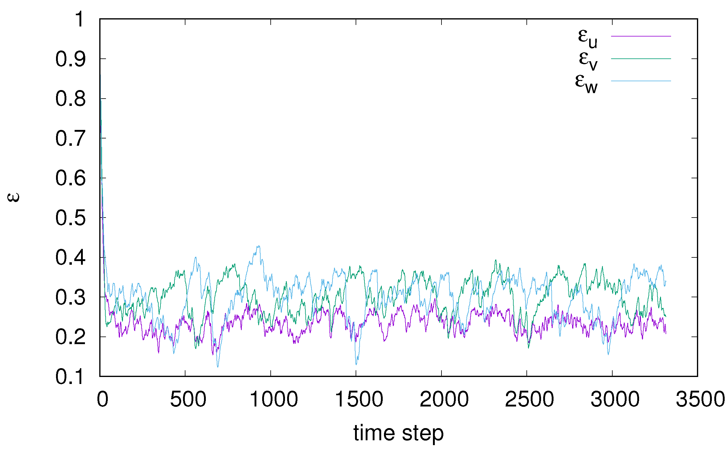
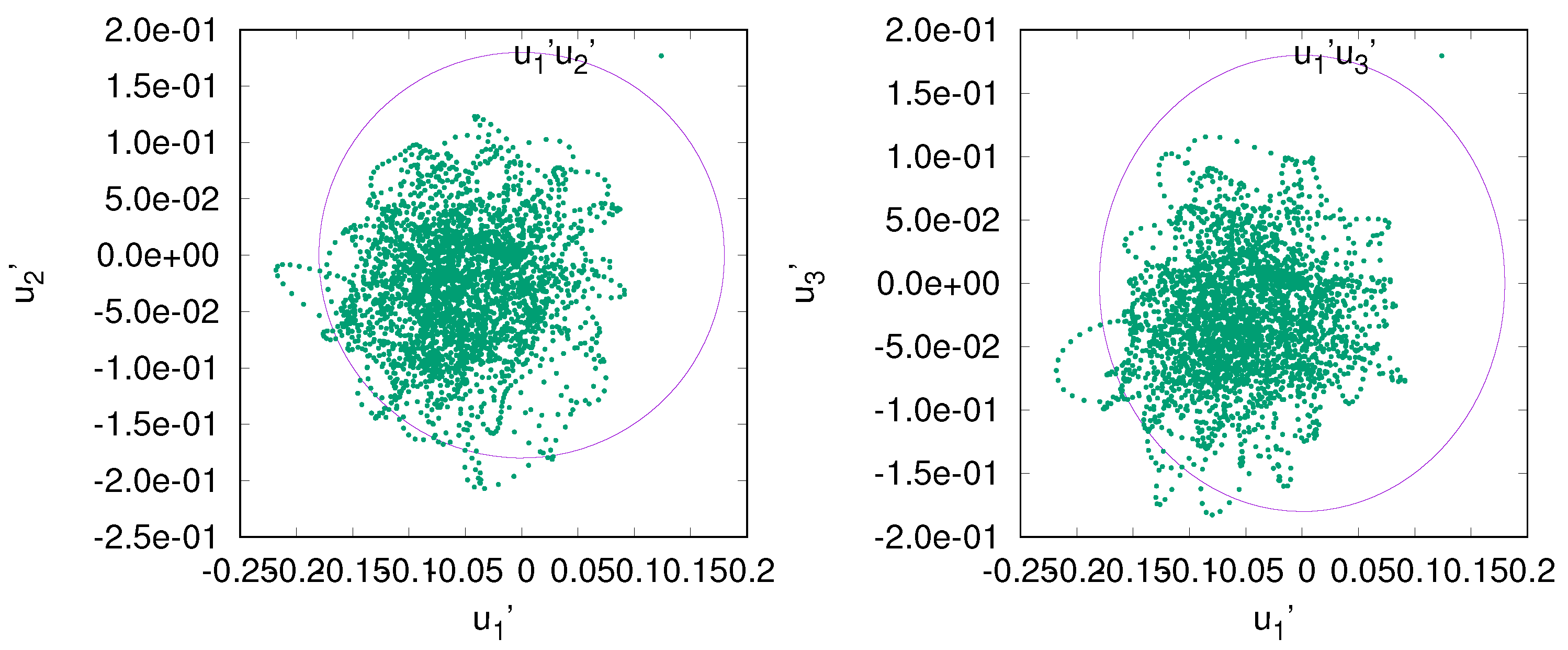
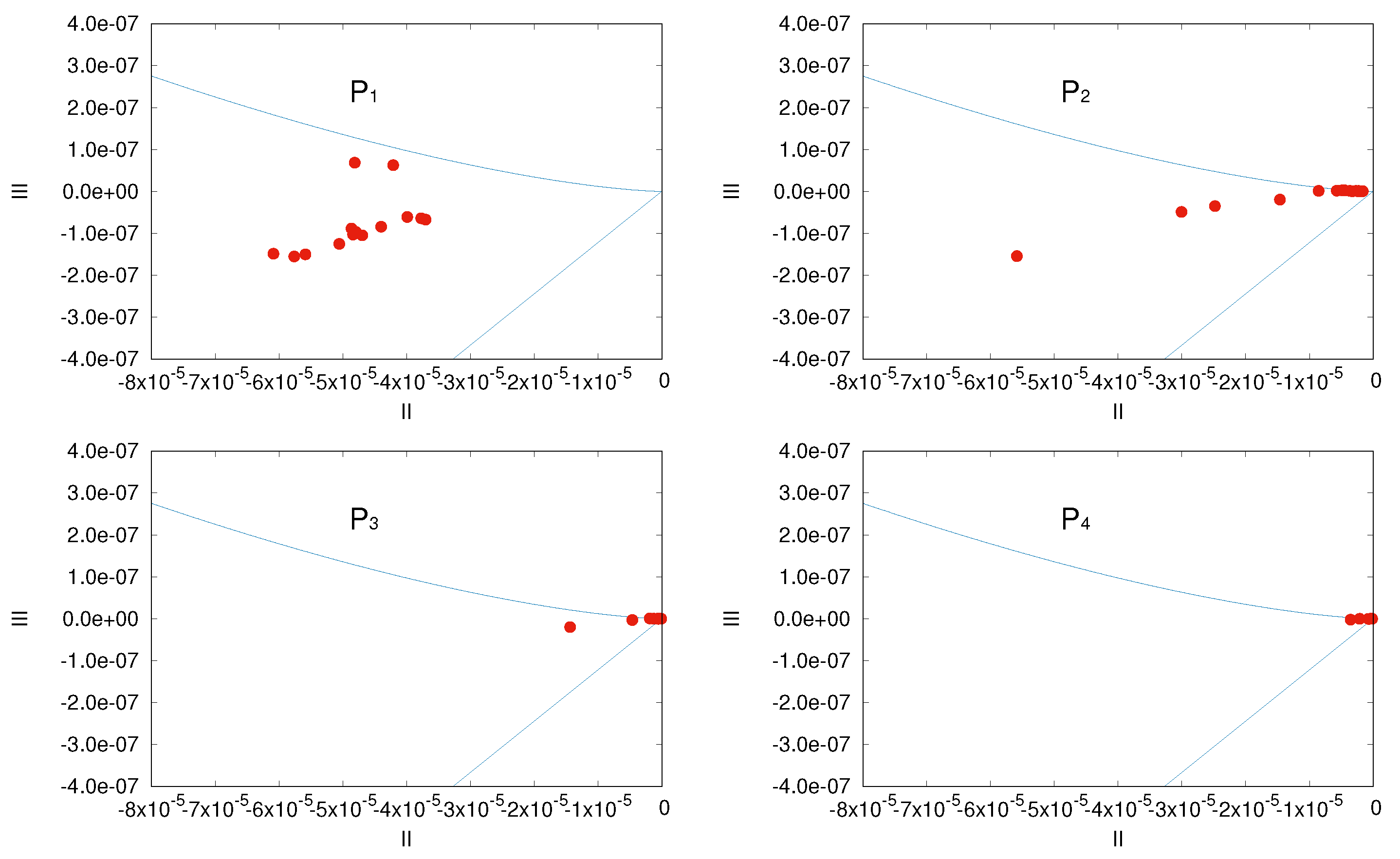
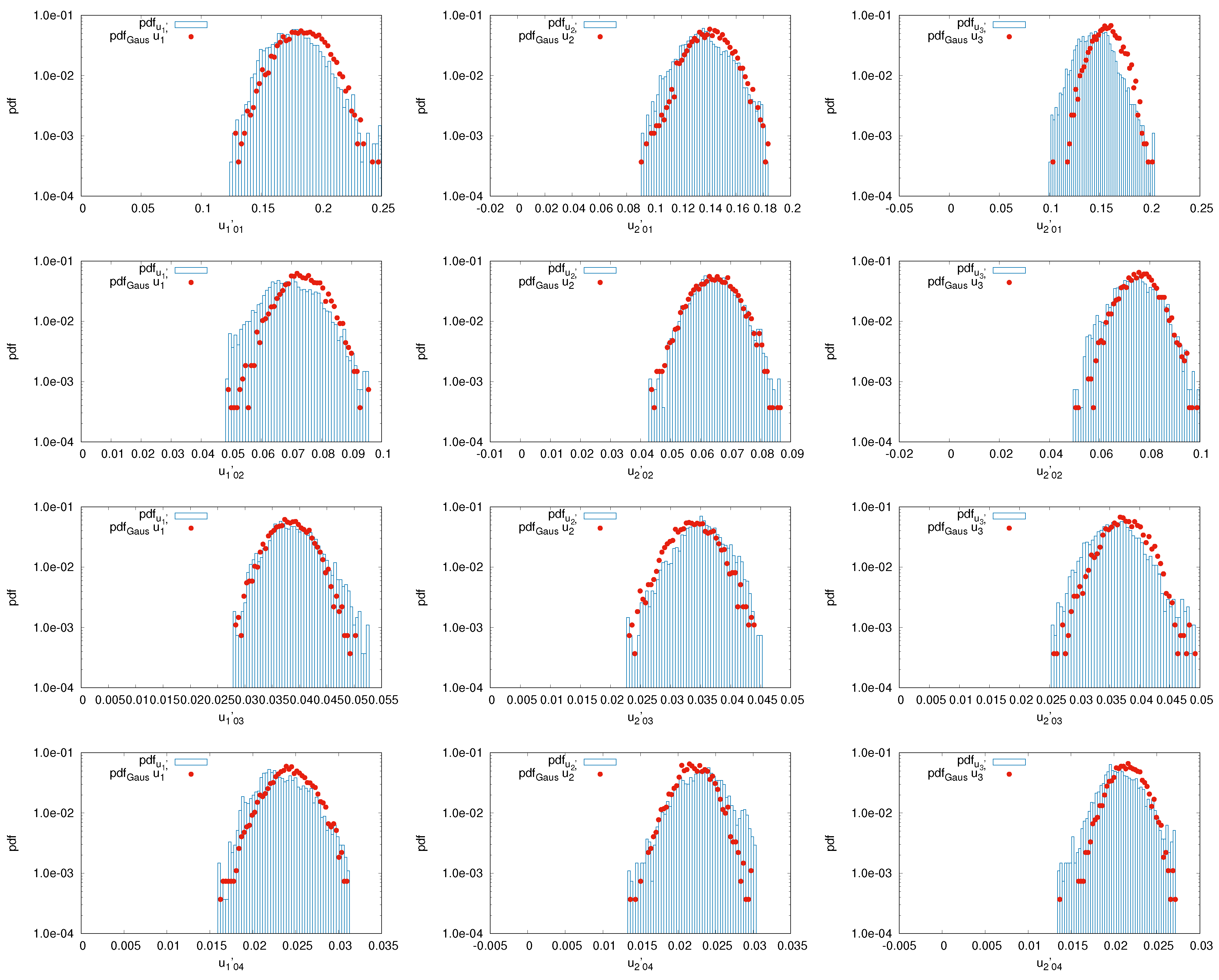
3.1. Turbulent Flow Metrics

For applications to engineering problems, it is fundamental to ensure that the volume force distribution defined in Equation (7) is able to generate a flow field perturbation whose statistical properties are representative of prescribed flow conditions. This is the case of the analysis of hydrokinetic turbine performance in a given deployment site. The high-fidelity modelling of turbine operation implies that the turbulent intensity and other characteristics of the onset flow in the site are adequately accounted for in the simulations. The extraordinary complexity of turbulent flows can be partially characterized through the definition of a dedicated metrics. A discussion on this aspect can be found e.g., in [33]. A primary characterization of a turbulent flow is achieved by analyzing the correlation between fluctuating velocity components. Considering different points at a given time, the spatial correlation tensor is defined as

$$R_{ij}\left(\mathbf{r}\right)=E\left[u_i^{\prime }\left(\mathbf{x}\right)u_j^{\prime }(\mathbf{x}+\mathbf{r})\right]$$

(11)

where the symbol $E\left[\right]$ denotes the expected value operator as shown in Appendix A, and $\mathbf{r}$ is an arbitrary position vector with origin in $\mathbf{x}$. Similarly, the temporal correlation tensor at a given point reads $R_{ij}\left(\tau \right)=E\left[u_i^{\prime }\left(t\right)u_j^{\prime }(t+\tau )\right]$, where $\tau$ is and arbitrary positive or negative time delay from time t. For $\mathbf{r}=0$ or $\tau =0$, the quantity $R_{ij}\left(0\right)$ equals the Reynolds stress tensor.

By introducing the variance of the turbulent flow in the i-th direction as ${\sigma }_i^2=E\left[u_i^{\prime }{u}_i^{\prime }\right]$, simple manipulations show that a direct relationship exists between the trace of tensor $R_{ij}\left(0\right)$ and the variance

$$\mathrm{Tr}\left(R_{ij}\left(0\right)\right)=R_{11}\left(0\right)+R_{22}\left(0\right)+R_{33}\left(0\right)=\sum _{i=1}^3{\sigma }_i^2$$

(12)

where the symbol $\mathrm{Tr}\left(\right)$ denotes the trace operator.

A definition of the turbulent intensity $I_{\infty }$ is then given as

$$I_{\infty }=\frac{1}{u_{\infty }}\sqrt{\sum _{i=1}^3{\sigma }_i^2}$$

(13)

In particular, under homogeneous isotropic turbulence assumptions, one has ${\sigma }_1^2={\sigma }_2^2={\sigma }_3^2$. Recalling Equation (13), turbulence intensity and variance ${\sigma }^2={\sigma }_i^2(i=1,2,3)$ are mutually dependent parameters

$$I_{\infty }=\frac{1}{u_{\infty }}\sqrt{3{\sigma }^2}.$$

(14)

3.2. Generated Turbulence Control Strategy

A key feature of the proposed methodology is that the volume force distribution in Equation (7) can be dynamically modified in order to ensure that the generated turbulent flow matches imposed conditions of the turbulence intensity. This is obtained by combining the numerical solution of Equation (4) with a control algorithm that updates the intensity of the volume force term $\mathbf{f}$ to enforce the realization of target flow properties. To this purpose, a simple control strategy based on a standard Proportional-Integral-Derivative (PID) controller is applied here.

Recalling the direct relationship between turbulence intensity $I_{\infty }$ and variance associated to the velocity components, ${\sigma }_i^2$ $(i=1,2,3)$ in Equation (13), the latter quantities are observed by the control algorithm. Assuming the objective is a homogeneous and isotropic turbulent flow, the variance is equal in all directions and Equation (14) can be used to determine a unique relationship between the desired turbulence intensity $I_{\infty ,des}$ and the desired variance ${\sigma }_{des}^2$.

For an arbitrary distribution of volume force terms, the flow field solution will determine variance terms ${\sigma }_i^2$ that do not match the desired conditions. The following error functions ${\mathcal{E}}_i$ can be defined, where absolute values of standard deviation are used instead of variance

$${\mathcal{E}}_i=\left(|{\sigma }_{des}|-|{\sigma }_i|\right)/\left|{\sigma }_{des}\right|(i=1,2,3).$$

(15)

Quantities ${\sigma }_{des},{\sigma }_i$ are evaluated over a suitable portion of the fluid domain downstream of the turbulence generation region.

The minimization of the error functions above is obtained by the PID control with parameters $k_i,(i=1,2,3)$ defined as follows

$$k_i\left(t\right)=a_{1i}{\mathcal{E}}_i\left(t\right)+a_{2i}{\int }_{t_0}^t{\mathcal{E}}_i\left(t\right)dt+a_{3i}{\partial }_t{\mathcal{E}}_i\left(t\right)(i=1,2,3)$$

(16)

where $t_0<t$, and the coefficients $a_{1i},a_{2i},a_{3i}$ define, respectively, the proportional, integral and derivative control parameters for the i-th velocity component.

Quantities $k_i\left(t\right)$ are used to force variations of the intensity of volume force terms by a simple proportionality relation. The expression in Equation (7) is recast as

$$f_i^{RH}\left(\mathbf{x},t\right)=k_i\left(t\right)\mathrm{\Pi }\left(x_1\right)f_i^{RH}\left(x_2,x_3,t\right)(i=1,2,3)$$

(17)

The PID control interacts with the numerical solution of the Navier–Stokes equations through an iterative procedure as sketched in the flow chart in Figure 4.

4. Computational Model

In the present study, the numerical solution of an incompressible viscous flow is obtained by the Navier–Stokes solver $\chi$–Navis, in-house developed at CNR-INM and extensively validated for a wide range of applications on hydrodynamics studies of marine vehicles and offshore structures.

The numerical solution of Equation (4) is obtained by a Detached Eddy Simulation (DES) approach. A convection–diffusion equation is solved with production and destruction terms and a forcing function that depends on the distance from solid walls. At large distance from a solid boundary, the equation reduces to a Large Eddy Simulation (LES) closure model, see [14] for details.

The dual time stepping approach that generalizes the pseudo-compressibility method proposed in [34] to unsteady problems, is used to solve the fully coupled Navier–Stokes equations. Specifically, the numerical solution of Equation (4) is computed as the asymptotic solution of an auxiliary unsteady problem with additional terms written as pseudo-time derivatives to simulate artificial compressibility. At each step of the physical time, a pseudo-time loop is evaluated to ensure consistent divergence-free velocity and pressure fields.

All spatial operators are approximated by a finite volume technique with pressure and velocity co-located at cell centers. For the viscous terms a standard second order centered scheme is adopted, whereas for the inviscid part a fourth order centered scheme is used. The formal spatial accuracy of this method is second-order (owing to the treatment of the viscous terms). Nevertheless, the use of a less dissipative scheme for the convective terms allows to follow the formation and convection of strong gradients for a considerably longer distance than with the use of a second order-scheme. The convergence ratio for the inner iteration is accelerated by means of local time stepping, an implicit Euler scheme with approximate factorization and a multi-grid technique. The computational domain is discretized by a structured multi-block mesh. Overlapping among grid blocks is made possible by a Chimera technique [35]. More details on the numerical model can be found in [36].

5. Numerical Application

The capability of the proposed methodology to generate turbulent eddies with imposed metrics in an arbitrary onset viscous flow is analyzed here through a simple application. The proposed case study deals with the generation of homogeneous isotropic turbulence with given intensity $I_{\infty }$ into a uniform unbounded flow with constant velocity $u_{\infty }$, hereafter referred to as the nominal flow speed.First, the computational set-up is described. Next, the results of the flow field simulation are presented and discussed.

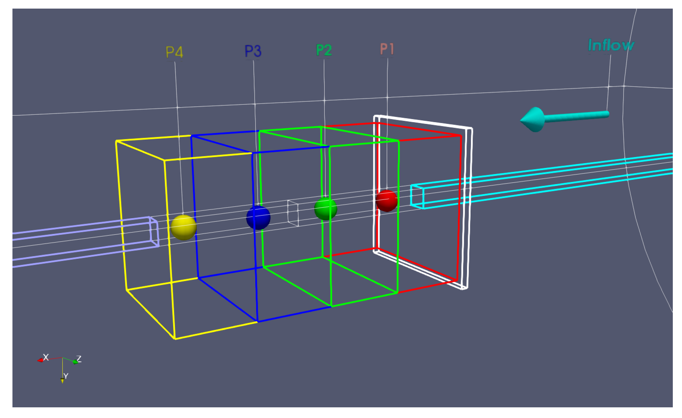
5.1. Computational Set-Up

The computational domain is a cylinder with the two bases representing the inlet and outlet sections, with the cylinder axis aligned with the direction of the unperturbed flow (streamwise direction). Denoting by L a reference length, the cylinder has length $26L$ and radius $9L$. These dimensions are compatible with the set-up for the simulation of the flow field around an isolated horizontal-axis turbine with diameter $D=L$.

A parallelepipedal grid block defines the volume where turbulence is generated (generation block). This block is centred at distance $d_g=14L$ from the inlet section, and is $0.05L$ long in the streamwise direction and $1.4L\times 1.4L$ wide in the normal directions. Downstream of it, another parallelepipedal grid block defines the flow region where the generated turbulence is monitored and statistical properties are evaluated (control block). This block is $2.0L$ long in the streamwise direction and $1.3L\times 1.3L$ wide in the normal directions. These two blocks are immersed into a background grid formed by a toroidal block extended to the external boundary of the computational domain (background block) and internally limited by a thin cylindrical gap that is filled with two partially overlapping parallelepipedal blocks extended from the centre of the domain to the inlet and to the outlet sections (filling blocks).Dimensions and number of cells of each block are given in

Table 1. Computational grid: main blocks size $L_i$ in the i-wise direction ($i=1,2,3$), and number of cells on the finest level.

Block	${\mathit{L}}_1/\mathit{L}$	${\mathit{L}}_2/\mathit{L}$	${\mathit{L}}_3/\mathit{L}$	Cells
Generation	0.05	1.4	1.4	$48\times 128\times 128$
Control	2.0	1.3	1.3	$700\times 128\times 128$
Background	26.0	9.0 (radius)	–	$360\times 60\times 90$

. The discretization refers to the finest grid level, whereas the multi-grid algorithm uses refinement levels, with the coarser grid obtained by removing every second point from the finer grid. In the present study, preliminary results with only two grid refinement levels are presented. A total of five blocks and approximately $2\times {10}^6$ cells on the finest grid level is obtained.

Grid node stretching is applied in background and filling blocks with cells clustering in the flow region downstream of the turbulence generation area, while no stretch is applied on both generation and control blocks to avoid local grid refinement effects on the calculated turbulence metrics. Figure 5 presents views of the overall computational domain and details of the generation and control blocks. It can be noted that the generation block is relatively thin in the streamwise direction, whereas the control block covers a large portion of the flow field.

A velocity condition $\mathbf{u}=u_{\infty }{\mathbf{e}}_1$ is imposed at the inlet section. A gradient pressure condition is imposed at the outlet section and velocity condition is enforced at the external boundary.

The numerical solution is performed by distributed and shared memory parallelization, by using the OpenMP and MPI API. In order to balance the load on all nodes, the control block is split in the streamwise direction into four sub-blocks with an equal number of cells, see Figure 5. Using MPI, the solution on each split block is calculated as a separate process. Once the flow field solution is evaluated, the analysis of statistical properties of the turbulent flow is performed by rebuilding the solution into a single block.

In the present problem, no solid boundaries in the fluid domain exist. In such a condition, the DES model reduces to a LES throughout the computational domain. A time-marching solution for unsteady flows is evaluated. The simulation is initialized with a sudden start. At time $t=0$, the volume force distribution in Equation (17) is initialized with $k_i\left(0\right)={10}^{-5}$. At each time step, the intensity is updated by the PID control strategy in order to achieve imposed values of turbulence in the flow, as described in Section 3.2.

The residuals of velocity components and pressure and the CFL (Courant–Friedrichs–Lewy) number for the solution on the finest grid level are shown in Figure 6. The iteration counter is updated at each step of the pseudo-time loops that are evaluated at each physical time step, see Section 4. In particular, right Figure 6 shows details of 3 full pseudo-time loops between 900 and 1000 cumulative iterations. Velocity components residuals reach values in the order of ${10}^{-4}$ at convergence of the pseudo-time loops, whereas the pressure residual drops to ${10}^{-8}$. Less than 30 steps are necessary to achieve pseudo-time loop convergence. Figure 6 also shows that acceptable values of CFL below 1 are established.

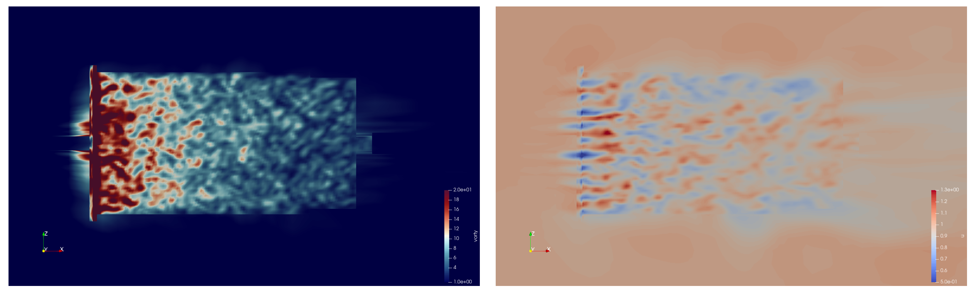
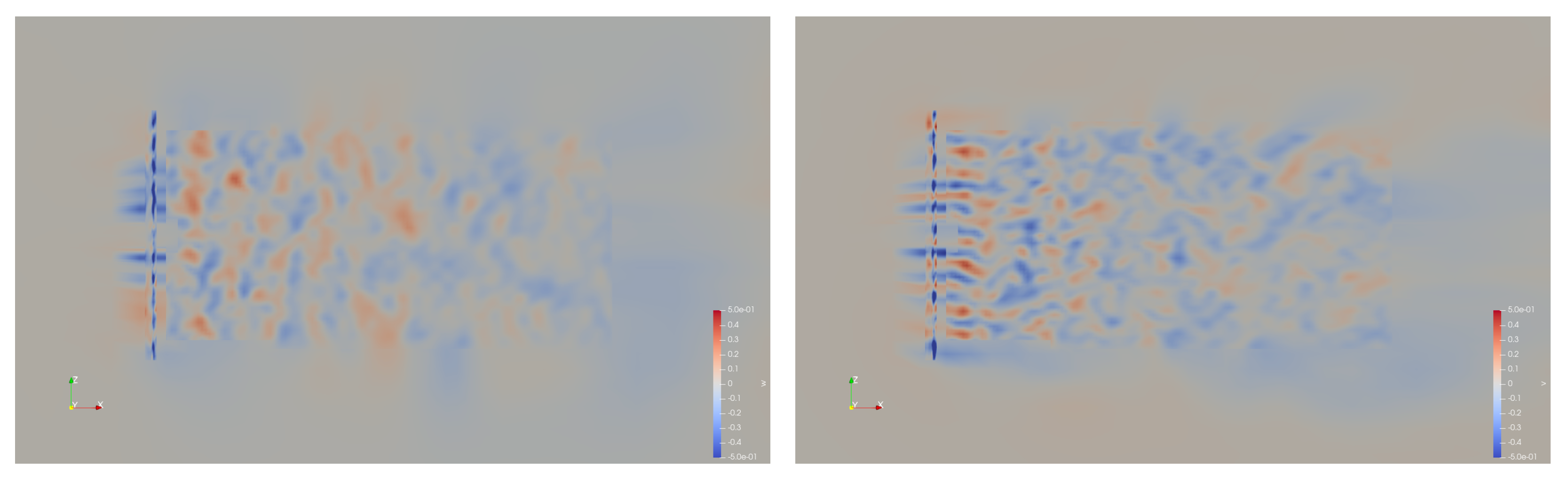
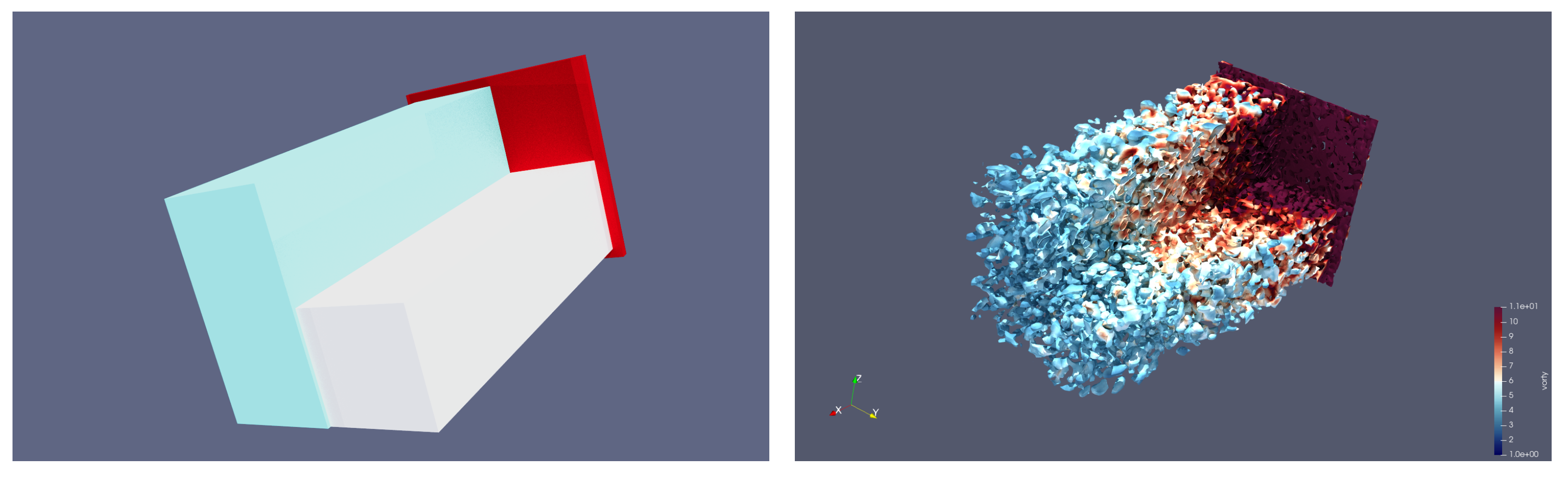
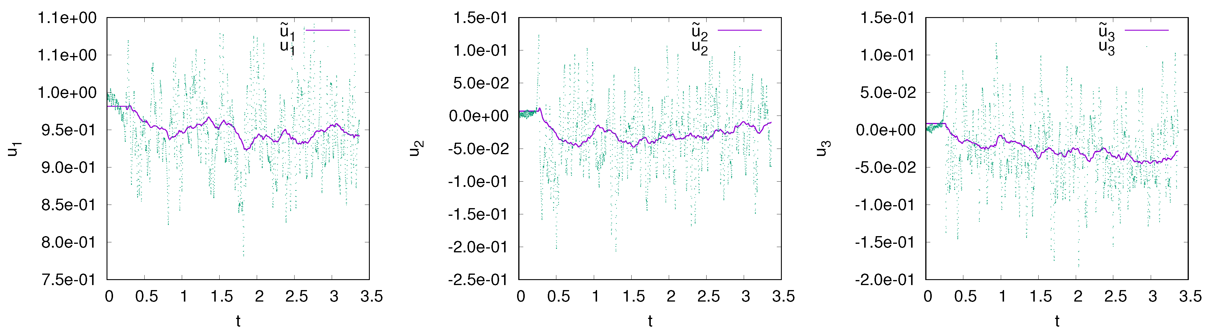
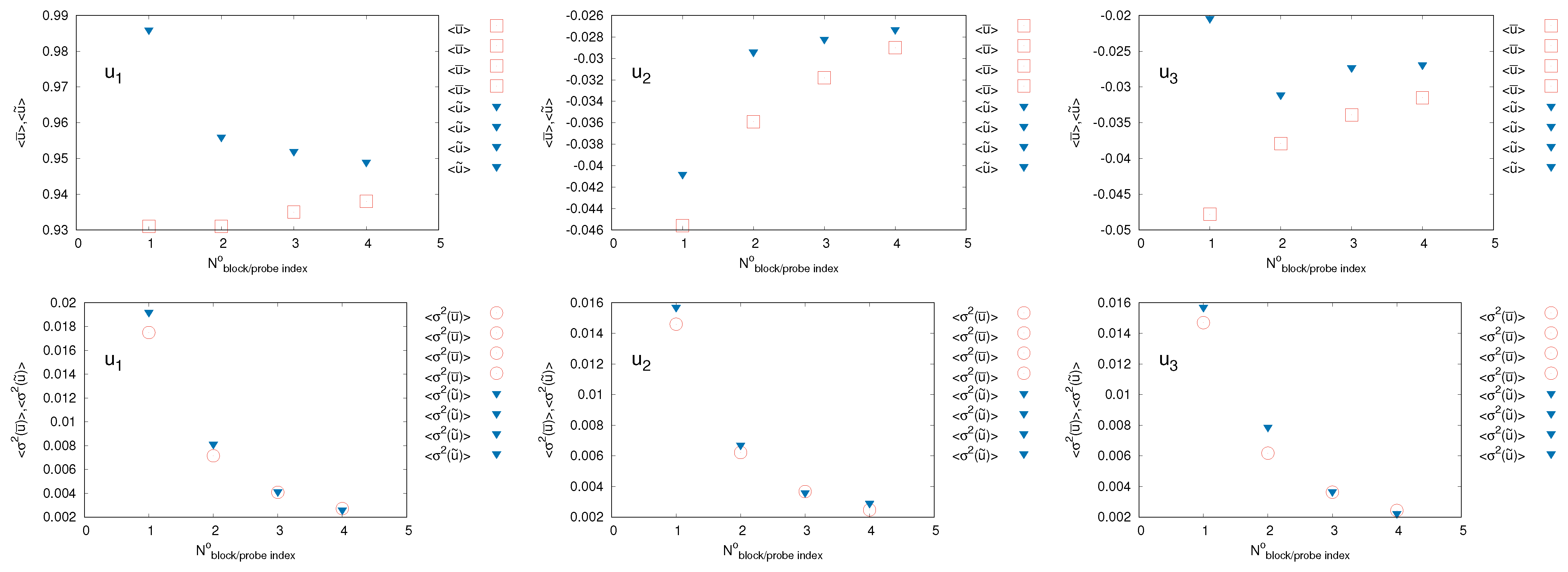
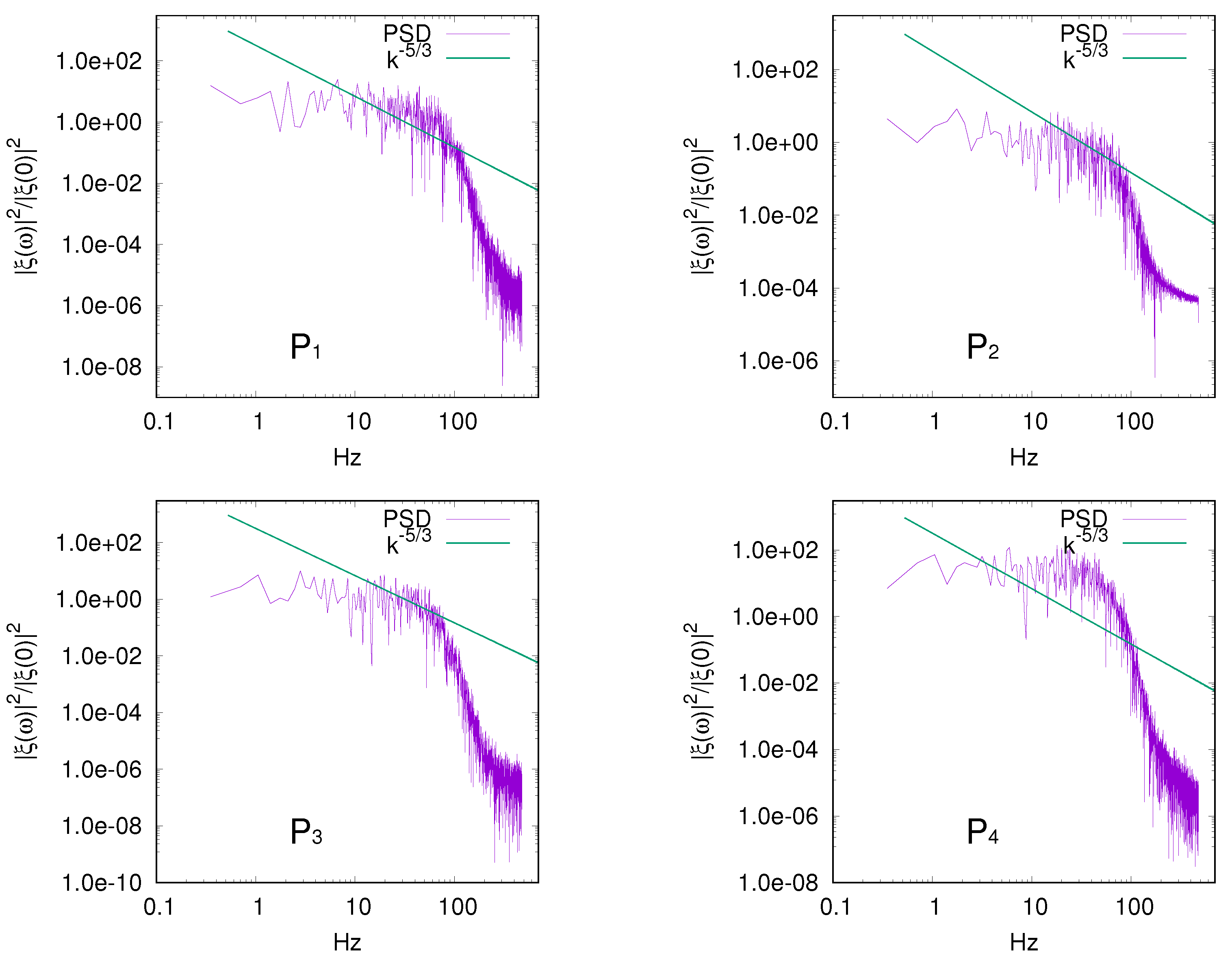
5.2. Flow Field Simulations

The simulation described here deals with a uniform onset flow at $Re=1.25\times {10}^6$. The objective is to generate a homogeneous and isotropic turbulent flow regime with 30% intensity ($I_{\infty ,des}=0.30$) in the fluid region occupied by the grid sub-block 1. Preliminary calculations have shown that this should correspond to an averaged 16% intensity in the whole control block, see Figure 5. The Reynolds number is evaluated as $Re=L{u}_{\infty }/\nu$, where $L=0.5$ m, $u_{\infty }=2.5$ m/s and $\nu =1.004\times {10}^{-6}$ m${}^2/$s. The physical time step used for the time marching solution is $\mathrm{\Delta }t=0.001047$ s. Recalling the grid block dimensions in Table 1, about 780 physical time steps are required to cover at nominal flow speed $u_{\infty }$ the distance between the center of the generation block and the downstream end of the control block. The convection time from the generation block to the downstream end of the control block, $T_{conv}=780\mathrm{\Delta }t$, is taken as a reference to denote the duration of the initial transient-flow phase. In the present calculations, 780 physical time steps correspond to about 10,000 cumulative iterations including physical and pseudo-time steps. Recalling residuals plot in Figure 6, it can be noted that at time $T_{conv}$ the solution has already achieved convergence.

The results presented in this Section describe the flow field solution in the finest grid level. The development of turbulent flow as effect of the interaction between the onset uniform flow and the volume force distribution is illustrated in Figure 7, where the streamwise component of the flow velocity, $u_1$, and of the vorticity magnitude $\zeta =\parallel \nabla \times \mathbf{u}\parallel$ are plotted. Both distributions describe the flow field at a representative time step following the initial transient-flow phase, at $t>T_{conv}$. The onset flow is directed left to right. The perturbation induced by the volume force distribution over a thin region normal to the $x_1$ direction is clearly visible on the left side of the computational domain. The sudden formation of eddies downstream of the generation volume is apparent, whereas outside the wake shed by the volume force region the flow remains unperturbed, except for a transition region where mixing between the turbulent stream and the unperturbed flow is observed. Similarly, snapshots of the velocity components $u_2,u_3$ at the same time step are presented in Figure 8.

A three-dimensional visualization of eddies describing the generated turbulent structures can be obtained by considering the eigenvalues of the tensor ${\mathbf{A}}^2+{\mathrm{\Omega }}^2$, where $\mathbf{A}$ and $\mathrm{\Omega }$ represent, respectively, the symmetric and anti-symmetric parts of the velocity gradient tensor

$$\mathbf{A}=\frac{1}{2}\left(\nabla \mathbf{u}+\nabla {\mathbf{u}}^T\right),\mathrm{\Omega }=\frac{1}{2}\left(\nabla \mathbf{u}-\nabla {\mathbf{u}}^T\right).$$

(18)

By ordering the eigenvalues evaluated at each field point such that ${\lambda }_1\ge {\lambda }_2\ge {\lambda }_3$, vortex structures can be identified by connected regions where ${\lambda }_2$ is lower than a suitable negative value that depends on the flow conditions [35].

Figure 9 presents the ${\lambda }_2$ iso-surfaces at a representative time step, whereas the colormap on the surface denotes the vorticity magnitude $\zeta$. For the sake of clarity, only a portion of the computational domain discretized by generation and control blocks is shown. The inner part of this region is made visible by removing the cells in a quarter of the control block as illustrated in left Figure 9. The ${\lambda }_2$ plot reveals the random fluctuation of the turbulent structures as effect of the mutual interaction among eddies. The diffusion and dissipation of structures as the distance from the generation area increases is witnessed by the vorticity intensity levels associated to the turbulent structures.

The visualization of flow variables such as velocity, vorticity or derived quantities like the ${\lambda }_2$ parameter, provides only a qualitative insight to the generated turbulent flow. Further analysis is necessary to determine key turbulent metrics quantities, and to verify the stationarity of the solution at time $t>T_{conv}$. In particular, the possibility that homogeneous, isotropic turbulence conditions are established with desired turbulence intensity levels is to be investigated.

To this aim, spatial mean values $\overline{u_i}$ and variance ${\sigma }_i^2$ of the velocity components $u_i$ have been evaluated in the flow region occupied by the control block, see right Figure 5.

In particular, denoting by V an arbitrary fluid volume, the spatial mean reads

$${\overline{u}}_i(\mathbf{x},t)=\frac{1}{V}{\int }_V{u}_i(\xi +\mathbf{x},t)d\xi (i=1,2,3)$$

(19)

The quantities are evaluated at each time step and further averaged over time steps $t_k$ such that $t_k>T_{conv}$. The symbol $<>$ is used to denote the arithmetic mean on all samples at time steps $t_k$. The results are presented in

Table 2. Non dimensional averaged mean value $<\overline{u_i}>/u_{\infty }$ and variance $<{\sigma }_i^2(\overline{u_i}/u_{\infty })>$ of the velocity components $u_i(i=1,2,3)$ in the control block and in the 4 sub-blocks.

		$\mathit{i}=1$	$\mathit{i}=2$	$\mathit{i}=3$
Control	$<\overline{u_i}>/u_{\infty }$	0.933	−0.0356	−0.0378
block	$<{\sigma }_i^2(\overline{u_i}/u_{\infty })>$	0.788 $\times {10}^{-2}$	0.686 $\times {10}^{-2}$	0.681 $\times {10}^{-2}$
Sub	$<\overline{u_i}>/u_{\infty }$	0.931	−0.0456	−0.0478
block 1	$<{\sigma }_i^2(\overline{u_i}/u_{\infty })>$	0.174 $\times {10}^{-1}$	0.146 $\times {10}^{-1}$	0.146 $\times {10}^{-1}$
Sub	$<\overline{u_i}>/u_{\infty }$	0.931	−0.0359	−0.0379
block 2	$<{\sigma }_i^2(\overline{u_i}/u_{\infty })>$	0.696 $\times {10}^{-2}$	0.602 $\times {10}^{-2}$	0.599 $\times {10}^{-2}$
Sub	$<\overline{u_i}>/u_{\infty }$	0.935	−0.0318	−0.0339
block 3	$<{\sigma }_i^2(\overline{u_i}/u_{\infty })>$	0.387 $\times {10}^{-2}$	0.347 $\times {10}^{-2}$	0.342 $\times {10}^{-2}$
Sub	$<\overline{u_i}>/u_{\infty }$	0.938	−0.0290	−0.0315
block 4	$<{\sigma }_i^2(\overline{u_i}/u_{\infty })>$	0.250 $\times {10}^{-2}$	0.228 $\times {10}^{-2}$	0.225 $\times {10}^{-2}$

, where averaged mean velocity terms $<\overline{u_i}>$ and variance terms $<{\sigma }_i^2>$ are normalized with respect to the nominal flow speed $u_{\infty }$.

In order to capture the variability of the flow metrics as the distance from the generation region increases, quantities $<\overline{u_i}>$ and $<{\sigma }_i^2>$ evaluated on the whole control block are compared with the corresponding values obtained for each of the four sub-blocks in which the main block is split, as shown in right Figure 5. Specifically, the sub-blocks have identical dimensions and discretization and are numbered 1 to 4 in the streamwise direction. Each block centre is labelled as point $P_i$, with i from 1 to 4, see Figure 10.

From Table 2, a first important result is that the mean velocity in the streamwise direction is lower than the unperturbed flow velocity, with $<\overline{u_i}>/u_{\infty }=0.933$ in the whole control block. The observed 6.67% velocity defect can be explained with the blockage due to the volume force distribution used to generate turbulent eddies. This phenomenon is well known with physical grids that are used in laboratories to stimulate turbulence.

The volume force distribution also determines a deviation of the unperturbed onset flow, with normalized mean values $<\overline{u_2}>/u_{\infty }=-0.0356,<\overline{u_3}>/u_{\infty }=-0.0378$ of the velocity components normal to the nominal streamwise direction $x_1$. Such a flow distortion can be explained with non zero resultants of the randomly generated volume force terms in the $x_2,x_3$ directions.

If mean velocity values from the sub-blocks are considered, it can be noted that the velocity defect in the streamwise direction tends to reduce as the distance from the generation block increases, as effect of diffusion of the wake downstream of the generation block. In particular, $<\overline{u_1}>/u_{\infty }$ increases from 0.931 in sub-block 1 to 0.938 in sub-block 4. Stronger reductions of mean values $<\overline{u_2}>$ and $<\overline{u_3}>$ are observed, with the result that the above mentioned distortion of the flow is partially recovered.

Results in Table 2 for the non-dimensional variance $<{\sigma }_i^2>/u_{\infty }^2$ highlight a significant dissipation of turbulent structures in a narrow region downstream of the generation block. In the nominal streamwise direction, one has $<{\sigma }_1^2/u_{\infty }^2>=0.0174$ in the first sub-block and $<{\sigma }_1^2/u_{\infty }^2>=0.0025$ in the fourth sub-block, whereas the average across the four sub-blocks is 0.0079. In all sub-blocks, the variance in the $x_2,x_3$ directions are almost identical and slightly smaller than the variance in the streamwise direction.

The variance values $<{\sigma }_i^2>$ evaluated on the whole control block, correspond to a turbulence intensity $I_{\infty }=0.1468$ by using the definition in Equation (13). This value is in good agreement with the expected value $0.16$ mentioned at the beginning of this section. However, it is important to recall that the PID control strategy elaborates flow field data from the sub-block 1 to achieve an imposed turbulence intensity. Recalling the dissipative trend observed by comparing results from the four sub-blocks, it can be expected that the turbulence intensity decreases moving from sub-block 1 to 4. Specifically, results for the four sub-blocks and for the whole control block are given in

Table 3. Turbulence intensity by Equation (13) in the control block and in the four sub-blocks.

Control Block	Sub-Block 1	Sub-Block 2	Sub-Block 3	Sub-Block 4
14.68%	21.59%	13.77%	10.37%	8.38%

.

A sound evaluation of the PID control strategy can be made by comparing the turbulence intensity evaluated at the sub-block 1 with the imposed desired value $I_{\infty ,des}=0.30$. From Table 3, a 28% discrepancy between expected and obtained values is found. The role played by the PID controller in the achievement of a given turbulence intensity value is analysed in Figure 11, where the errors ${\mathcal{E}}_i$ evaluated by Equation (15) and referred to the three velocity components, are plotted as a function of the physical time step. The results highlight that the PID errors do not reduce to 0 with the iterations. After few time steps, ${\mathcal{E}}_1$ drops to about 0.25, and 0.35 for the other two components. However, these quantities do not reduce further during the iterative solution and oscillate about the above mentioned values. This trend is consistent with the discrepancy between expected and evaluated turbulence intensity at the sub-block 1 observed above. Results in Table 3 and in Figure 11 highlight that the PID controller used in the present study has a limited capability to enforce a desired amount of turbulence intensity in the flow field.

Once the time-marching solution reaches the fully developed turbulent flow condition, the stationarity of flow properties should be achieved. However, as shown in Figure 11, the PID control used to match an imposed turbulence intensity value introduces some fluctuations in the intensity of the volume force terms that do not extinguish with time. Hence, the capability of the turbulent flow solution to achieve a stationary condition is a key aspect to be investigated. To this purpose, the evolution in time of flow field quantities at selected points is analyzed by considering the points $P_1$ to $P_4$ positioned in the center of each of the four sub-blocks, see Figure 10. The streamwise distances of points $P_1$ to $P_4$ from the center of the generation block are, respectively, $0.275L,0.775L,1.275L,1.775L$. These points are taken as virtual probes in the computational domain and the time series of fluctuating velocity components observed at those locations are processed to determine correlations, Fourier transforms, Power Spectral Density (PSD), and Probability Density Functions (PDF).

First, the flow is analyzed by considering the evolution in time of the time average of velocity components referred to a time bin $T_A$ assumed to be small as compared to the full computational time. For example, by averaging the streamwise velocity component $u_1$, this yields

$${\tilde{u}}_1(\mathbf{x},t)=\frac{1}{T_A}{\int }_{-T_A/2}^{T_A/2}{u}_1(\mathbf{x},t+\tau )d\tau$$

(20)

with arbitrary $t>T_A/2$. The symbol $\widetilde{\left(\right)}$ is used here to distinguish time-bin averaging from standard average evaluated on the full set of time samples $t_k<T_{conv}$, denoted by the symbol $<>$ and used in Table 2 above.

Figure 12 shows the time-bin averages evaluated by Equation (20) for the three velocity components, as the central step t of the time bin increases. In the present analysis, the time-bin interval $T_A$ has been taken equal to 500 time steps.

For comparison, the actual velocity values at each time step are also shown. The results relative to probe no. 4 demonstrate that in spite of the strong random fluctuations of the velocity, and of the oscillations of the volume force intensity induced by the PID controller, the time bin averaged values are almost constant throughout the considered time period.

Non-dimensional mean values and variance evaluated from time series of velocity components at the four probes $P_i$ and $t>T_{conv}$ are presented in

Table 4. Non dimensional mean value $<\widetilde{u_i}>/u_{\infty }$ and variance $<{\sigma }^2(\widetilde{u_i}/u_{\infty })>$ of velocity components $u_i(i=1,2,3)$ from time series at probes $P_j$ ($j=$ 1 to 4) and $t>T_{conv}$.

		$\mathit{i}=1$	$\mathit{i}=2$	$\mathit{i}=3$
Probe $P_1$	$<\widetilde{u_i}>/u_{\infty }$	0.986	−0.041	−0.020
	$<{\sigma }^2(\widetilde{u_i}/u_{\infty })>$	0.193 $\times {10}^{-1}$	0.156 $\times {10}^{-1}$	0.156 $\times {10}^{-1}$
Probe $P_2$	$<\widetilde{u_i}>/u_{\infty }$	0.956	−0.029	−0.031
	$<{\sigma }^2(\widetilde{u_i}/u_{\infty })>$	0.810 $\times {10}^{-2}$	0.672 $\times {10}^{-2}$	0.792 $\times {10}^{-2}$
Probe $P_3$	$<\widetilde{u_i}>/u_{\infty }$	0.952	−0.028	−0.027
	$<{\sigma }^2(\widetilde{u_i}/u_{\infty })>$	0.410 $\times {10}^{-2}$	0.360 $\times {10}^{-2}$	0.372 $\times {10}^{-2}$
Probe $P_4$	$<\widetilde{u_i}>/u_{\infty }$	0.949	−0.027	−0.027
	$<{\sigma }^2(\widetilde{u_i}/u_{\infty })>$	0.260 $\times {10}^{-2}$	0.292 $\times {10}^{-2}$	0.221 $\times {10}^{-2}$

.

The above results, obtained by time averaging data from a single probe, confirm the key trends observed from spatial averaging on each sub-block in Table 2. A non negligible velocity defect in the streamwise direction, and a significant reduction of variance terms ${\sigma }_i^2$ as the distance from the turbulence generation region increases are found in Table 4. A quantitative comparison among results from the two tables is presented in Figure 13. Specifically, non-dimensional mean velocity terms $\overline{u_i}/u_{\infty }$ are compared in the top line plots. A significant discrepancy is observed between spatial averages on sub-blocks and corresponding quantities from probe signals at each sub-block center. The differences tend to rapidly reduce from sub-block 1 to sub-block 4, that is, moving downstream of the turbulence generation region. Specifically, the discrepancy at probe/sub-block 4 for quantity $\overline{u_1}/u_{\infty }$ is only 1.2%, whereas larger values equal to 7.4% and 16.7% are found, respectively, for the $u_2$ and $u_3$ components whose absolute values are very small.

Considering non-dimensional variance terms ${\sigma }_i^2/u_{\infty }^2$, bottom line plots in Figure 13, the differences between the two data sets are small on the upstream blocks and tend to vanish moving further downstream. These results demonstrate that the generated turbulent flow field tends to spatial homogeneity at some distance downstream of the generation region, and as the solution evolves, stationarity of mean velocity components is also established with a good approximation. Except for a narrow region in proximity of the turbulence generation block, a good agreement between spatial and time averages is found. It may be concluded that the generated turbulent field has an acceptable level of ergodicity.

For the sake of completeness, time series of the standard deviation of each flow velocity component are presented in Figure 14. Specifically, time-bin averaged data from single probes at sub-block centers and spatially averaged data over each sub-block are compared.

Figure 15 presents the time auto-correlation $R_{ii}\left(\tau \right)$ defined in Section 3.1, applied here to the velocity components at probe $P_4$. As expected, the correlation rapidly drops to very small values as the correlation time increases. The integral time scale $\mathbb{T}$ can be evaluated as

$$\mathbb{T}=\frac{1}{R_{ii}\left(0\right)}{\int }_0^{\infty }{R}_{ii}\left(\tau \right)d\tau (i=1,2,3)$$

(21)

Considering as example the probe $P_1$, the following values are obtained: ${\mathbb{T}}_{u_1}=7.06\times {10}^{-3}$, ${\mathbb{T}}_{u_2}=1.3\times {10}^{-3}$, ${\mathbb{T}}_{u_3}=2.98\times {10}^{-3}$.

The Power Spectral Density (PSD) of the kinetic energy is evaluated as

$$S\left(f\right)=\frac{1}{\sqrt{2\pi }}\sum _{n\in \mathbb{Z}}{e}^{-i2\pi fn}R\left(n\right),f\in [0,1]$$

(22)

where $R\left(n\right)=E\left[X_n{X}_0\right]$ is the autocorrelation function of a stationary random process $X_n$ and $n\in \mathbb{Z}$ is an arbitrary integer number. Figure 16 presents the PSD calculated at probes $P_i$. In all cases, a frequency range where data are aligned with the Kolmogorov −5/3 law is present. For probes 1 and 2, this range approximately extends between 10 and 100 Hz, whereas it is narrower for probes 3 and 4.

In order to estimate the anisotropy of the turbulent flow, the analysis of the correlation tensor as proposed in [37], is performed. Figure 17 depicts the position of velocity component pairs $(u_1,u_2)$ (left) and $(u_1,u_3)$ (right) in the corresponding $(u_1,u_2)$ and $(u_1,u_3)$ planes. The results are referred to velocity samples from each cell in the control block. With few exceptions, all pairs fall within a circle centered in the origin. This provides a qualitative estimate of the isotropy of the generated flow field. A relative eccentricity of pairs towards negative $u_2$ and $u_3$ values is observed, as already noted by flow visualizations in Figure 8.

Following [33,38], further information can be obtained from the invariants of the tensor $\mathbf{S}$ defines as $S_{ij}=R_{ij}\left(0\right)-1/3R_{ii}\left(0\right){\delta }_{ij}$.

To this purpose, the first three tensor invariants are considered

$$\mathbb{I}=S_{ii};\mathbb{II}=\frac{1}{2}[{\left(S_{ii}\right)}^2-S_{ii}^2];\mathbb{III}=det\left(\mathbf{S}\right),$$

(23)

In particular, the isotropy of a random signal can be investigated by mapping events in the $(\mathbb{II},\mathbb{III})$ plane. Two lines departing from the origin $(0,0)$ delimit the region where invariant pairs $(\mathbb{II},\mathbb{III})$ for a random signal are expected. A perfectly isotropic signal is characterized by invariant values $\mathbb{II}=0$ and $\mathbb{III}=0$. Figure 18 presents the results for the generated turbulent flow. Specifically, the events corresponding to 20 representative time steps at the four virtual probes $P_i$ are considered in separate diagrams. All events are within the feasible region, and points tend to cluster close to the origin as the distance of the probe from the generation region increases (top to bottom, left to right in the figure).

The results highlight that at some distance downstream from the generation region, the generated turbulent structures evolve into a nearly isotropic flow.

Further insight to the isotropy in the established turbulent flow can be obtained by evaluating the Probability Density Function (PDF) of the velocity components at the four probes $P_i$ and comparing with a normal Gaussian distribution. The results are shown in Figure 19 for the three velocity components and all probes $P_i$, with $i=$ 1 to 4. The probes PDFs are compared with Gaussian distributions with same mean values and variance as the calculated velocity components, as described in Table 2 and Table 4 above. With some approximation, the evaluated PDFs for all combinations of probe and velocity component fairly match the corresponding Gaussian distributions. Some deviations with significant skewness and kurtosis are found in the distributions for cases $u_1\left(P_1\right)$ and $u_1\left(P_2\right)$ (respectively, first and second line from top, left column), $u_2\left(P_1\right)$, $u_2\left(P_3\right)$ and $u_2\left(P_4\right)$ (respectively, first, third and forth line from top, center column), and $u_3\left(P_2\right)$, $u_3\left(P_3\right)$ (respectively, second and third line from top, right column). It can be noted that the deviations from the expected Gaussian distribution do not present a clear trend with the position of the considered probe.

5.3. Discussion

The methodology outlined in Section 3 provides a simple formulation to generate a random perturbation and simulate onset turbulence in the numerical solution by CFD of an arbitrary viscous flow. The perturbation originates by an obstacle to the unperturbed flow that is modelled as a distribution of volume forces. A direct analogy is found with physical grids used in the experimental field to generate turbulent flows in tunnel test sections. The modelling of a physical grid as a volume force distribution is computationally quite efficient as compared with the representation of physical grid elements as solid boundaries in the computational domain. In addition to that, the volume force distribution can be dynamically adjusted to modify the flow field perturbation that is generated. In the present approach, a full variability of the perturbation is obtained by a volume force distribution that is randomly variable in time and space and whose intensity can be further scaled through a dedicated control strategy.

The numerical application illustrated in Section 5 has been performed with the objective to investigate if such a simple and computationally efficient model can generate flow field perturbations that are representative of real turbulent flows. In spite of its extreme simplicity, the proposed numerical application provides an appealing case study. The methodology implies that a grid block is dedicated to the volume force distribution. The turbulent structures generated within this block are shed downstream in a flow region that gradually expands in the direction normal to the streamwise direction as effect of the diffusion of turbulent eddies. A control strategy is applied to dynamically adjust the intensity of volume force terms and establish desired levels of flow turbulence. This implies that relevant statistical flow properties are evaluated at virtual probes and over control volumes in suitable positions in the computational domain. In the present numerical application, a grid block covering a portion of the field downstream of the generation area has been considered to collect data for the control algorithm (sub-block 1 in Figure 5). In general, the use of a dedicated control block is not necessary. Nevertheless, the time stepping of the solution and the spatial discretization of the domain portion used to collect input data for the control strategy should be adequately sized for the correct evaluation of statistical properties as mean, variance and correlation of velocity components, power spectral density, probability density functions. In particular, time stepping and grid refinement are responsible for the length and time scales of the turbulent structures that can be modelled. A simple elaboration of data in Table 1 shows that in the present study, eddies with size larger than approximately 0.02L can be described, assuming that at least a 2 × 2 cells square stencil is necessary to detect a planar eddy.

The results of flow field simulations highlight that the perturbation induced by the volume force distribution is characterized by a rapid evolution downstream of the generation region. The dynamics of the turbulent structures is governed by the model used for the numerical solution of the viscous turbulent flow, as shown in Figure 7, Figure 8 and Figure 9. A DES model has been considered in the present study. At some distance downstream of the turbulence generation area, the flow tends to achieve satisfactory levels of stationarity. Small fluctuations of the velocity components are largely due to time variations of the volume force intensity caused by the PID controller that is not able to reduce to zero the control error (Figure 11). In the downstream region, the flow tends to be ergodic as shown by the good agreement between time averages and spatial averages of the mean velocity and variance, as demonstrated in Figure 13. Similarly, flow anisotropy observed close to the generation region is rapidly reduced moving downstream, Figure 18.

For the particular case considered in the present analysis, it may be concluded that at some distance downstream of the generation region, a fully developed turbulent flow with satisfactory stationarity and isotropy characteristics is established. The quantitative comparison between requested and obtained mean flow velocity and turbulence intensity can be also positively evaluated. As expected, a small velocity defect is observed downstream of the region where volume force terms are imposed, with a 6–7% peak. The unperturbed mean flow velocity is partially recovered as the distance from the generation region increases. The turbulence intensity evaluated in the control volume considered by the PID controller (sub-block 1) underestimates by 28% the desired value. A rapid decay of turbulence intensity is observed in a narrow region downstream of the generation area, whereas uniform values are obtained at larger distance downstream. This result highlights clear limits of the turbulence intensity control strategy implemented in the present version of the model. In particular, the control error is largely affected by the definition of the PID settings, $a_i$ coefficients in Equation (16), and ad-hoc tuning is required to minimize the deviation between calculated and desired turbulence intensity values. The location of the fluid domain volume monitored by the controller is another aspect to be analyzed. In the present study, a control volume close to the turbulence generation region has been used, in order to ensure that a consistent feedback by the controller is provided since the first time steps of the simulation.

The results obtained in the present study provide only an initial verification of the proposed methodology. The capability to generate turbulent flows with different intensity levels and the application to complex configurations with solid bodies immersed into the flow has to be demonstrated. Similarly, the analysis of grid refinement on the properties of the generated turbulent structures is also necessary. This is particularly important to assess the capability of the proposed methodology to generate turbulent flows with physically-consistent power spectral density properties. Present results in Figure 16 reveal deviations of the PSD curves from the expected Kolmogorov −5/3 law that are to be further investigated.

6. Conclusions

A theoretical and computational methodology for the generation of onset turbulent flows with prescribed properties in the numerical simulation of an arbitrary viscous flow has been presented. The proposed technique falls within the class of synthetic volume force methods, in which turbulent eddies are generated by a suitable distribution of volume force terms in the right-hand side of the Navier–Stokes equations. In the present formulation, the distribution is defined as a combination of harmonic functions that are randomly variable in time and space. A control strategy is used to enforce that the generated turbulent structures match an imposed turbulence intensity level and a homogeneous isotropic flow is established. Although the approach is general, the proposed methodology is primarily intended for the computational modelling of hydrokinetic turbines in a turbulent onset flow representative of tidal or riverine installations.

A first numerical application has been presented by considering the injection of homogeneous and isotropic turbulence with 16% intensity into a uniform unbounded flow. Flow field calculations have been performed by Detached Eddy Simulation, by using a computational set-up valid for the analysis of model-scale tidal turbine performance in a real onset turbulent flow. The resulting flow field has been analyzed in terms of flow statistical properties as auto-correlation, power spectral density, probability density functions. The results demonstrate that at small distance downstream of the turbulence generation area, the flow tends to achieve satisfactory levels of stationarity and isotropy. A small velocity defect is observed downstream of the turbulence generation region, whereas the unperturbed mean flow velocity is partially recovered as the distance increases. The mean turbulence intensity evaluated over a control volume underestimates by 28% the requested value, whereas a significant decay of turbulence intensity has been observed at increasing distance downstream of the generation area.

From this notional numerical application it can be concluded that the proposed methodology represents a promising approach to simulate onset turbulent flow conditions. Established flow properties are consistent with the computational analysis of hydrokinetic turbines operating in tidal and riverine sites. Significant improvements of present results are expected by introducing advanced volume force control strategies to replace the simple PID controlled used in these preliminary calculations. The application of the proposed methodology to the computational analysis of single turbines and arrays of turbines is the subject of ongoing work.

References

1. Pecoraro, A.; Felice, F.D.; Felli, M.; Salvatore, F.; Viviani, M. An improved wake description by higher order velocity statistical moments for single screw vessel. Ocean Eng. 2015, 108, 181–190. [Google Scholar] [CrossRef]
2. Gant, S.; Stallard, T. Modelling a Tidal Turbine in Unsteady Flow. In Proceedings of the 18th International Offshore and Polar Engineering Conference (ISOPE’08), Vancouver, BC, Canada, 6–11 July 2008. [Google Scholar]
3. Allmark, M.; Martinez, R.; Ordonez-Sanchez, S.; Lloyd, C.; O’Doherty, T.; Germain, G.; Gaurier, B.; Johnstone, C. A Phenomenological Study of Lab-Scale Tidal Turbine Loading under Combined Irregular Wave and Shear Flow Conditions. J. Mar. Sci. Eng. 2021, 9, 593. [Google Scholar] [CrossRef]
4. Togneri, M.; Pinon, G.; Carlier, C.; Choma Bex, C.; Masters, I. Comparison of synthetic turbulence approaches for blade element momentum theory prediction of tidal turbine performance and loads. Renew. Energy 2020, 145, 408–418. [Google Scholar] [CrossRef]
5. Allmark, M.; Ellis, R.; Ebdon, T.; Lloyd, C.; Ordonez-Sanchez, S.; Martinez, R.; Mason-Jones, A.; Johnstone, C.; O’Doherty, T. A detailed study of tidal turbine power production and dynamic loading under grid generated turbulence and turbine wake operation. Renew. Energy 2021, 169, 1422–1439. [Google Scholar] [CrossRef]
6. Sentchev, A.; Thiébaut, M.; Schmitt, F.G. Impact of turbulence on power production by a free-stream tidal turbine in real sea conditions. Renew. Energy 2020, 147, 1932–1940. [Google Scholar] [CrossRef]
7. Mycek, P.; Gaurier, B.; Germain, G.; Pinon, G.; Rivoalen, E. Experimental study of the turbulence intensity effects on marine current turbines behaviour. Part II: Two interacting turbines. Renew. Energy 2014, 68, 876–8892. [Google Scholar] [CrossRef]
8. Sellar, B.G.; Wakelam, G.; Sutherland, D.R.J.; Ingram, D.M.; Venugopal, V. Characterisation of Tidal Flows at the European Marine Energy Centre in the Absence of Ocean Waves. Energies 2018, 11, 176. [Google Scholar] [CrossRef]
9. Sentchev, A.; Thiébaut, M.; Sylvain, G. Turbulence characterization at tidal-stream energy site in Alderney Race. In Developments in Renewable Energies Offshore; CRC Press: London, UK, 2020; pp. 616–623. [Google Scholar] [CrossRef]
10. Tabor, G.; Baba-Ahmadi, M. Inlet conditions for large eddy simulation: A review. Comput. Fluids 2010, 39, 553–567. [Google Scholar] [CrossRef]
11. Calcagni, D.; Salvatore, F.; Dubbioso, G.A.; Muscari, R. A Generalised Unsteady Hybrid RANSE/BEM Methodology Applied to Propeller-Rudder Flow Simulation. In Proceedings of the VII International Conference on Computational Methods in Marine Engineering (MARINE 2017), Nantes, France, 15–17 May 2017. [Google Scholar]
12. Salvatore, F.; Calcagni, D.; Sarichloo, Z. Development of a Viscous/Inviscid Hydrodynamics Model for Single Turbines and Arrays. In Proceedings of the 12th European Wave and Tidal Energy Conference (EWTEC 2017), Cork, Ireland, 27 August–1 September 2017. [Google Scholar]
13. Gregori, M.; Calcagni, D.; Salvatore, F.; Di Felice, F.; Pereira, F.J.A.; Camussi, R. Hybrid viscous/inviscid modelling of a hydrokinetic turbine performance and wake field. In Developments in Renewable Energies Offshore; CRC Press: London, UK, 2020; pp. 553–562. [Google Scholar] [CrossRef]
14. Muscari, R.; Di Mascio, A.; Verzicco, R. Modeling of vortex dynamics in the wake of a marine propeller. Comput. Fluids 2013, 73, 65–79. [Google Scholar] [CrossRef]
15. Na, Y.; Moin, P. Direct numerical simulation of a separated turbulent boundary layer. J. Fluid Mech. 1998, 374, 379–405. [Google Scholar] [CrossRef]
16. Wu, X.; Squires, K.D.; Lund, T.S. Large Eddy Simulation of a Spatially-Developing Boundary Layer. In Proceedings of the 1995 ACM/IEEE Conference on Supercomputing (Supercomputing ’95), San Diego, CA, USA, 3–8 December 1995; Association for Computing Machinery: New York, NY, USA, 1995. [Google Scholar] [CrossRef]
17. Zhu, W.L.; Yang, Q.S.; Cao, S.Y. Applicability research on the turbulent inflow for building les simulation. Kongqi Donglixue Xuebao Acta Aerodyn. Sin. 2011, 29, 124–128. [Google Scholar]
18. Rogallo, R.S.; Moin, P. Numerical Simulation of Turbulent Flows. Annu. Rev. Fluid Mech. 1984, 16, 99–137. [Google Scholar] [CrossRef]
19. Adler, M.C.; Gonzalez, D.R.; Stack, C.M.; Gaitonde, D.V. Synthetic generation of equilibrium boundary layer turbulence from modeled statistics. Comput. Fluids 2018, 165, 127–143. [Google Scholar] [CrossRef]
20. di Mare, L.; Klein, M.; Jones, W.P.; Janicka, J. Synthetic turbulence inflow conditions for large-eddy simulation. Phys. Fluids 2006, 18, 025107. [Google Scholar] [CrossRef]
21. Kraichnan, R.H. Diffusion by a Random Velocity Field. Phys. Fluids 1970, 13, 22–31. [Google Scholar] [CrossRef]
22. Wu, X. Inflow Turbulence Generation Methods. Annu. Rev. Fluid Mech. 2017, 49, 23–49. [Google Scholar] [CrossRef]
23. Lee, S.; Lele, S.K.; Moin, P. Simulation of spatially evolving turbulence and the applicability of Taylor’s hypothesis in compressible flow. Phys. Fluids A Fluid Dyn. 1992, 4, 1521–1530. [Google Scholar] [CrossRef]
24. Choma Bex, C.; Carlier, C.; Fur, A.; Pinon, G.; Germain, G.; Rivoalen, E. A stochastic method to account for the ambient turbulence in Lagrangian Vortex computations. Appl. Math. Model. 2020, 88, 38–54. [Google Scholar] [CrossRef]
25. Rijpkema, D.; Starke, B.; Bosschers, J. Numerical simulation of propeller-hull interaction and determination of the effective wake field using a hybrid RANS-BEM approach. In Proceedings of the Third International Symposium on Marine Propulsors, Launceston, TAS, Australia, 5–8 May 2013. [Google Scholar]
26. Queutey, P.; Deng, G.B.; Guilmineau, E.; Salvatore, F. A Comparison Between Full RANSE and Coupled RANSE-BEM Approaches in Ship Propulsion Performance Prediction. In Proceedings of the ASME 2013 32nd International Conference on Ocean, Offshore and Arctic Engineering, Nantes, France, 9–14 June 2013; ASME: New York, NY, USA, 2013; Volume 7. [Google Scholar] [CrossRef]
27. de Laage de Meux, B.; Audebert, B.; Manceau, R.; Perrin, R. Anisotropic linear forcing for synthetic turbulence generation in large eddy simulation and hybrid RANS/LES modeling. Phys. Fluids 2015, 27, 035115. [Google Scholar] [CrossRef]
28. Spille, A.; Kaltenbach, H.J. Generation of Turbulent Inflow Data with a Prescribed Shear-Stress Profile. In DNS/LES Progress and Challenges, Proceedings of the Third AFOSR International Conference on DNS/LES, Arlington, TX, USA, 5–9 August 2001; Department of Mathematics, University of Texas at Arlington: Arlington, TX, USA, 2001; pp. 319–326. [Google Scholar]
29. Mullenix, N.J.; Gaitonde, D.V.; Visbal, M.R. Spatially Developing Supersonic Turbulent Boundary Layer with a Body-Force-Based Method. AIAA J. 2013, 51, 1805–1819. [Google Scholar] [CrossRef]
30. Weitemeyer, S.; Reinke, N.; Peinke, J.; Hölling, M. Multi-scale generation of turbulence with fractal grids and an active grid. Fluid Dyn. Res. 2013, 45, 061407. [Google Scholar] [CrossRef]
31. Houtin-Mongrolle, F.; Bricteux, L.; Benard, P.; Lartigue, G.; Moureau, V.; Reveillon, J. Actuator line method applied to grid turbulence generation for large-Eddy simulations. J. Turbul. 2020, 21, 407–433. [Google Scholar] [CrossRef]
32. Tangermann, E.; Klein, M. Controlled Synthetic Freestream Turbulence Intensity Introduced by a Local Volume Force. Fluids 2020, 5, 130. [Google Scholar] [CrossRef]
33. Pope, S.B. Turbulent Flows; Cambridge University Press: Cambridge, UK, 2000. [Google Scholar]
34. Chorin, A. A computational method for solving incompressible viscous flow problems. J. Comput. Phys. 1967, 2, 12–26. [Google Scholar] [CrossRef]
35. Jeong, J.; Hussain, F. On the identification of a vortex. J. Fluid Mech. 1995, 285, 69–94. [Google Scholar] [CrossRef]
36. Di Mascio, A.; Broglia, R.; Muscari, R. On the application of the single-phase level set method to naval hydrodynamic flows. Comput. Fluids 2007, 36, 868–886. [Google Scholar] [CrossRef]
37. Kundu, P.; Cohen, I.; Dowling, D. Fluid Mechanics, 6th ed.; Academic Press: London, UK, 2015. [Google Scholar]
38. Choi, K.S.; Lumley, J.L. The return to isotropy of homogeneous turbulence. J. Fluid Mech. 2001, 436, 59–84. [Google Scholar] [CrossRef]
39. Ross, S.M. Introduction to Probability and Statistics for Engineers and Scientist, 5th ed.; Academic Press: San Diego, CA, USA, 2014. [Google Scholar]
Figure 1. Examples of a passive fractal grid (left, from [30]) and of an active grid (right, from [30]) used in wind tunnel experiments.
Jmse 10 01332 g001
Figure 2. Sample harmonic distribution of volume force terms from Equation (6) ( N k = 1 ).
Jmse 10 01332 g002
Figure 3. Sample harmonic distribution of volume force terms with phase and intensity random noise from Equation (7) ( N k = 1 ).
Jmse 10 01332 g003
Figure 4. Iterative turbulence intensity control procedure.
Jmse 10 01332 g004
Figure 5. Layout of the computational domain grid and details of the generation and control blocks (left). The control block is split into four sub-blocks (right).
Jmse 10 01332 g005
Figure 6. Residuals of velocity components and pressure, CFL condition during iteration on physical time and pseudo-time loops (left). Details of pseudo-time loop iteration (right).
Jmse 10 01332 g006
Figure 7. Effect of turbulence generation on the flow field downstream of the generation region. (Left): vorticity magnitude. (Right): u 1 velocity component. Representative time step t 1 > T c o n v .
Jmse 10 01332 g007
Figure 8. Flow velocity components u 2 (left) and u 3 (right) at representative time step t 1 > T c o n v .
Jmse 10 01332 g008
Figure 9. Iso-surfaces of the λ 2 quantity and colormaps of the vorticity magnitude on the generation block and on a portion of the control block (right). Sketch of the considered control block portion (left).
Jmse 10 01332 g009
Figure 10. Control block split into four sub-blocks in the streamwise direction. Sub-block centers are denoted as points P i with i from 1 to 4.
Jmse 10 01332 g010
Figure 11. PID control error for the three velocity components evaluated by Equation (15) and plotted as a function of time.
Jmse 10 01332 g011
Figure 12. Probe no. 4: time series and time-bin average of the velocity components u 1 (left), u 2 (center), u 3 (right), evaluated by Equation (20).
Jmse 10 01332 g012
Figure 13. Comparison of non dimensional mean velocity u i ¯ / u and variance σ i 2 / u 2 ( i = 1 , 2 , 3 ) for all velocity components by spatial averaging on sub-blocks 1 to 4 (top) and by time averaging at probes P 1 to P 4 (bottom).
Jmse 10 01332 g013
Figure 14. Standard deviation of velocity components from time-bin averaging at sub-block probes and from spatial averaging over sub-blocks. Top: u ¯ ( t ) , < u ˜ > ; bottom: σ 2 ( u ¯ ( t ) ) , < σ 2 ( u ˜ ) > . Left to right: velocity components u 1 , u 2 , u 3 .
Jmse 10 01332 g014
Figure 15. Probe no. 4: time auto-correlation R i i ( τ ) of the velocity components u 1 (left), u 2 (center), u 3 (right).
Jmse 10 01332 g015
Figure 16. Kinetic energy Power Spectral Density (PSD) at probes P i with i = 1 to 4, left to right, top to bottom.
Jmse 10 01332 g016
Figure 17. Correlation maps between velocity component pairs ( u 1 , u 2 ) (left) and ( u 1 , u 3 ) (right).
Jmse 10 01332 g017
Figure 18. Isotropy diagrams by using S i j tensor invariants ( II , III ) from Equation (23). Top to bottom, left to right: Probe 1 to 4.
Jmse 10 01332 g018
Figure 19. Probability Density Function (PDF) of velocity components u 1 (left), u 2 (center), and u 3 (right) compared with normal Gaussian distributions. Top to bottom: probes P i , with i from 1 to 4.
Jmse 10 01332 g019