Open Digital Shoreline Analysis System: ODSAS v1.0

Abstract

In this study, we propose a new baseline and transect method, the open-source digital shoreline analysis system (ODSAS), which is specifically designed to deal with very irregular coastlines. We have compared the ODSAS results with those obtained using the digital shoreline analysis system (DSAS). Like DSAS, our proposed method uses a single baseline parallel to the shoreline and offers the user different smoothing and spacing options to generate the transects. Our method differs from DSAS in the way that the transects’ starting points and orientation are delineated by combining raster and vector objects. ODSAS uses SAGA GIS and R, which are both free open-source software programs. In this paper, we delineate the ODSAS workflow, apply it to ten study sites along the very irregular Galician coastline (NW Iberian Peninsula), and compare it with the one obtained using DSAS. We show how ODSAS produces similar values of coastline changes in terms of the most common indicators at the aggregated level (i.e., using all transects), but the values differ when compared at the transect-by-transect level. We argue herein that explicitly requesting the user to define a minimum resolution is important to reduce the subjectivity of the transect and baseline method.

1. Introduction

Diverse and complex natural processes continually change coasts in ways that are physical, chemical, and biological, at scales that range from microscopic (grains of sand) to global (changes in sea level). The regional and local characteristics of coasts control the differing interactions and relative importance of these natural processes. Human activity adds yet another dimension to coastal change by modifying and disturbing, both directly and indirectly, coastal environments and the natural processes of change. Earth-science research on coastal dynamics can quantify these changes and improve our ability to predict coastal responses to human actions (e.g., [1,2]). This study focuses on the quantification of coastal physical change and in particular in the type of change studies commonly referred to as shoreline change analysis (SCA) [3]. To monitor the coastline, although strictly defined as the intersection between water and land surfaces for practical purposes, the dynamic nature of this boundary and its dependence on the temporal and spatial scale at which it is being considered results in the use of a range of shoreline indicators [4]. For practical purposes, the specific shoreline definition chosen is generally of lesser importance than the ability to quantify how a chosen shoreline indicator relates in a vertical/horizontal sense to the physical land–water boundary [4]. In this work, we will use coastline and shoreline as equivalent terms. Regardless of the shoreline indicator acting as a proxy for the coastline, it is always represented as a vector polyline, which is a series of connected vertices that do not form an enclosed shape.

Many researchers and practitioners interested in SCA often separate the mapping stages (mostly done within a GIS) from the time series and trend analyses, which can be undertaken in a programming environment [3]. A GIS or geographic information system is a conceptualized framework that provides the ability to capture and analyze spatial and geographic data. Shoreline differences are often quantified using the “baseline and transect” method [5,6] where the user defines a baseline in the GIS environment and transect lines are then cast perpendicular to the baseline. Different date-stamped shorelines cross the transects at different locations or crossing points. Different metrics of shoreline change are then obtained at each individual transect.

There are a limited number of GIS-based tools to analyze the coastline changes, the most cited being the digital shoreline analysis system (DSAS) [7], but there are other options, such as SCARPS [8] or BeachTools [9,10], which all require a commercial license for ESRI’s ArcGIS to run them. The “Analyzing Moving Boundaries using R (AMBUR)” package does not require a commercial license as it uses the R programming environment, which is free and open software (FOS) [11]. However, AMBUR has the disadvantage of being complex to install and configure the parameters, and it is necessary to edit the baselines and shorelines on a separate GIS, like QGIS or ArcGIS software. These problems, combined with a lack of user support, mean that AMBUR is not attractive for end-users to adopt as a free and open-source option for shoreline analysis in a GIS environment. Lima et al. [12] proposed the validation of the end-point rate (EPR) tool for QGIS (EPR4Q), a built-in QGIS graphical modeler for calculating the shoreline change, using the end-point rate method, and validated the results against DSAS and AMBUR. The unique difference between EPR4Q, AMBUR and DSAS is in the process of transects creation. Lima et al. [12] revealed via validation results that AMBUR, EPR4Q, and DSAS could not produce suitable transects for indented shorelines, considering the scale used in the study cases (transects with 1.0 m spacing) and the shape (rectilinear) of the baselines, and suggested that it will be interesting to analyze the use of other baselines and transect parameters in the future. All the above-mentioned software tools for SCA use only vector objects to delineate the baseline transects.

In this study, we propose a new “baseline and transect” method and software tool that is specifically designed to deal with very indented coastlines and to explicitly incorporate the spatial resolution of the study when delineating the baseline transects. Like DSAS, our proposed method uses a single baseline and allows the user to choose different smoothing and spacing options to generate the transects. Our method differs from DSAS in the way that the smoothing determines the transect orientation by combining raster and vector objects [13]; we also use free open-source software (FOSS), SAGA [14] and the FOS R [15] programming language. Herein, we will refer to our proposed method as the open digital shoreline analysis system (ODSAS). To illustrate the similarities and differences of the SCA results obtained using DSAS and ODSAS, we have compared the SCA results at ten study sites with very irregular coastlines.

The following sections begin with a general description of the overall methodology and the ten coastal study sites selected along the very irregular Galician coastline (NW Spain) and explain how the historical coastline databases were obtained. We continue by describing the DSAS setup, with a special focus on the baseline definition, transect generation and main coastal change metrics obtained. Then, the proposed ODSAS approach is outlined to illustrate how transects are generated, and the shoreline distances are calculated in SAGA GIS, showing how the main coastal change statistics are calculated in R to produce the same metrics of change as calculated by DSAS. In the results section, we show the aggregated and transect-by-transect comparison obtained using both DSAS and ODSAS. In the discussion, we describe in detail the main reasons that explain the similarities and differences of the results obtained. We conclude by indicating that the SCA metrics obtained using the baseline and transect method are very sensitive to the way in which the user creates the transect; therefore, we suggest that the transparency and accessibility of the software tool used to calculate the changes is key. We provide the codes used in ODSAS via the SAGA GIS portal and a dedicated GitHub repository (https://github.com/alejandro-gomez/CoastCR, accessed on 25 November 2021).

2. Materials and Methods

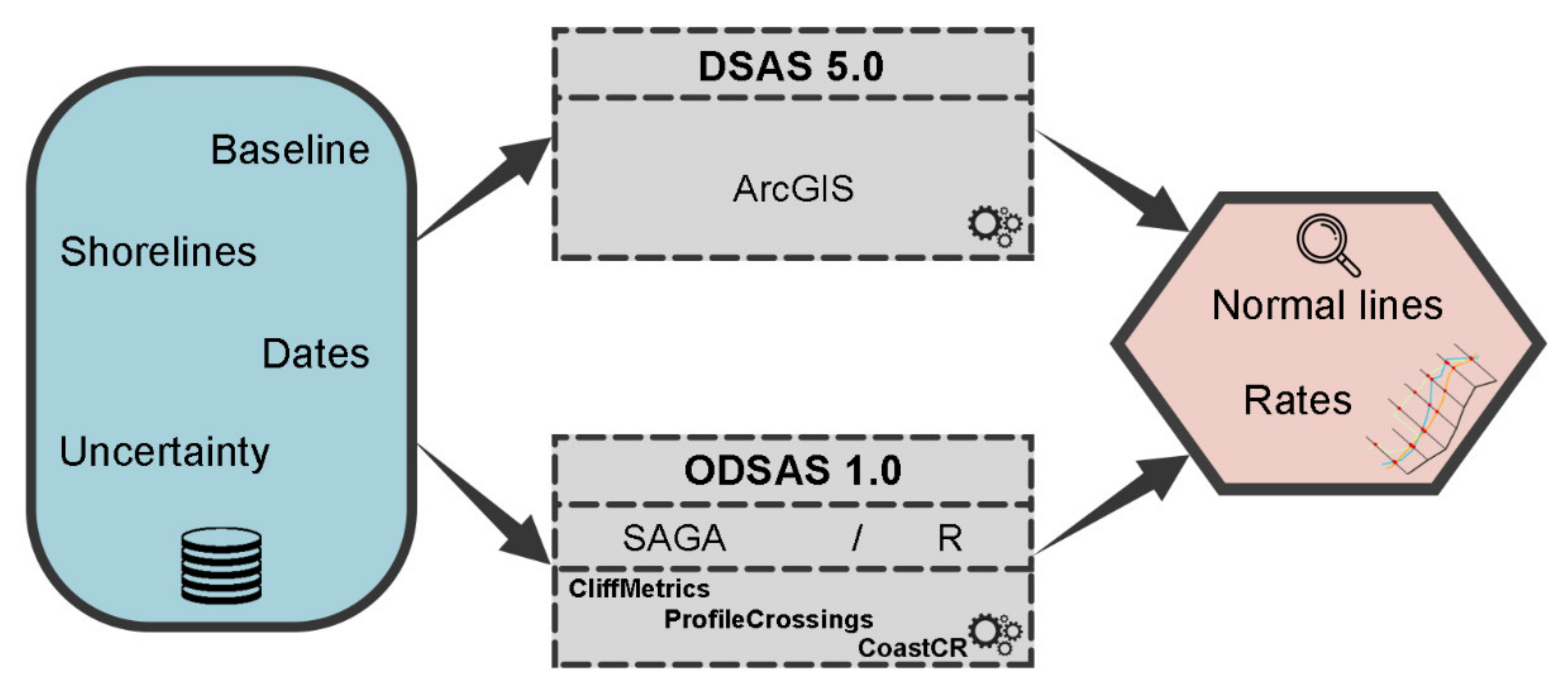
Figure 1 summarizes the methodology followed in this study. We have performed an SCA for ten study sites, with very irregular coastlines, using both the DSAS and ODSAS baseline transect methods and software. We have used different shoreline indicators for the different study sites, including cliff edge line, water–sand edge line and vegetation line. We have used the same baseline for both the DSAS and ODSAS methods, which is parallel to the shoreline and located offshore. For one location, we also tested the sensitivity of SCA results to baseline locations by choosing one baseline located inland and the other baseline located at around the mean sea level horizontal location. Firstly, using the recommended DSAS setup, we obtained the transects and main SCA metrics (described below); then, we iteratively changed the ODSAS setup until we were able to produce similar transects regarding transect orientation, length and location, and produce the same SCA metrics. The results are then compared at both an aggregated level (i.e., metrics for all transects combined) and at a transect-by-transect individual level. For this work, we have used the SAGA v 7.9.1 GIS CliffMetrics tool [13] and have developed two new algorithms: the ProfileCrossings tool for SAGA GIS (https://bgs.sharefile.eu/share/getinfo/s26266f461c343cba, accessed on 25 November 2021) and the CoastCR for R (both new codes, explained herein).

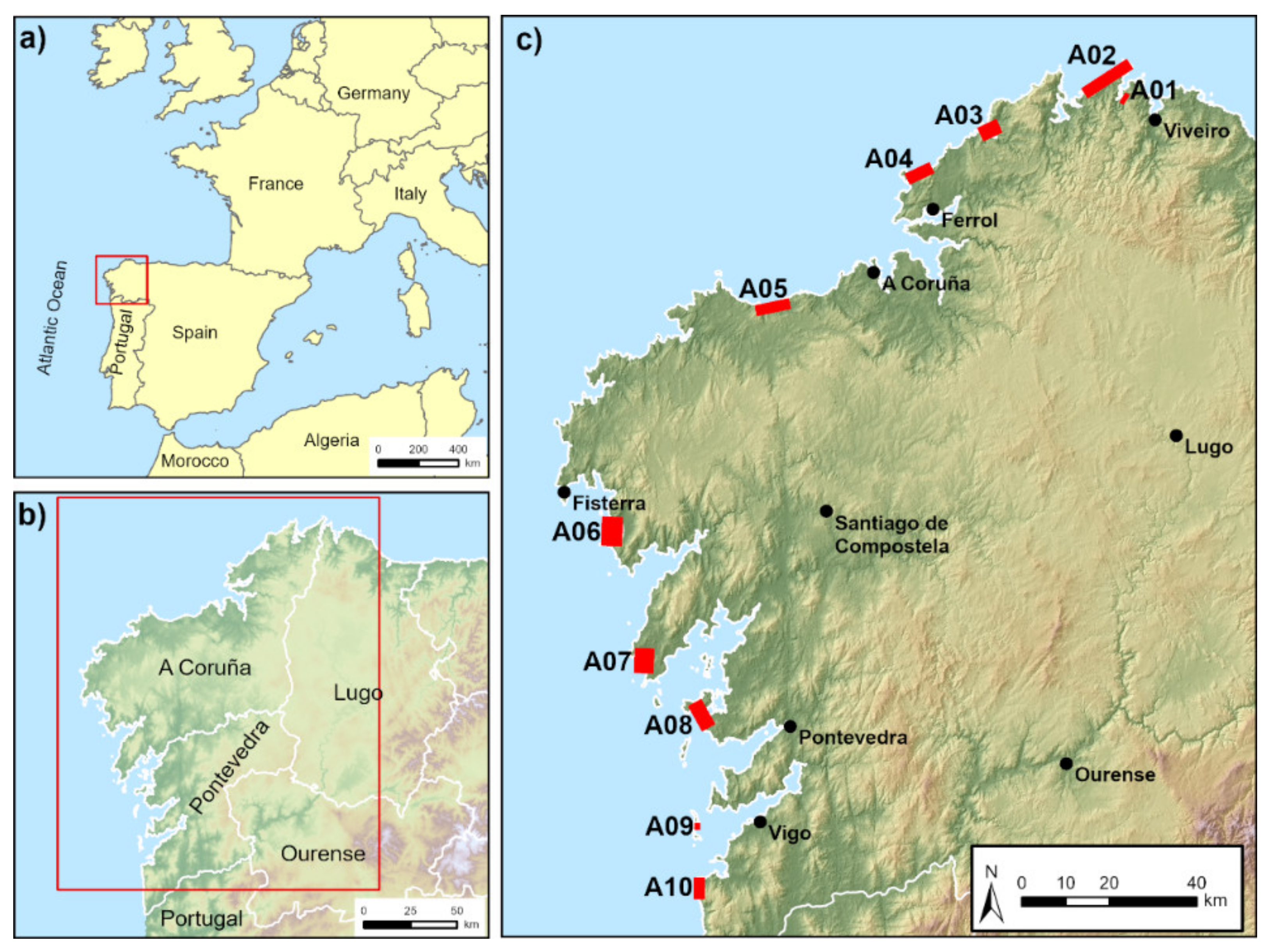
2.1. Study Sites and Historical Coastline Databases

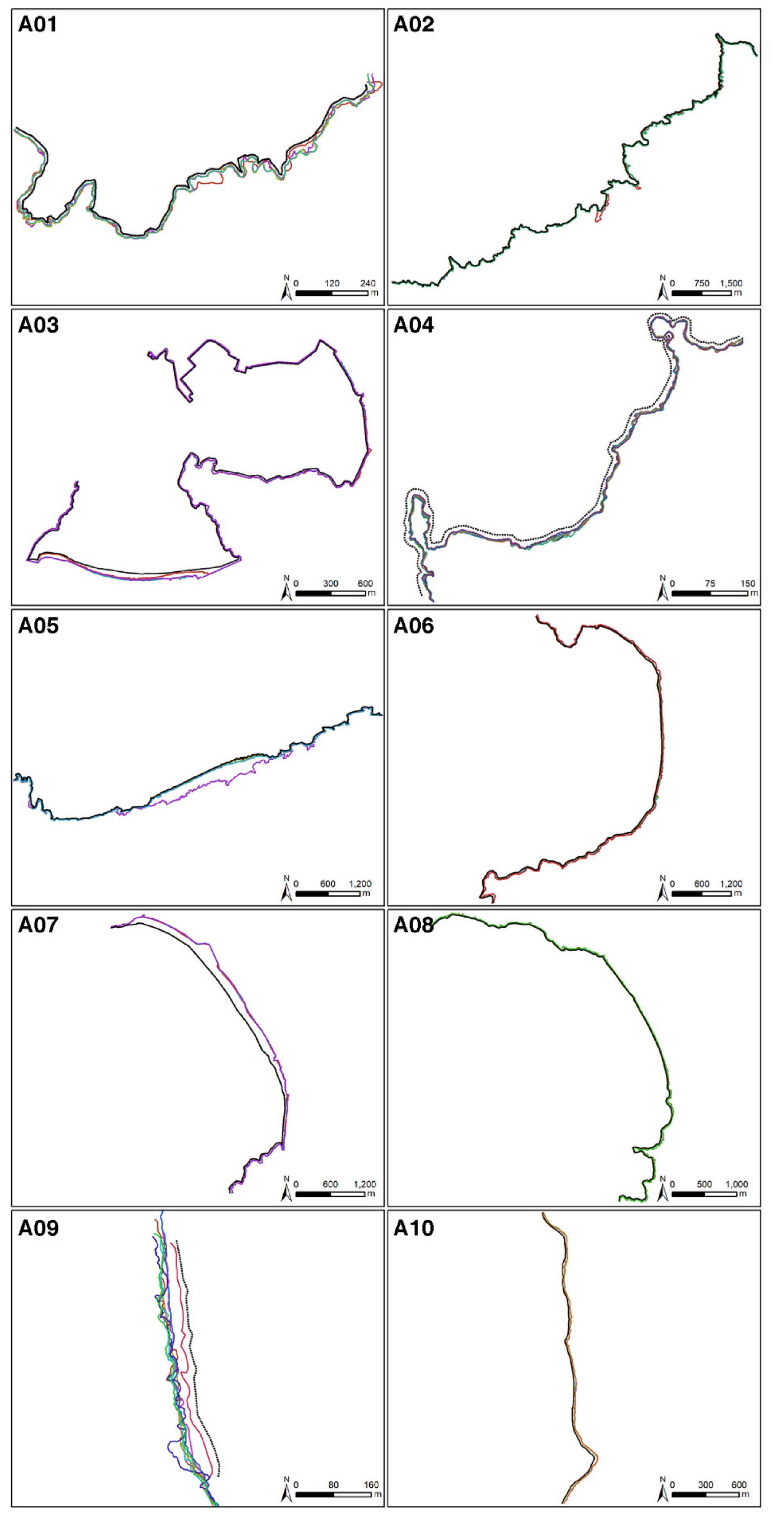
All the study sites used in this project are located along the Galician coast (NW Iberian Peninsula). The ten sites selected (Figure 2) have been studied by the authors in previous projects [16,17], where coastline changes were calculated using DSAS. When combined, these represent very different coastal landform complexes, from small sedimentary sections (coastal plains with sand) to large cliff coastal zones (10- to 20-meter high granitic cliffs, exposed to the main ocean storm waves) and a mix of these classes; the main characteristics of each site are given in

Table 1. Study sites, with their codes, names, and main characteristics.

ID	Name	Length (km)	Description	Analyzed Period *
A01	Espasante	2.7	Low cliffs with rocks at the foot	1956–2017 (4)
A02	Bares	24.2	Different cliff heights and small sedimentary zones	1956–2017 (4)
A03	Vilarube	11.2	Sedimentary sector with low cliffs and a harbor	2010–2017 (3)
A04	Ponzos	1.66	Cliff area with frequent mass movements	2002–2018 (8)
A05	Baldaio	11.9	Sedimentary area with small low cliff zones	1956–2017 (4)
A06	Carnota	13.2	Sedimentary area with low/medium cliffs at the ends	2010–2017 (3)
A07	Corrubedo	8.1	Sedimentary area and low cliffs at the south end	2010–2017 (3)
A08	A Lanzada	10	Sedimentary area in a highly anthropized sector	2010–2017 (3)
A09	Cies Islands	0.8	Sedimentary zone	1956–2017 (8)
A10	Cabo Silleiro	3.2	Rocky coast. Low cliffs and shore platforms	2010–2017 (3)

* The bracketed values show the number of shorelines/dates in each site.

. The Galician coast is the most energetically changeable sector of the Iberian Peninsula [17,18]. This region is a mesotidal coast, with a maximum and mean tidal range of ca. 4 m and 2.5 m, respectively [18]. Marine storms are concentrated in the winter months (November to March) when the wave height, during rare storm episodes, can exceed 10 m (e.g., the Cabo Silleiro buoy in 2014 registered a significant wave height above 12 m in Puertos del Estado [18]).

The NGI (Instituto Geográfico Nacional, Spain [19]) provides free aerial images and orthoimages from all selected sectors during the period 1956–2017 (Table 1). These images have different sources and resolutions, from 1:32,000 in the American flight (1956) to 1:20,000 since 2010. The last orthophotographs have a resolution of 25 cm, facilitating the analysis of smaller features, while the resolution of the older images is considerably poorer, imposing significantly larger uncertainties in terms of feature identification and shoreline delineation. The historical shorelines used in this study were drawn from these aerial image databases, using GIS software and photo-interpretation techniques. In all cases, the mapping scale was 1:500, adapting the contrast and brightness characteristics for better interpretation. The shoreline indicator used as a proxy for the coastline varied between sectors [20]. In cliff areas, the line was drawn using the cliff top as a feature, whereas in the sedimentary zones, the shoreline was drawn using the vegetation edge [4,16,21,22]. The same historical coastline databases were used in both approaches (DSAS and ODSAS). To minimize subjectivity in the comparison, the automatic delineated transect lines produced by both DSAS and ODSAS have not been edited to remove possible outliers.

2.2. Baseline and DSAS Settings

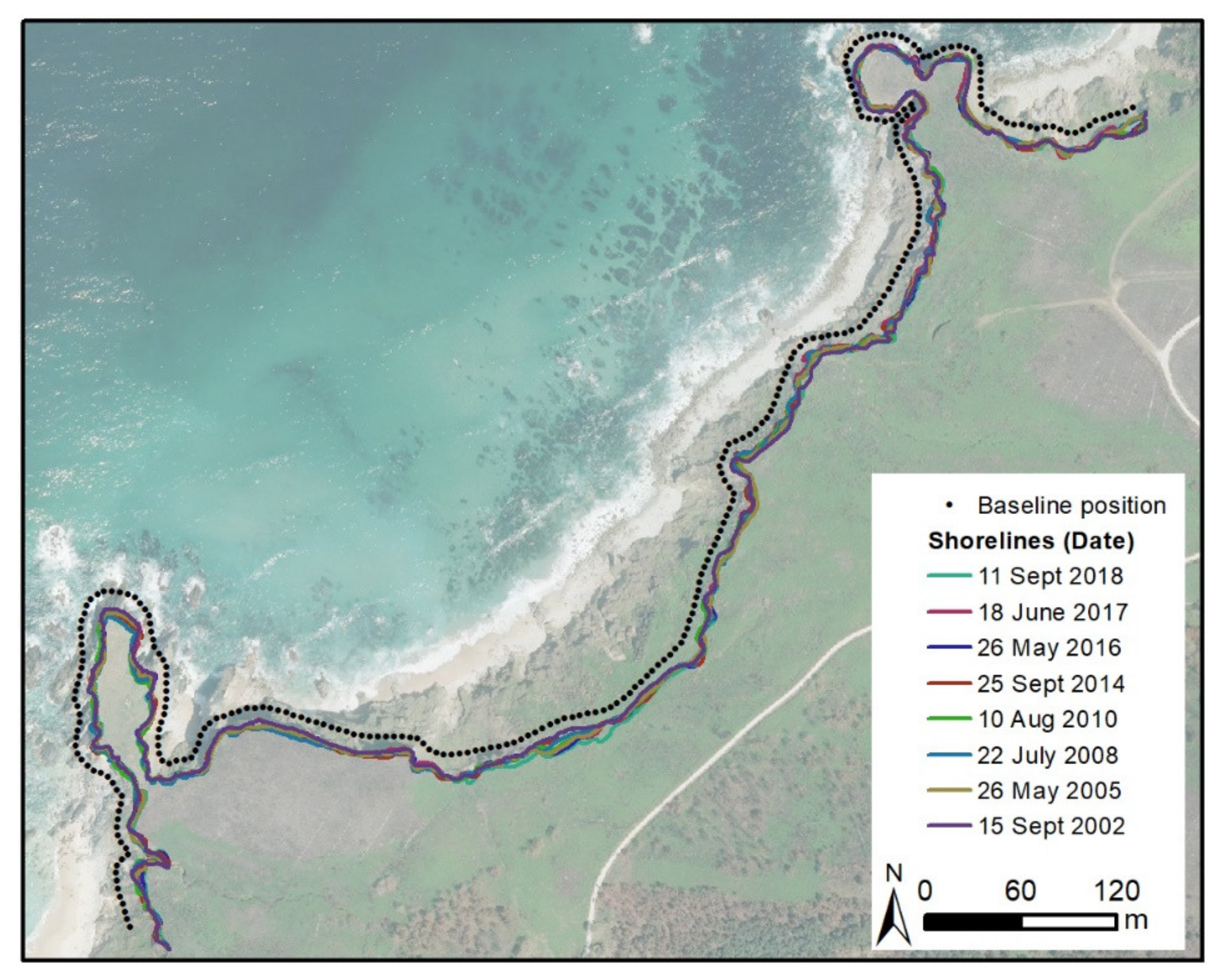
The same baseline has been used for both DSAS and ODSAS approaches. To delineate the baseline for each site, firstly an enveloping polygon was mapped out for all historical coastlines. Then, a continuous line was drawn by hand at the sea edge of the enveloping polygon (offshore) to avoid any sharp edges along the enveloping polygon. Figure 3 shows site A04 as an example, illustrating the resulting baseline (black dots) and its location relative to the historical coastlines for this site. The baseline and historical coastline locations for all study sites are included in Appendix A.

For this study, we have used DSAS software version 5.0 [23] and a setup similar to the one used in previous works conducted by the main author [16,24], briefly described here. The first mandatory DSAS input is a geodatabase that includes all the information necessary to perform the processing. This geodatabase must contain the baseline and historical coastline files. Baseline parameters must be introduced as a vector polyline shapefile, also indicating the relative land position (right or left) and the baseline placement (onshore/offshore/intermediate). For the historical coastlines, the necessary parameters are the date and uncertainty of each line and should select the intersection point between normal lines and shorelines. DSAS allows two possibilities, either landward or seaward, and, in the cases shown here, was always set at seaward [23]. In this project, the baseline position was always offshore, the spacing between transects was 5 m, and the smoothing distance was also 5 m. The remaining DSAS setup parameters are summarized in

Table 2. Main parameters used in setting up DSAS for each study site.

ID	Land Position	Shorelines Uncertainty (m)	Search Distance (m)
A01	Left	1–4	80
A02	Left	1–4	300
A03	Left	1	100
A04	Left	0.5–4	50
A05	Left	1–4	400
A06	Right	1	80
A07	Right	1	300
A08	Right	1	60
A09	Left	1–4	100
A10	Right	1	40

.

2.3. Open Digital Shoreline Analysis System (ODSAS)

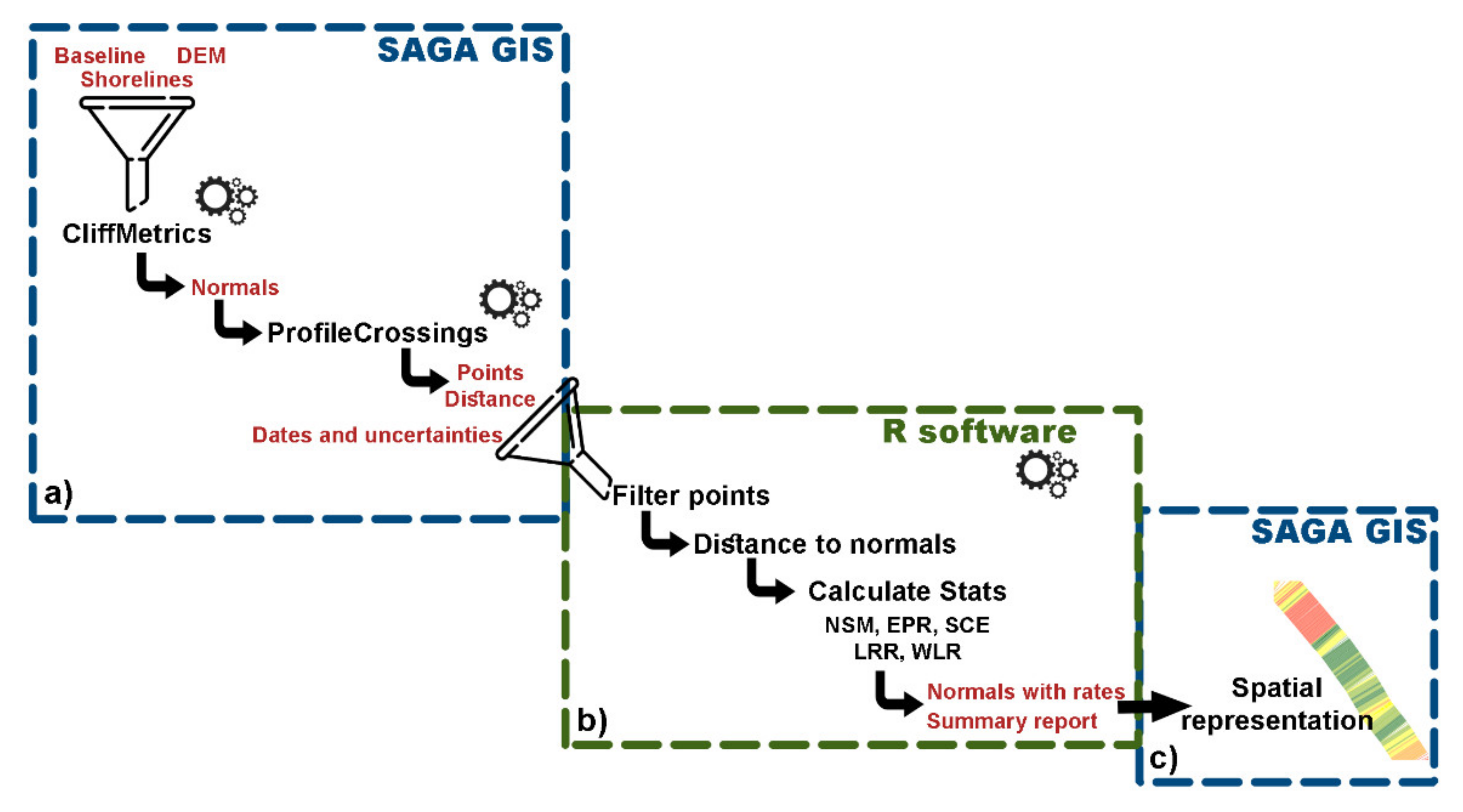
Figure 4 illustrates the new proposed workflow (hereinafter referred to as ODSAS), which uses SAGA GIS, first to obtain transects, intersection points and distances per transects, and secondly, the R environment to obtain the remaining coastline change statistics. The first part uses SAGA-CliffMetrics for transect generation and SAGA-ProfileCrossings to obtain the shoreline distances along each transect. The statistical processes and rates calculation are performed within the R environment, and, as an optional step, the spatial representation and comparison between techniques are conducted in SAGA GIS.

Table 3. Summary of input and output data for the whole ODSAS approach: name, brief description, and type/format.

Name	Description	Type
Inputs
Seaward Side Profile Lines	Normals from baseline to the sea	Line shape
Landward Side Profile Lines	Normals from baseline to the land	Line shape
Coast Lines	Shorelines for each date	Line shape
General Normal Lines	Merge of previous normal lines	Line shape
Coast Lines data	Date and uncertainty for each shoreline	Table (csv)
Outputs
Crossings at Seaward Side	Intersection between normals and coastline at coastal side	Point shape
Crossings at Landward Side	Intersection between normals and coastline at land side	Point shape
Distances to baseline	Merge both crossings with the distances from baseline	Point shape
Normal rates	Normals file with all rates associated with each transect	Line shape
Main statistics	Central tendency statistics for each parameter	Table (png)

summarizes the main inputs and outputs for the proposed ODSAS approach. The unique difference in relation to the DSAS input parameters is in the format required for the baseline; in SAGA-CliffMetrics, the baseline is inputted as a point vector shapefile (i.e., instead of the polyline used in DSAS). To reduce possible influences in the comparison between both methods, the points were generated along the entire baseline at a spacing of 5 m (i.e., the same distance between transects as used in DSAS). The main inputs to run SAGA-ProfileCrossings are the historical coastlines and the transects (at both landward and seaward sides) to the baseline as a vector polyline format. In cases where the baseline is offshore or onshore, the user can employ the same transects in both directions and then remove the false values using the filter method implemented in R (see Section 2.3.2).

SAGA-ProfileCrossings automatically generates an ID for each shoreline, starting at 0 and sorted following the shapefile attribute table. To run R-CoastCR, the input required are: (1) the SAGA-ProfileCrossings output point shapefile, with the distances between the baseline and the intersection points resulting from the transect lines crossing all the historical coastlines; (2) the normal lines shapefile to identify each transept position from SAGA-ProfileCrossings; and (3) an additional table (.csv format), with the historical coastline dates (dd/mm/yyyy) and the uncertainty in meters associated with each one. The order of the coastlines in the shapefile attribute table must be the same as the date/uncertainty table; however, the polylines do not have to appear chronologically.

The baseline transects are generated using SAGA-CliffMetrics (version 1.0) [13] from the same baseline used in DSAS but employed in a points format. This tool generates the transects by a series of vector and raster operations and, therefore, requires a digital elevation model (DEM) as an input file. CliffMetrics generate cross-shore transects perpendicular to a smoothed vector coastline, using a raster-baseline location as the starting point of the transect and a user-defined transect length. The DEM resolution (or grid-cell size) affects the transect starting point location and the user-defined smoothing affects the orientation of the transects. The effects of the DEM resolution on the location of the transect starting points are illustrated in Figure 5, showing the transects obtained using the same baseline but at two different DEM resolutions, fine and coarse, illustrated as grey and black grids, respectively. The transect starting points obtained using the ODSAS method with the fine and coarse grids are shown as green triangles and red squares, respectively. Notice how the distances between these transect starting points and the baseline nodes (blue circles) are smaller for the green triangles than the red squares. The user can then explicitly define the resolution of the study by defining the DEM resolution, which constrains the location of the transect starting point to the nearest raster cell centroid. Notice that the number of transects generated by CliffMetrics will be always equal to or smaller than the number of baseline points. The number will be smaller if the distance between two consecutive baseline points is small enough compared with the DEM resolution, resulting in two different baseline points sharing the same transect starting point. The user, by checking if the number of baseline points is equal to or smaller than the number of transects, now has a numerical indicator of the adequacy of the transect spacing, relative to the resolution of the study.

If, as is the case in this project, we do not need to delineate the baseline from the DEM, the user can simply employ a dummy raster with the desired resolution. For this study, we have generated dummy DEMs for all sites of 1 m of spatial resolution, using the SAGA-Create Grid system. CliffMetrics also requires the following additional parameters: the orientation of the start and end lines (N, E, S, W), the sea position, the length of the normal lines and the smoothing method to generate these lines. The smoothing options are either no smoothing, using the running mean method (this needs a user-defined window size), and the Savitzky–Golay, where it is necessary to have a user-defined window size and the polynomial order. Users need to run CliffMetrics for each side (both land and sea) to generate the landward and seaward transects, respectively. In cases where the user does not have a defined baseline, this could be drawn using CliffMetrics as the line at a given user-defined elevation. CliffMetrics uses a wall-follower algorithm to delineate the coastline along the DEM that best fits the requested elevation.

2.3.1. ProfileCrossings Module

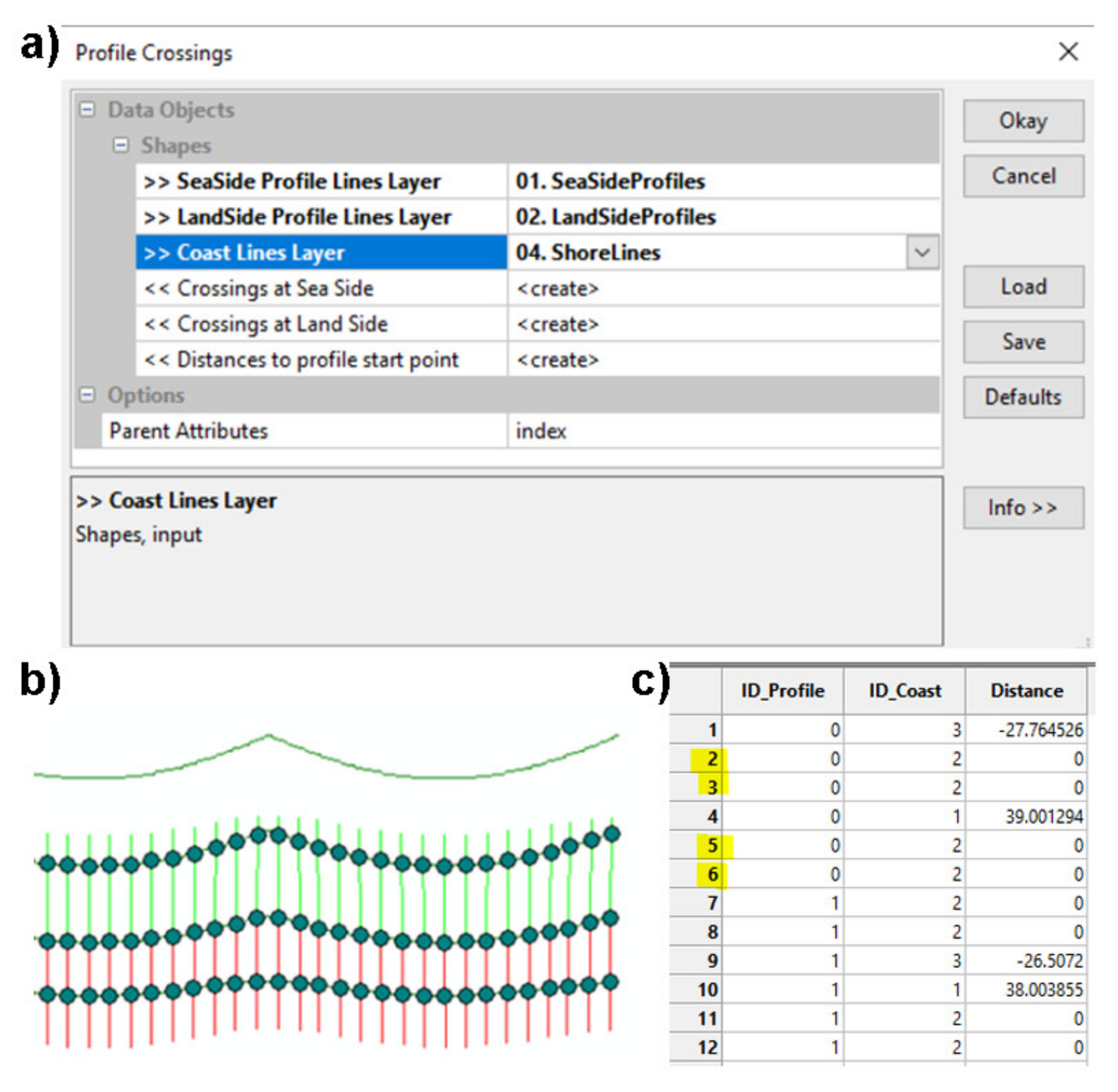
The SAGA-ProfileCrossings tool is a method developed by the authors in collaboration with SAGA developers that measures the distance between each point along a reference baseline to the points where profiles that are normal to the said baseline cross the coastlines to which the user wishes to compare them. The SAGA-ProfileCrossings tool uses normal lines oriented to both sides of the coast, so the user needs to run the CliffMetrics tool twice, changing the sea proximity parameter to obtain two normal files, one oriented to the seaward side and one to the landward side (SeaSideProfiles and LandSideProfiles) (Figure 6a). It is possible that CliffMetrics generates a different number of profiles for each side, so the user needs to make sure that the profiles match and remove the transects that only appear in one of the sides before running the ProfileCrossings tool. SAGA-ProfileCrossings automatically generates an ID for each shoreline (Coast-ID) starting with 0 and sorted following the shapefile attribute table, with one ID for each transect (Normal-ID). For very irregular coastlines, the same transect might cross paths several times with the same coastline, generating more than one crossing point for each coastline, which will be an issue when calculating the coastline change statistics. Additionally, if the coastline happens to cross over the transect starting point, the same transect will appear to cross over the same coastline twice, as both the seaward and the landward transect will cross the same line, with a distance equal to 0 m (Figure 6c).

2.3.2. CoastCR Module

The Coastal Change module using R (hereinafter CoastCR) calculates the five most-used metrics of change in SCA.

• The inputs are (1) the distances to baseline, as a point shapefile obtained from Profile Crossing, and (2) a table, in CSV format, with dates and uncertainties for each date-stamped shoreline in the historical shoreline database used.
• The outputs are two files. The first, a shapefile (polyline format), includes all the statistical parameters associated with each transect; the second is a tabular report with the markers of central tendency for the estimated rates in order to understand the analyzed sector’s behavior globally. In the current version, the automatic report is a one-column table in PNG format with the mean, standard deviation, minimum, median, and maximum values for each of the following five metrics:

  ◦

  NSM: net shoreline movement (m);

  ◦

  EPR: end-point rate (m yr⁻¹);

  ◦

  SCE: shoreline change envelope (m);

  ◦

  LRR: linear regression rate (m yr⁻¹);

  ◦

  WLR: weighted linear regression rate (m yr⁻¹).

• CoastCR comprises two main functions that are executed sequentially (first, baseline filter and second, coast rates):

  ◦

  The “baseline filter” function is part of the pre-processing stages and is used to ensure that for each baseline transect, only one crossing with each date-stamped coastline is used. If, for a given transect and date-stamped coastline, more than one crossing is found (e.g., as might happen for very convoluted coastlines or if the shoreline crosses at the start of the transect), the user needs to decide which crossing point to use and which one to neglect when calculating the metrics of change. The user of CoastCR can choose among three filtering options. The preferred options are linked to the location of the user-defined baseline, relative to the location of the date-stamped shorelines used:

  ▪

  Onshore baseline. There will only be positive distance (i.e., all shorelines are seaward to baseline) values and the crossing point with the minimum positive distance to baseline is selected if more than one crossing per transect is found.

  ▪

  Offshore baseline. There will be only negative distance values (i.e., all shorelines are landward to baseline), with the crossing point with maximum negative distance (i.e., closest to baseline) selected if more than one crossing per transect is found.

  ▪

  Intermediate baseline (default). There will be both positive and negative distance values (i.e., shorelines could be both landward and seaward to the baseline), with the crossing point with minimum absolute distance value (i.e., closest to baseline) selected, if more than one crossing per transect is found.

  ◦

  The “coast rates” function estimates the five key measures for each individual transect and also produces aggregates for all transects identically, within the DSAS v5.0.

• The R software version used in this study is 3.6.2; the code is available via a GitHub repository (https://github.com/alejandro-gomez/CoastCR, accessed on 25 November 2021). The CoastCR user needs to ensure that the necessary libraries are installed and included in the code. The libraries used are the following: sf, dplyr, tydiverse, tidyr, stringr, plyr, qwraps2, gtsummary, webshot and statistics.

The five metrics of change included in CoastCR are those most used in the academic literature and are equivalent to the metrics used in DSAS [23], AMBUR [11], or EPR4Q [12]. These metrics capture both absolute horizontal coastline changes (values in m) and annual change rates (values in m yr⁻¹). NSM represents the difference between the youngest and the oldest coastlines, and EPR is the NSM divided by the timespan in years. The SCE calculates the maximum variation between all coastlines among all transects. The LRR rate is the average rate of change for all transects, where, for each transect, the rate of change is calculated as the slope of the line resulting from a least-squares regression line [23,25,26]. Lastly, the WLR is like the LRR but uses the associated uncertainty of each shoreline to estimate the best-fit line. In this case, the weight was estimated as a function of the variance in uncertainty [23,26].

2.4. ODSAS and DSAS Comparison

To compare the results obtained using ODSAS vs. DSAS, we have used the same baseline, with a spacing between normal lines in both cases of 5 m. To ensure that the transect orientations were also similar, the smoothing setup for ODSAS was iteratively defined to mimic the orientation of DSAS transects. For this iterative process, we tested all smoothing options available in CliffMetrics for each study site and visually checked and selected the one that provided the most similar transect orientation to DSAS. For all sites, the smoothing method that best approximated the DSAS transects was the Savitzky–Golay filter, with a window size of 2 and a polynomial order of 4. We compared the aggregated statistics obtained for all transects, as well as the individual transect-to-transect comparisons.

3. Results

The aggregated metrics of change for all transects obtained using the DSAS and ODSAS approaches are very similar, as shown in

Table 4. Aggregated EPR, NSM, LRR and WLR results for all transects at each site, for both DSAS and ODSAS approaches.

Site	DSAS					ODSAS
	EPR [m yr−1]	NSM [m]	LRR [m yr−1]	WLR [m yr−1]	SCE [m]	EPR * [1]	NSM * [1]	LRR * [1]	WLR * [1]	SCE * [1]
A01	0.03	1.62	0.03	0.01	9.79	0.9	1.0	0.9	0.7	0.9
A02	−0.09	−5.54	−0.08	−0.09	13.38	0.9	0.9	0.9	0.9	0.9
A03	−0.45	−3.05	−0.46	−0.46	6.18	1.0	1.0	1.0	1.0	1.0
A04	−0.11	−1.77	−0.03	−0.13	4.04	1.0	1.0	0.9	0.7	1.0
A05	0.83	55.84	0.93	0.78	67.06	1.2	1.0	1.1	1.1	1.0
A06	−0.44	−3.05	−0.47	−0.47	5.58	1.0	1.0	1.0	1.0	0.9
A07	0.77	5.30	0.80	0.80	6.62	1.0	1.0	1.0	1.0	1.0
A08	−0.10	−0.71	−0.10	−0.10	2.74	1.0	1.0	1.0	1.0	1.0
A09	−0.57	−35.02	−0.41	−0.45	42.87	1.0	1.0	1.0	1.0	1.0
A10	−0.10	−0.72	−0.10	−0.10	1.63	1.0	1.0	1.0	1.0	1.0

* Values are the ratio between the value obtained using ODSAS, divided by the value obtained using DSAS.

. The DSAS results show that the rates (EPR, LRR, WLR) of coastline change values are negative in 7 out of 10 of the analyzed sites, with all values well within ±1 m yr⁻¹, with coastline movements of between +55 m and −35 m. The ODSAS results are identical (i.e., a ratio between ODSAS and DSAS value equal to 1.0) for 70%, 90%, 60%, 60%, and 70% for EPR, NSM, LRR, WLR, and SCE, respectively. All ODSAS results showed the same sign as the DSAS results (i.e., the aggregated values show erosion and accretion happening consistently). All ODSAS results are within a factor of 1.2 to 0.7 when compared with the DSAS results, with the largest differences corresponding to A05 and A04. A transect-by-transect comparison reveals that these substantial differences are concentrated in very concrete transects where the DSAS and ODSAS are significantly different.

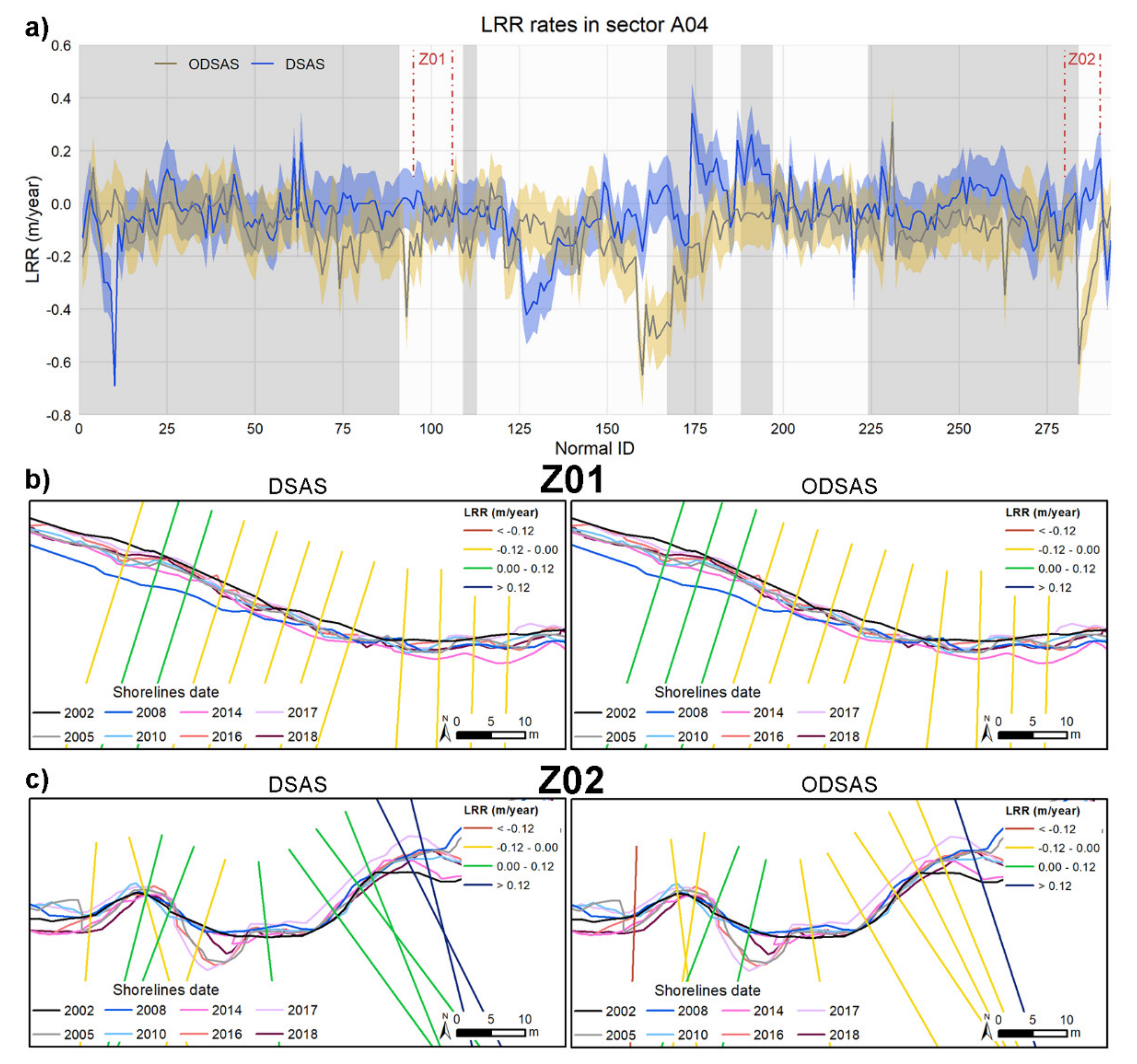
The transect-by-transect comparison showed not only sites for which ODSAS and DSAS are very similar but also other places where differences are significant, as illustrated in Figure 7a for site A04. This figure shows the LLR value and uncertainty buffer for each transect along the coast, obtained using DSAS and ODSAS. The larger the intersection of LRR values and uncertainty buffer, the more similar are the results from both methods. To guide the reader, we have colored in gray those sections that correspond with the curvilinear sections of the baseline and, with a white background, the regions where the baseline is roughly rectilinear. Surprisingly, the largest differences are not found along the curvilinear sections but are instead on the rectilinear ones, for which even the sign of LRR is different (i.e., one method produced negative LRR values, while the other method produced positive values). To better understand this behavior, we have zoomed into two specific areas (Z01, Z02) within the A04 site, for which we show the transects for each method (Figure 7b,c). In Z01, the LRR values from both methods are very similar, with almost identical values and transect orientations. In the case of Z02, the historical coastlines’ longshore variability is greater than Z01, as indicated by the colors of the transects that represent different LRR value ranges. This longshore variability, combined with small differences in the transect orientations, explains the differences between the two methods tested. Differences in the transect starting point and orientation led to the intersection with the shorelines being in different positions, which explains the differences in the distances estimated by each method.

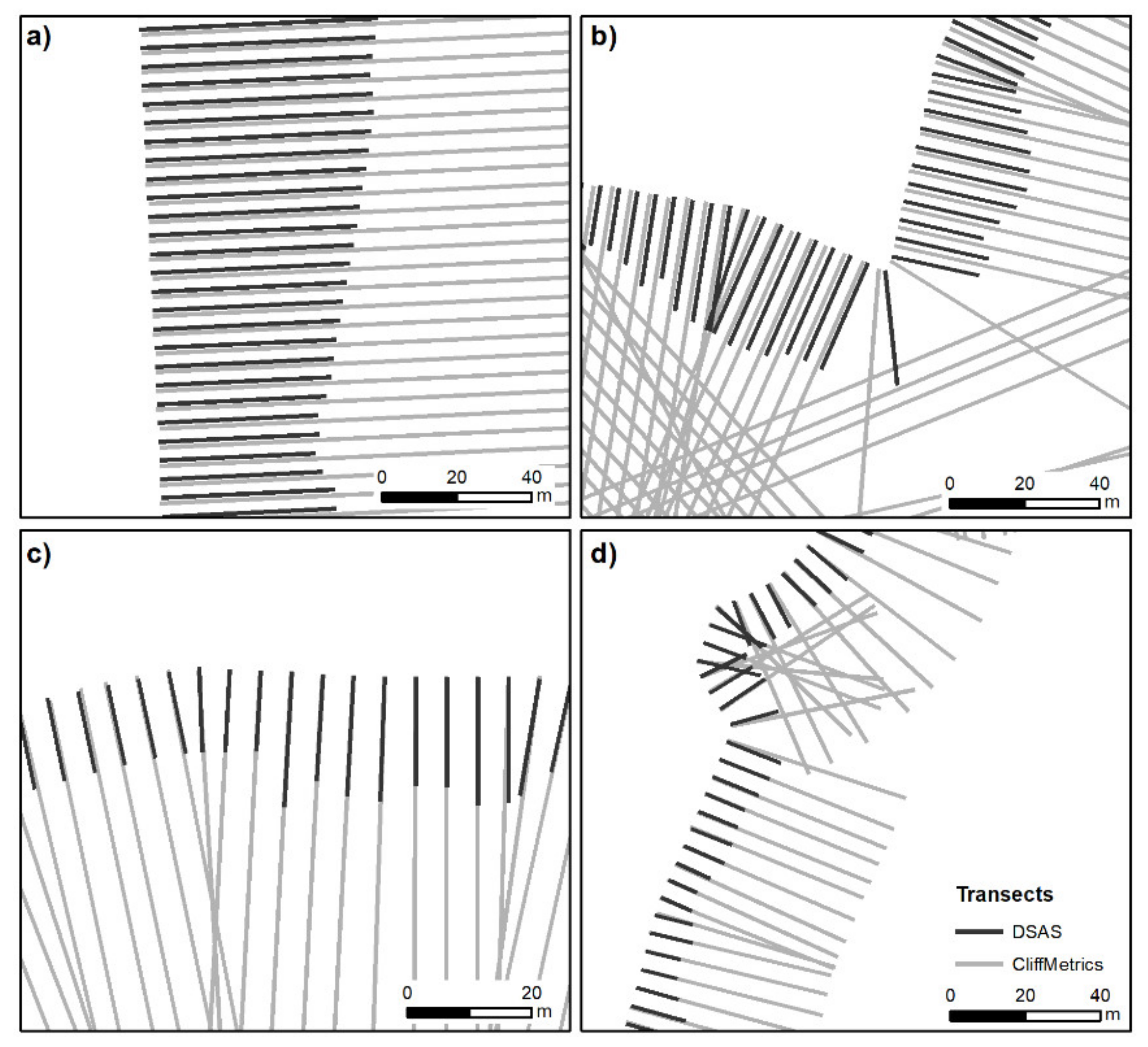
To better understand the differences between the transects generated by DSAS and ODSAS methods, we have compared them for four different coastal geometries in Figure 8. For baselines of a rectilinear or almost rectilinear shape (Figure 8a,c), the orientation of the transects is almost identical, with only small differences in the start of the transects (notice that transects do not overlap but are very close to each other). For baselines with sharp edges or a very irregular shape (Figure 8b,d), we notice that not only the start of the transect but also the orientation of the transects can be significantly different. Which transect is better in particular circumstances is for the user to decide, and is, therefore, subjective.

Table 5. Aggregated mean values of EPR, LRR and WLR, and the number of transects obtained using different baselines in ODSAS for site A04.

Baseline Position	EPR [m yr−1]	LRR [m yr−1]	WLR [m yr−1]	Transects [n]
Offshore [m yr−1]	−0.11	−0.03	−0.09	293
Intermediate * [1]	1.0	1.3	1.2	330
Onshore * [1]	1.1	1.7	1.4	291

* Values shown for Intermediate and Onshore baselines are the ratio of the EPR, LRR, and WLR values obtained, divided by the values obtained using the Offshore baseline.

shows the aggregated mean rates (EPR, LRR, WLR) for all transects for site A04 but using a baseline in various positions: offshore, inland, and at an intermediate location between the previous two. The offshore position is the same as that we used previously; the onshore baseline is designed using the same technique explained in Section 2.3; and, for the intermediate baseline location, we have used the most ancient historical coastline for this site (from 2002, in this case). The number of transects varies with the length of the baseline used, which in this case ranges from 291 to 330. The rate of change for all cases and parameters is similar to the first decimal point. Because the rates of change are small (i.e., absolute values are less than 0.2 m yr⁻¹) the relative differences in the values obtained using an offshore baseline vary from factor 1.0 (EPR-Intermediate vs. Offshore) to 1.7 (LRR-Onshore vs. Offshore).

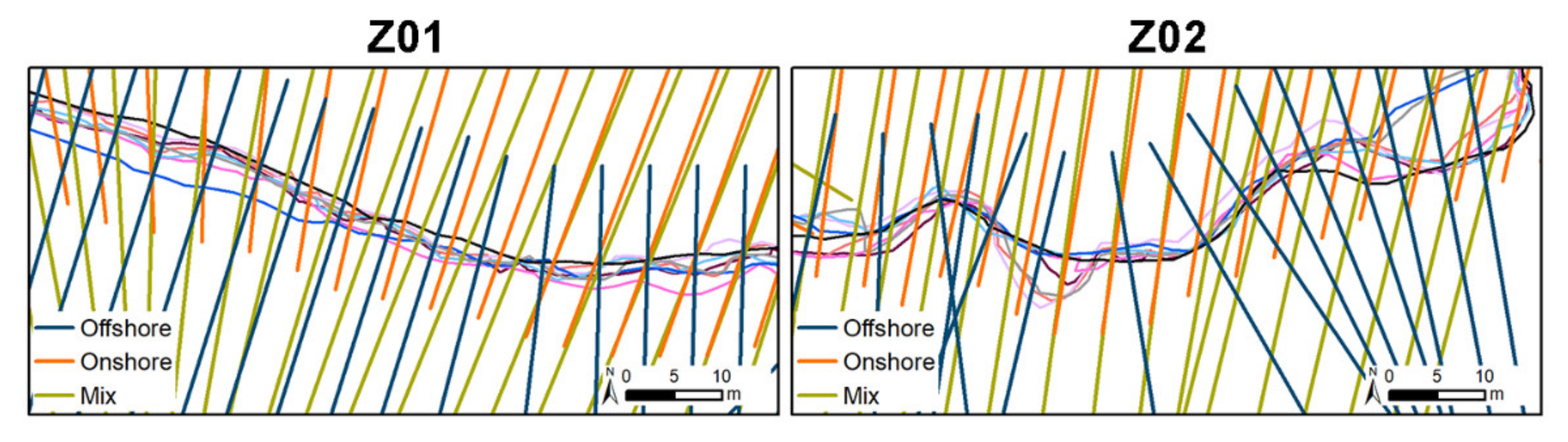
As in the DSAS and ODSAS comparison, the variations between the values obtained when using ODSAS but employing different baselines are related to the transects starting positions and their orientations, as illustrated in Figure 9. In this case, we have represented the three baseline possibilities in the same sectors (Z01, Z02) as shown previously, to explain the differences in site A04. The starting point of each transect in this comparison is different because we are using three different baselines, so the focus is on the transect orientation. In both zoomed sites, the offshore baseline orientation differs significantly from the transect orientation obtained using the other baselines, especially in Z02.

4. Discussion

We argue here that while there is an unavoidable degree of subjectivity when using the baseline transect method to measure coastline change, this can be reduced by explicitly including the spatial resolution as part of the process (Figure 5), which is especially important when assessing very irregular coastlines [27].

Our new “baseline and transect” ODSAS method differs from other existing methods (i.e., DSAS, AMBUR and EPR4Q) in the way that the smoothing determines the transect starting point and orientation by combining raster and vector objects in the process. It is important to begin by noticing that if we use the same transects as used by DSAS, the EPR, NSM, SCE, LRR and WLR are identical and by extension [12] identical to AMBUR and EPR4Q. The differences between the results obtained by ODSAS and DSAS emerge when we use similar but not identical transects, as shown at both aggregated values and at individual transect levels (Table 4 and Figure 7). By requesting that the user inputs a DEM of a given resolution, we are explicitly defining the spatial resolution of the study (e.g., 1 m in our study) and, by using the raster centroid to map the start of the transects, we are also: (1) acknowledging that both the baseline points also have some location uncertainty [20,28]; and (2) constraining the spatial domain in which the transect start can be mapped. In ODSAS, there are N × M potential points on which the transect starting point can be located, where N and M are the numbers of rows and columns of the explicitly defined DEM as an input file. In DSAS, AMBUR and EPR4Q, the transect starting point can be located on a potentially infinite number of locations along the user-defined baseline. While all methods of delineating the transects to a baseline are essentially an abstraction used to measure coastline change, we argue that constraining the transects’ start locations to an explicitly defined DEM resolution is a better fit when comparing shoreline proxies that have been extracted from a digital image. The user, by checking if the number of baseline points is equal to or smaller than the number of transects, now has a numerical indicator of the adequacy of the transect spacing, relative to the resolution of the study.

To the best of our knowledge, there are no other peer-reviewed studies that have assessed the sensitivity of the EPR, NSM, SCE, LRR and WLR values to the transects generation process for very irregular coastlines. Genz [26] analyzed the sensitivity of these values to the window size that was used for smoothing. Konlechner et al. [29] mentioned that there are problems associated with transect generation along very irregular coastlines but did not include quantitative comparisons. A similar approach appeared in [30], where the discussion section explained the relevance of spatial resolution and temporal coverage in the construction of transects. Recently, Nicu [31] analyzed the relevance of transects in gully erosion rates and how different smoothing and spacing parameters are needed to adjust the best transects for each sector.

The proposed ODSAS method is based on free open software (SAGA and R); therefore, the user does not need any license to perform the entire process. SAGA and R are available for all operating systems, and the processes should not cause any problems on different platforms. As an open-source tool, users can modify this method and adapt the codes to their particular aims (e.g., incorporating new coastline change parameters). It is important to highlight that for any tool (e.g., DSAS, AMBUR, EPR4Q or ODSAS) that applies the baseline-transect method, it is necessary to use a GIS environment to work with the historical coastlines and the baseline.

The baseline and transect methodology is an abstraction (i.e., neither the baseline nor transects exist in nature and are therefore subjective) that researchers and practitioners use for SCA. We have shown in this work that the metrics of change are very sensitive not only to the baseline location but also to the way in which the transects are delineated. We conclude that there is no objective rule by which to define the most appropriate positioning for baselines or transect delineation but, as the commonly used metrics of change in SCA are sensitive to both baseline and transect locations, there is also a need to report the baselines and transects used for a particular SCA study, which are not always reported.