Random Forest Modeling of Soil Properties in Saline Semi-Arid Areas

Abstract

The problem of salinization/spreading of saline soils is becoming more urgent in many regions of the world, especially in context of climate change. The monitoring of salt-affected soils’ properties is a necessary procedure in land management and irrigation planning and is aimed to obtain high crop harvest and reduce degradation processes. In this work, a machine learning method was applied for modeling of the spatial distribution of topsoil (0–20 cm) properties—in particular: soil organic carbon (SOC), pH, and salt content (dry residue). A random forest (RF) machine learning approach was used in combination with environmental variables to predict soil properties in a semi-arid area (Trans-Ural steppe zone). Soil, salinity, and texture maps; topography attributes; and remote sensing data (RSD) were used as predictors. The coefficient of determination (R²) and the root mean square error (RMSE) were used to estimate the performance of the RF model. The cross-validation result showed that the RF model achieved an R² of 0.59 and an RMSE of 0.68 for SOM; 0.36 and 0.65, respectively, for soil pH; and 0.78 and 1.21, respectively for dry residue prediction. The SOC content ranged from 0.8 to 2.8%, with an average value of 1.9%; soil pH ranged from 5.9 to 8.4, with an average of 7.2; dry residue varied greatly from 0.04 to 16.8%, with an average value of 1.3%. A variable importance analysis indicated that remote sensing variables (salinity indices and NDVI) were dominant in the spatial prediction of soil parameters. The importance of RSD for evaluating saline soils and their properties is explained by their absorption characteristics/reflectivity in the visible and near-infrared spectra. Solonchak soils are distinguished by a salt crust on the land surface and, as a result, reduced SOC contents and vegetation biomass. However, the change in saline and non-saline soils over a short distance with mosaic structure of soil cover requires high-resolution RSD or aerial images obtained from unmanned aerial vehicle/drones for successful digital mapping of soil parameters. The presented results provide an effective method to estimate soil properties in saline landscapes for further land management/reclamation planning of degraded soils in arid and semi-arid regions.

1. Introduction

Soil salinization is a global land degradation process and environmental problem, especially in arid and semi-arid regions. Furthermore, soil salinity also affects other major land degradation phenomena, such as desertification, soil dispersion, increased soil erosion, and engineering problems [1]. However, among degraded soils, salt-affected soils have a high potential for carbon sequestration in terrestrial ecosystems [2,3]. Currently, about 7% (932.2 Mha [4]) of the world’s land surface is threatened by salinization, which occurs in at least 100 countries [5], with hotspots in Pakistan, China, the United States of America, India, Argentina, Sudan, and many countries in Central and Western Asia [6]. An effective prediction indicates that 50% of the world’s cultivated land will become salt soil by 2050 [7]. In Russia, the area of salt-affected soils in agricultural lands is estimated to be 9% (16.3 Mha), including 11.4 Mha (70.1% of the area of salt-affected soils) of slightly and moderately saline soils [8]. Within Russia, the saline soils are predominantly located in the southern regions. In these regions, agriculture is extensively developed and occupies the most croplands of the country [9].

The genesis of natural salinity is primarily based on physical and/or chemical weathering of salts and their migration from parent material, geologic deposits, or groundwater [10]. However, secondary salinization is mainly caused by external factors, such as irrigation, other agricultural practices, and/or by acidic precipitation [11,12,13,14,15]. Secondary salinization affects ~77 Mha, with 58% of these in irrigated areas. Nearly 20% of all irrigated land is salt-affected, and this proportion tends to increase in spite of considerable efforts dedicated to land reclamation [16]. The above-mentioned factors significantly limit soil fertility and crop productivity, resulting in economic risks and non-benefits. Salinization-related losses in crop production in arid and semi-arid areas of the world range between 18 and 43 percent [17].

With an expected 9 billion people by 2050 and average income on the rise in the developing world, meeting future food demand will be a challenge [18]. It estimated that food production must increase by 38 and 57% by the years 2025 and 2050, respectively [4]. Climate change, urbanization, and land degradation/salinization are putting further pressure on the food supply. Agricultural sustainability strongly depends on the condition of land resources. Despite the development of degradation processes, many agricultural areas continue to be exploited [19,20]. Under such unfavorable circumstances, assessment and monitoring of soil properties—especially on degraded lands—is essential for efficient production of agricultural crops.

Soil salinization is a dynamic process that both complicates the mapping of soil properties [16] and requires periodical field surveys to obtain actual data. The ability to monitor and map spatial distributions of soil salinity and properties has been demonstrated in numerous studies. For example, the most successful method for assessing and mapping salt-affected soils is remote sensing data (RSD), which has proven effectiveness in many parts of the world [21,22,23,24,25]. In general, the success in detecting saline soils is related to the salts on the surface, which strongly correlate with spectral reflectance [16].

Digital soil mapping (DSM) approaches were developed as an alternative to conventional mapping methods because DSM are faster and more cost-effective (not requiring extensive field surveys), could be used in different scales and cover large areas, and showed a high prediction level [26,27,28]. DSM includes a relationship between soil parameters and environmental variables (covariates) [29]. Topographic attributes and RSD are the most popular variables for the digital mapping of soil properties [30]. However, such covariates are sometimes uninformative due to the relatively low spatial resolution for small areas/large-scale objects. Meanwhile, several studies have shown that collocated derived digital maps of soil properties were key variables (instead of environmental variables) for predicting other soil characteristics [31,32,33]. Moreover, soil maps are also one of the most effective sources for spatial prediction of some biophysicochemical soil properties. For example, a number of studies have identified soil maps as the most important covariates for modeling soil organic carbon (SOC) [34,35].

Many researchers have identified clear relationships between the soil salinity, SOC content, soil texture, and moisture, which are also strongly correlated with soil albedo [36]. Thus, soil salinity can be used as an additional explanatory variable for spatial prediction of soil characteristics. Based on this assumption, we tested the possibility of using DSM methods to predict some properties of salt-affected soils. The aims of the present study were to: (i) predict the spatial distribution and values of SOC, pH, and dry residue using the random forest (RF) approach; and (ii) determine the most important variables in the spatial distribution of soil properties under arid/saline conditions.

2. Materials and Methods

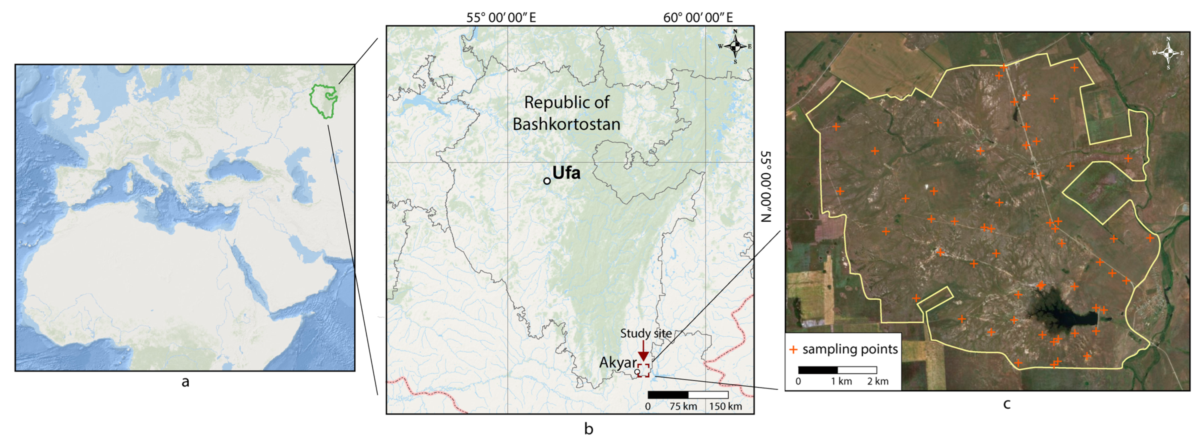
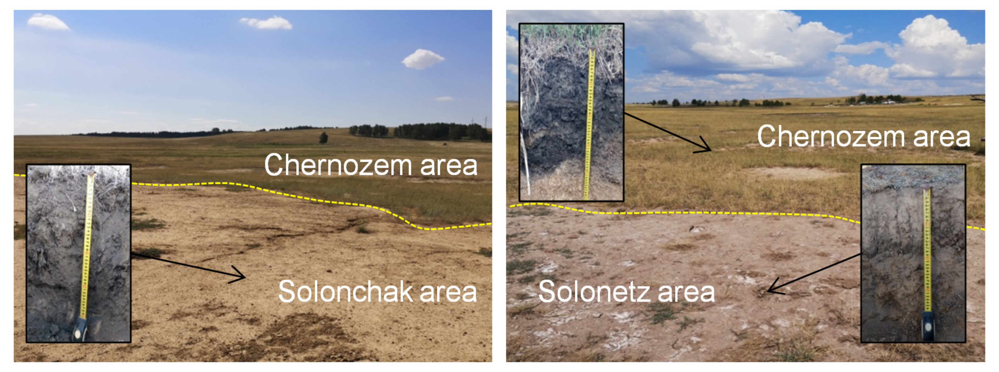
2.1. Study Site Discription

The study area of 5100 ha is located in the Khaybullinsky District (Republic of Bashkortostan (RB), Russia) (Figure 1) and belongs to Trans-Ural steppe zone. According to Pankova et al. [9], this region is classified as the zone of spreading of saline soils within agricultural lands. The total area of hotspots and areals of natural saline soils only in the southern part of RB amounts to ~60 Kha [37]. Elevation in the study site ranges from 300 to 350 m a.s.l. The land use/land cover of the research site is mostly presented by virgin or abandoned agricultural lands. The climate in the study area is moderately warm and arid (Dfb according to the Köppen climate classification [38]), with an average annual precipitation of 316 mm. The mean annual air temperature is 3.8 °C. The mean January temperature is −13.8 °C, and the mean temperature in July is +20.7 °C. The Vysotsky-Ivanov moisture coefficient [39], which is defined as the ratio of the annual precipitation to the annual evaporation, is 0.46 [40] (insufficient moisture supply). The hydrothermal coefficient [41] as a climatic indicator of moisture availability of the territory is 0.71 [40] (arid zone). Over the past 37 years, an increase in the average monthly and annual air temperatures (on 1.4 °C) and a decrease in the amount of precipitation in the summer (on 4.4 mm) was observed for study site [42]. Such continued aridization of the climate accelerates salinization processes and limits land fertility.

The soil cover of the study site is presented by chernozems, solonchaks, and solonetz, according to the WRB classification [43]. Predominant parent materials are diluvial yellow-brown carbonate clays and heavy loams. Salt-affected soils (solonchaks and solonetz) are mostly located in combination with chernozems and do not form large areas, only in same places they found as hotspot areals. The types of salinity of these soils are sulfate, chloride-sulfate, and mixed. The genesis of soil salinization is associated with a high content of water-soluble salts from tertiary seas, mineralized groundwater, and the arid climate. The vegetation is mainly presented by steppe plants and different halophytes (e.g., Volga fescue (Festuca valesiaca), European feather grass (Stipa pennata), picklegrass (Salicornia), etc.).

2.2. Soil Sampling and Laboratory Analyses

The soil sampling was carried out via a stratified random-sampling scheme under dry meteorological conditions (July–August). All soil samples (52) were collected from the topsoil depth (0–20 cm) using a shovel, and their locations were georeferenced by a GPS device. The samples were delivered to the laboratory and then processed (dried, ground, sieved, etc.) for the subsequent chemical analyses. SOC content was determined via a wet combustion method [44]. The gradation of the SOC on the categories was carried out according to the scale [45], on which content >5.8% is characterized as “very high”, 3.5–5.8 is “high”, 2.3–3.5 is “average”, 1.4–2.3 is “low”, and <1.4 is “very low”. Soil reaction was measured potentiometrically in H₂O suspension with a soil–water ratio of 1:2.5. The total content of water-soluble salts (dry residue) of soil was determined by evaporation of 1:5 soil–water extracts.

2.3. Environmental Covariates

Environmental variables for the digital mapping of soil properties are presented in

Table A1. Environmental variables used for spatial modeling.

Environmental Variable	Environmental Parameters	Acronym	Equation for Sentinel-2A	Source
Spectral indices	Salinity index 1	SI1	$\sqrt{\mathrm{B}2\times \mathrm{B}4}$	[63]
	Salinity index 2	SI2	$\sqrt{\mathrm{B}3\times \mathrm{B}4}$	[63]
	Salinity index 3	SI3	$\sqrt{{\left(\mathrm{B}3\right)}^2+{\left(\mathrm{B}4\right)}^2+{\left(\mathrm{B}8\right)}^2}$	[64]
	Salinity index 4	SI4	$\sqrt{{\left(\mathrm{B}3\right)}^2+{\left(\mathrm{B}4\right)}^2}$	[64]
	Salinity index I	S1	$\frac{\mathrm{B}2}{\mathrm{B}4}$	[11,65]
	Salinity index II	S2	$\frac{\mathrm{B}2-\mathrm{B}4}{\mathrm{B}2+\mathrm{B}4}$	[11,65]
	Salinity index III	S3	$\frac{\mathrm{B}3\times \mathrm{B}4}{\mathrm{B}2}$	[11,65]
	Salinity index IV	S4	$\frac{\mathrm{B}2\times \mathrm{B}4}{\mathrm{B}3}$	[65]
	Salinity index V	S5	$\frac{\mathrm{B}4\times \mathrm{B}8}{\mathrm{B}3}$	[65]
	Salinity index VI	S6	$\frac{\mathrm{B}3+\mathrm{B}4+\mathrm{B}8}{2}$	[64]
	Salinity index VII	S7	$\frac{\mathrm{B}3+\mathrm{B}4}{2}$	[64]
	Salinity index VIII	S8	$\frac{\mathrm{B}11-\mathrm{B}12}{\mathrm{B}11+\mathrm{B}12}$	[66]
	Salinity index IX	S9	$\frac{\mathrm{B}11}{\mathrm{B}12}$	[66]
	Normalized difference vegetation index	NDVI	$\frac{\mathrm{B}8-\mathrm{B}4}{\mathrm{B}8+\mathrm{B}4}$	[67]
	Normalized difference salinity index	NDSI	$\frac{\mathrm{B}4-\mathrm{B}8}{\mathrm{B}4+\mathrm{B}8}$	[63]
Terrain data	Elevation	DEM		SRTM
	Aspect	Aspect		SAGA GIS
	Multiresolution ridge top flatness	MrRTF		SAGA GIS
	Multiresolution valley bottom flatness	MrVBF		SAGA GIS
	Slope	Slope		SAGA GIS
	Plan curvature	Plan_Cur		SAGA GIS
	Profile curvature	Profile_Cur		SAGA GIS
Maps	Salinity	Salinity map		[46]
	Texture	Texture map		-
	Soil	Soil map		-

. To explain and estimate the spatial distribution of SOC, pH, and dry residue, we selected an environmental parameter including terrain attributes, spectral indices derived from satellite, maps of soil, salinity, and texture. A 30 m digital elevation model (DEM) was used to derive topographic attributes, namely elevation, slope, aspect, plan curvature, profile curvature, multiresolution ridge top flatness (MrRTF), and multiresolution valley bottom flatness (MrVBF) indices. The spectral indices were obtained from the Sentinel-2A satellite image scene covering the study area contemporaneous with the soil sampling period. We used the normalized difference vegetation index (NDVI) and 14 salinity indices. The generated salinity map based on RSD was used for digital mapping [46]. All environmental variables were presented in raster format and coordinate system WGS 84/World Mercator (EPSG:3395).

2.4. Machine Learning Approach

In the present study, the RF approach was applied to predict the spatial patterns of soil properties. RF is the extension of the CART (Classification and Regression Tree analysis) method developed by Breimen [47] and the most popular algorithm in DSM [48]. RF consists of numerous individual tree models trained from bootstrap samples of the data and allows identification of the importance of the variables used compared to linear regression. The results of all individual trees are aggregated to make a single prediction. The RF approach was also discovered to be the most suitable for a small number of samples or data (<100) [49]. The main parameters in this model are the number of predictors (mtry) and the number of trees to be built in the forest (ntree). These parameters were adjusted to obtain the best performance from the model. To select the most important predictors, we applied the recursive feature elimination algorithm for each RF model used. The algorithm works by performing backward selection, in which the least promising predictors are excluded from the model based on an initial predictor importance measure.

2.5. Validation and Statistical Analyses

We applied a leave-one-out cross-validation (LOOCV) approach to evaluate the prediction performance of the RF model. LOOCV is appropriate for a small dataset and consists of using all training data, leaving one out. The coefficient of determination (R²) and root mean squared error (RMSE) were used to validate the spatial prediction accuracy. In general, high R² and a low RMSE values indicate a better level of model prediction. The R² and RMSE are defined as:

$$R^2={\left(\frac{{{\displaystyle \sum }}_{i=0}^n\left(O_i-O_{avg}\right)\times \left(P_i-P_{avg}\right)}{\sqrt{{{\displaystyle \sum }}_{i=0}^n{\left(O_i-O_{avg}\right)}^2}\times {\left(P_i-P_{avg}\right)}^2}\right)}^2$$

(1)

$$\mathrm{RMSE}=\sqrt{\frac{{{\displaystyle \sum }}_{i=0}^n{\left(O_i-P_i\right)}^2}{n}}$$

(2)

where O_i and P_i are observed and predicted values of soil properties, respectively; n is the number of samples.

The variability of soil properties was assessed according to the scale [50], on which coefficient of variation (CV) values <15% is classified as “low”, 15–35%—“moderate”, and >35%—“high”. The statistical analysis, spatial modeling, and cross-validation were performed in R 4.0.4 and RStudio.

3. Results

3.1. Descriptive Statistics

Summary statistics of soil properties in the study plot are presented in

Table 1. Descriptive statistics of studied soil properties.

Soil Parameter	Min	Max	Mean	Median	SD	CV, %
n = 52
SOC, %	0.8	2.8	1.9	1.9	0.5	27.3
pH H2O	5.9	8.4	7.2	7.4	0.7	9.8
Dry residue, %	0.04	16.8	1.3	0.2	3.4	257.8

Notes: n—number of samples; SD—standard deviation; CV—coefficient of variation.

. At the 0–20 cm depth, the SOC content varied from 0.8 to 2.8%, with a mean value of 1.9%. The SOC content according to the categories ranged from “very low” (<1.2%) to “average” (2.3–3.5%), while the SOC mean value was “low”. The CV value for SOC content indicated a moderate variability (27.3%). The soil reaction (pH) ranged from near-neutral to highly alkaline (5.9–8.4), while the average pH value was classified as alkaline (7.2). The soil pH variability was characterized as “low” (9.8%). The dry residue content varied over a wide range (0.04–16.8%) and had a “very high” CV value (257.8%), which is explained by different soil types in terms of salinity.

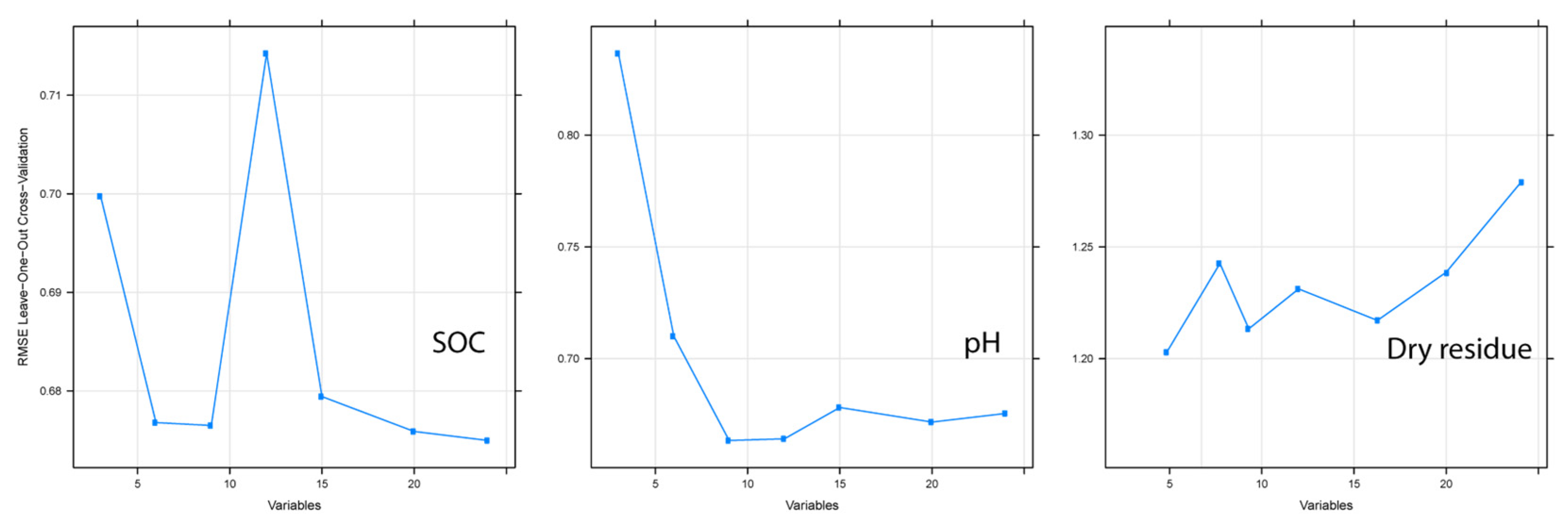
3.2. Performance of RF Model and Optimal Number of Environmental Covariates

Table 2. Predictive quality of RF in soil properties modeling.

Soil Parameter	R2	RMSE
SOM, %	0.59	0.68
pH H2O	0.36	0.65
Dry residue, %	0.78	1.21

presents the evaluation of modeling according to the error indices (R² and RMSE). According to the R², the most accurate spatial estimate was found for the dry residue content (R² = 0.78, RMSE = 1.21). The indices R² and RMSE of the SOC modeling were 0.59 and 0.68, respectively, and 0.36 and 0.65, respectively, for the soil pH.

Figure 2 shows the optimal number of environmental variables used in the RF prediction of SOC, pH, and dry residue according to the RMSE metric. The variable selection in the recursive feature elimination procedure showed that all environmental variables were not important covariates for predicting soil properties. The optimal number of covariates included in the RF predictive model for SOC was 20, while the optimal numbers were 9 and 5 for soil pH and dry residue, respectively.

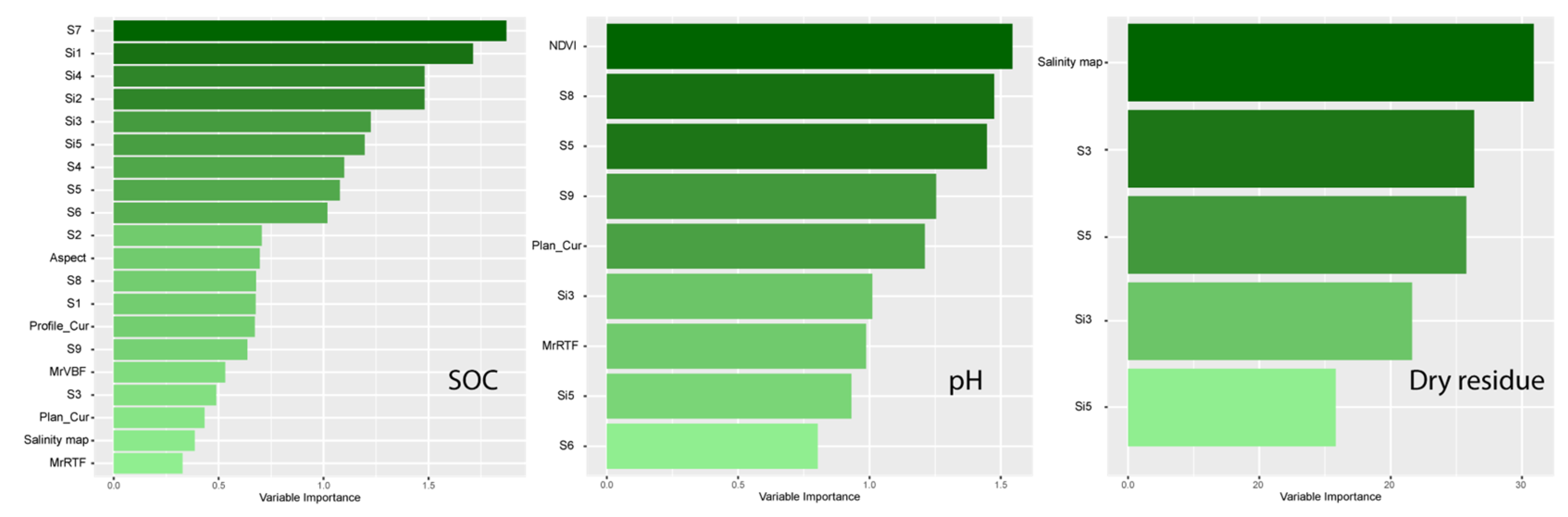
3.3. Variable Importance Assessment of RF Model

Figure 3 shows the relative importance and contribution of the environmental variables in the spatial prediction of SOC, pH, and dry residue. The results showed that the best explanatory variables for the SOC modeling were salinity indices derived from Sentinel-2A data. In descending order, the indices S7, Si1, Si4, Si2, Si3, Si5, S4, S5, S6, and S2 were important for the spatial modeling of SOC content. NDVI, salinity indices, and two terrain attributes (plan curvature and MrRTF) were identified as the most important variables in the RF for modeling soil pH. According to the RF model, the spatial distribution of dry residue was determined by the salinity map and salinity indices (S3, S5, Si4, and Si5). In general, remote sensing indices were the top variables in the spatial prediction of all soil properties using the RF model.

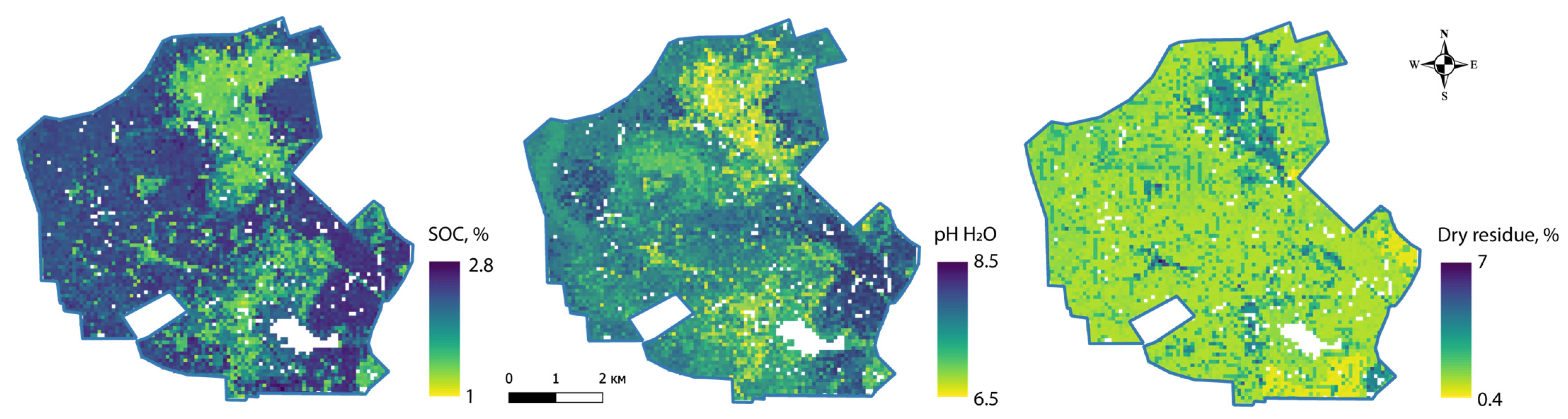
3.4. Generated Maps Using the RF Model

Figure 4 shows the digital maps of SOC, soil pH, and dry residue using the RF method. Predicted average SOC values ranged from 1 to 2.8%, pH values from 6.5 to 8.5 and dry residue from 0.4 to 7%. The generated maps indicated a “low” SOC content dominantly located in the southern and northern parts of the study area, while a “high” SOC content was mostly found randomly in the other parts. The higher concentrations of dry residue were observed in the northern and southern parts around the reservoir (located in the northern part of study site; water surface is painted dark blue in Figure 1c and white in Figure 4).

4. Discussion

The research site is distinguished by frequent changes and short distance variability of soil types within the landscape (Figure 5). This phenomenon is common in arid and semi-arid zones and for soil cover affected by salts. Where a large concentration of salts occupies topsoil layer and/or a salt crust on the soil surface appears, the solonchaks are formed. This soil type does not occupy large areas and formed only small areals nearby with solonetz and chernozems. Thus, the salts—in addition to the main factors of soil formation (relief, parent material, organisms, climate, and time) [51]—have a great influence on the development of soil types and soil properties spatial distribution [52]. Since salinity reduces plant growth/productivity, i.e., carbon input to the soil, the SOC content in saline soils (especially in the 0–20 cm layer of solonchaks) is often lower than in adjacent soils. This is also evidenced by the compiled maps (Figure 4), which trace the relationship between soil properties.

In this study, the key variables for spatial prediction of soil properties were soil salinity indices derived from RSD. The spectral indices explain the spatial distribution of soil properties well [30,42,53,54], and they are crucial for modeling in saline landscapes [55]. This occurs because salt-affected soils have clear reflectivity and absorption characteristics in the visible and near-infrared spectra [56]. Thus, soils that have a salt crust can be identified and mapped. Topographic attributes were not recognized as most important for modeling soil properties. Previously, Peng et al. [55] used a cubist machine learning approach to evaluate the spatial variability of soil salinity and discovered that terrain data contributed less to spatial prediction than RSD. Nabiollahi et al. [57] used RF approach to estimate the spatial distribution of soil pH, electrical conductivity, and sodium adsorption ratio on agricultural salt-affected land. Results showed that the most important covariates were groundwater table, categorical maps, salinity index, and MrRTF. In our study, the lower SOC contents on the produced digital maps were also found around the reservoir, which is explained by the close proximity of the groundwater level. Since the genesis of the studied saline soils is associated with groundwater evapotranspiration, it can be assumed that groundwater level maps can significantly improve the spatial prediction results.

Because RSD are critical for the digital mapping of salt-affected soils and their characteristics, greater emphasis attention should be placed on the spatial resolution of satellite imagery. Perhaps in this study, spatial resolution of spectral indices hampered the RF model performance because the images were unable to depict the frequent change in soil types over a short distance. Due to the mosaic structure of the soil cover, high- and ultra-high-resolution (<10 m) remote sensing or unmanned aerial data are required, while medium- and small-scale images are unable to present such circumstances. At the same time, it can be assumed that an increase in the density and number of sampling points is important for DSM in a heterogeneous landscape, especially subjected to erosional processes [58].

Global ecosystems are severely impacted by climate change. Increasing average annual temperatures and decreasing precipitation have a leading influence on salinization processes in arid and semi-arid regions [59]. Previously, numerous studies have demonstrated changes in climatic indicators in the Ural region [42,60,61,62], which contribute to soil salinity. As previously mentioned, the key factor driving soil salinization in the research region is groundwater level/table. Thus, fluctuations in the level of groundwater during climate change will contribute to the formation of both solonchaks and solonetzic soils.

5. Conclusions

In the steppe zone of Southern Ural, under the conditions of changing climate (aridization), the risk of increases in area and salinization degree of saline soils are rising. Therefore, it is necessary to monitor soil properties and update maps to take preventive measures in applied land management practices aimed at reducing soil degradation processes and increasing crop yield. Machine learning tools could be used as useful alternative and additional methods to traditional soil property monitoring/mapping and could minimize field surveys, labor, and time cost. The random forest (RF) approach used showed its effectiveness, i.e., moderate and high levels of prediction, in the modeling of spatial soil property distribution. In particular, the error indices (R² and RMSE) were 0.59 and 0.68, respectively, for the SOC modeling; 0.36 and 0.65, respectively, for pH; and 0.78 and 1.12, respectively for salt content. Salinity indices and NDVI derived from remote sensing data (RSD) were found to be the best environmental variables in the prediction modeling of soil properties among terrain attributes and soil type/salinity/texture maps. Since the presence of salts on the soil surface in most cases indicated a lower SOC content, the spectral reflectance of salt-affected soils was crucial for successful SOC modeling. However, the alternation of saline soils (solonchaks and solonetz) and nonsaline (chernozems) in the study area reduced the efficiency of the RF model. Therefore, improved spatial prediction of soil properties should be achieved with high-resolution images obtained from RSD or unmanned aerial vehicles/drones. In addition, because the formation of saline soils is related to the level/table of groundwater and the amount of salts in it, such maps should be used to obtain a more accurate spatial prediction.

References

1. Li, P.; Wu, J.; Qian, H. Regulation of secondary soil salinization in semi-arid regions: A simulation research in the Nanshantaizi area along the Silk Road, northwest China. Environ. Earth Sci. 2016, 75, 698. [Google Scholar] [CrossRef]
2. Lal, R. Potential of desertification control to sequester carbon and mitigate the greenhouse effect. Clim. Chang. 2001, 51, 35–72. [Google Scholar] [CrossRef]
3. Setia, R.; Gottschalk, P.; Smith, P.; Marschner, P.; Baldock, J.; Setia, D.; Smith, J. Soil salinity decreases global soil organic carbon stocks. Sci. Total Environ. 2013, 465, 267–272. [Google Scholar] [CrossRef] [PubMed]
4. Rengasamy, P. World salinization with emphasis on Australia. J. Exp. Bot. 2006, 57, 1017–1023. [Google Scholar] [CrossRef] [PubMed]
5. Qadir, M.; Noble, A.D.; Schubert, S.; Thomas, R.J.; Arslan, A. Sodicity-induced land degradation and its sustainable management: Problems and prospects. Land Degrad. Dev. 2006, 17, 661–676. [Google Scholar] [CrossRef]
6. Cuevas, J.; Daliakopoulos, I.N.; del Moral, F.; Hueso, J.J.; Tsanis, I.K. A review of soil-improving cropping systems for soil salinization. Agronomy 2019, 9, 295. [Google Scholar] [CrossRef]
7. Butcher, K.; Wick, A.F.; DeSutter, T.; Chatterjee, A.; Harmon, J. Soil salinity: A threat to global food security. Agron. J. 2016, 108, 2189–2200. [Google Scholar] [CrossRef]
8. Khitrov, N.B.; Rukhovivh, D.I.; Kalinina, N.V.; Novikova, A.F.; Pankova, E.I.; Chernousenko, G.I. Estimation of the areas of salt-affected soils in the European part of Russia on the basis of a digital map of soil salinization on a scale of 1:2.5 M. Eurasian Soil Sci. 2009, 42, 581–590. [Google Scholar] [CrossRef]
9. Pankova, E.I. Salt-affected soils of Russia: Solved and unsolved problems. Eurasian Soil Sci. 2015, 48, 115–127. [Google Scholar] [CrossRef]
10. Daliakopoulos, I.N.; Tsanis, I.K.; Koutroulis, A.; Kourgialas, N.N.; Varouchakis, A.E.; Karatzas, G.P.; Ritsema, C.J. The threat of soil salinity: A European scale review. Sci. Total Environ. 2016, 573, 727–739. [Google Scholar] [CrossRef]
11. Abbas, A.; Khan, S.; Hussain, N.; Hanjra, M.A.; Akbar, S. Characterizing soil salinity in irrigated agriculture using a remote sensing approach. Phys. Chem. Earth Parts A/B/C 2013, 55–57, 43–52. [Google Scholar] [CrossRef]
12. Gabbasova, I.M.; Suleimanov, R.R. Transformation of gray forest soils upon technogenic salinization and alkalization and subsequent rehabilitation in oil-producing regions of the southern Urals. Eurasian Soil Sci. 2007, 40, 1000–1007. [Google Scholar] [CrossRef]
13. Gao, Y.; Wang, J.; Guo, S.; Hu, Y.-L.; Li, T.; Mao, R.; Zeng, D.-H. Effects of salinization and crude oil contamination on soil bacterial community structure in the Yellow River Delta region, China. Appl. Soil Ecol. 2015, 86, 165–173. [Google Scholar] [CrossRef]
14. Li, X.; Wang, X.; Zhang, Y.; Zhao, Q.; Yu, B.; Li, Y.; Zhou, Q. Salinity and conductivity amendment of soil enhanced the bioelectrochemical degradation of petroleum hydrocarbons. Sci. Rep. 2016, 6, 32861. [Google Scholar] [CrossRef] [PubMed]
15. Mohanavelu, A.; Naganna, S.R.; Al-Ansari, N. Irrigation induced salinity and sodicity hazards on soil and groundwater: An overview of its causes, impacts and mitigation strategies. Agriculture 2021, 11, 983. [Google Scholar] [CrossRef]
16. Metternicht, G.I.; Zinck, J.A. Remote sensing of soil salinity: Potentials and constraints. Remote Sens. Environ. 2003, 85, 1–20. [Google Scholar] [CrossRef]
17. Wichelns, D.; Qadir, M. Achieving sustainable irrigation requires effective management of salts, soil salinity, and shallow groundwater. Agric. Water Manag. 2015, 157, 31–38. [Google Scholar] [CrossRef]
18. Lenaerts, B.; Collard, B.C.Y.; Demont, M. Review: Improving global food security through accelerated plant breeding. Plant Sci. 2019, 287, 110207. [Google Scholar] [CrossRef]
19. Akramkhanov, A.; Brus, D.J.; Walvoort, D.J.J. Geostatistical monitoring of soil salinity in Uzbekistan by repeated EMI surveys. Geoderma 2014, 213, 600–607. [Google Scholar] [CrossRef]
20. Eisele, A.; Chabrillat, S.; Hecker, C.; Hewson, R.; Lau, I.C.; Rogass, C.; Segl, K.; Cudahy, T.J.; Udelhoven, T.; Hostert, P.; et al. Advantages using the thermal infrared (TIR) to detect and quantify semi-arid soil properties. Remote Sens. Environ. 2015, 163, 296–311. [Google Scholar] [CrossRef]
21. Abuelgasim, A.; Ammad, R. Mapping soil salinity in arid and semi-arid regions using Landsat 8 OLI satellite data. Remote Sens. Appl. Soc. Environ. 2019, 13, 415–425. [Google Scholar] [CrossRef]
22. Ivushkin, K.; Bartholomeus, H.; Bregt, A.K.; Pulatov, A. Satellite thermography for soil salinity assessment of cropped areas in Uzbekistan. Land Degrad. Dev. 2017, 28, 870–877. [Google Scholar] [CrossRef]
23. Hoa, P.V.; Giang, N.V.; Binh, N.A.; Hai, L.V.H.; Pham, T.-D.; Hasanlou, M.; Tien Bui, D. Soil salinity mapping using SAR Sentinel-1 data and advanced machine learning algorithms: A case study at Ben Tre province of the Mekong River delta (Vietnam). Remote Sens. 2019, 11, 128. [Google Scholar] [CrossRef]
24. Melendez-Pastor, I.; Navarro-Pedreño, J.; Koch, M.; Gómez, I. Applying imaging spectroscopy techniques to map saline soils with ASTER images. Geoderma 2010, 158, 55–65. [Google Scholar] [CrossRef]
25. Moreira, L.C.J.; Teixeira, A.d.S.; Galvão, L.S. Potential of multispectral and hyperspectral data to detect saline-exposed soils in Brazil. GIScience Remote Sens. 2015, 52, 416–436. [Google Scholar] [CrossRef]
26. Zeraatpisheh, M.; Jafari, A.; Bodaghabadi, M.B.; Ayoubi, S.; Taghizadeh-Mehrjardi, R.; Toomanian, N.; Kerry, R.; Xu, M. Conventional and digital soil mapping in Iran: Past, present, and future. Catena 2020, 188, 104424. [Google Scholar] [CrossRef]
27. Fantappiè, M.; L’Abate, G.; Schillaci, C.; Costantini, E.A. Digital soil mapping of Italy to map derived soil profiles with neural networks. Geoderma Reg. 2023, 32, e00619. [Google Scholar] [CrossRef]
28. Lozbenev, N.; Komissarov, M.; Zhidkin, A.; Gusarov, A.; Fomicheva, D. Comparative assessment of digital and conventional soil mapping: A case study of the Southern Cis-Ural region, Russia. Soil Syst. 2022, 6, 14. [Google Scholar] [CrossRef]
29. McBratney, A.B.; Mendonça Santos, M.L.; Minasny, B. On digital soil mapping. Geoderma 2003, 117, 3–52. [Google Scholar] [CrossRef]
30. Mulder, V.L.; de Bruin, S.; Schaepman, M.E.; Mayr, T.R. The use of remote sensing in soil and terrain mapping—A review. Geoderma 2011, 162, 1–19. [Google Scholar] [CrossRef]
31. Pahlavan-Rad, M.R.; Dahmardeh, K.; Brungard, C. Predicting soil organic carbon concentrations in a low relief landscape, eastern Iran. Geoderma Reg. 2018, 15, e00195. [Google Scholar] [CrossRef]
32. Tziachris, P.; Aschonitis, V.; Chatzistathis, T.; Papadopoulou, M. Assessment of spatial hybrid methods for predicting soil organic matter using DEM derivatives and soil parameters. Catena 2019, 174, 206–216. [Google Scholar] [CrossRef]
33. Were, K.; Bui, D.T.; Dick, Ø.B.; Singh, B.R. A comparative assessment of support vector regression, artificial neural networks, and random forests for predicting and mapping soil organic carbon stocks across an Afromontane landscape. Ecol. Indic. 2015, 52, 394–403. [Google Scholar] [CrossRef]
34. Gomes, L.C.; Faria, R.M.; de Souza, E.; Veloso, G.V.; Schaefer, C.E.G.R.; Filho, E.I.F. Modelling and mapping soil organic carbon stocks in Brazil. Geoderma 2019, 340, 337–350. [Google Scholar] [CrossRef]
35. Szatmári, G.; Pásztor, L.; Heuvelink, G.B.M. Estimating soil organic carbon stock change at multiple scales using machine learning and multivariate geostatistics. Geoderma 2021, 403, 115356. [Google Scholar] [CrossRef]
36. Nawar, S.; Buddenbaum, H.; Hill, J. Digital mapping of soil properties using multivariate statistical analysis and ASTER data in an arid region. Remote Sens. 2015, 7, 1181–1205. [Google Scholar] [CrossRef]
37. Khaziev, F.K. Soils of Bashkortostan. Volume 1. Ecologic-Genetic and Agroproductive Characterization; Gilem: Ufa, Russia, 1995; p. 385. (In Russian) [Google Scholar]
38. Beck, H.E.; Zimmermann, N.E.; McVicar, T.R.; Vergopolan, N.; Berg, A.; Wood, E.F. Present and future Köppen-Geiger climate classification maps at 1–km resolution. Sci. Data 2018, 5, 180–214. [Google Scholar] [CrossRef]
39. Vysotskii, G.N. Izbrannye Trudy (Selected Works); Sel’khozgiz: Moscow, Russia, 1960; 435p. [Google Scholar]
40. Galimova, R.G.; Perevedentsev, Y.P.; Yamanaev, G.A. Agro-climatic resources of the Republic of Bashkortostan. Vestn. Voronezh. Gos. Univ. Ser. Geogr. Geoekol. 2019, 3, 29–39. (In Russian) [Google Scholar]
41. Selyaninov, G.T. Methods of agricultural climatology. Agric. Meteorol. 1930, 22, 4–20. [Google Scholar]
42. Suleymanov, A.; Gabbasova, I.; Suleymanov, R.; Komissarov, M.; Garipov, T.; Sidorova, L.; Nazyrova, F. The retrospective monitoring of soils under conditions of climate change in the Trans-Ural region (Russia). J. Water Land Dev. 2022, 55, 84–90. [Google Scholar] [CrossRef]
43. IUSS Working Group WRB. World Reference Base for Soil Resources 2014, Update 2015. In International Soil Classification System for Naming Soils and Creating Legends for Soil Maps; World Soil Resources Reports No. 106; FAO: Rome, Italy, 2015. [Google Scholar]
44. Walkley, A.J.; Black, I.A. Estimation of soil organic carbon by the chromic acid titration method. Soil Sci. 1934, 37, 29–38. [Google Scholar] [CrossRef]
45. Semenov, V.; Kohut, B. Soil Organic Matter; GEOS: Moscow, Russia, 2015; ISBN 978-5-89118-702-3. (In Russian) [Google Scholar]
46. Suleymanov, A.; Gabbasova, I.; Abakumov, E.; Kostecki, J. Soil salinity assessment from satellite data in the Trans-Ural steppe zone (Southern Ural, Russia). Soil Sci. Ann. 2021, 72, 132233. [Google Scholar] [CrossRef]
47. Breiman, L. Random Forests. Mach. Learn. 2001, 45, 5–32. [Google Scholar] [CrossRef]
48. Wadoux, A.M.J.-C.; Minasny, B.; McBratney, A.B. Machine learning for digital soil mapping: Applications, challenges and suggested solutions. Earth Sci. Rev. 2020, 210, 103359. [Google Scholar] [CrossRef]
49. Khaledian, Y.; Miller, B.A. Selecting appropriate machine learning methods for digital soil mapping. Appl. Math. Model. 2020, 81, 401–418. [Google Scholar] [CrossRef]
50. Wilding, L.P. Spatial variability: Its documentation, accommodation and implication to soil surveys. In Soil Spatial Variability; Nielsen, D.R., Bouma, J., Eds.; Pudoc: Wageningen, The Netherlands, 1985; pp. 166–194. [Google Scholar]
51. Dokuchaev, V.V. Our Steppes—At One Time and Now; Yevdokimoff Press: St. Petersburg, Russia, 1892. (In Russian) [Google Scholar]
52. Su, Y.; Li, T.; Cheng, S.; Wang, X. Spatial distribution exploration and driving factor identification for soil salinisation based on geodetector models in coastal area. Ecol. Eng. 2020, 156, 105961. [Google Scholar] [CrossRef]
53. Dharumarajan, S.; Hegde, R.; Singh, S.K. Spatial prediction of major soil properties using Random Forest techniques—A case study in semi-arid tropics of South India. Geoderma Reg. 2017, 10, 154–162. [Google Scholar] [CrossRef]
54. Lu, Q.; Tian, S.; Wei, L. Digital mapping of soil pH and carbonates at the European scale using environmental variables and machine learning. Sci. Total Environ. 2023, 856, 159171. [Google Scholar] [CrossRef] [PubMed]
55. Peng, J.; Biswas, A.; Jiang, Q.; Zhao, R.; Hu, J.; Hu, B.; Shi, Z. Estimating soil salinity from remote sensing and terrain data in southern Xinjiang Province, China. Geoderma 2019, 337, 1309–1319. [Google Scholar] [CrossRef]
56. Sidike, A.; Zhao, S.; Wen, Y. Estimating soil salinity in Pingluo County of China using QuickBird data and soil reflectance spectra. Int. J. Appl. Earth Obs. Geoinf. 2014, 26, 156–175. [Google Scholar] [CrossRef]
57. Nabiollahi, K.; Taghizadeh-Mehrjardi, R.; Shahabi, A.; Heung, B.; Amirian-Chakan, A.; Davari, M.; Scholten, T. Assessing agricultural salt-affected land using digital soil mapping and hybridized random forests. Geoderma 2021, 385, 114858. [Google Scholar] [CrossRef]
58. Suleymanov, A.; Polyakov, V.; Komissarov, M.; Suleymanov, R.; Gabbasova, I.; Garipov, T.; Saifullin, I.; Abakumov, E. Biophysicochemical properties of the eroded southern chernozem (Trans-Ural Steppe, Russia) with emphasis on the 13C NMR spectroscopy of humic acids. Soil Water Res. 2022, 17, 222–231. [Google Scholar] [CrossRef]
59. Corwin, D.L. Climate change impacts on soil salinity in agricultural areas. Eur. J. Soil Sci. 2021, 72, 842–862. [Google Scholar] [CrossRef]
60. Bogdan, E.; Kamalova, R.; Suleymanov, A.; Belan, L.; Tuktarova, I. Changing climatic indicators and mapping of soil temperature using Landsat data in the Yangan-Tau UNESCO Global Geopark. SOCAR Proc. 2022, 32–41. [Google Scholar] [CrossRef]
61. Shikhov, A.N.; Abdullin, R.K.; Tarasov, A.V. Mapping temperature and precipitation extremes under changing climate (on the example of The Ural region, Russia). Geogr. Environ. Sustain. 2020, 13, 154–165. [Google Scholar] [CrossRef]
62. Sobol, N.V.; Gabbasova, I.M.; Komissarov, M.A. Impact of climate changes on erosion processes in Republic of Bashkortostan. Arid Ecosyst. 2015, 5, 216–221. [Google Scholar] [CrossRef]
63. Khan, N.M.; Rastoskuev, V.V.; Sato, Y.; Shiozawa, S. Assessment of hydrosaline land degradation by using a simple approach of remote sensing indicators. Agric. Water Manag. 2005, 77, 96–109. [Google Scholar] [CrossRef]
64. Douaoui, A.E.K.; Nicolas, H.; Walter, C. Detecting salinity hazards within a semiarid context by means of combining soil and remote-sensing data. Geoderma 2006, 134, 217–230. [Google Scholar] [CrossRef]
65. Abbas, A.; Khan, S. Using remote sensing techniques for appraisal of irrigated soil salinity. In Proceedings of the Advances and Applications for Management and Decision Making Land, Water and Environmental Management: Integrated Systems for Sustainability MODSIM07, Christchurch, New Zealand, 10–13 December 2007; Modelling and Simulation Society of Australia and New Zealand: Christchurch, New Zealand, 2007; pp. 2632–2638. [Google Scholar]
66. Bouaziz, M.; Matschullat, J.; Gloaguen, R. Improved remote sensing detection of soil salinity from a semi-arid climate in Northeast Brazil. Comptes Rendus Geosci. 2011, 343, 795–803. [Google Scholar] [CrossRef]
67. Rouse, J.W.; Haas, R.H.; Schell, J.A.; Deering, D.W. Monitoring vegetation systems in the Great Plains with ERTS. NASA Spec. Publ. 1974, 351, 309. [Google Scholar]
Figure 1. Locations: (a) the RB in the eastern part of northern hemisphere; (b) study site in the southern part of RB; (c) sampling points within study area.
Agriculture 13 00976 g001
Figure 2. The RMSE values for different numbers of variables included in the RF model as determined by recursive feature elimination.
Agriculture 13 00976 g002
Figure 3. Importance ranking of environmental variables used for the simulation of soil properties using the RF approach.
Agriculture 13 00976 g003
Figure 4. The predicted soil properties using the RF model.
Agriculture 13 00976 g004
Figure 5. Spatial variability of soil types and examples of cross section.
Agriculture 13 00976 g005