Author Contributions
Conceptualization, Y.H. and W.X.; methodology, Y.H. and W.X.; software, Y.H. and Y.D.; validation, Y.H. and L.M.; formal analysis, Y.H. and W.X.; investigation, Y.H. and W.X.; resources, J.L. (Jiangnan Lyu); data curation, J.L. (Jiangnan Lyu) and J.L. (Jiajie Liu); writing—original draft preparation, Y.H. and W.X.; writing—review and editing, W.X. and J.L. (Jiangnan Lyu); visualization, J.L. (Jiangnan Lyu) and B.Y.; supervision, W.X., L.M. and J.L. (Jiajie Liu); project administration, J.L. (Jiangnan Lyu) and W.X.; funding acquisition, J.L. (Jiangnan Lyu) All authors have read and agreed to the published version of the manuscript.
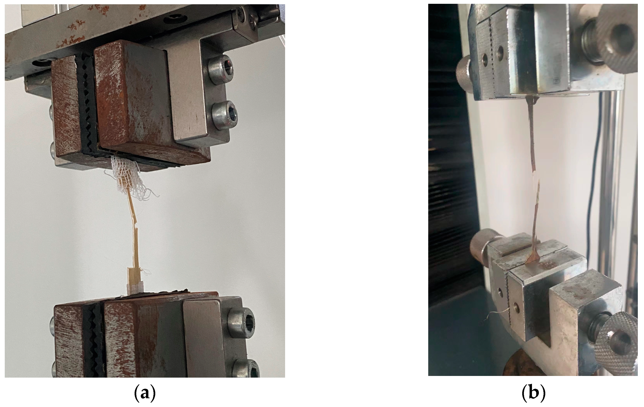
Figure 1.
Tensile test to determine the modulus of elasticity: (a) xylem tensile test; (b) phloem tensile test.
Figure 1.
Tensile test to determine the modulus of elasticity: (a) xylem tensile test; (b) phloem tensile test.
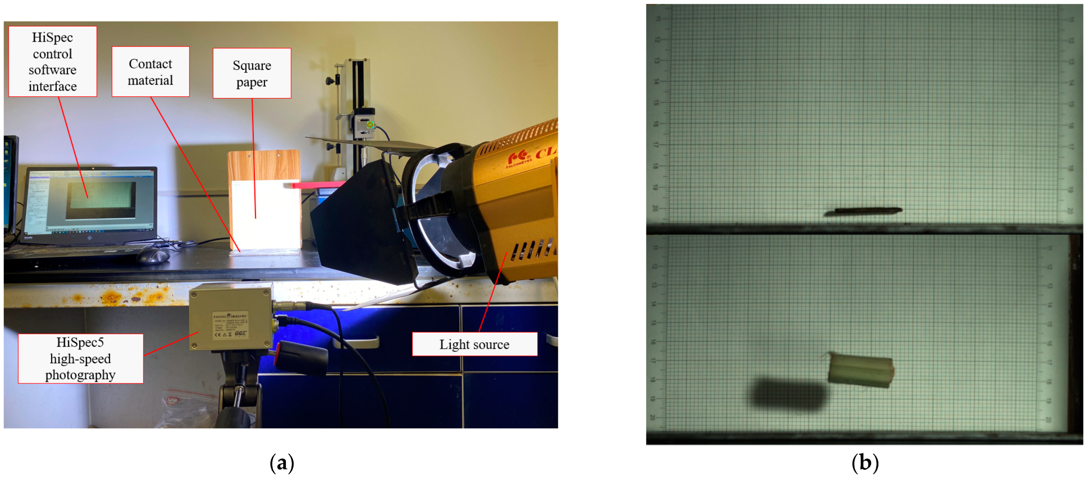
Figure 2.
Measurement of the restitution coefficient: (a) test equipment; (b) keyframe of the rebound’s highest point.
Figure 2.
Measurement of the restitution coefficient: (a) test equipment; (b) keyframe of the rebound’s highest point.
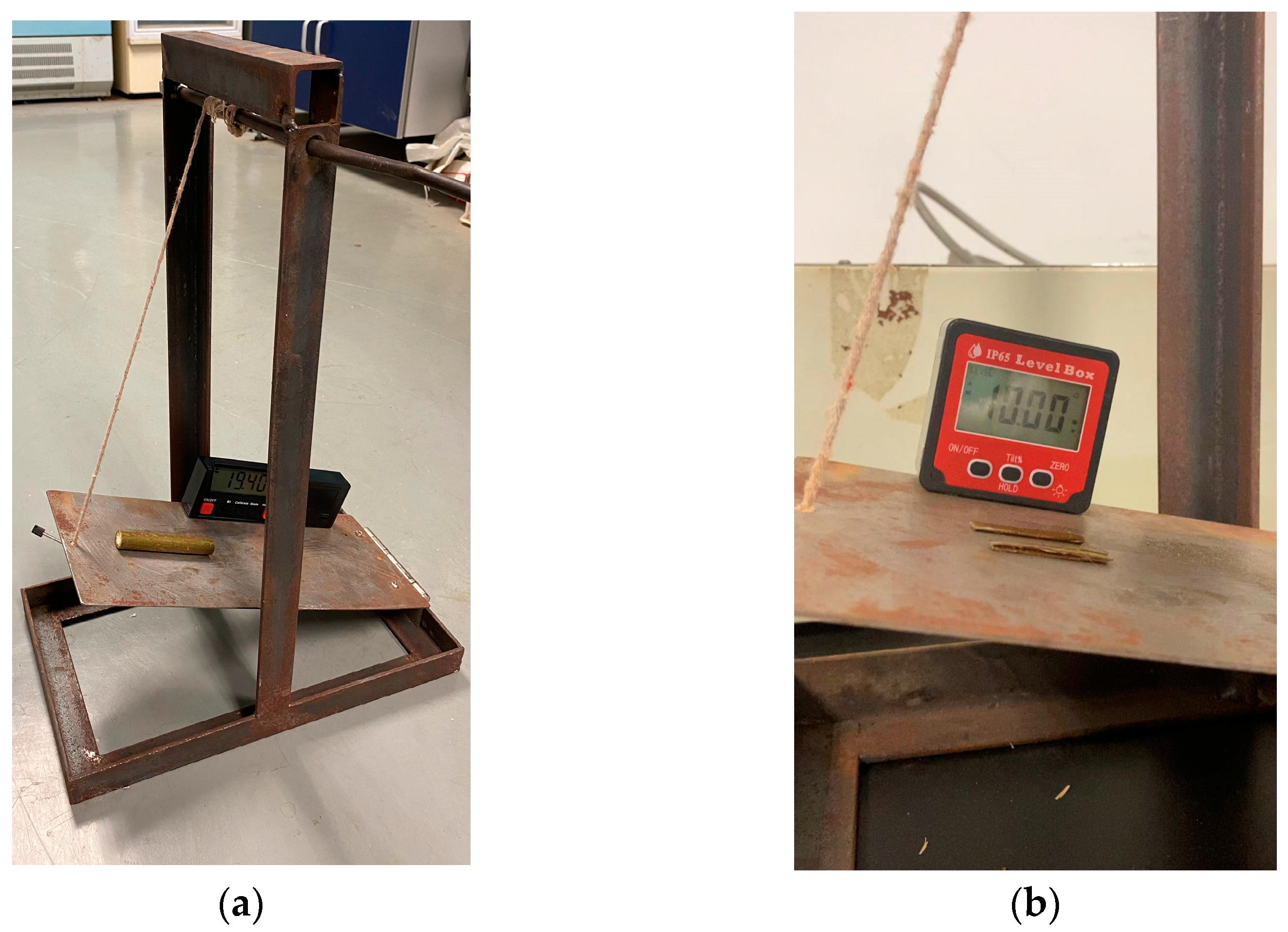
Figure 3.
Measurement of the static friction coefficient: (a) test equipment; (b) sliding angle.
Figure 3.
Measurement of the static friction coefficient: (a) test equipment; (b) sliding angle.
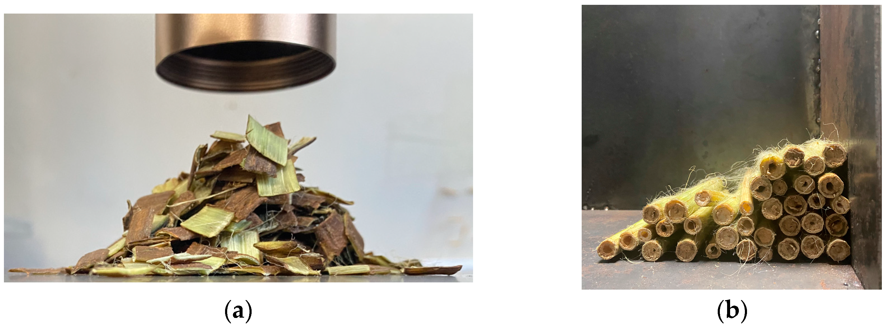
Figure 4.
Physical test of the stacking angle: (a) stacking angle of the phloem; (b) stacking angle of the xylem.
Figure 4.
Physical test of the stacking angle: (a) stacking angle of the phloem; (b) stacking angle of the xylem.
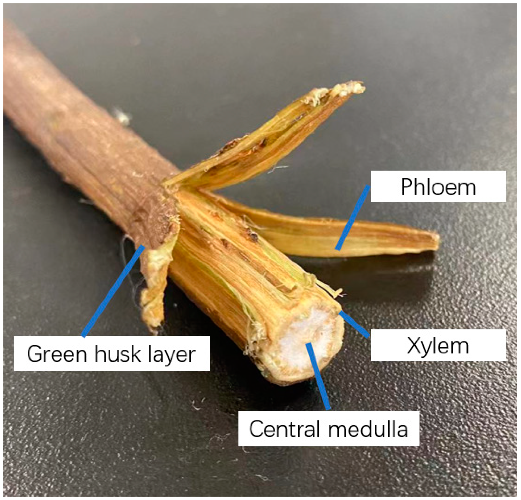
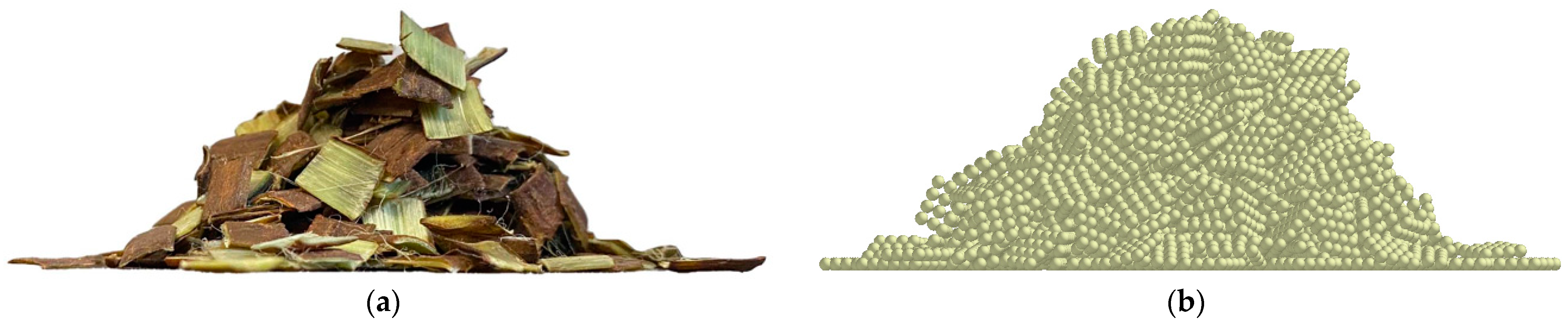
Figure 5.
Schematic diagram of the structural composition of the ramie stalks.
Figure 5.
Schematic diagram of the structural composition of the ramie stalks.
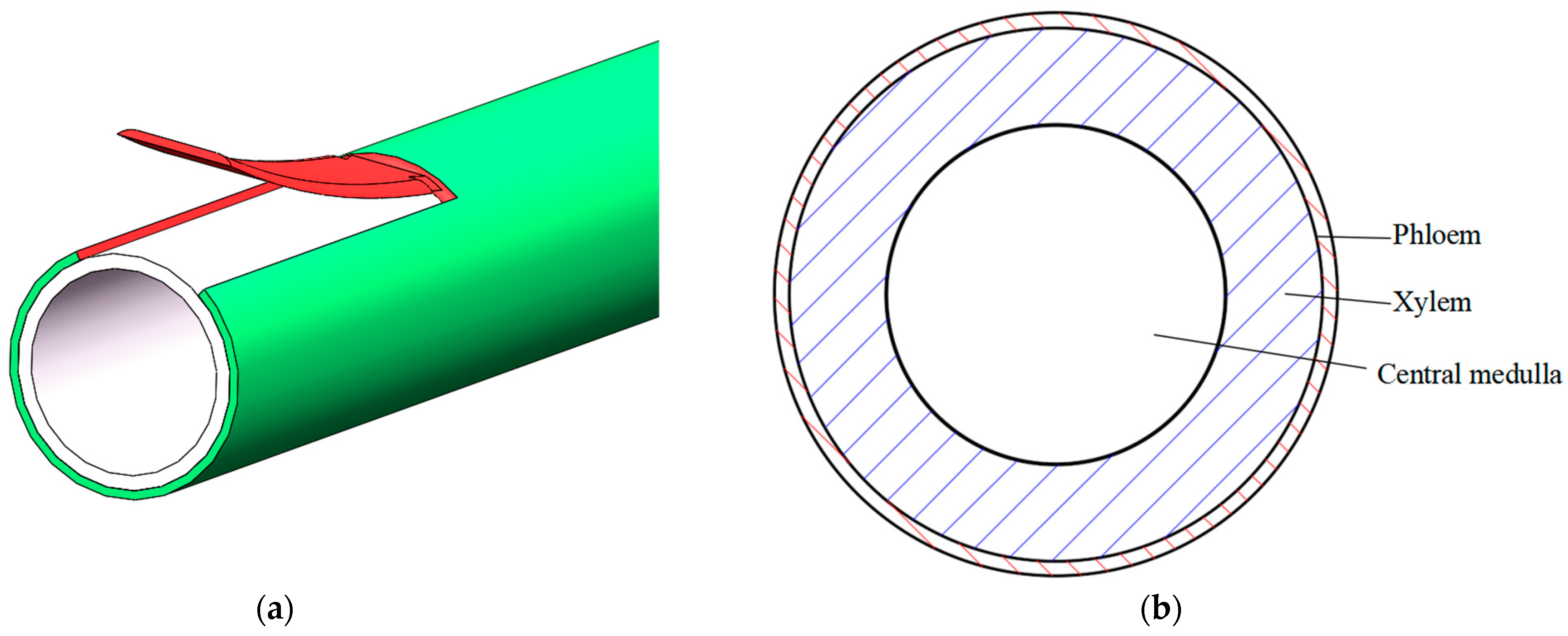
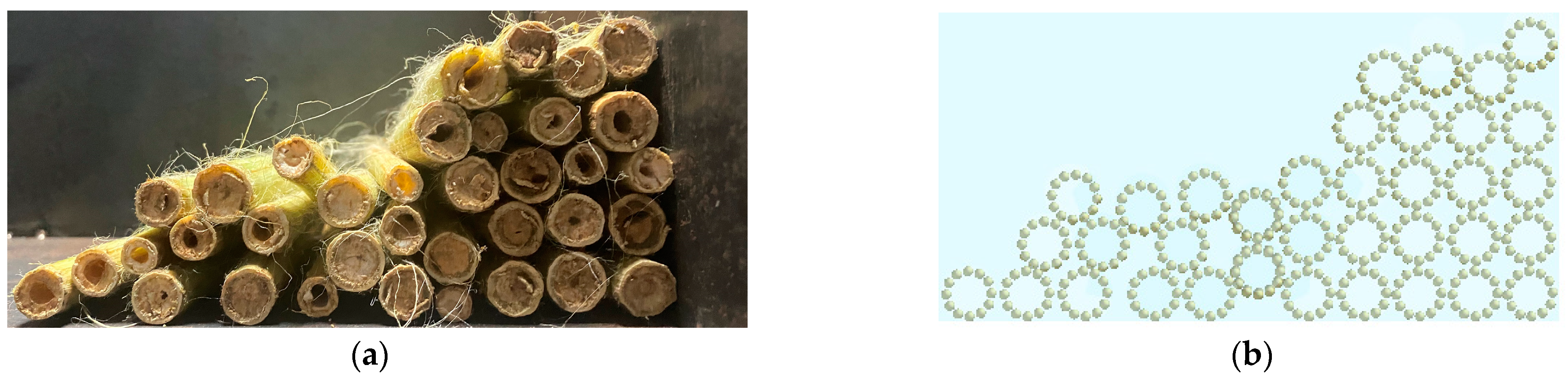
Figure 6.
Ramie stalk geometry model: (a) ramie stalk structure simulation; (b) idealized cross-section of the ramie stalk.
Figure 6.
Ramie stalk geometry model: (a) ramie stalk structure simulation; (b) idealized cross-section of the ramie stalk.
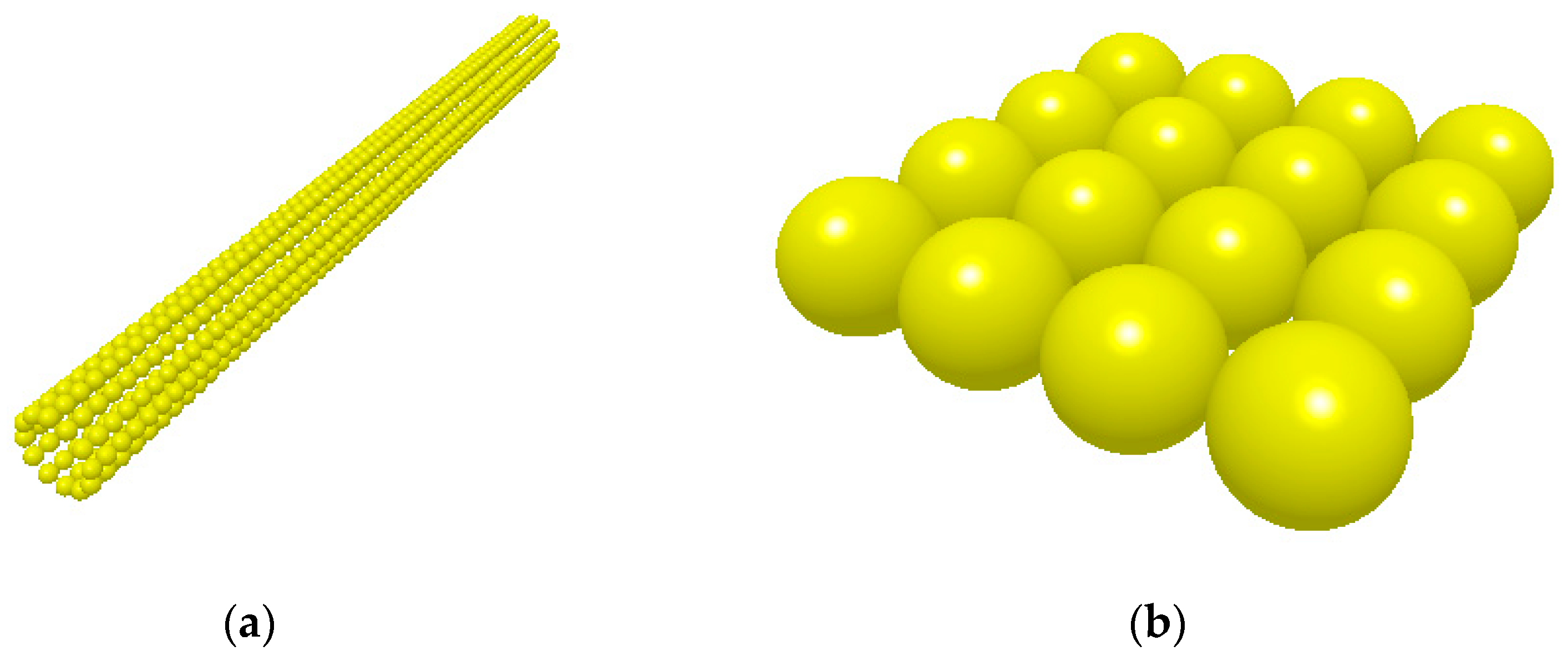
Figure 7.
Ramie stalk discrete element model: (a) xylem discrete element model; (b) phloem discrete element model.
Figure 7.
Ramie stalk discrete element model: (a) xylem discrete element model; (b) phloem discrete element model.
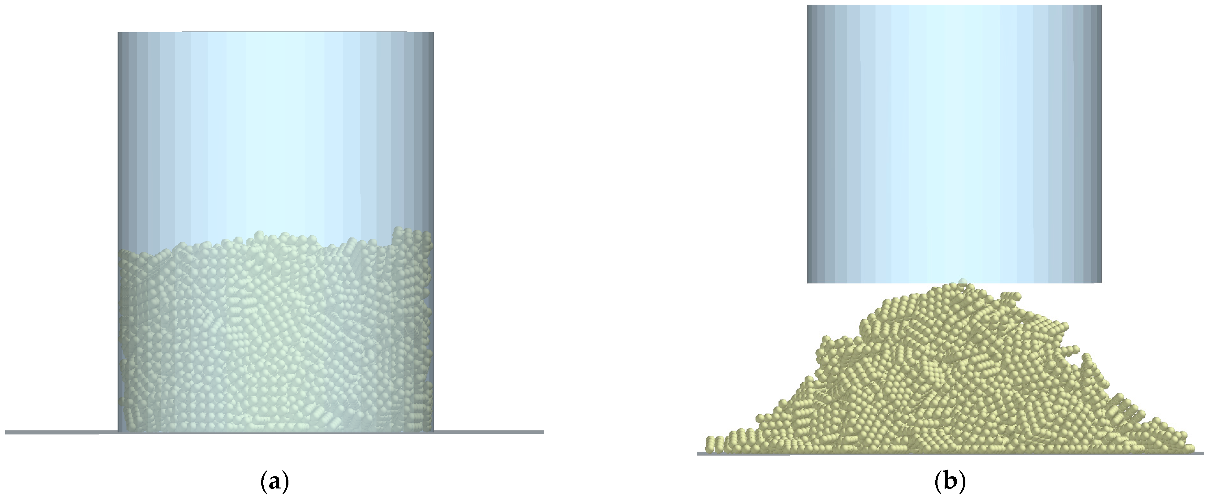
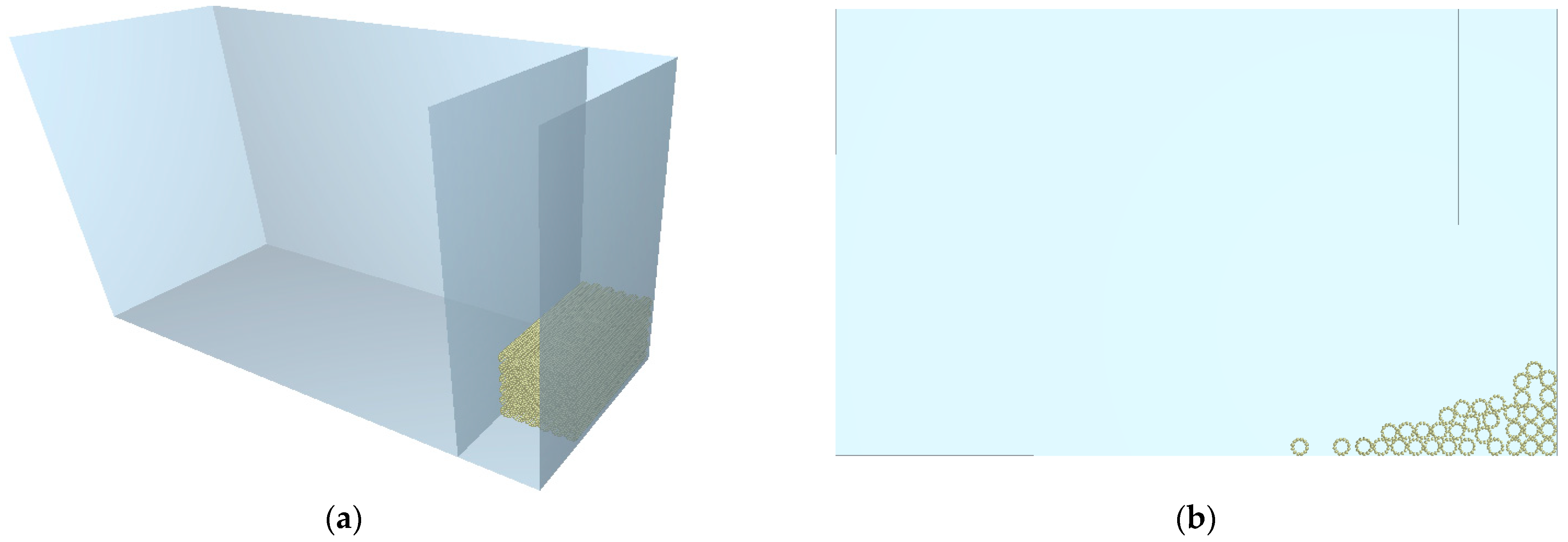
Figure 8.
Ramie phloem stacking angle discrete element simulation test: (a) before stacking; (b) after stacking.
Figure 8.
Ramie phloem stacking angle discrete element simulation test: (a) before stacking; (b) after stacking.
Figure 9.
Ramie xylem stacking angle discrete element simulation test: (a) before stacking; (b) after stacking.
Figure 9.
Ramie xylem stacking angle discrete element simulation test: (a) before stacking; (b) after stacking.
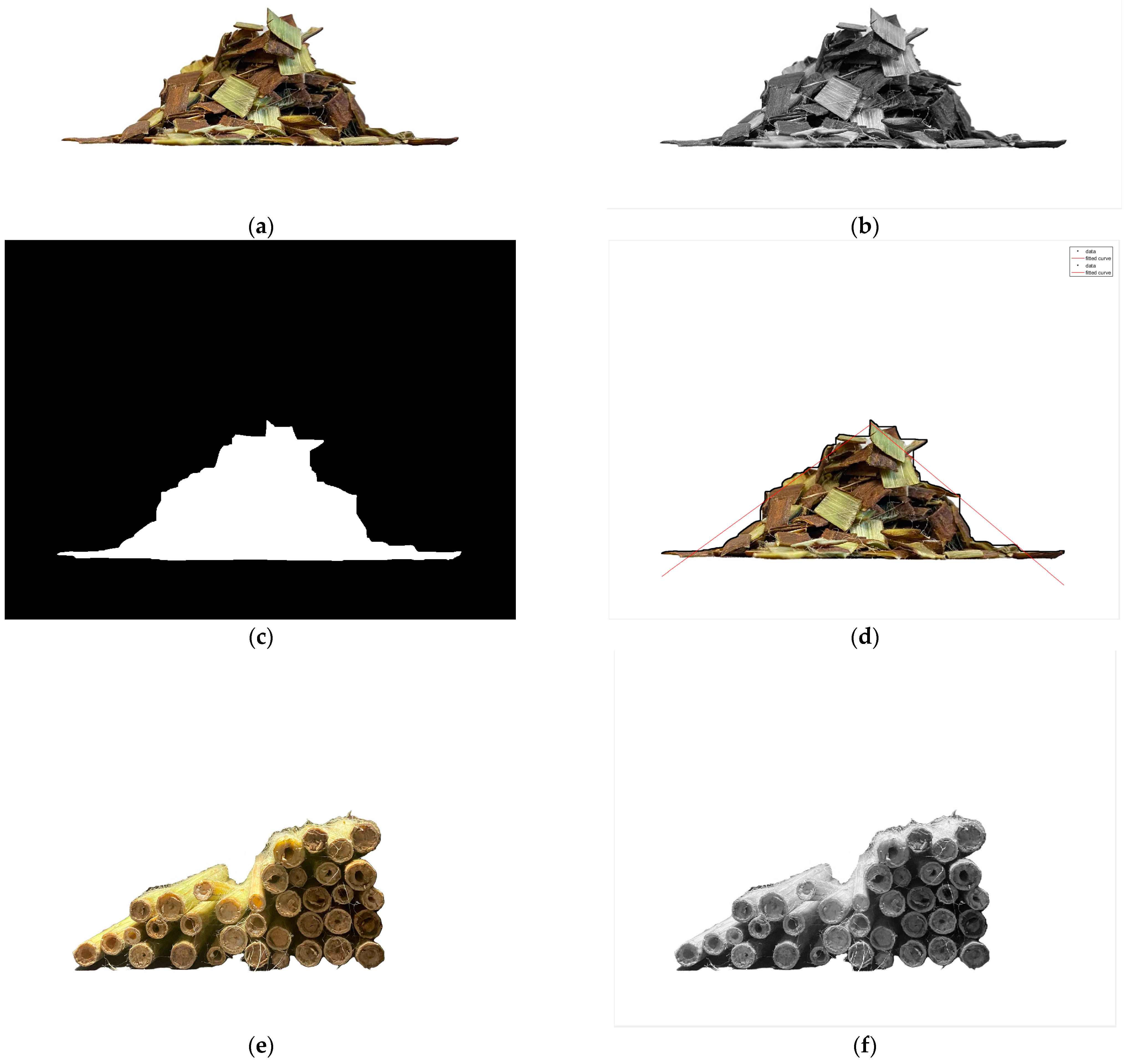
Figure 10.
Physical stacking angle image processing: (a) original image of the phloem stacking angle; (b) grayscale processing of the phloem image; (c) binarization of the phloem image; (d) fitting phloem image using the least squares method; (e) original image of the xylem stacking angle; (f) grayscale processing of the xylem image; (g) binarization of the xylem image; (h) fitting xylem image using the least squares method.
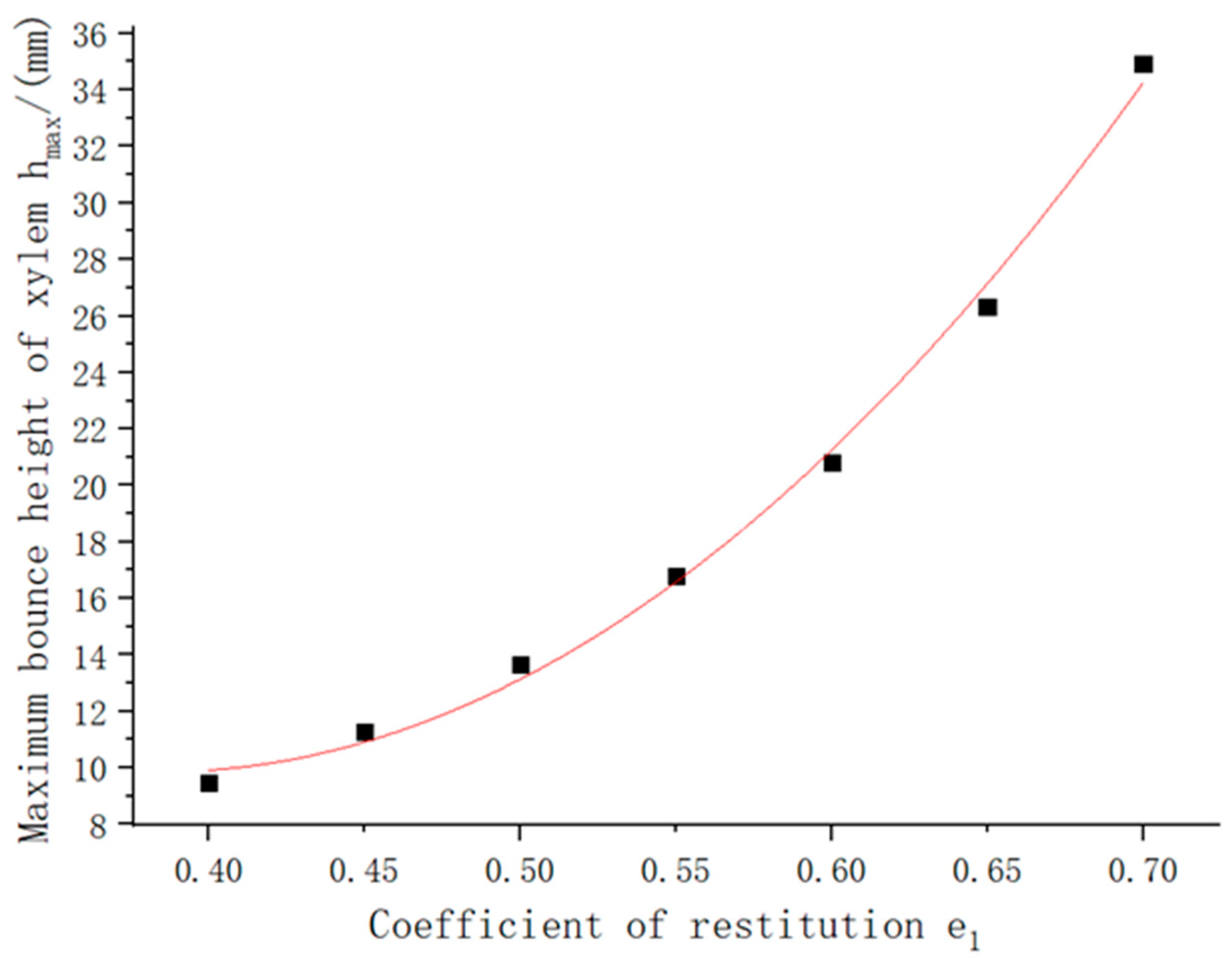
Figure 11.
Fitted curve of the restitution coefficient and maximum rebound height.
Figure 11.
Fitted curve of the restitution coefficient and maximum rebound height.
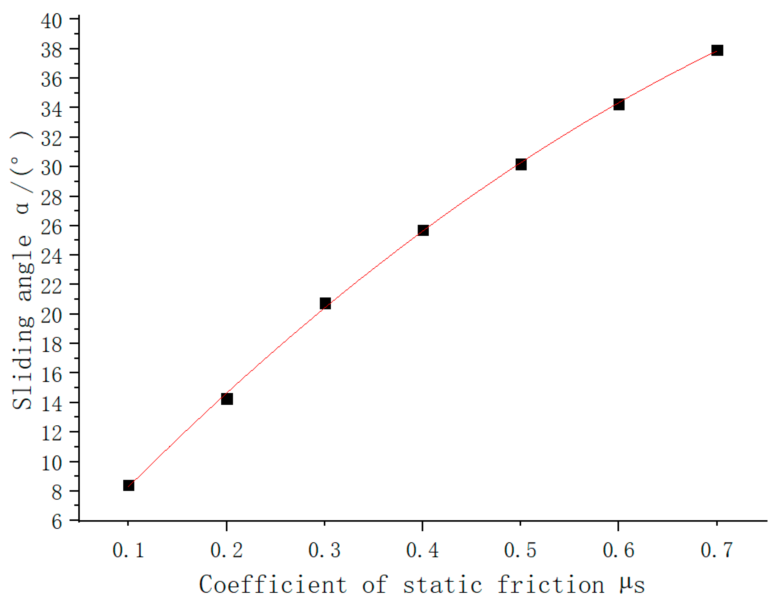
Figure 12.
Fitting curve of the static friction coefficient and sliding angle.
Figure 12.
Fitting curve of the static friction coefficient and sliding angle.
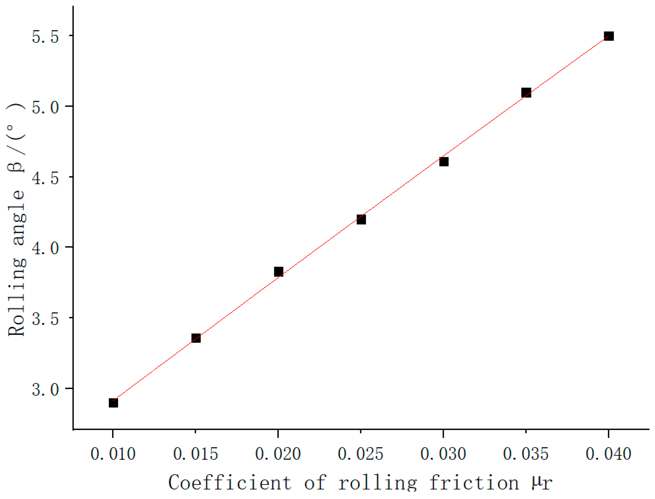
Figure 13.
Fitting curve for the rolling friction coefficient and rolling angle.
Figure 13.
Fitting curve for the rolling friction coefficient and rolling angle.
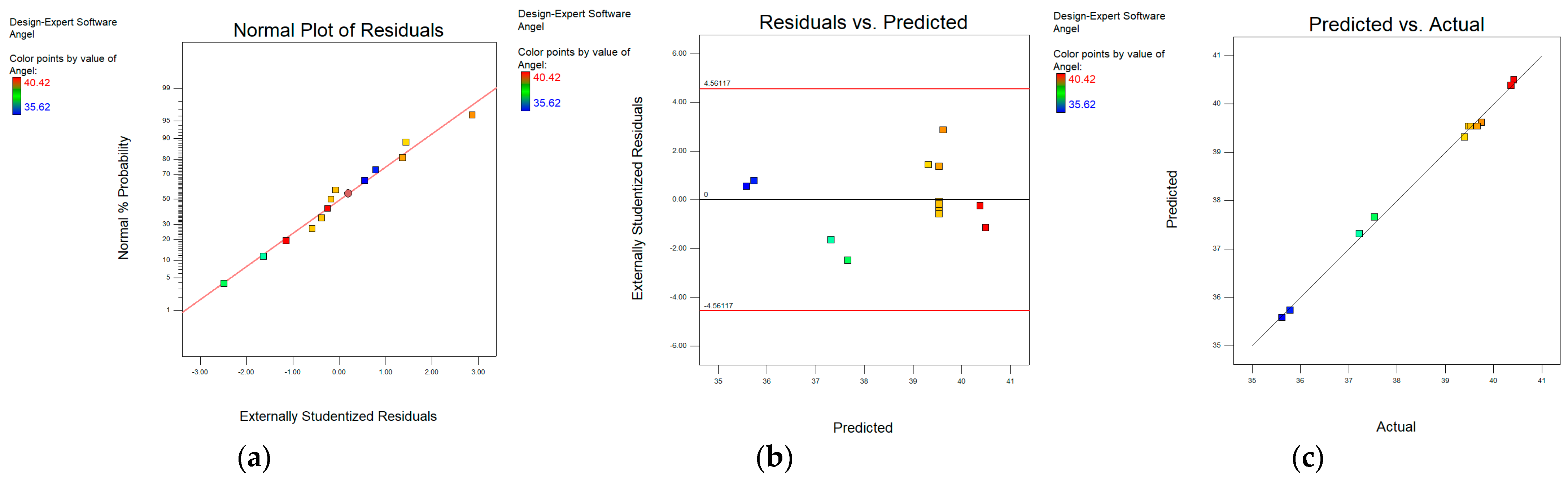
Figure 14.
Diagnostic plot of the phloem quadratic model residuals: (a) normal plot; (b) residual vs. predicted; (c) predicted vs. actual.
Figure 14.
Diagnostic plot of the phloem quadratic model residuals: (a) normal plot; (b) residual vs. predicted; (c) predicted vs. actual.
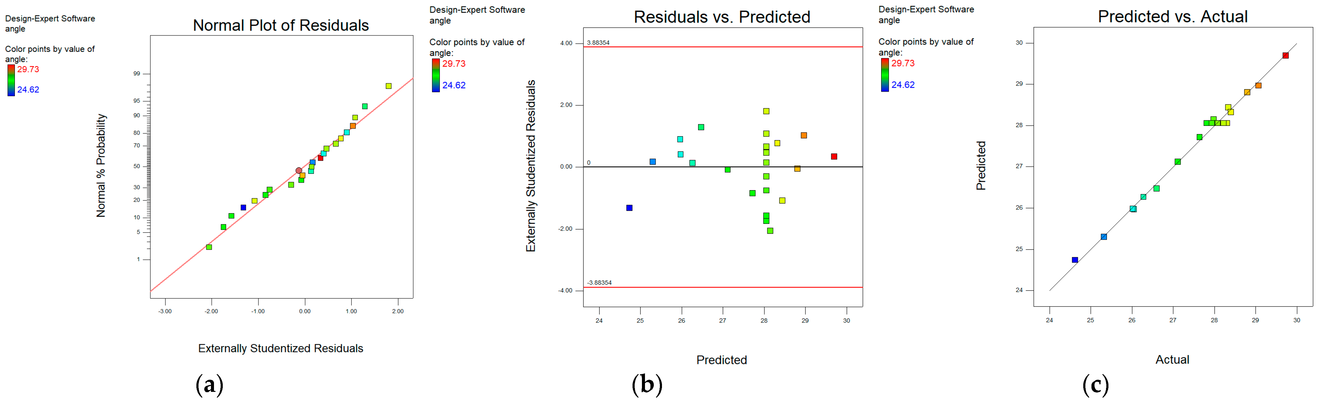
Figure 15.
Diagnostic plot of the xylem quadratic model residuals: (a) normal plot; (b) residual vs. predicted; (c) predicted vs. actual.
Figure 15.
Diagnostic plot of the xylem quadratic model residuals: (a) normal plot; (b) residual vs. predicted; (c) predicted vs. actual.
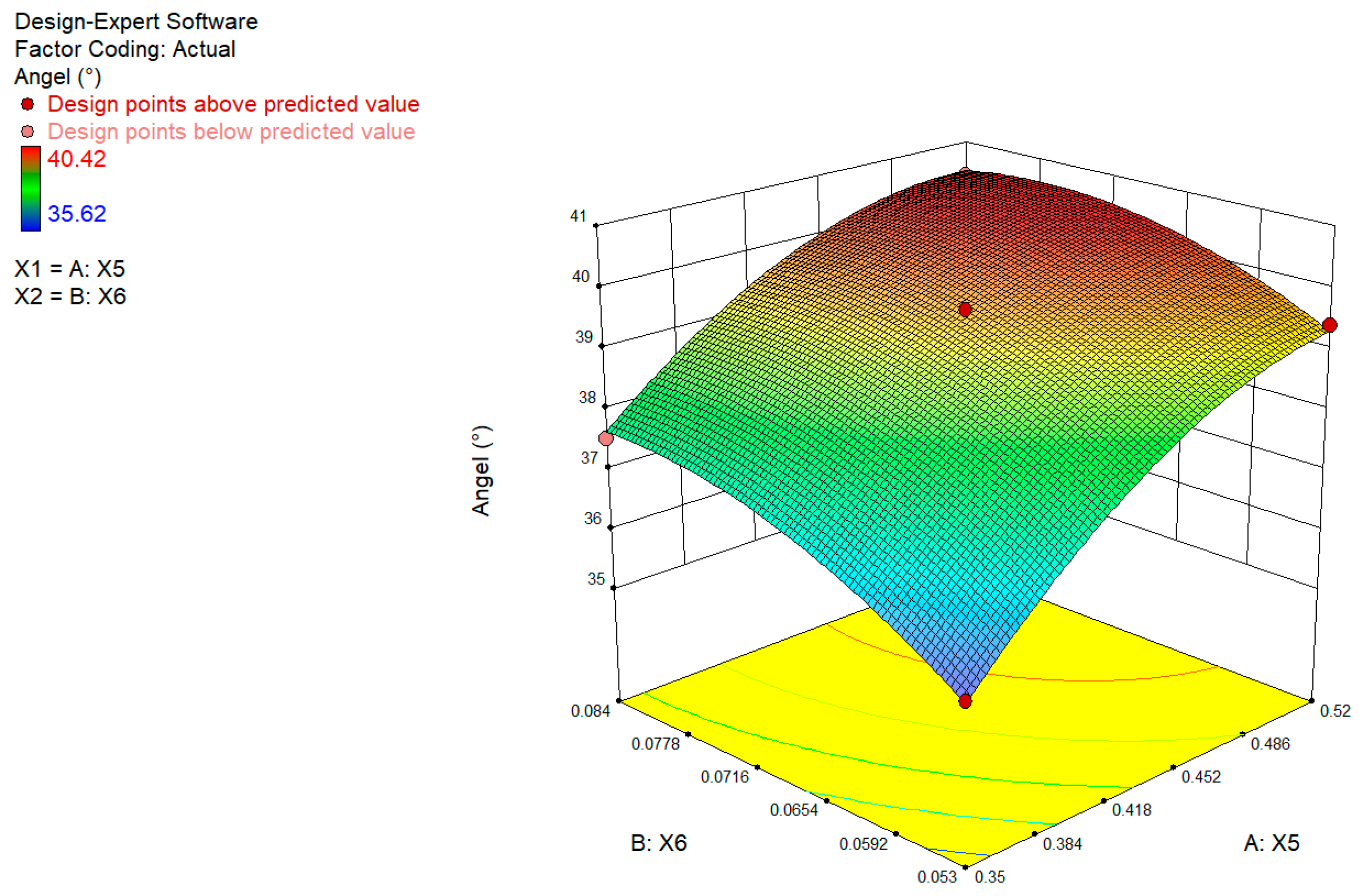
Figure 16.
Response surface of the interaction effects of the factors in the phloem on the stacking angle.
Figure 16.
Response surface of the interaction effects of the factors in the phloem on the stacking angle.
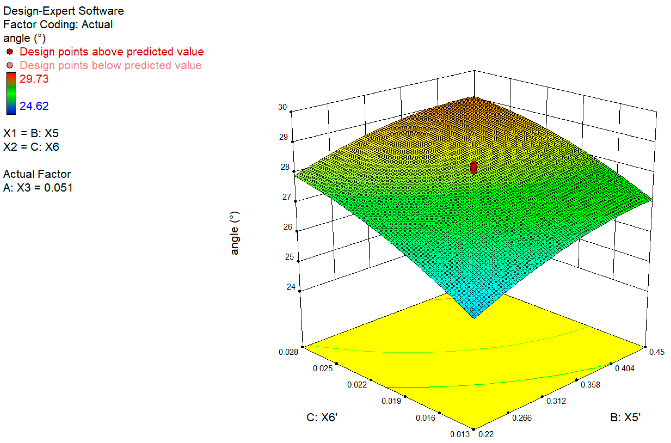
Figure 17.
Response surface of the interaction effects of the factors in the xylem on the stacking angle.
Figure 17.
Response surface of the interaction effects of the factors in the xylem on the stacking angle.
Figure 18.
Comparison of the physical test and simulation test of the ramie phloem stacking angle: (a) physical test; (b) simulation test.
Figure 18.
Comparison of the physical test and simulation test of the ramie phloem stacking angle: (a) physical test; (b) simulation test.
Figure 19.
Comparison of the physical test and simulation test of the ramie xylem stacking angle: (a) physical test; (b) simulation test.
Figure 19.
Comparison of the physical test and simulation test of the ramie xylem stacking angle: (a) physical test; (b) simulation test.
Table 1.
Structural dimensions of the ramie.
Table 1.
Structural dimensions of the ramie.
| Parameters | Max/mm | Min/mm | Mean/mm | Standard Deviation/mm | Variance/mm |
|---|
| Plant height | 2307.00 | 1457.00 | 1969.38 | 217.27 | 4.77 × 10⁴ |
| Xylem outer diameter | 16.11 | 9.00 | 12.56 | 1.58 | 2.51 |
| Xylem inner diameter | 13.07 | 5.31 | 7.98 | 1.26 | 1.60 |
| Phloem thickness | 1.21 | 0.45 | 0.71 | 0.15 | 0.02 |
Table 2.
Plackett–Burman test program.
Table 2.
Plackett–Burman test program.
| Phloem | Xylem |
|---|
| Parameters | Symbols | Levels | Parameters | Symbols | Levels |
| Low level(−1) | High level(+1) | Low level(−1) | High level(+1) |
| Pholem–Q235A steel coefficient of restitution | X1 | 0.05 | 0.45 | Xylem–Q235A steel coefficient of restitution | | 0.17 | 0.57 |
| Pholem–Q235A steel coefficient of static friction | X2 | 0.27 | 0.67 | Xylem–Q235A steel coefficient of static friction | | 0.36 | 0.76 |
| Pholem–Q235A steel coefficient of rolling friction | X3 | 0.005 | 0.100 | Xylem–Q235A steel coefficient of rolling friction | | 0.005 | 0.143 |
| Pholem–Pholem coefficient of restitution | X4 | 0.10 | 0.80 | Xylem–Xylem coefficient of restitution | | 0.10 | 0.80 |
| Pholem–Pholem coefficient of static friction | X5 | 0.10 | 0.60 | Xylem–Xylem coefficient of static friction | | 0.10 | 0.80 |
| Pholem–Pholem coefficient of rolling friction | X6 | 0.005 | 0.100 | Xylem–Xylem coefficient of rolling friction | | 0.005 | 0.050 |
Table 3.
Parameters required for the discrete element simulation.
Table 3.
Parameters required for the discrete element simulation.
| Parameter Type | DEM Parameter | Parameter Value | Source |
|---|
| Physical Parameters | Density of Q235A steel (kg/m3) | 7850 | Literature [47] |
| Shear modulus of Q235A steel (Pa) | 7.90 × 10¹⁰ | Literature [47] |
| Poisson’s ratio of Q235A steel | 0.30 | Literature [47] |
| Density of phloem (kg/m3) | 202.37 | Section 2.1.2 |
| Shear modulus of phloem (Pa) | 6.15 × 10⁸ | Section 2.1.3 |
| Poisson’s ratio of phloem | 0.40 | Literature [48] |
| Density of xylem (kg/m3) | 751.50 | Section 2.1.2 |
| Shear modulus of xylem (Pa) | 2.42 × 10⁸ | Section 2.1.3 |
| Poisson’s ratio of xylem | 0.30 | Literature [48] |
| Contact Parameters | Phloem–Q235A steel coefficient of restitution | 0.25 | Section 2.2.1 |
| Phloem–Q235A steel coefficient of static friction | 0.47 | Section 2.2.2 |
| Phloem–Q235A steel coefficient of rolling friction | 0.05 | Section 2.2.2 |
| Xylem–Q235A steel coefficient of restitution | 0.37 | Section 2.2.1 |
| Xylem–Q235A steel coefficient of static friction | 0.56 | Section 2.2.2 |
| Xylem–Q235A steel coefficient of restitution | 0.074 | Section 2.2.2 |
Table 4.
Simulation test results for the restitution coefficient between xylem and phloem.
Table 4.
Simulation test results for the restitution coefficient between xylem and phloem.
| No. | Coefficient of Restitution, e1 | Maximum Bounce Height of Xylem, hmax/mm |
|---|
| 1 | 0.40 | 9.46 |
| 2 | 0.45 | 11.26 |
| 3 | 0.50 | 13.67 |
| 4 | 0.55 | 16.78 |
| 5 | 0.60 | 20.80 |
| 6 | 0.65 | 26.32 |
| 7 | 0.7 | 34.91 |
Table 5.
Simulation test results for the static friction coefficient between the xylem and phloem.
Table 5.
Simulation test results for the static friction coefficient between the xylem and phloem.
| No. | Coefficient of Static Friction, µs | Sliding Angle, α (°) |
|---|
| 1 | 0.10 | 8.43 |
| 2 | 0.20 | 14.28 |
| 3 | 0.30 | 20.75 |
| 4 | 0.40 | 25.72 |
| 5 | 0.50 | 30.19 |
| 6 | 0.60 | 34.26 |
| 7 | 0.70 | 37.93 |
Table 6.
Simulation test results for the rolling friction coefficient between the xylem and phloem.
Table 6.
Simulation test results for the rolling friction coefficient between the xylem and phloem.
| No. | Coefficient of Rolling Friction, µr | Rolling Angle, β (°) |
|---|
| 1 | 0.010 | 2.90 |
| 2 | 0.015 | 3.36 |
| 3 | 0.020 | 3.83 |
| 4 | 0.025 | 4.20 |
| 5 | 0.030 | 4.61 |
| 6 | 0.035 | 5.10 |
| 7 | 0.040 | 5.50 |
Table 7.
Phloem Plackett–Burman test results.
Table 7.
Phloem Plackett–Burman test results.
| X1 | X2 | X3 | X4 | X5 | X6 | Angle (°) |
|---|
| −1 | −1 | −1 | −1 | −1 | −1 | 18.19 |
| −1 | 1 | 1 | −1 | 1 | −1 | 38.94 |
| 1 | −1 | 1 | −1 | −1 | −1 | 19.40 |
| −1 | 1 | −1 | −1 | −1 | 1 | 30.67 |
| 0 | 0 | 0 | 0 | 0 | 0 | 36.35 |
| 1 | 1 | −1 | 1 | −1 | −1 | 20.19 |
| 1 | 1 | 1 | −1 | 1 | 1 | 42.99 |
| 1 | −1 | 1 | 1 | −1 | 1 | 30.03 |
| 1 | 1 | −1 | 1 | 1 | −1 | 39.12 |
| −1 | −1 | −1 | 1 | 1 | 1 | 41.25 |
| −1 | −1 | 1 | 1 | 1 | −1 | 38.64 |
| −1 | 1 | 1 | 1 | −1 | 1 | 31.28 |
| 1 | −1 | −1 | −1 | 1 | 1 | 41.59 |
Table 8.
Parameter significance analysis of the Plackett–Burman test in the phloem.
Table 8.
Parameter significance analysis of the Plackett–Burman test in the phloem.
| Parameters | Degree of Freedom | Sum of Squares | F-Value | p-Value | Effect Value | Significance Ranking |
|---|
| X1 | 1 | 2.67 | 0.59 | 0.5239 | −0.94 | 6 |
| X2 | 1 | 16.52 | 3.65 | 0.1433 | 2.35 | 3 |
| X3 | 1 | 8.82 | 1.95 | 0.2647 | 1.71 | 4 |
| X4 | 1 | 6.35 | 1.40 | 0.3370 | 1.45 | 5 |
| X5 | 1 | 717.30 | 158.39 | <0.0001 | 15.46 | 1 |
| X6 | 1 | 156.46 | 34.55 | 0.0021 | 7.22 | 2 |
Table 9.
Xylem Plackett–Burman test results.
Table 9.
Xylem Plackett–Burman test results.
| | | | | | Angle (°) |
|---|
| 1 | 1 | 1 | −1 | 1 | 1 | 38.61 |
| 1 | 1 | −1 | 1 | 1 | −1 | 27.52 |
| 1 | −1 | 1 | −1 | −1 | −1 | 27.33 |
| −1 | 1 | 1 | −1 | 1 | −1 | 31.96 |
| −1 | −1 | −1 | 1 | 1 | 1 | 33.84 |
| −1 | −1 | 1 | 1 | 1 | −1 | 32.07 |
| 1 | 1 | −1 | 1 | −1 | −1 | 22.26 |
| −1 | 1 | 1 | 1 | −1 | 1 | 34.02 |
| 0 | 0 | 0 | 0 | 0 | 0 | 31.10 |
| 1 | −1 | −1 | −1 | 1 | 1 | 33.71 |
| −1 | 1 | −1 | −1 | −1 | 1 | 30.55 |
| −1 | −1 | −1 | −1 | −1 | −1 | 19.65 |
| 1 | −1 | 1 | 1 | −1 | 1 | 34.91 |
Table 10.
Parameter significance analysis of the Plackett–Burman test in the xylem.
Table 10.
Parameter significance analysis of the Plackett–Burman test in the xylem.
| Parameters | Degree of Freedom | Sum of Squares | F-Value | p-Value | Effect Value | Significance Ranking |
|---|
| X1 | 1 | 0.43 | 0.33 | 0.5620 | 0.38 | 6 |
| X2 | 1 | 0.97 | 0.75 | 0.3900 | 0.57 | 4 |
| X3 | 1 | 82.05 | 63.22 | 0.0001 | 5.23 | 2 |
| X4 | 1 | 0.66 | 0.51 | 0.4741 | 0.47 | 5 |
| X5 | 1 | 70.05 | 53.98 | 0.0002 | 4.83 | 3 |
| X6 | 1 | 167.58 | 129.14 | <0.0001 | 7.47 | 1 |
Table 11.
Results of the steepest ascent test of the phloem.
Table 11.
Results of the steepest ascent test of the phloem.
| No. | X5 | X6 | Stacking Angle (°) | Relative Error (%) |
|---|
| 1 | 0.10 | 0.005 | 19.50 | 50.43 |
| 2 | 0.18 | 0.021 | 25.49 | 35.21 |
| 3 | 0.27 | 0.037 | 31.35 | 20.31 |
| 4 | 0.35 | 0.053 | 35.56 | 9.62 |
| 5 | 0.43 | 0.068 | 39.57 | 0.58 |
| 6 | 0.52 | 0.084 | 40.45 | 2.82 |
| 7 | 0.60 | 0.100 | 43.13 | 9.61 |
Table 12.
Results of the steepest ascent test of the xylem.
Table 12.
Results of the steepest ascent test of the xylem.
| No. | X3′ | X5′ | X6′ | Stacking Angle (°) | Relative Error (%) |
|---|
| 1 | 0.005 | 0.10 | 0.005 | 16.50 | 39.27 |
| 2 | 0.028 | 0.22 | 0.013 | 24.60 | 9.45 |
| 3 | 0.051 | 0.33 | 0.020 | 28.22 | 3.87 |
| 4 | 0.074 | 0.45 | 0.028 | 29.72 | 9.40 |
| 5 | 0.097 | 0.57 | 0.035 | 32.41 | 19.30 |
| 6 | 0.120 | 0.68 | 0.043 | 32.90 | 21.08 |
| 7 | 0.143 | 0.80 | 0.050 | 33.13 | 21.93 |
Table 13.
Factor level codes for the phloem central composite design test.
Table 13.
Factor level codes for the phloem central composite design test.
| Coding | Phloem–Phloem Coefficient of Static Friction X5 | Phloem–Phloem Coefficient of Rolling Friction X6 |
|---|
| −1.414 | 0.31 | 0.047 |
| −1 | 0.35 | 0.053 |
| 0 | 0.43 | 0.068 |
| 1 | 0.52 | 0.084 |
| 1.414 | 0.56 | 0.090 |
Table 14.
The phloem central composite design test scheme and results.
Table 14.
The phloem central composite design test scheme and results.
| No. | X5 | X6 | Stacking Angle Y1 (°) |
|---|
| 1 | −1.414 | 0 | 35.82 |
| 2 | −1 | −1 | 35.65 |
| 3 | −1 | 1 | 37.57 |
| 4 | 0 | −1.414 | 37.25 |
| 5 | 0 | 0 | 39.69 |
| 6 | 0 | 0 | 39.53 |
| 7 | 0 | 0 | 39.51 |
| 8 | 0 | 0 | 39.56 |
| 9 | 0 | 0 | 39.55 |
| 10 | 0 | 1.414 | 39.78 |
| 11 | 1 | −1 | 39.43 |
| 12 | 1 | 1 | 40.45 |
| 13 | 1.414 | 0 | 40.39 |
Table 15.
ANOVA results of the phloem stacking angle.
Table 15.
ANOVA results of the phloem stacking angle.
| Source | Stacking Angle Y1 (°) |
|---|
| Sum of Squares | df | Mean Square | F-Value | p-Value |
|---|
| Model | 32.21 | 5 | 6.44 | 576.29 | <0.0001 ** |
| X5 | 21.53 | 1 | 21.53 | 1925.51 | <0.0001 ** |
| X6 | 5.31 | 1 | 5.31 | 475.01 | <0.0001 ** |
| X5X6 | 0.20 | 1 | 0.20 | 18.11 | 0.0038 ** |
| 3.81 | 1 | 3.81 | 340.97 | <0.0001 ** |
| 1.99 | 1 | 1.99 | 178.27 | <0.0001 ** |
| Residual | 0.078 | 7 | 0.011 | | |
| Lack of Fit | 0.058 | 3 | 0.019 | 3.86 | 0.1123 |
| Pure Error | 0.020 | 4 | 5.020 × 10⁻³ | | |
| Cor Total | 32.29 | 12 | | | |
Table 16.
Factor level codes for the xylem central composite design test.
Table 16.
Factor level codes for the xylem central composite design test.
| Coding | Xylem–Q235A Steel Coefficient of Rolling Friction X3′ | Xylem–Xylem Coefficient of Static Friction X5′ | Xylem–Xylem Coefficient of Rolling Friction X6′ |
|---|
| −1.682 | 0.012 | 0.14 | 0.007 |
| −1 | 0.028 | 0.22 | 0.013 |
| 0 | 0.051 | 0.33 | 0.020 |
| 1 | 0.074 | 0.45 | 0.028 |
| 1.682 | 0.090 | 0.53 | 0.033 |
Table 17.
The xylem central composite design test scheme and results.
Table 17.
The xylem central composite design test scheme and results.
| No. | X3 | X5 | X6 | Stacking Angle Y2 (°) |
|---|
| 1 | 1 | 0 | 0 | 28.01 |
| 2 | 1 | 1 | −1 | 27.64 |
| 3 | 1 | 1 | 1 | 29.73 |
| 4 | 0 | 0 | 0 | 27.83 |
| 5 | −1 | −1 | 1 | 27.11 |
| 6 | 0 | 0 | 0 | 27.81 |
| 7 | 1 | −1 | 1 | 28.34 |
| 8 | 0 | 0 | 0 | 28.22 |
| 9 | 0 | 0 | 0 | 28.08 |
| 10 | 0 | 0 | 0 | 28.13 |
| 11 | −1 | 1 | 1 | 27.98 |
| 12 | 1 | −1 | −1 | 26.05 |
| 13 | −1.682 | 0 | 0 | 26.60 |
| 14 | 1.682 | 0 | 0 | 28.80 |
| 15 | 0 | 0 | 0 | 27.94 |
| 16 | 0 | 0 | −1.682 | 25.32 |
| 17 | −1 | 1 | −1 | 26.28 |
| 18 | 0 | 1.682 | 0 | 28.40 |
| 19 | 0 | 0 | 0 | 28.16 |
| 20 | 0 | 0 | 1.682 | 29.07 |
| 21 | 0 | 0 | 0 | 28.31 |
| 22 | 0 | −1.682 | 0 | 26.02 |
| 23 | −1 | −1 | −1 | 24.62 |
Table 18.
ANOVA results of the xylem stacking angle.
Table 18.
ANOVA results of the xylem stacking angle.
| Source | Stacking Angle Y2 (°) |
|---|
| Sum of Squares | df | Mean Square | F-Value | p-Value |
|---|
| Model | 33.18 | 9 | 3.69 | 141.54 | <0.0001 ** |
| X3 | 6.57 | 1 | 6.57 | 252.10 | <0.0001 ** |
| X5 | 6.63 | 1 | 6.63 | 254.38 | <0.0001 ** |
| X6 | 16.21 | 1 | 16.21 | 622.14 | <0.0001 ** |
| X3X5 | 0.025 | 1 | 0.025 | 0.97 | 0.3422 |
| X3X6 | 4.512 × 10⁻³ | 1 | 4.512 × 10⁻³ | 0.17 | 0.6840 |
| X5X6 | 0.12 | 1 | 0.12 | 4.70 | 0.0492 * |
| 0.35 | 1 | 0.35 | 13.34 | 0.0029 ** |
| 1.64 | 1 | 1.64 | 62.83 | <0.0001 ** |
| 1.69 | 1 | 1.69 | 64.93 | <0.0001 ** |
| Residual | 0.34 | 13 | 0.026 | | |
| Lack of Fit | 0.10 | 5 | 0.021 | 0.70 | 0.6381 |
| Pure Error | 0.24 | 8 | 0.029 | | |
| Cor Total | 33.52 | 22 | | | |
Table 19.
Results of the phloem F-test.
Table 19.
Results of the phloem F-test.
| | Mean (°) | Variance | Observed Value | df | F | p (F ≤ f) One-Tailed | F One-Tailed Critical |
|---|
| Simulated value | 38.04 | 0.0219 | 5 | 4 | 0.0041 | 5.1495 × 10⁻⁵ | 0.1565 |
| Physical value | 37.93 | 5.2639 | 5 | 4 | | | |
Table 20.
Results of the phloem two-sample heteroskedasticity t-test.
Table 20.
Results of the phloem two-sample heteroskedasticity t-test.
| | Mean (°) | Variance | Observed Value | Assume Average Difference | df | t Stat | p (T ≤ t) One-Tailed | t One-Tailed Critical | p (T ≤ t)
Two-Tailed | t Two-Tailed Critical |
|---|
| Simulated value | 38.04 | 0.02193 | 5 | 0 | 4 | 0.1120 | 0.4581 | 2.1318 | 0.9162 | 2.7764 |
| Physical value | 37.93 | 5.2639 | 5 | | | | | | | |
Table 21.
Results of the xylem F-test.
Table 21.
Results of the xylem F-test.
| | Mean (°) | Variance | Observed Value | df | F | p (F ≤ f) One-Tailed | F One-Tailed Critical |
|---|
| Simulated value | 27.20 | 0.0190 | 5 | 4 | 0.0119 | 0.0004 | 0.1565 |
| Physical value | 27.17 | 1.6004 | 5 | 4 | | | |
Table 22.
Results of the xylem two-sample heteroskedasticity t-test.
Table 22.
Results of the xylem two-sample heteroskedasticity t-test.
| | Mean (°) | Variance | Observed Value | Assume Average Difference | df | t Stat | p (T ≤ t) One-Tailed | t One-Tailed Critical | p (T ≤ t) Two-Tailed | t Two-Tailed Critical |
|---|
| Simulated value | 27.20 | 0.0190 | 5 | 0 | 4 | 0.0459 | 0.4828 | 2.1318 | 0.9656 | 2.7764 |
| Physical value | 27.17 | 1.6004 | 5 | | | | | | | |


