
Agricultural Combine Remaining Value Forecasting Methodology and Model (and Derived Tool)

Abstract
:
1. Introduction
1.1. Previous Studies
1.2. Current Issues
1.3. Goal
2. Materials and Methods
2.1. Dataset
2.2. Data Systematization and Preprocessing
2.2.1. New Equivalent Combine
2.2.2. Combine Family
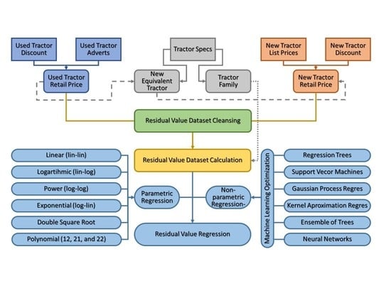
2.3. Data Analysis
3. Results
4. Discussion
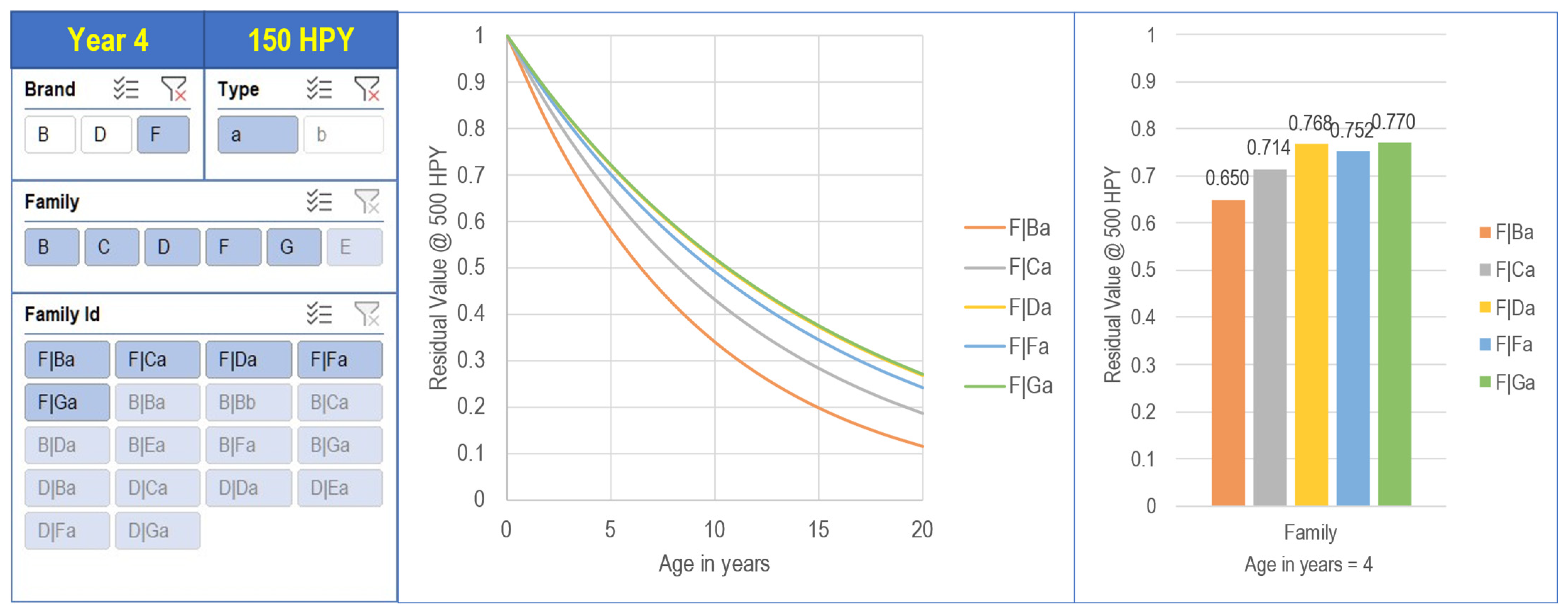
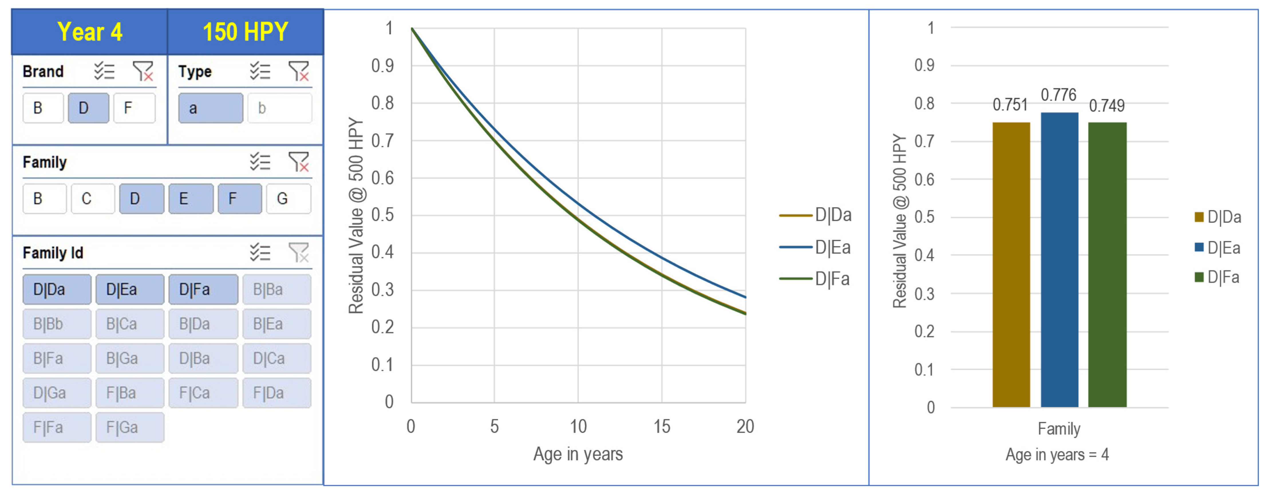
Methodology and Model Derived Grain Combine Harvester Remaining Value Forecaster Tool
5. Conclusions
Author Contributions
Funding
Institutional Review Board Statement
Data Availability Statement
Acknowledgments
Conflicts of Interest
References
- FAO. Handbook on Agricultural Cost of Production Statistics; FAO: Rome, Italy, 2016. [Google Scholar]
- Strivastava, A.K.; Goering, C.E.; Rohrbach, R.P.; Buckmaster, D.R. Machinery Selection and Management. In Engineering Principles of Agricultural Machines; American Society of Agricultural and Biological Engineers: St. Joseph, MI, USA, 2006; Chapter 15; pp. 525–552. [Google Scholar]
- Strivastava, A.K.; Goering, C.E.; Rohrbach, R.P.; Buckmaster, D.R. Grain Harvesting. In Engineering Principles of Agricultural Machines; American Society of Agricultural and Biological Engineers: St. Joseph, MI, USA, 2006; Chapter 12; pp. 403–436. [Google Scholar]
- AXEMA. Economic Report; AXEMA: Paris, France, 2022. [Google Scholar]
- CEMA. European Agricultural Machinery Industry Key Figures; CEMA: Brussels, Belgium, 2022. [Google Scholar]
- Isaac, N.E.; Quick, G.R.; Birrell, S.J.; Edwards, W.M.; Coers, B.A. Combine Harvester Econometric Model with Forward Speed Optimization. Appl. Eng. Agric. 2006, 22, 25–31. [Google Scholar] [CrossRef]
- ACEA. Economic and Market Report. State of the EU Auto Industry. Full-Year 2021; European Automobile Manufacturers’ Association (ACEA): Brussels, Belgium, 2022. [Google Scholar]
- CEMA. Economic Press Release Tractor Registrations 2021; CEMA Aisbl—European Agricultural Machinery: Brussels, Belgium, 2022. [Google Scholar]
- Weersink, A.; Stauber, S. Optimal Replacement Interval and Depreciation Method for a Grain Combine. West. J. Agric. Econ. 1988, 13, 18–28. [Google Scholar]
- Leatham, D.J.; Baker, T.G. Empirical Estimates of the Effects of Inflation on Salvage Values, Cost and Optimal Replacement of Tractors and Combines. North Cent. J. Agric. Econ. 1981, 3, 109–117. [Google Scholar] [CrossRef]
- Cross, T.L.; Perry, G.M. Depreciation Patterns for Agricultural Machinery. Am. J. Agric. Econ. 1995, 77, 194–204. [Google Scholar] [CrossRef]
- Cross, T.L.; Perry, G.M. Remaining Value Functions for Farm Equipment. Appl. Eng. Agric. 1996, 12, 547–553. [Google Scholar] [CrossRef]
- Unterschultz, J.; Mumey, G. Reducing Investment Risk in Tractors and Combines with Improved Terminal Asset Value Forecasts. Can. J. Agric. Econ. 1996, 44, 295–309. [Google Scholar] [CrossRef]
- Wu, J.; Perry, G.M. Estimating Farm Equipment Depreciation: Which Functional Form Is Best? Am. J. Agric. Econ. 2004, 86, 483–491. [Google Scholar] [CrossRef]
- Kay, R.D.; Edwards, W.M.; Duffy, P.A. Farm Management, 7th ed.; McGraw-Hill: New York, NY, USA, 2020. [Google Scholar]
- ASABE. Agricultural Machinery Management Data ASAE Standard D497.7 Agricultural Machinery Management Data; American Society of Agricultural and Biological Engineers: Joseph, MI, USA, 2020. [Google Scholar]
- EC. Directive 97/68/EC of the European Parliament and of the Council of 16 December 1997; European Commission (EC): Brussels, Belgium, 1997. [Google Scholar]
- EC. Directive 2000/25/EC of the European Parliament; European Commission (EC): Brussels, Belgium, 2000. [Google Scholar]
- EC. Directive 2004/26/EC of the European Parliament and of the Council of 21 April 2004 Amending Directive 97/68/EC; European Commission (EC): Brussels, Belgium, 2004. [Google Scholar]
- EC. Directive 2009/30/EC of the European Parliament and of the Council of 23 April 2009 Amending Directive 98/70/EC; European Commission (EC): Brussels, Belgium, 2009. [Google Scholar]
- Posada, F.; Chambliss, S.; Blumberg, K. Cost of Emission Reduction Technologies for Heavy Duty Diesel Vehicles; The International Council on Clean Transportation (ICCT): Washington, DC, USA, 2016. [Google Scholar]
- Lynch, L.A.; Hunter, C.A.; Zigler, B.T.; Thomton, M.J.; Reznicek, E.P. On-Road Heavy-Duty Low-NOx Technology Cost Study; Technical Report NREL/TP-5400-76571; National Renewable Energy Laboratory (NREL), U.S. Department of Energy: Golden, CO, USA, 2020. [Google Scholar]
- Posada, F.; Isenstadt, A.; Badshah, H. Estimated Cost of a Diesel Emissions-Control Technology to Meet Future California Low NOx Standards in 2024 and 2027; The International Council of Clean Transportation: Washington, DC, USA, 2020. [Google Scholar]
- Herranz-Matey, I.; Ruiz-Garcia, L. A New Method and Model for the Estimation of Residual Value of Agricultural Tractors. Agriculture 2023, 13, 409. [Google Scholar] [CrossRef]
- McCarthy, R.V.; McCarthy, M.M.; Ceccucci, W.; Halawi, L. Applying Predictive Analytics; Springer International Publishing: Cham, Switzerland, 2019; ISBN 978-3-030-14037-3. [Google Scholar]


| Model Identifier * | Engine Power (kW) | Threshing | Separation | Grain Tank (L) | Cutting Width (m) | List Price |
|---|---|---|---|---|---|---|
| B|Ca|005 | 300 | Tangential | 6 walkers | 10,500 | 6.8 | 1 |
| B|Ca|005 | 300 | Tangential | 6 walkers | 12,000 | 6.8 | 1.03 |
| B|Ca|005 | 300 | Tangential | 6 walkers | 11,000 | 6.2 | 1.12 |
| B|Cb|005 | 300 | Tangential | 6 walkers | 12,000 | 6.8 | 1.21 |
| B|Cb|001 | 300 | Tangential | 1 rotor | 11,000 | 7.7 | 1.13 |
| B|Cb|001 | 300 | Tangential | 1 rotor | 11,000 | 7.7 | 1.26 |
| B|Cb|001 | 300 | Tangential | 1 rotor | 12,000 | 7.7 | 1.31 |
| B|Ba|007 | 300 | Tangential | 5 walkers | 10,000 | 4.3 | 1.13 |
| B|Ba|005 | 300 | Tangential | 6 walkers | 10,000 | 5.4 | 1.21 |
| B|Bb|005 | 300 | Tangential | 6 walkers | 10,000 | 5.4 | 1.41 |
| B|Aa|003 | 300 | Tangential | 5 walkers | 10,000 | 5.4 | 1.09 |
| Model | Year | Power (kW) | Threshing | Separating | Grain Tank (L) |
|---|---|---|---|---|---|
| Current model | 2022–2023 | 260 | Tangential | 6 walkers | 10,500 |
| Predecessor 1 | 2018–2021 | 230 | Tangential | 6 walkers | 10,000 |
| Predecessor 1 | 2007–2009 | 191 | Tangential | 6 walkers | 8500 |
| Predecessor 2 | 2003–2006 | 180 | Tangential | 6 walkers | 8200 |
| Predecessor 3 | 2000–2003 | 180 | Tangential | 6 walkers | 8200 |
| Predecessor 4 | 1996–1996 | 176 | Tangential | 6 walkers | 8000 |
| Predecessor 5 | 1995–1995 | 176 | Tangential | 6 walkers | 7500 |
| Brand Identifier | Family Identifier | Threshing | Separation | Engine Power (kW) | Grain Tank Volume (L) |
|---|---|---|---|---|---|
| B | B|Aa | Tangential | 5 walkers | 359–581 | 12,500–15,000 |
| B|Ba | Tangential | 5 walkers | 300–404 | 10,000–12,500 | |
| B|Da | Tangential | 6 walkers | 260–373 | 10,000–12,500 | |
| B|Ca | Tangential | 5 walkers | 230–300 | 9000–10,000 | |
| B|Ea | Tangential | Rotary | 270–320 | 10,500–12,000 | |
| B|Fa | Tangential | 6 walkers | 225–300 | 9000–12,000 | |
| B|Ga | Tangential | 5 walkers | 190–225 | 8000–9000 | |
| D | D|Aa | Axial | Rotary | 470–515 | 14,800–16,200 |
| D|Ba | Axial | Rotary | 335–460 | 10,600–14,100 | |
| D|Ca | Tangential | 6 walkers | 285–335 | 9000–11,000 | |
| D|Da | Tangential | 5 walkers | 224–285 | 8000–10,000 | |
| F | F|Aa | Axial | Rotary | 305–420 | 9500–12,500 |
| F|Ba | Tangential | Rotary | 333–333 | 9300–9300 | |
| F|Ca | Tangential | 6 walkers | 275–360 | 9500–12,500 | |
| F|Da | Tangential | 5 walkers | 250–275 | 9000–10,000 | |
| F|Ea | Tangential | 6 walkers | 220–250 | 9300–9300 | |
| F|Fa | Tangential | 5 walkers | 190–220 | 8300–8300 |
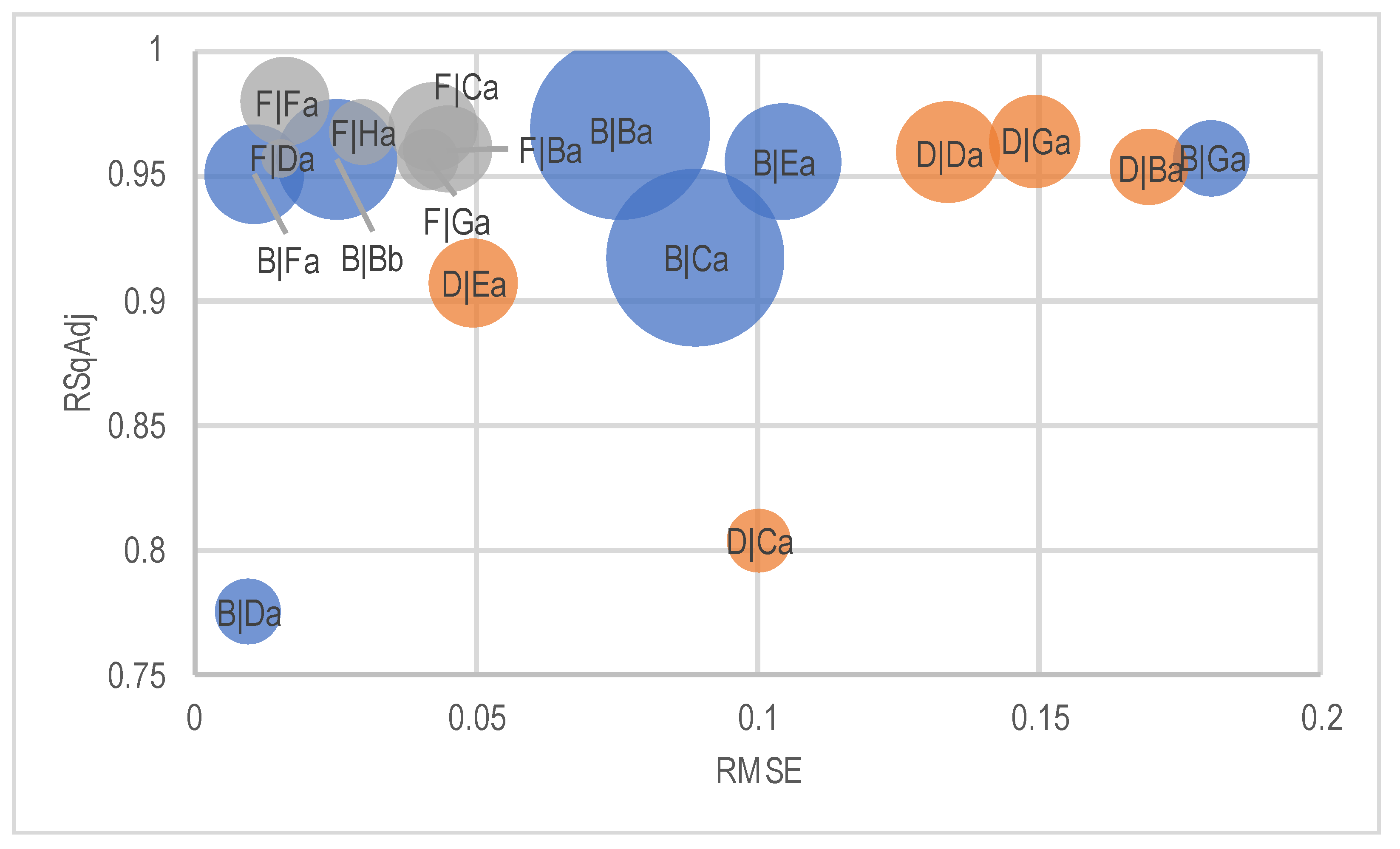
| Brand Identifier | Family Identifier | RMSE | RSqAdj | n |
|---|---|---|---|---|
| B | B|Ba | 0.0757 | 0.9689 | 202 |
| B|Bb | 0.0253 | 0.9569 | 88 | |
| B|Ca | 0.0889 | 0.9176 | 195 | |
| B|Da | 0.0096 | 0.7753 | 26 | |
| B|Ea | 0.1046 | 0.9557 | 85 | |
| B|Fa | 0.0107 | 0.9505 | 60 | |
| B|Ga | 0.1806 | 0.9574 | 35 | |
| D | D|Ba | 0.1696 | 0.9536 | 36 |
| D|Ca | 0.1002 | 0.8040 | 25 | |
| D|Da | 0.1339 | 0.9595 | 65 | |
| D|Ea | 0.0495 | 0.9075 | 49 | |
| D|Fa | 0.3279 | 0.9584 | 75 | |
| D|Ga | 0.1492 | 0.9639 | 51 | |
| F | F|Ba | 0.0450 | 0.9610 | 47 |
| F|Ca | 0.0425 | 0.9698 | 48 | |
| F|Da | 0.0153 | 0.9575 | 9 | |
| F|Fa | 0.0161 | 0.9799 | 48 | |
| F|Ga | 0.0415 | 0.9565 | 24 | |
| F|Ha | 0.0297 | 0.9680 | 26 |
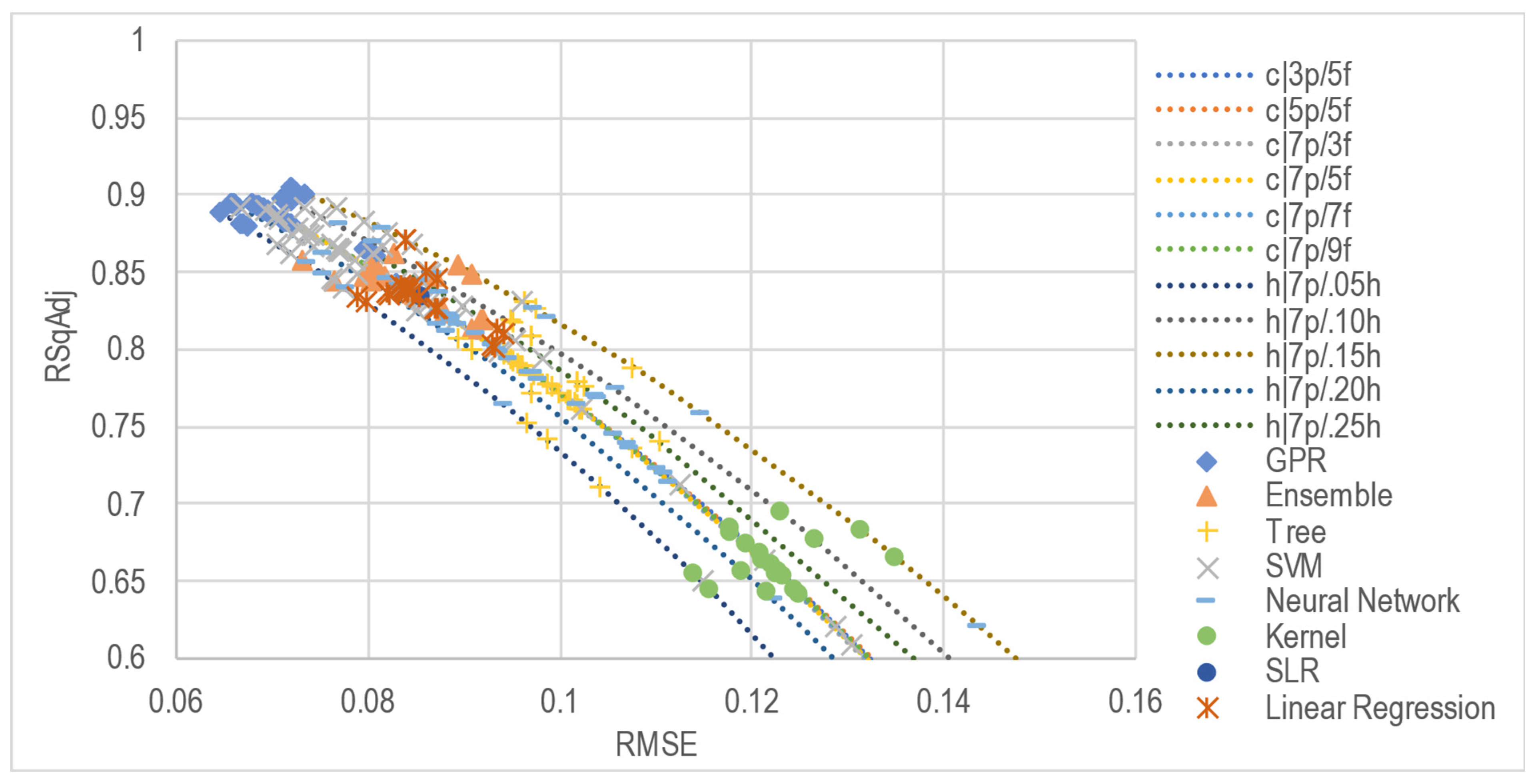
| Combine Family | Power Linear Regression | Machine Learning Optimized Gaussian Process Regression (GPR) | Observations | ||
|---|---|---|---|---|---|
| RMSE | RSqAdj | RMSE | RSqAdj | ||
| B|Bb | 0.0253 | 0.9569 | 0.0579 | 0.8970 | 88 |
| B|Da | 0.0096 | 0.7753 | 0.1027 | 0.1594 | 26 |
| B|Fa | 0.0107 | 0.9505 | 0.0806 | 0.7544 | 60 |
| F|Ba | 0.0450 | 0.9610 | 0.0806 | 0.6416 | 47 |
| F|Ca | 0.0425 | 0.9698 | 0.0710 | 0.7374 | 48 |
| F|Fa | 0.0161 | 0.9799 | 0.0539 | 0.9344 | 48 |
| F|Ga | 0.0415 | 0.9565 | 0.1231 | 0.7550 | 24 |
| F|Ha | 0.0297 | 0.9680 | 0.0313 | 0.9811 | 26 |
| Author | RMSE | RSqAdj | Observations |
|---|---|---|---|
| Cross and Perry (1995) [11] | 0.0988 | 0.7778 | 1197 |
| Unterschultz and Mumey (1996) [13] | 0.1040 | 0.5361 | 232 |
| Cross and Perry (1996) [12] | 0.1388 | 0.5615 | 1197 |
| Weersink and Stauber (1988) [9] | 0.1089 | 0.7301 | 1197 |
| Wu and Perry (2004) [14] | 0.1025 | 0.7609 | 1197 |
| ASABE D497.7 (2011 R2020) [16] | 0.1096 | 0.7264 | 1197 |
| Kay, Edwards and Duffy (2020) [15] | 0.1169 | 0.5720 | 924 |
| Herranz and Ruiz (2023) [24] | 0.0854 | 0.8342 | 1197 |
Disclaimer/Publisher’s Note: The statements, opinions and data contained in all publications are solely those of the individual author(s) and contributor(s) and not of MDPI and/or the editor(s). MDPI and/or the editor(s) disclaim responsibility for any injury to people or property resulting from any ideas, methods, instructions or products referred to in the content. |
© 2023 by the authors. Licensee MDPI, Basel, Switzerland. This article is an open access article distributed under the terms and conditions of the Creative Commons Attribution (CC BY) license (https://creativecommons.org/licenses/by/4.0/).
Share and Cite
Herranz-Matey, I.; Ruiz-Garcia, L. Agricultural Combine Remaining Value Forecasting Methodology and Model (and Derived Tool). Agriculture 2023, 13, 894. https://doi.org/10.3390/agriculture13040894
Herranz-Matey I, Ruiz-Garcia L. Agricultural Combine Remaining Value Forecasting Methodology and Model (and Derived Tool). Agriculture. 2023; 13(4):894. https://doi.org/10.3390/agriculture13040894
Chicago/Turabian StyleHerranz-Matey, Ivan, and Luis Ruiz-Garcia. 2023. "Agricultural Combine Remaining Value Forecasting Methodology and Model (and Derived Tool)" Agriculture 13, no. 4: 894. https://doi.org/10.3390/agriculture13040894