Article

Simulated Ecosystem and Farm-Level Economic Impacts of Conservation Tillage in a Northeastern Iowa County

1
Department of Agriculture Education and Communication, Tarleton State University, Stephenville, TX 76402, USA
2
Department of Accounting, Finance and Economics, Tarleton State University, Stephenville, TX 76402, USA
3
Center for Agricultural and Rural Development, Iowa State University, Ames, IA 50011, USA
4
Texas Institute for Applied Environmental Research, Tarleton State University, Stephenville, TX 76402, USA
*
Author to whom correspondence should be addressed.
Agriculture 2023, 13(4), 891; https://doi.org/10.3390/agriculture13040891
Submission received: 14 March 2023 / Revised: 13 April 2023 / Accepted: 17 April 2023 / Published: 18 April 2023
(This article belongs to the Special Issue Natural Resource and Environmental Economics in Agriculture)

Abstract

:
While the ecological benefits of no-till are largely indisputable, the economic impacts are less certain, and the latter may be partly to blame for lower-than-expected adoption of no-till. In this study, we contribute to a better understanding of the ecosystem and farm-level economic impacts of no-till, with Buchanan County in the northeastern region of the U.S. State of Iowa as the backdrop due to previously established data and model validation efforts in that region. Using the Agricultural Policy Environmental eXtender (APEX) and Farm Economic Model (FEM), we simulated two tillage scenarios—a conservation tillage baseline and no-till—for continuous corn and corn–soybean rotations in Buchanan County using gridded historical climate data. We find that no-till provides clear ecosystem benefits, except that soluble nutrient losses might actually rise. We also find that under current commodity prices for corn and soybeans, no-till is not as profitable as the conservation tillage baseline. For no-till to be at least as profitable as the baseline under current commodity prices, the yield penalty associated with no-till cannot be higher than 1.5% for corn and 0.8% for soybeans, or similar combinations that entail a revenue penalty of about $24,000 for an 809-hectare continuous corn or corn–soybean operation. Given the simulated yield penalties associated with no-till, corn and soybean prices would have to be substantially lower in order for no-till to break even. Consequently, incentives for conservation practice implementation may need to be tied to commodity prices and yield penalties in order to elicit greater adoption rates.

1. Introduction

Cultivated croplands are the predominant source of food and fiber for the global population, and this is in no small part due to advances in agronomic practices coupled with the use of high yielding varieties. However, croplands have also been implicated as a major source of nonpoint source pollution that impacts downstream waters [1,2]. Thus, many of the same advances in tillage and nutrient and pesticide applications that result in high-yielding crops have also been associated with significant nutrient, sediment, and chemical losses in surface runoff during storm events. For instance, hypoxia in the Gulf of Mexico has often been linked to nutrient and sediment losses in surface runoff from cultivated croplands upstream in the Mississippi River basin [1,3].
To mitigate these surface runoff and associated concerns, numerous structural and cultural practices have been implemented on cultivated croplands in the U.S. with varying degrees of success [4,5,6]. These practices, which have been partially funded by public programs, have often been buttressed by extensive field trials, though the actual post-implementation performance is usually less impressive, often due to a myriad of factors such as complex landscape issues, a lack of consistent and adaptive management, and even an unwillingness to invest time and effort due to a perceived risk of economic loss [6,7,8].

1.1. Disparities in Existing Studies on the Cost-Effectiveness of Conservation Tillage

Among the practices often promoted for mitigating nonpoint source pollution from cultivated croplands, conservation tillage has received great attention and has been widely implemented. A reason for the generally broad appeal for conservation tillage is that scientific advances in recent decades have made it easier for farmers to implement these practices. For instance, many farmers opt for no-till soybean production because of the wide availability of soybean varieties that are herbicide-ready. Thus, particularly for soybeans, no-till adoption rates have increased in recent decades. In fact, many farmers in Iowa already implement some form of conservation tillage as their default tillage practice for corn and soybean production [9,10].
Various studies have attempted to elucidate the impacts of conservation tillage on various ecological indicators. In general, these studies seem to yield a consensus that suggests a significant reduction in sediment losses in surface runoff, along with reductions in organic or sediment-bound nutrient losses (see, for instance, Ref. [11] for a review). The impacts on soluble nutrient losses are not as clear [12], and additional work is needed, not only to determine the direction of these impacts, but also to provide more robust estimates of the magnitudes.
While conservation tillage methods such as ridge till, no-till and strip till have been implemented more broadly than other recommended practices, their adoption rates are still lower than expected due to a lack of consistent data on the farm-level economic implications. For instance, while [10,13] indicated that no-till would result in a net cost to producers in a number of Iowa studies, Ref. [14] showed that no-till soybeans contributed substantially to overall profitability of a rice–soybean rotation in Arkansas. Furthermore, Ref. [15] found profit gains from no-till as compared to conventional tillage for rotations involving wheat, sorghum, and corn in Southwest Kansas. Similarly, Ref. [16] also found no-till to be more profitable than conventional tillage for corn production in northeastern Kansas. In Burleson County, Texas, Ref. [17] also found no-till to be preferred by risk-neutral and risk-averse producers for systems involving soybeans, wheat, and sorghum. Finally, experimental data from 1998 to 2002 on corn in nine states [18] showed that yields were on average lower, but profits were higher under no-till as compared to conventional tillage.
In contrast, similar to [10,13], Ref. [19] also found no-till to be less profitable than conventional tillage for many dryland cropping systems in the Great Plains. While the crops and the production regions differ, this disparity nonetheless illustrates the range of economic impacts in the literature for conservation tillage.
Many such disparities exist in the academic literature, and they exist even between studies covering the same crops, production regions, weather, and market conditions. Several key reasons exist for the disparities in economic impacts. First, no-till, for instance, is often associated in many studies with a yield penalty, at least in the initial years after implementation (see, for instance, Refs. [13,20]). Other studies, however, indicate a higher yield under no-till for soybean (e.g., Refs. [14,21,22]). Consequently, the farm-level economic implications of adopting no-till depends partly on the size of the yield penalty and the corresponding commodity prices. Secondly, the costs of field operations are also subject to substantial variability as evidenced by recent spikes in equipment and fuel prices. Additional reasons relate to the biophysical implications of conservation tillage practices including no-till, such as the practicability of performing or eliminating various field operations, an issue we return to later on. Thus, risk-averse farmers tend to maintain their status quo practices until there is overwhelming financial evidence in favor of the recommended practice change.
Owing in part to these disparities, there is a need to shed more light on the economic viability and cost-effectiveness of conservation tillage practices. In sum, contrasting the studies that address ecological impacts, most studies have failed to robustly ascertain the directional economic impact of conservation tillage. It is, in general, not known to a high degree of certainty whether a conservation tillage practice will entail a net profit or loss to the producer implementing the practice. As mentioned above, the lack of consensus regarding economic impacts of conservation practices is a major reason for less than anticipated adoption rates.

1.2. Previous Work That Informs the Present Study

This study is a contribution to the existing literature addressing the ecological and farm-level economic impacts of conservation tillage. We do not attempt here a robust synthesis of the subject. However, we contribute to a better understanding of this subject by presenting an assessment of no-till versus a baseline conservation tillage practice in an area that has been previously studied, but now in the current market context and within the broader context of the prevailing emphasis on ecosystem services. We explain our results in the appropriate context and, where necessary, highlight those aspects of the results that are fairly robust.
For this study, we leverage decades of watershed assessments and the development and application of linked economic-ecohydrological models for assessing conservation practice implementations. We utilize the widely used Agricultural Policy Environmental eXtender (APEX; Refs. [23,24,25]) ecohydrological model, and the Farm Economic Model (FEM; Ref. [26]), an annual farm-level economic simulator. These two models have been applied separately and jointly in many applications [26] and were specifically validated for the subject area of this study. In particular, APEX and FEM were utilized together with the Soil and Water Assessment Tool (SWAT; Refs. [24,27,28]) in the upper Maquoketa River watershed (UMRW) [9,10], a watershed in northeastern Iowa that covers portions of Buchanan, Clayton, Delaware and Fayette counties.
This study builds upon both earlier [9,10,29,30,31,32,33] and more recent [34,35,36,37,38,39,40,41,42,43,44] research. Various studies have evaluated the efficacy of APEX in simulating tillage practices and their resulting impacts on surface runoff, and sediment and nutrient losses. For instance, Refs. [9,10] focused on evaluating a number of conservation practices for cultivated croplands in the northeast Iowa region, while [34,44] assessed the impact of climate change on crop yields in Iowa and South Korea. Most recently, Ref. [35] projected the impacts of climate change on surface runoff and sediment and nutrient losses from cultivated croplands in Buchanan County. The practices evaluated by [9] and [10] included, among others, conservation tillage (specifically no-till), nutrient management, contour farming, terraces, buffer and filter strips, and various practice combinations. In that study, the models were calibrated and validated against measured ecological and agronomic (and, for FEM, economic) data prior to their use to simulate conservation practice implementation on croplands in a mixed crop–livestock farming region. The present study focusses only on Buchanan County, and highlights only conservation tillage to address no-till cost-effectiveness and standard ecological objectives including nutrient and sediment losses, and soil carbon sequestration.
We also build upon previous work conducted in the Fort Cobb Reservoir watershed in Oklahoma. In that application, the focus was on winter wheat production, and FEM was utilized to estimate the impact of implementing a no-till practice as opposed to the status quo distribution of tillage practices. In that study, no-till was found to entail an average net profit to farmers who implement it on their winter wheat fields in Oklahoma [45].
The previous studies in the UMRW [9,10] elucidated a number of facets of crop management in northeastern Iowa that informed the present study. First, the status quo tillage practice for continuous corn and corn–soybean rotations is already a form of conservation tillage. In general, conservation tillage is in widespread use across Iowa and much of the Corn Belt, prompting manufacturers to discontinue many lines of heavy tillage equipment in favor of minimum tillage options (see for instance, Ref. [46]). Thus, the baseline scenario to which [9,10] compared the no-till scenario was itself a form of conservation tillage. Second, farmers in that region who desire to implement no-till find it impracticable to fully eliminate all tillage operations. Thus, the scenario represented in [9,10] as no-till does not entail elimination of all tillage operations. Rather, it retains the row crop cultivation operation for corn. For these reasons, the results of [9,10], as well as this study, need to be understood in the context of incremental conservation tillage, rather than a contrast between conventional tillage and no-till.

1.3. Purpose of This Study

Given the foregoing, this study seeks to enhance our understanding of the ecological and farm-level economic impacts of conservation tillage in Buchanan County, Iowa. We build on the previous study in the UMRW [9,10] as well as the recent applications by [34], wherein climate change impacts on corn and soybean yields were determined and by [35], in which climate change impacts on surface runoff and sediment and nutrient losses were estimated for the same county. We also use the same models which have been validated previously for Buchanan County and many other study regions. The results of this study will enhance our understanding of the cost-effectiveness of incremental conservation tillage for cultivated croplands where reduced tillage is already practiced.
While the models and study area are similar, this study is distinct in terms of the microsimulation approach employed. We also utilize updated and more refined weather data, based on a 4 km grid as described briefly below and in [34,35]. We also cover all soil types within Buchanan County, thus enhancing transferability of the results to other areas within the U.S. Corn Belt.
While this study covers an entire county, it is, in reality, not a county-level study. We perform microsimulations simulating the diversity of soils, topography, weather and management practices represented in that county. Thus, in so far as similar soils, topography, weather, and cropping practices exist in other areas across the U.S. Midwest, the results of this study are broadly applicable to all those areas. The theoretical justification of this study is that by representing the variety of biophysical attributes in our simulations, we arrive at conclusions that are applicable not only to Buchanan County, but to the entire U.S. Corn Belt.

2. Materials and Methods

For this study, we leveraged decades of computer model development and application assets as well as extant data assembled for field scale, farm-level and watershed assessments across the United States. A brief description of the approach to evaluating conservation tillage impacts on ecosystem and farm-level economics follows, prior to presentation of the results.

2.1. Modeling System

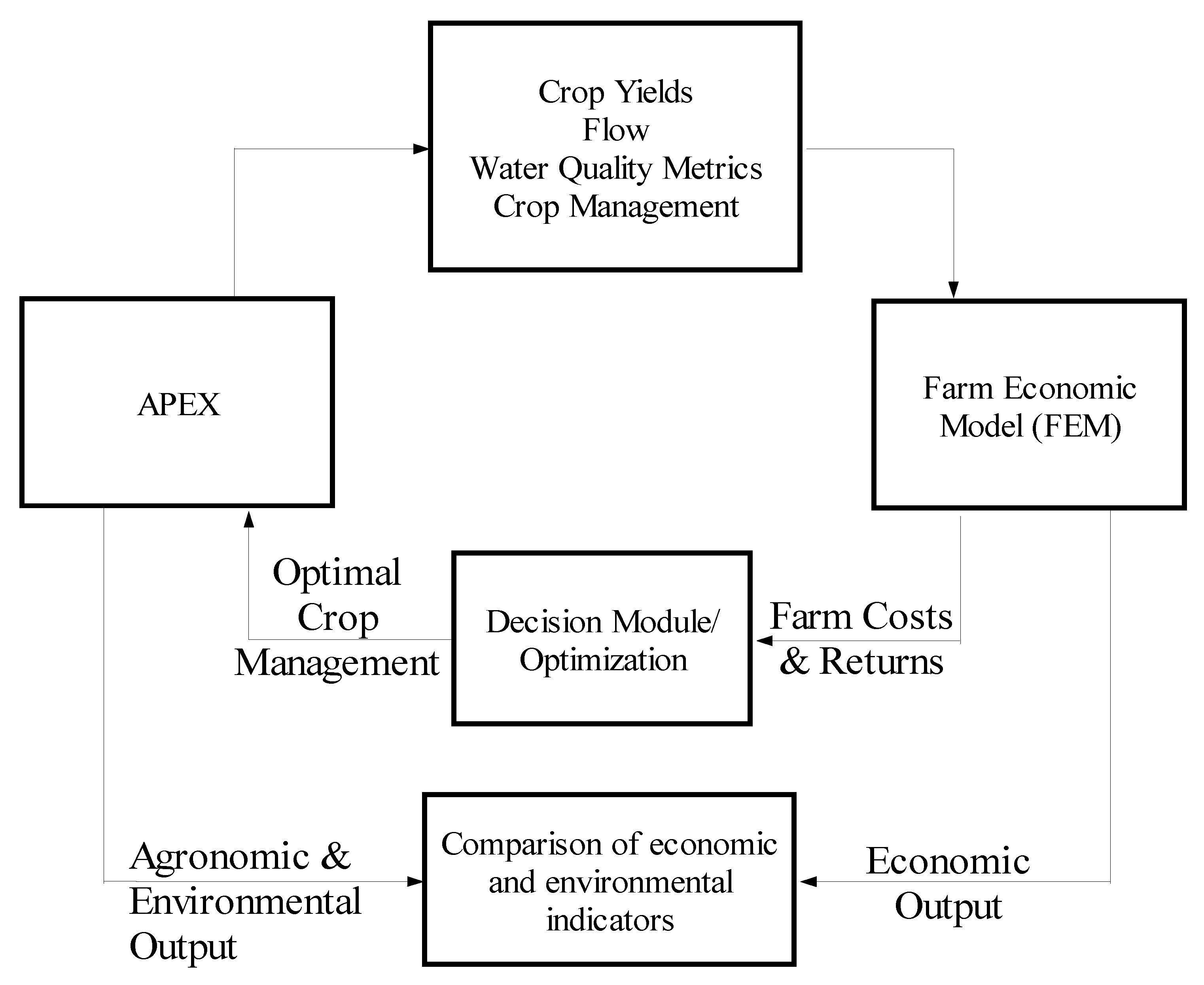
Two calibrated computer simulation models were used to simulate the ecosystem and farm-level economic impacts of conservation tillage in Buchanan County, Iowa. Both models were calibrated using historical weather, agricultural production data, farm cost and returns, and custom rate summaries. APEX was then used to simulate crop production, edge-of-field runoff, sediment and nutrient losses, and other ecological metrics under status quo and no-till practices. The crop productivity data obtained from the APEX simulations were then used as input in FEM [26,45], an annual economic simulation model for agricultural operations, to estimate the farm income and cost implications of the tillage practices simulated, and the crop production levels indicated by the APEX model. FEM is an annual economic simulation model that includes numerous subroutines and algorithms for simulating farm economics.
The two computer simulation models had been calibrated in previous efforts in Buchanan County, and were validated for the present study. FEM was used to determine the impacts of baseline tillage practices and no-till on farm incomes, costs, and net income. The APEX model was used to estimate crop yields and selected edge-of-field water quality metrics, namely sediment, total nitrogen, and total phosphorus in surface and subsurface flow. APEX was also used to estimate soil organic carbon levels and sequestration rates and other soil attributes. APEX and FEM have been linked in a previous effort to enable seamless transfer of data between the two models [26]. In this study the two models were applied in fully linked mode (Figure 1) to enable the transfer of biophysical parameters from APEX to the economic simulation model. The two models were calibrated separately prior to their use in the simulations.
APEX [23,24,25] is a comprehensive field-scale model that is a modified version of the Erosion Productivity Impact Calculator (EPIC) model [47]. Additional information describing the APEX application in this study is provided in [34]. APEX was calibrated against surface runoff data [48] as well as crop yield data assembled as part of the previous application [9,49].
Farm-level economic simulations were performed with the Farm Economic Model (FEM, Ref. [26]). FEM is a whole-farm annual economic model that simulates the economic impacts of a wide range of scenarios on farm enterprises based on applicable behavioral practices. The model was developed primarily for environmental policy assessment as part of a National Pilot Project on Livestock and the Environment (NPP, Ref. [26]), but is now widely applicable to a much broader range of agricultural policy assessments. FEM has been used in conjunction with APEX and SWAT to estimate the economic and environmental impacts of various policies and practices in several watersheds [10,26,35]. Both farm-level and watershed-scale impacts have been assessed. Recently, FEM was also integrated within a macro-modeling system that evaluates the economic and environmental impacts of agro-ecological practices across large geographic regions [50].
FEM simulates entire farms. Key components within the model include cropping systems and operations; livestock husbandry and nutrition; manure and waste management; equipment and machinery; types, sizes, and uses of land areas; structures and facilities; and exogenous factors. The cropping systems section of the model includes all aspects of crop management including field operations, input purchases, and grain and other product sales. The livestock systems section includes all livestock operations, nutrition, manure production characteristics, and livestock herd management. Special modules in FEM account for manure handling and storage, manure application on land, and other manure use or disposal options. All equipment, facilities and structures on the farm are accounted for in special modules that are designed to handle equipment purchase decisions and financing terms. Exogenous factors such as biophysical characteristics of the farm and government policy variables are also accounted for in the model.
Several FORTRAN routines within FEM estimate costs and returns of a farm based on livestock and crop operation schedules; ownership and the characteristics of structures, facilities, and equipment; financing terms; land areas and uses; livestock nutrition; manure production and handling; as well as other pertinent aspects of each farm enterprise. Optimizations required within the model are handled within a General Algebraic Modeling System (GAMS; Ref. [51]) submodule that is linked to special model routines for transfer of relevant decision and exogenous variables. FEM is discussed in greater detail in [26]. The following discussion is limited to components of the model that are directly related to evaluation of the tillage practices presented in this paper.
To estimate the economic impacts of alternative tillage systems the major cost and revenue components of relevance are grain sales, machinery repair and maintenance; fuel and lubrication; machinery ownership expenses (interest and depreciation); cost of hired and owner/operator labor; custom operation costs; and pesticide costs.
FEM permits very flexible specification of the field operations performed for a cropping system. Individual field operations can be specified for each crop in the rotation, each unique year of the rotation pattern, and each field that is unique in terms of crop management. For each operation, very flexible and detailed specifications can be provided. Field operation information includes the date of the operation, proportion of the field covered, frequency of the operation within the specified year, an indicator variable specifying whether the operation is custom hired or performed by the owner/operator, and an indicator specifying the types of fields the operation applies to. It also includes a list of input specifications detailing the machinery used for that operation, custom rates, seeding rates, herbicide use, and other crop input parameters. Furthermore, multiple implements can be specified for any field operation. The horsepower rating of the power implement determines hourly fuel and lubrication costs, while speed, width, and field efficiency of the implement determines how many hours are required for the operation.
The cost of a field operation is determined primarily by the hours required to complete that field operation. The hours required to complete a field operation on a hectare of land using a specific implement are given by
h = w s e θ 1
where h is the hours required per unit area of land, w is the width of the implement in meters, s is the field travel speed of the implement in km/hour, e is the implement field efficiency, and θ is a unit conversion constant equal to 10. In an operation involving multiple implements with different field travel speeds, widths, or field efficiencies, the hours per hectare of the operation is computed as the hours required for the slowest implement, i.e., the implement that covers the least amount of area per unit of time.
Once the hours of use are determined for a machine, its repair and maintenance, and fuel and lubrication expenses are based on agricultural machinery management specifications in ASAE EP496.1 [52,53] and ASAE D497.1 [54,55]. Specifically, repair and maintenance expenses for machinery j used in operation i in a given year t are given by (2), which is derived from the ASAE formula for cumulative repair and maintenance:
C j i t = h j i t h j t R F 1 j P j [ ( H j t 1000 ) R F 2 j ( H j t 1 1000 ) R F 2 j ]
where C j i t is the repair and maintenance expense for machinery j used in field operation i in year t ,
  • h j i t is the number of hours machinery j was used in field operation i in year t ,
  • h j t is the number of hours machinery j was used in all field operations in year t ,
  • R F 1 j and R F 2 j are ASAE repair and maintenance factors,
  • P j is the purchase price of machinery j , and
  • H j t is the cumulative hours of use of machinery j through the end of year t .
Fuel expenses are also computed in the model as a function of hours of use of each implement and various machinery coefficients [33,34,35,36]. Fuel cost per hour is given as
f h = c O g
where f h is the fuel cost per hour of use, c is a coefficient equal to 0.062 for gasoline engines and 0.045 for diesel powered engines, O is the horsepower rating for the power implement, and g is the fuel price per gallon. Fuel cost per hectare is obtained by dividing f h by the hectares covered per hour. Fuel cost per year is obtained by multiplying f h by the hours of implement use through the entire year. Oil and other lubrication expenses are expressed as a fixed ratio of fuel expenses based on the applicable ASAE Standards [52,53,54,55], which is typically 15% of fuel expenses.
Machinery ownership expenses are also computed in FEM and are partly dependent on use, since the expected economic life of each machine is typically expressed in hours. Hours of machinery use are used to compute the expected economic life in years within the model. Machinery depreciation expenses are inversely proportional to expected economic life. Interest and principal payments, on the other hand, are given as functions of exogenous borrowing terms.
Costs of hauling, drying, and handling are functions of crop yields. This study utilized hauling, drying, and handling costs reported in the Iowa State University crop production expenses for 2022 [56]. Harvesting costs, on the other hand, were simulated within the model. For continuous corn harvesting, the costs were determined based upon the machinery equations specified above. For corn–soybean harvesting, it was assumed that the producers would utilize custom harvesters since that is more cost-effective for the representative production area simulated, as compared to if the farmer had purchased the combine and grain heads and carts required and incurred the associated overhead, operating, and maintenance expenses.

2.2. Data Sources

Several data sources were used for this study. These data sources are described in greater detail in [34], and only mentioned here briefly.
Cropland data layer (CDL): This data layer was used to determine relevant corn and soybean growing areas in Buchanan County. It was obtained from the USDA–NRCS data server [57].
SSURGO soils data: The USDA–NRCS SSURGO soils data [58] was overlaid on the CDL data in order to determine the soil types applicable to 2021 corn and soybean production fields in Buchanan County. As detailed in [34], a total of 88,322 crop–soil polygons were simulated for continuous corn and 157,973 crop–soil polygons for corn–soybeans.
Weather data: Precipitation, minimum and maximum temperature, solar radiation, and other key weather variables were obtained from the USDA Parameter-elevation Regressions on Independent Slopes Model (PRISM) database [59]. The simulations presented here were performed with a 25-year time horizon of weather covering the 1981–2005 period. Additional details are provided in [34].
Crop management data: Based on the producer input detailed in [49], specific baseline field operations were defined for continuous corn and corn–soybean fields. Those operations are outlined in [
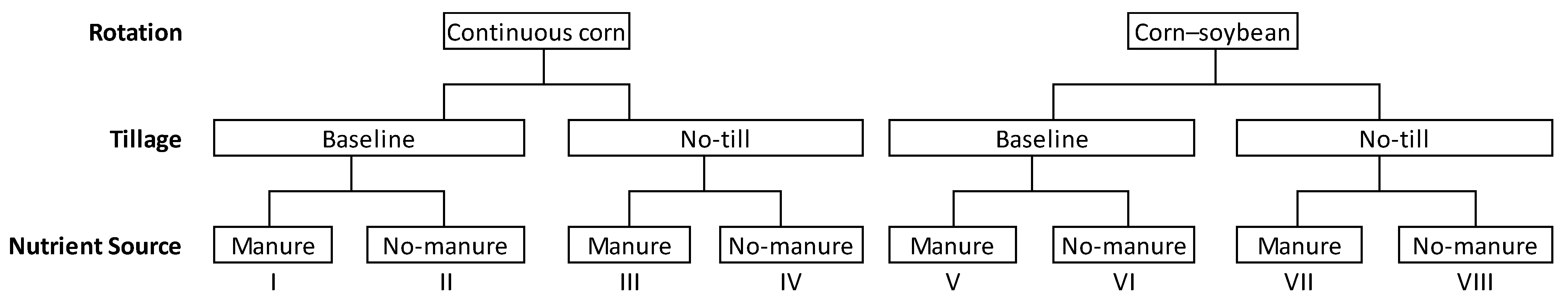
34] and represent a reduced tillage system. To simulate “no-till”, the field cultivator and chisel plow operations were eliminated. All other operations were retained, including the row cultivation operations, but a few dates were adjusted due to the timing of operations being slightly different when fewer tillage passes are performed. Field operations simulated for the “no-till” scenario are specified in Table 1 (for continuous corn) and Table 2 (for corn–soybean). The schedules in Table 1 and Table 2 represent no-till operations on fields receiving manure. For fields not receiving manure, the manure application operation was excluded and bulk spread operation on October 23 was changed to 28.0 + 30.0 + 55.8 (N+P+K) as in [34]. Very little crediting of manure nutrients occurred as discussed in [9,10,35]. Again, as outlined in [34], status quo tillage practices in the UMRW represented a reduced tillage style of management. Thus, the comparison between baseline and “no-till” is really a comparison between two conservation tillage scenarios; the baseline involving a few more tillage passes than the “no-till” scenario.

2.3. Representative Farms for Economic Simulations

Representative farms were specified in order to simulate the economic impacts of the tillage practices for appropriately sized operations. Each representative farm was specified as operating 809.4 ha of cultivated cropland, in addition to a small area for a farmhouse, equipment shed and other relevant buildings. A total of eight representative farms (I–VIII in Figure 2) were defined to account for replicates of two tillage options (baseline and no-till), two nutrient management options (manure-receiving fields and fields receiving only inorganic fertilizer), and two cropping systems (continuous corn and the corn–soybean rotation) (Figure 2). For the corn–soybean representative farm, the total area is divided into two equal halves, one planted in corn, and the other in soybean at any given point in time. For each representative farm, it was assumed that they owned only the minimum equipment and facilities required for their operation.
In previous applications where a variety of structural and livestock scenarios were evaluated, multiple farm sizes were represented in the simulations to capture the unique economic impacts that differ by size. However, this application only relates to tillage differences, in which case the difference in impacts is considerably dampened by the fact that smaller operations can utilize custom operators when owning capital intensive equipment is not cost-effective for them. Consequently, the farm-level economic impacts for tillage practices do not differ much by farm size. Thus, to simplify the study, only one farm size is utilized in this study: a total cropland area of 809 ha.

2.4. APEX Validation

For this study, the APEX output was compared to and calibrated against measured crop yields and edge-of-field ecological indicators. Details of APEX calibration results are reported in [34]. The results of the calibrations indicate that APEX was well-calibrated and validated for crop yield and environmental indicators (surface runoff, and sediment and nutrient losses) during the upper Maquoketa River watershed (UMRW) study [9]. APEX validations were also performed recently by [34,35] for the purposes of climate change simulations. Since we are utilizing the same model setup and study area, we consider it sufficiently validated for the current study.

2.5. FEM Validation

The economic model was also calibrated and validated for the UMRW study [9,10]. For the present study, we updated the model calibrations due to vastly different market conditions. FEM input parameters were adjusted within limits of acceptable economic and engineering coefficients, and equipment engineering coefficients were also adjusted accordingly. The original field machinery characteristics were obtained from [55,56,60], which were then adjusted during the calibration process. The resulting equipment prices and input coefficients relevant for this study are shown in Table 3, and were the input coefficients used in the FEM simulations.
During calibration, the performance of FEM was gauged using several goodness-of-fit metrics, chiefly the R2 statistic. The model was deemed adequately calibrated once total per hectare cost of each field operation was reasonably close to reported custom rate data [61]. For the most part, costs generated by the calibrated FEM model were within 2% of the reported custom rate average for the respective operation in the northeastern Iowa region. Regional custom rate data were used since inadequate data existed specifically for the relevant operations in Buchanan County. A comparison of the FEM simulated costs of field operations and the corresponding average custom rates are shown in Table 4.

2.6. Simulation Procedure

As in [34,35], 20% of crop–soil polygons identified as corn growing fields in Buchanan County in 2021 were simulated to determine the cost-effectiveness of no-till on continuous corn as compared to the baseline tillage system. Similarly, 20% of crop–soil polygons that were identified as corn or soybean growing fields in 2021 were simulated to evaluate no-till implementation in corn–soybean rotations as compared to the baseline tillage practice for the rotation. The rationale for using 20% of randomly selected crop–soil polygons is provided in detail in [34].
For each polygon, the baseline tillage presented in [34] was first simulated, followed by the no-till management depicted in Table 1 (for continuous corn) and Table 2 (for corn–soybean rotation). The key difference between the baseline and the no-till scenario was elimination of chisel plow and field cultivator operations for corn when the no-till scenario was simulated.

3. Results

Outputs from the APEX and FEM simulations were analyzed to determine the ecological and farm-level economic impacts of no-till when implemented on cultivated cropland, particularly continuous corn and corn–soybean rotations in Buchanan County. The APEX and FEM outputs provide a wide array of useful metrics. For this study, we will focus on five main classes of results:
  • Runoff and sediment losses;
  • Nutrient losses in surface runoff;
  • Carbon sequestration rates;
  • Corn and soybean yields;
  • Farm-level economic impacts.
As explained above, the baseline scenario represents a reduced tillage style of management. The alternative scenario simulated is a practical “no-till” scenario, which nonetheless, retains row crop cultivation on corn. Results are presented and discussed here on a per unit area basis and as percentage changes or per farm where applicable.

3.1. Impacts on Runoff and Sediment Losses

Relative to the reduced tillage baseline, no-till has minimal effect on surface runoff (Table 5). For both the baseline and the no-till scenario, surface runoff levels are similar between continuous corn and corn–soybean, and between fields receiving manure and those that do not. The area-weighted average surface runoff for the baseline is 133.5 mm/year, with a slightly higher rate for continuous corn than for corn–soybean, and a slightly lower rate for fields receiving manure than for those that receive only inorganic fertilizer.
Under the no-till scenario, surface runoff rates are slightly higher than under the baseline for continuous corn fields and lower on corn–soybean fields. Simulation results from APEX indicate that no-till results in a roughly 1% increase in surface runoff under continuous corn fields that do not receive manure, and 1.5% increase under continuous corn fields that do receive manure. In contrast, surface runoff rates are lower with no-till for corn–soybean fields, a roughly 2% reduction for both corn–soybean fields receiving manure and those that receive only inorganic fertilizer. Thus, the weighted average impact is a 1.4% reduction in surface runoff losses under no-till.
The impacts of no-till on sediment losses in runoff are markedly different. Results of the model simulations indicate that no-till would have a substantial impact on sediment losses in runoff as compared to the reduced tillage baseline. The greatest reduction in sediment losses is associated with the corn–soybean rotation when manure is utilized (close to 82% reduction), while the smallest impact is obtained for corn–soybean grown with only inorganic fertilizer (about a 61% reduction). No-till impacts on sediment losses for continuous corn with (about 70% reduction) and without (about 64% reduction) manure are intermediate. In summary, as expected based upon consistent results in the academic literature, sediment losses would decline significantly when no-till is practiced, relative to reduced tillage methods. Furthermore, the sediment loss reductions under no-till are greater on fields using manure than on fields that utilize only inorganic fertilizers.

3.2. Impacts on Nutrient Losses

Given that sediment losses are substantially reduced with no-till, we expect sediment-bound nutrients to also reduce under no-till. However, since surface runoff losses are only marginally changed, a reduction in soluble nutrient losses may be limited. The impacts of no-till on nutrient losses as compared to the baseline are displayed in Table 6 for nitrogen and phosphorus. The top panel of the table shows the baseline nutrient losses in kg/ha/year, followed by the middle panel, which displays the corresponding nutrient losses under no-till, and then the bottom panel, which shows the percentage changes in nutrient losses between the baseline and the no-till scenario.
As expected, sediment-bound nutrient losses are consistently and substantially reduced regardless of rotation and whether manure nutrients were utilized. Two results are consistent for sediment-bound nitrogen. First, the percentage reductions in sediment-bound nitrogen losses are somewhat greater in magnitude with continuous corn than with the corn–soybean rotation. Secondly, and more notably, the percentage reductions in sediment-bound nitrogen losses are greater on fields that do not receive manure than on fields that receive manure nutrients. The results are equally significant in magnitude, though not correspondingly, for sediment-bound phosphorus. In particular, we do not see consistently greater reductions for fields not receiving manure or for continuous corn fields. Rather, the reductions are greatest in magnitude for corn–soybean fields receiving manure, and secondarily—in terms of magnitude of the percentage changes—for continuous corn fields not receiving manure. The weighted-average percentage reductions in sediment-bound nitrogen and phosphorus losses are, respectively, 41% and approximately 50%. This compares favorably with the findings of [62] where nitrogen losses in sediment could be reduced by as much as 60% under no-till.
Under the baseline, sediment-bound nutrient losses are consistently greater than the corresponding soluble nutrient loss for both nitrogen and phosphorus regardless of rotation and whether manure is utilized on the fields. However, no-till impacts on sediment losses are so substantial that, for phosphorus, soluble nutrient losses under no-till are greater in magnitude than corresponding sediment-bound losses. However, no-till impacts on soluble N were considerably smaller relative to the corresponding phosphorus losses. In general, these results indicate the relative weakness of no-till in addressing soluble nutrient losses.
The results in Table 6 indicate that under no-till, soluble nutrient losses may not be reduced. In the case of phosphorus, soluble phosphorus losses actually increase under no-till. This phenomenon is actually well represented in the literature [63,64]. For instance, in previous efforts to reduce nutrient losses to Lake Erie [63], it was noted that while sediment-bound phosphorus losses declined with no-till, soluble phosphorus losses actually increased, very consistent with the results we find in this study. We see here, an average of 65% increase in soluble phosphorus losses when no-till is implemented. The increases are greater with fields receiving manure and with continuous corn.
No-till performance for soluble N losses is also less substantial than with sediment-bound N losses. However, the no-till scenario manages to register an area-weighted average reduction in soluble nitrogen losses of roughly 6%. Aside from corn–soybean fields not receiving manure, soluble nitrogen losses are reduced with no-till implementation. The reductions are greatest with continuous corn and with fields receiving manure.
Since for this application, sediment-bound nutrient losses are, in general, greater in magnitude than their soluble nutrient counterparts, there is generally a reduction in total N and total phosphorus losses with no-till, except for a small (less than 4%) increase in total phosphorus losses for continuous corn fields receiving manure, and essentially no impact (0% change) in total phosphorus losses for corn–soybean fields receiving manure. For total N losses, no-till registers a consistent reduction of about 50% regardless of rotation or whether the fields received manure nutrients. It is worth noting that the results may in part be predicated upon the baseline nutrient application rates. Future studies evaluating the implications of changes in the nutrient application rate on no-till effectiveness would be helpful.

3.3. Impacts on Carbon Sequestration

The implications of no-till for soil organic carbon content (SOC) and sequestration rates are shown in Table 7. Soil organic carbon and related changes in sequestration rates are indicated for four soil layer depths: 0.25 m, 0.5 m, 1.0 m, and 2.0 m. The numbers shown in the first two panels of the table reflect soil chemistry values at the end of the 25-year simulation period. The first panel of the table shows the model output for the baseline scenario. Each pair of numbers represents the soil organic carbon level in that depth of soil in mt/ha, followed by the same SOC level expressed as a percentage of total soil mass for the same depth. The second panel of the table shows corresponding values for the no-till scenario, followed by a third panel that indicates the percentage changes of the no-till soil organic carbon values from corresponding baseline values. The last panel shows the implied changes in SOC sequestration rates from the baseline, expressed in mt/ha/year.
It is clear from the results presented in Table 7 that manure applications enhance soil organic carbon levels. For both baseline and no-till scenarios, and regardless of rotation or depth of soil, fields receiving manure are associated with notably higher SOC levels at the end of the 25-year simulation horizon. The results also indicate that with or without manure, continuous corn fields have slightly higher soil organic matter levels than corn–soybean fields. We did not explore the reason for this latter finding as it is not the focus of this study, but it is likely due to the higher biomass levels on corn fields as compared to soybean fields after harvest.
The results of the simulations indicate consistent impacts of no-till on all fields simulated. No-till results in distinct, though modest, increases in SOC levels. The percentage changes further underscore that the increases in soil organic carbon levels are more pronounced for fields receiving manure. The improvements in SOC associated with no-till are largely confined to the top 0.5 m. However, as the results displayed here for soil layer depths are cumulative, the SOC levels and percentages show improvements under no-till for all depths.
Absolute sequestration rates are not reported in this paper. However, relative to the baseline, we report that carbon sequestration rates would increase by roughly 0.3 mt/ha/year for continuous corn or corn–soybean fields receiving manure, and about 0.1 mt/ha/year for fields that do not receive manure. As indicated above, the changes in sequestration rates are somewhat higher for continuous corn. The resulting area-weighted average changes in sequestration rates—averaged across both rotations and nutrient sources—are around 0.12 mt/ha/year for all soil layers, indicating that the changes are largely restricted to the top layer.

3.4. Impacts on Corn and Soybean Yields

Simulated crop yield impacts in response to no-till are shown in Table 8 in comparison to the baseline. Baseline continuous corn, corn following soybean, and soybean yields are shown in mt/ha/year in the first panel of the table, followed by corresponding yields under no-till in the second panel, and then percentage changes of no-till yields from baseline values in the last panel. As mentioned previously, baseline crop yields were validated recently in [26,34] and were shown to be consistent and robust indicators of the measured yields for the study area.
No-till implementation is shown to result in small reductions in corn and soybean yields. Note that other studies (e.g., Ref. [13]) indicated more sizable reductions in yields under no-till, but those reported reductions were for a few select years, as opposed to the 25-year annual average we report here. For continuous corn or corn following soybean, the yield reductions are in the range of roughly 4.7% as compared to the baseline. In contrast, soybean yields are expected to decline by roughly 2% under no-till. These yield-results reflect both long-term averages and the fact that soybean management under no-till is only one tillage operation removed from the baseline, whereas corn management under no-till is two or three tillage operations removed from the corresponding baseline.
It is important to emphasize that these yield impacts are based on annual average yields over the 25-year simulation horizon. As such, we did not account for the dynamic impacts of no-till over a longer time horizon, when improvements in soil organic matter are expected to result in improved yields under no-till. However, the average yield penalties reported here are supported by other studies (e.g., Refs. [65,66]) that indicate similar reductions under no-till corn production as compared to conventional tillage practices.

3.5. Farm-Level Economic Impacts

Farm-level economic impacts of the alternative tillage practices are contrasted in Table 9. As mentioned above in Section 2.3, only one farm size is represented here because the results for tillage alternatives are not expected to differ much by farm size, since farmers can choose to perform operations themselves or hire it out to a custom operator. The economic impacts of no-till as compared to the baseline hinge on two main factors: the impact of no-till on crop yields and hence total revenues, and the impacts of no-till on the costs of field operations as compared to the baseline. The results presented in Table 9 show that due to the yield penalty indicated for no-till as compared to the baseline, there is a substantial revenue reduction on an average annual basis. The revenue impacts of no-till are the most severe for continuous corn grown without manure (a roughly $102,000 average annual reduction in total revenue per farm), and least for corn–soybean fields where manure is not applied (close to a $67,000 average annual reduction per farm in that case).
Total costs are lower with no-till largely because of the elimination of the field cultivation and/or chisel plow operations for corn. However, the no-till planter is somewhat more expensive, thus reducing to some extent, the cost advantage of the fewer field operations. Nonetheless, no-till is shown to consistently result in reduced costs for both rotations with and without manure utilization.
Ultimately, net incomes are lower for no-till because the revenue reduction due to the yield penalty is of a much greater magnitude than the cost reduction due to fewer field operations. The net income reduction per hectare associated with no-till ranges from $17 for corn–soybean with manure to over $93 for continuous corn with manure. Based on the land area distributions for the two rotations and for fields utilizing manure versus those using only inorganic fertilizer, the average annual weighted average farm-level economic impact of no-till per hectare is $58.09.
Breakeven Corn and Soybean Prices
Since a key factor influencing the relative economic impacts is the yield penalty associated with both crops, it stands to reason that corn and soybean prices also play a major role in determining the relative economic impacts of no-till versus other tillage practices. In fact, a key reason for the farm-level economic impacts we report here is the relatively high levels of current corn and soybean prices, which, similar to most commodities, are at historic highs. Due to the yield penalty under no-till as compared to the baseline, lower corn and soybean prices would make no-till relatively more competitive. To shed better light on this, we provide a brief breakeven analysis below.
Given commodity prices P c and P s for corn and soybean, respectively, and total production costs C b and C n , respectively for the baseline (b) and no-till (n), the continuous corn (cc) and corn following soybean (cs) yields y c c b , y c s b , y c c n and y c s n for the baseline and no-till, and corresponding soybean yields y s b and y s n for the baseline and no-till, the breakeven condition between no-till and the baseline is simply defined as:
P c y c c b + P c y c s b + P s y s b C b P c y c c n + P c y c s n + P s y s n C n = 0
Equation (4) implies a breakeven commodity price relation between corn and soybean as represented in (5):
P s = C b C n P c y c c b + y c s b y c c n y c s n y s b y s n
Thus, the greater the cost reduction benefit of no-till, C b C n , the greater the range of plausible corn and soybean prices that are associated with economic breakeven, and by inference, the greater the economic performance of no-till as compared to the baseline. Similarly, the lower the yield penalty associated with no-till corn, ( y c c b + y c s b y c c n y c s n ) , or soybeans, y s b y s n , the greater the range of commodity prices consistent with breakeven and hence, no-till profitability. At the weighted average cost benefit of under $25,000 per year and simulated yield penalties, current commodity prices are too high for no-till to break even under these conditions, as compared to the baseline.
For additional insights, Figure 3 displays a graph of the breakeven corn and soybean prices conditioned upon six alternative weighted average corn and soybean yield penalties and cost reductions associated with no-till. The regions below each graph indicate the range of possible corn and soybean price combinations that are relatively profitable for no-till; the line graph itself is the breakeven frontier. Conversely, the regions above each line graph indicate the corn and soybean price combinations that are associated with no-till being less profitable than the baseline. In addition to the alternative cost and yield assumptions, we also display the simulated yield penalties and no-till cost reductions, labeled as “Current”, the lowest graph, closest to the origin. The actual corn and soybean prices are also plotted in the figure as the large dot (corresponding to $265.20/mt for corn and $546.30/mt for soybeans), far above the “Current” graph, and below only two graphs, both corresponding to 2.2% corn and 1.9% soybean yield penalties, respectively, with no-till: line graph D ($40,000 cost savings with no-till) and line graph E ($45,000 cost savings with no-till).
It is thus clear that in order for no-till to be more profitable than the baseline at the simulated yields and costs, corn and/or soybean prices would have to be significantly lower than their current levels. On the contrary, given current corn and soybean prices and the cost reduction associated with no-till, the breakeven yield penalties for corn and soybean are approximately 1.5% and 0.8%, respectively, or similar combinations that entail a revenue penalty of about $24,000 per 809-hectare continuous corn or corn–soybean operation. Under current prices, any yield penalties higher than these levels would result in a profit loss under no-till as compared to the reduced tillage baseline that is the status quo in northeastern Iowa for the continuous corn and corn–soybean rotations.

4. Discussion

The results of this study show that the economic impacts of no-till or other tillage practices hinge on three readily explicable factors: direct cost implications of changes in tillage practices, potential yield penalties associated with the tillage practice changes, and prevailing commodity prices. No-till is invariably associated with a reduction in the cost of field operations. However, if it is also associated with a yield penalty, the net effect on farm economics hinges on the magnitude of the yield penalty and the corresponding commodity prices. For this study, no-till was found to be less profitable than the conservation tillage baseline because the cost reduction afforded by the reduced tillage operations was not enough to offset the revenue reduction that results from the yield penalty and the high commodity prices. In general, if there is no yield penalty associated with no-till, there are clear economic benefits. If there is a yield penalty associated with no-till, then the economic impact hinges on the magnitude of the yield penalty and cost reductions as well as prevailing commodity prices.
The ecosystem benefits of no-till are undeniable. There are definite benefits in terms of sediment loss reduction and associated reductions in sediment-bound nutrients. However, soluble nutrient losses may not decline, and may in fact increase. For this reason, no-till may need to be implemented in combination with other practices that perform better at reducing soluble nutrient losses.
No-till is also beneficial for soil organic carbon sequestration. SOC levels increase appreciably with no-till, even over the levels associated with the conservation tillage baseline. With an increase in interest in climate-smart practices and monetization of other associated ecosystem services, no-till profitability may yet improve as farmers obtain additional sources of income for implementing no-till production practices.
The results of this study have clear policy implications. If no-till entails a net-income loss as is the case with current commodity prices and simulated yield penalties, financial incentives may be necessary to encourage adoption among producers. In devising such incentives, it is important for the government or other sponsoring agencies to tie these incentives to the commodity prices in order to better capture the magnitude of net-income loss, resulting in part from yield penalties.
While the study is set within the context of a northeastern Iowa county, the results are readily transferrable to other midwestern States. This direct transferability is due to the fact that while we utilized data pertaining to Buchanan County, we performed microsimulations that covered every soil type, weather, and topography applicable to the area. Thus, the results are applicable to any areas where similar soil types, topography, weather, and management practices prevail. Consequently, we expect that, with very few exceptions, the results are broadly applicable to similar conditions across much of the western Corn Belt region.
There are a number of limitations of this study. First, the management practices utilized in this study were based on producer surveys conducted around the year 2000. While current data indicate that the tillage practices are practically unchanged, nutrient applications have changed more considerably, with a greater emphasis on inorganic fertilizers than previously was the case. Second, while it is true that our model simulations indicate a moderate yield penalty with no-till, we did not address the inherent dynamics in soil chemistry over time that could eventually eliminate the yield penalty as soil productivity improves under no-till, as compared to the baseline. Other studies do support the notion that no-till is associated with a small-to-moderate yield penalty in many instances. Third, while we performed microsimulations over all soil types represented in Buchanan County, we acknowledge that the results of the study may not be directly transferrable to some areas in the Midwest where the soils, topography and climate are markedly different. In this case, though, we do maintain that the soil series and associated characteristics are quite representative to a good portion of the western Corn Belt region, and consequently the results of this study would be broadly applicable in those areas. Finally, while this is not a major limitation, we utilized only one farm size in the studies. The difference in impacts across farm size categories would be rather small when these impacts are expressed in $/ha. However, economic impacts expressed as percentage changes would definitely differ markedly due to the lower net income base of smaller operations.

5. Conclusions

No-till has often been promoted as a practice that will reduce nutrient and sediment runoff from cultivated croplands and increase SOC levels. It is also touted to retain topsoil productivity and consequently long-term crop yields. However, the farm-level economic implications are less certain. In this study, we explored the ecosystem and farm-level economic impacts of no-till in a northeastern Iowa county that has been studied extensively and benefited from economic and ecohydrological model calibrations. The objective was to contribute a more robust understanding of the economic implications as well as additional information on the associated ecosystem benefits.
Using well-calibrated ecohydrological (APEX) and economic (FEM) models, we simulated no-till and baseline tillage practices for continuous corn and corn–soybean rotations in Buchanan County, Iowa. The simulations were performed using SSURGO soils data and satellite imagery from the USDA’s CDL data sets to determine relevant soils associated with continuous corn and corn–soybean production.
The results of the simulations buttressed the fact that no-till provides clear ecosystem service benefits. While impacts on surface runoff volumes are negligible, there are clear benefits in terms of sediment loss reduction when no-till is implemented as compared to a conservation tillage baseline that entails only two or three additional tillage passes per year, relative to no-till. There are also corresponding benefits in relation to reductions in sediment-bound nutrient losses, which also see significant reductions.
In contrast, no-till does not appear to provide any benefits with respect to soluble nutrient losses. For both soluble N and soluble phosphorus, and the latter in particular, one could see significant increases in losses in surface runoff when no-till is implemented. This phenomenon is well-documented and our study provides confirmation of this finding. However, we also note that the levels of soluble nutrient losses may be predicated upon the rates of nutrient application utilized on the fields, an issue that deserves further study, but is beyond the scope of this paper.
Farm-level economic simulations indicate that no-till is currently not as profitable as the conservation tillage baseline. This is because while no-till results in a reduction in the costs of field operations, this reduction is not high enough to offset the revenue reduction that results from a 4.7% yield penalty for corn and a 2.3% yield penalty for soybeans, along with the historically high corn and soybean prices. A yield penalty no higher than 1.5% for corn and 0.8% for soybean would ensure that no-till is at least as profitable under current commodity prices and field operations costs. Additional efforts to synthesize the economic implications of alternative tillage practices will serve to reduce the perceived risk that is often at the heart of lower-than-expected adoption rates.

Author Contributions

E.O. played the leading role in design of the research, model calibration and validation, model simulations, initial writeup, and revisions. S.H.J. contributed to data assembly, review, and re-vision of writeup. P.W.G. contributed to initial model calibration and validation and revision of the writeup. A.S. contributed to model calibration, validation, and testing. All authors have read and agreed to the published version of the manuscript.

Funding

Funding for a portion of this research was provided by USDA to Project No. 2012-02355 through the National Institute for Food and Agriculture’s Agriculture and Food Research Initiative, Regional Approaches for Adaptation to and Mitigation of Climate Variability and Change.

Institutional Review Board Statement

Not applicable.

Informed Consent Statement

Not applicable.

Data Availability Statement

The data used for this study are all publicly available, and are cited in this paper. No restricted data were used in this paper.

Acknowledgments

The authors would like to acknowledge research support from Kimberly Ward, Regina Fontana, Alexis Hoang, Cori Salinas, and Sadie Woolery in preparation of some of the data used in this study.

Conflicts of Interest

The authors declare no conflict of interest.

References

  1. Carpenter, S.; Caraco, N.; Correll, D.; Howarth, R.; Sharply, A.; Smith, V. Nonpoint source pollution of surface waters with phosphorus and nitrogen. Ecol. Appl. 1998, 8, 559–568. [Google Scholar] [CrossRef]
  2. Xu, Y.; Elbakidze, L.; Yen, H.; Arnold, J.G.; Gassman, P.W.; Hubbart, J.; Strager, M.P. Integrated assessment of nitrogen runoff to the Gulf of Mexico. Resour. Energy Econ. 2022, 67, 101279. [Google Scholar] [CrossRef]
  3. Elizabeth, M.; Aillery, M.; Ribaudo, M.; Key, N.; Sneeringer, S.; Hansen, L.; Malcolm, S.; Riddle, A. Reducing Nutrient Losses from Cropland in the Mississippi/Atchafalaya River Basin: Cost Efficiency and Regional Distribution, ERR-258, U.S. Department of Agriculture, Economic Research Service, September 2018. Available online: https://www.ers.usda.gov/publications/pub-details/?pubid=90175 (accessed on 9 March 2023).
  4. Delgado, J.A.; Groffman, P.M.; Nearing, M.A.; Goddard, T.; Reicosky, D.; Lal, R.; Kitchen, N.R.; Rice, C.W.; Towery, D.; Salon, P. Conservation practices to mitigate and adapt to climate change. J. Soil Water Conserv. 2011, 66, 118A–129A. [Google Scholar] [CrossRef]
  5. Macrae, M.; Jarvie, H.; Brouwer, R.; Gunn, G.; Reid, K.; Joosse, P.; King, K.; Kleinman, P.; Smith, D.; Williams, M.; et al. One size does not fit all: Toward regional conservation practice guidance to reduce phosphorus loss risk in the Lake Erie watershed. J. Environ. Qual. 2021, 50, 529–546. [Google Scholar] [CrossRef]
  6. Roland, V.; Garcia, A.; Saad, D.; Ator, S.; Robertson, D.; Schwarz, G. Quantifying regional effects of best management practices on nutrient losses from agricultural lands. J. Soil Water Conserv. 2021, 77, 15–29. [Google Scholar] [CrossRef]
  7. Wallace, C.W.; Flanagan, D.C.; Engel, B.A. Quantifying the effects of conservation practice implementation on predicted runoff and chemical losses under climate change. Agric. Water Manag. 2017, 186, 51–65. [Google Scholar] [CrossRef]
  8. Garbrecht, J.D.; Nearing, M.A.; Shields, F.D., Jr.; Tomer, M.D.; Sadler, E.J.; Bonta, J.V.; Baffaut, C. Impact of weather and climate scenarios on conservation assessment outcomes. J. Soil Water Conserv. 2014, 69, 374–392. [Google Scholar] [CrossRef]
  9. Keith, G.; Norvell, S.; Jones, R.; Maquire, C.; Osei, E.; Saleh, A.; Gassman, P.; Rodecap, J. Livestock and The Environment: A National Pilot Project: CEEOT-LP Modeling for the Upper Maquoketa River Watershed, Iowa: Final Report; Report No. PR0003; Texas Institute for Applied Environmental Research, Tarleton State University: Stephenville, TX, USA, 2000. [Google Scholar]
  10. Gassman, P.W.; Osei, E.; Saleh, A.; Rodecap, J.; Norvell, S.; Williams, J. Alternative practices for sediment and nutrient loss con-trol on livestock farms in northeast Iowa. Agric. Ecosyst. Environ. 2006, 117, 135–144. [Google Scholar] [CrossRef]
  11. Palm, C.; Blanco-Canqui, H.; DeClerck, F.; Gatere, L.; Grace, P. Conservation agriculture and eco-system services: An overview. Agric. Ecosyst. Environ. 2014, 187, 87–105. [Google Scholar] [CrossRef]
  12. Daryanto, S.; Wang, L.; Jacinthe, P.A. Impacts of no-tillage management on nitrate loss from corn, soybean and wheat cultivation: A meta-analysis. Sci. Rep. 2017, 7, 12117. [Google Scholar] [CrossRef]
  13. Delate, K.; Cwach, D.; Chase, C. Organic No-Tillage System Effects on Soybean, Corn and Irrigated Tomato Production and Economic Performance in Iowa, USA. Renew. Agric. Food Syst. 2012, 27, 49–59. [Google Scholar] [CrossRef]
  14. Hristovska, T.; Watkins, K.B.; Anders, M.M. An economic risk analysis of no-till management for the rice-soybean rotation system used in Arkansas. J. Soil Water Conserv. 2013, 68, 132–137. [Google Scholar] [CrossRef]
  15. Norwood, C.A.; Currie, R.S. An Agronomic and Economic Comparison of the Wheat-Corn-Fallow and Wheat-Sorghum-Fallow Rotations. J. Prod. Agric. 1998, 11, 67–73. [Google Scholar] [CrossRef]
  16. Pendell, D.L.; Williams, J.R.; Rice, C.W.; Nelson, R.G.; Boyles, S.B. Economic feasibility of no-tillage and manure for soil carbon sequestration in corn production in northeastern Kansas. J. Environ. Qual. 2006, 35, 1364–1373. [Google Scholar] [CrossRef] [PubMed]
  17. Ribera, L.A.; Hons, F.M.; Richardson, J.W. An economic comparison between conventional and no-tillage farming systems in Burleson County, Texas. Agron. J. 2004, 96, 415–424. [Google Scholar] [CrossRef]
  18. Buman, R.A.; Alesii, B.A.; Hatfield, J.L.; Karlen, D.L. Profit, yield, and soil quality effects of tillage systems in corn–Soybean rotations. J. Soil Water Conserv. 2004, 59, 260–270. [Google Scholar]
  19. Dhuyvetter, K.C.; Thompson, C.R.; Norwood, C.A.; Halvorson, A.D. Economics of Dryland Cropping Systems in the Great Plains: A Review. J. Prod. Agric. 1996, 9, 216–222. [Google Scholar] [CrossRef]
  20. Toliver, D.K.; Larson, J.A.; Roberts, R.K.; English, B.C.; De La Torre Ugarte, D.G.; West, T.O. Effects of no-till on yields as influenced by crop and environmental factors. Agron. J. 2012, 104, 530–541. [Google Scholar] [CrossRef]
  21. Al-Kaisi, M.; Kwaw-Mensah, D. Effect of tillage and nitrogen rate on corn yield and nitrogen and phosphorus uptake in a corn-soybean rotation. Agron. J. 2007, 99, 1548–1558. [Google Scholar] [CrossRef]
  22. Al-Kaisi, M.; Licht, M.A. Effect of strip tillage on corn nitrogen uptake and residual soil nitrate accumulation compared with no-tillage and chisel plow. Agron. J. 2004, 96, 1164–1171. [Google Scholar] [CrossRef]
  23. Williams, J.R.; Arnold, J.G.; Kiniry, J.R.; Gassman, P.W.; Green, C.H. History of model development at Temple, Texas. Hydrol. Sci. J. 2008, 53, 948–960. [Google Scholar] [CrossRef]
  24. Williams, J.R.; Arnold, J.G.; Srinivasan, R. The APEX Model; BRC Report; No. 00-06; Blackland Research Center, Texas Agricultural Experiment Station, Texas Agricultural Extension Service, Texas A&M University System: Temple, TX, USA, 2000. [Google Scholar]
  25. Gassman, P.W.; Williams, J.R.; Wang, X.; Saleh, A.; Osei, E.; Hauck, L.M.; Izaurralde, R.; Flowers, J.D. Invited Review Article: The Agricultural Policy/Environmental eXtender (APEX) Model: An Emerging Tool for Landscape and Watershed Environmental Analyses. Trans. ASABE 2010, 53, 711–740. [Google Scholar] [CrossRef]
  26. Edward, O.; Gassman, P.; Saleh, A. Livestock and the Environment: A National Pilot Project: Economic and Environmental Modeling Using CEEOT.; Report No. PR0002; Texas Institute for Applied Environmental Research, Tarleton State University: Stephenville, TX, USA, 2000. [Google Scholar]
  27. Arnold, J.G.; Srinivasan, R.; Muttiah, R.S.; Williams, J.R. Large Area Hydrologic Modeling and Assessment Part I: Model Development. JAWRA J. Am. Water Resour. Assoc. 1998, 34, 73–89. [Google Scholar] [CrossRef]
  28. Arnold, J.G.; Moriasi, D.N.; Gassman, P.W.; Abbaspour, K.C.; White, M.J.; Srinivasan, R.; Santhi, C.; Harmel, R.D.; van Griensven, A.; Van Liew, M.W.; et al. SWAT: Model use, calibration, and validation. Trans. ASABE 2012, 55, 1491–1508. [Google Scholar] [CrossRef]
  29. Wang, X.; Williams, J.R.; Gassman, P.W.; Baffaut, C.; Izaurralde, R.; Jeong, J.; Kiniry, J.R. The EPIC and APEX models: Use, calibration and validation. Trans. ASABE 2012, 55, 1447–1462. [Google Scholar] [CrossRef]
  30. Tadesse, H.K.; Moriasi, D.N.; Gowda, P.H.; Marek, G.; Steiner, J.L.; Brauer, D.; Talebi-zadeh, M.; Nelson, A.; Starks, P. Evaluating evapotranspiration estimation methods in APEX model for dryland cropping systems in a semi-arid region. Agric. Water Manag. 2018, 206, 217–228. [Google Scholar] [CrossRef]
  31. Timlin; Dennis; Chun, J.A.; Meisinger, J.; Kang, K.; Fleisher, D.; Staver, K.; Doherty, C.; Russ, A. Evaluation of the agricultural policy environmental extender (APEX) for the Chesapeake Bay watershed. Agric. Water Manag. 2019, 221, 477–485. [Google Scholar] [CrossRef]
  32. Gautam, S.; Mbonimpa, E.G.; Kumar, S.; Bonta, J.V.; Lal, R. Agricultural Policy Environmental eXtender model simulation of climate change impacts on runoff from a small no-till watershed. J. Soil Water Conserv. 2015, 70, 101–109. [Google Scholar] [CrossRef]
  33. Ford, W.; King, K.; Williams, M.; Williams, J.; Fausey, N. Sensitivity Analysis of the Agricultural Policy/Environmental eXtender (APEX) for Phosphorus Loads in Tile-Drained Landscapes. J. Environ. Qual. 2015, 44, 1099–1110. [Google Scholar] [CrossRef]
  34. Osei, E.; Jafri, S.H.; Saleh, A.; Gassman, P.W.; Gallego, O. Simulated Climate Change Impacts on Corn and Soybean Yields in Buchanan County, Iowa. Agriculture 2023, 13, 268. [Google Scholar] [CrossRef]
  35. Osei, E.; Jafri, S.H.; Gassman, P.W.; Saleh, A.; Gallego, O. Climate Change Impacts on Surface Runoff and Nutrient and Sediment Losses in Buchanan County, Iowa. Agriculture 2023, 13, 470. [Google Scholar] [CrossRef]
  36. Kim, D.-H.; Jang, T.; Hwang, S. Evaluating impacts of climate change on hydrology and total nitrogen loads using coupled APEX-paddy and SWAT models. Paddy Water Environ. 2020, 18, 515–529. [Google Scholar] [CrossRef]
  37. Bailey, R.T.; Tasdighi, A.; Park, S.; Tavakoli-Kivi, S.; Abitew, T.; Jeong, J.; Green, C.H.; Worqlul, A.W. APEX-MODFLOW: A New integrated model to simulate hydrological processes in watershed systems. Environ. Model. Softw. 2021, 143, 105093. [Google Scholar] [CrossRef]
  38. Worqlul, A.W.; Jeong, J.; Green, C.H.M.; Abitew, T.A. The impact of rainfall distribution methods on streamflow throughout multiple elevations in the Rocky Mountains using the APEX model—Price River watershed, Utah. J. Environ. Qual. 2021, 50, 1395–1407. [Google Scholar] [CrossRef] [PubMed]
  39. Cheng, G.; Harmel, R.; Ma, L.; Derner, J.; Augustine, D.; Bartling, P.; Fang, Q.; Williams, J.; Zilverberg, C.; Boone, R.; et al. Evaluation of APEX modifications to simulate forage production for grazing management decision-support in the Western US Great Plains. Agric. Syst. 2021, 191, 103139. [Google Scholar] [CrossRef]
  40. Carroll, S.R.; Le, K.N.; Moreno-García, B.; Runkle, B.R.K. Simulating Soybean–Rice Rotation and Irrigation Strategies in Arkansas, USA Using APEX. Sustainability 2020, 12, 6822. [Google Scholar] [CrossRef]
  41. Mason, R.E.; Merrill, S.; Görres, J.; Faulkner, J.; Niles, M. Agronomic and environmental performance of dairy farms in a warmer, wetter climate. J. Soil Water Conserv. 2021, 76, 76–88. [Google Scholar] [CrossRef]
  42. Raj, A.D.; Kumar, S.; Sooryamol, K. Sooryamol. Modelling climate change impact on soil loss and erosion vulnerability in a watershed of Shiwalik Himalayas. Catena 2022, 214, 106279. [Google Scholar] [CrossRef]
  43. Kamruzzaman, M.; Hwang, S.; Choi, S.-K.; Cho, J.; Song, I.; Song, J.-h.; Jeong, H.; Jang, T.; Yoo, S.-H. Evaluating the Impact of Climate Change on Paddy Water Balance Using APEX-Paddy Model. Water 2020, 12, 852. [Google Scholar] [CrossRef]
  44. Mohammad, K.; Hwang, S.; Choi, S.-K.; Cho, J.; Song, I.; Jeong, H.; Song, J.-H.; Jang, T.; Yoo, S.-H. Prediction of the effects of management practices on discharge and mineral nitrogen yield from paddy fields under future climate using APEX-paddy model. Agric. Water Manag. 2020, 241, 106345. [Google Scholar] [CrossRef]
  45. Osei, E.; Moriasi, D.N.; Steiner, J.L.; Starks, P.J.; Saleh, A. Farm-Level Economic Impact of No-Till Farming in the Fort Cobb Reservoir Watershed. J. Soil Water Conserv. 2012, 67, 75–86. [Google Scholar] [CrossRef]
  46. Miller, D. Equipment Roundup: John Deere Discontinues 3710 Moldboard Plow. Progressive Farmer, DTN. 6/20/2022. Available online: https://www.dtnpf.com/agriculture/web/ag/equipment/article/2022/06/20/deere-retires-3710-moldboard-plow#:~:text=%22On%20July%208%2C%202022%2C,the%20995%20Reversible%20Moldboard%20Plow (accessed on 18 February 2023).
  47. Williams, J.R. The erosion-productivity impact calculator (EPIC) model: A case history. Philos. Trans. R. Soc. B Biol. Sci. 1990, 329, 421–428. [Google Scholar]
  48. USEPA. EnviroAtlas Data Download. National Table Downloads. Available online: https://www.epa.gov/enviroatlas/forms/enviroatlas-data-download (accessed on 11 November 2022).
  49. Osei, E.; Gassman, P.; Saleh, A. Livestock and the Environment: A National Pilot Project: CEEOT–LP Modeling for the Upper Maquoketa River Watershed, Iowa: Technical Report; Report No. RR0001; Texas Institute for Applied Environmental Research, Tarleton State University: Stephenville, TX, USA, 2000. [Google Scholar]
  50. Osei, E.; Bekele, A.; Du, B.; Rose, R.; Hauck, L.; Saleh, A.; Houser, J.; Keplinger, K.; Beran, L. CEEOT-MMS: A Macro Modeling System for Environmental Assessment; Technical Report TR0303; Texas Institute for Applied Environmental Research, Tarleton State Univ.: Stephenville, TX, USA, 2003. [Google Scholar]
  51. Brooke, A.; Kendrick, D.; Meeraus, A. GAMS: A User’s Guide; World Bank: Washington, DC, USA, 1992. [Google Scholar]
  52. ASAE. Agricultural Machinery Management. ASAE Engineering Practice: EP496.1, ASAE Standards; American Society of Agricultural Engineers: St. Joseph, MI, USA, 1995. [Google Scholar]
  53. ASABE. Agricultural Machinery Management. ASABE Engineering Practice: EP496.3, ASABE Standards; American Society of Agricultural Engineers: St. Joseph, MI, USA, 2006; Available online: https://elibrary.asabe.org/abstract.asp?aid=47748 (accessed on 29 January 2023).
  54. ASAE. Agricultural Machinery Management Data. ASAE Data: ASAE D497.1, ASAE Standards; American Society of Agricultural Engineers: St. Joseph, MI, USA, 1995. [Google Scholar]
  55. ASABE. Agricultural Machinery Management Data. ASAE Data: ASAE D497.5, ASABE Standards; American Society of Agricultural Engineers: St. Joseph, MI, USA, 2021; Available online: https://www.tractoresymaquinas.com/wp-content/uploads/2021/07/ASABE_D497.5.pdf (accessed on 29 January 2023).
  56. Plastina, A. Estimated Costs of Crop Production in Iowa. Iowa State University, Ames, Iowa. Ag Decision Maker. File A1-20. FM 1712 Revised January 2022. Available online: https://www.extension.iastate.edu/agdm/crops/pdf/a1-20-2022.pdf (accessed on 12 March 2023).
  57. USDA-NASS. USDA National Agricultural Statistics Service Cropland Data Layer; USDA-NASS: Washington, DC, USA, 2022. Available online: https://nassgeodata.gmu.edu/CropScape/ (accessed on 21 November 2022).
  58. USDA-NRCS. Soil Survey Staff, Natural Resources Conservation Service, United States Department of Agriculture. Soil Survey Geographic (SSURGO) Database. 2022. Available online: https://websoilsurvey.nrcs.usda.gov (accessed on 21 November 2022).
  59. PRISM Climate Group. PRISM Climate Group, Oregon State University. 2022. Available online: https://prism.oregonstate.edu (accessed on 21 November 2022).
  60. Lattz, D.; Schnitkey, G. Machinery Cost Estimates for 2021. FarmDoc Dly. 2021, 11, 143, Department of Agricultural and Consumer Economics, University of Illinois at Urbana-Champaign, 12 October 2021. [Google Scholar]
  61. Alejandro, P.; Ann; Johanns, M. Iowa Farm Custom Rate Survey. Iowa State University, Ames, Iowa. Ag Decision Maker. File A3-10. FM 1698 Revised March 2022. Available online: https://www.extension.iastate.edu/agdm/crops/html/a3-10.html (accessed on 12 March 2023).
  62. Edwards, K.A.; Foulger, M. A review of the efficacy of contemporary agricultural stewardship measures for ameliorating water pollution problems of key concern to the UK water industry. Agric. Syst. 2009, 99, 67–75. [Google Scholar]
  63. Jarvie, H.P.; Johnson, L.T.; Sharpley, A.N.; Smith, D.R.; Baker, D.B.; Bruulsema, T.W.; Confesor, R. Increased Soluble Phosphorus Loads to Lake Erie: Unintended Consequences of Conservation Practices? J. Environ. Qual. 2017, 46, 123–132. [Google Scholar] [CrossRef]
  64. Sharpley, A.N.; Daniel, T.; Gibson, G.; Bundy, L.; Cabrera, M.; Sims, T.; Stevens, R.; Lemunyon, J.; Kleinman, P.; Parry, R. Best Management Practices to Minimize Agricultural Phosphorus Impacts on Water Quality; ARS–163; United States Department of Agriculture, Agricultural Research Service: Washington, DC, USA, 2006. Available online: https://naldc.nal.usda.gov/catalog/26763 (accessed on 4 April 2023).
  65. Pittelkow, C.M.; Linquist, B.A.; Lundy, M.E.; Liang, X.; van Groenigen, K.J.; Lee, J.; van Gestel, N.; Six, J.; Venterea, R.T.; van Kessel, C. When does no-till yield more? A global meta-analysis. Field Crops Res. 2015, 183, 156–168. [Google Scholar] [CrossRef]
  66. Griffith, D.R.; Kladivko, E.J.; Mannering, J.V.; West, T.D.; Parsons, S.D. Long-Term Tillage and Rotation Effects on Corn Growth and Yield on High and Low Organic Matter. Poorly Drained Soils. Agron. J. 1988, 80, 599–605. [Google Scholar] [CrossRef]
Figure 1. Schematic of FEM and APEX linkage for scenario simulation and analysis.
Agriculture 13 00891 g001
Figure 2. Types of representative farms used in economic simulations.
Agriculture 13 00891 g002
Figure 3. Graphs of breakeven corn and soybean prices for no-till as compared to the baseline under alternative yield penalty and cost reduction assumptions.
Agriculture 13 00891 g003
Table 1. Field operations simulated for no-till continuous corn for 1998–2000 production years.
DateOperation *
16 AprilApply manure (44.9 MT/ha)
29 AprilApply herbicide
3 MayPlant
3 MayIncorporate starter fertilizer (kg/ha) (10.1 + 11.3 + 27.9)
12 JuneCultivate
18 OctoberHarvest corn
23 OctoberBulk spread (kg/ha) (17.9 + 20.2 + 41.9)
12 NovemberApply Ammonia (194.2 kg/ha)
Table 2. Field operations simulated for no-till corn–soybean rotation for 1998–2000 production years.
DateOperation
Corn following soybean
16 AprilApply manure (44.9 MT/ha)
29 AprilApply herbicide
29 AprilApply fertilizer N (128.2 kg/ha)
1 MayPlant corn
1 MayIncorporate starter fertilizer (kg/ha) (10.1 + 11.3 + 27.9)
12 JuneCultivate
15 OctoberHarvest corn
25 OctoberBulk spread (kg/ha) (17.9 + 20.2 + 41.9)
Soybean following corn
16 AprilApply manure (44.9 MT/ha)
29 AprilApply herbicide
10 MayField cultivate
12 MayPlant soybean
2 OctoberHarvest soybean
27 OctoberBulk spread (kg/ha) (15.4 + 17.3 + 41.9)
Table 3. Characteristics of field machines after FEM calibration *.
MachinePrice
($)
HoursWidth
(m)
Speed
(ms−1)
Field Eff.Horse-PowerRF1RF2
95 HP Tractor120,86612,800NANA80950.0032.0
240 HP Tractor284,69012,800NANA802400.0032.0
Bulk fert spreader: 7.6 m770025007.62.975NA0.631.3
Ammonia applicator—11.4 m99,663400011.43.490NA0.631.3
Sprayer61,776150027.42.665730.431.8
Chisel plow: 7 m55,66130007.02.685NA0.281.4
Row cultivator66,771250012.22.780NA0.172.2
Field cultivator—9 m71,10922009.02.785NA0.271.4
Planter, 8 row narrow52,26128006.12.985NA0.322.1
No-till planter64,18115006.12.970NA0.0072.0
Manure spreader26,23230004.63.085NA0.631.3
Corn Head, 8 row narrow83,00080006.72.085NA0.122.3
270 HP Combine339,2506000NANA852700.022.1
* NA implies not applicable.
Table 4. Costs of simulated field operations and corresponding custom rates: $/hectare.
Current Custom RateFEM Model Estimate
TotalVariable
Bulk fertilizer spreading15.2015.0710.06
Chisel plow44.4844.2126.51
Row cultivation31.0130.1516.41
Field cultivation39.2938.8220.31
Row planting51.8951.8934.10
No-till planting57.4556.6126.41
Ammonia application33.1129.0117.47
Manure applicationNA66.1234.72
Combine corn90.8190.9145.76
Herbicide spraying16.6817.157.31
Table 5. Conservation tillage impacts on annual surface runoff and sediment losses.
BaselineNo-TillPercentage Change
Rotation and ManagementSurface Runoff (mm)Sediment Losses (mt/ha)Surface Runoff (mm)Sediment Losses (mt/ha)Surface Runoff (%)Sediment Losses (%)
Corn without manure134.592.90135.751.030.9−64.4
Corn with manure133.791.63135.810.481.5−70.7
Corn–soybean without manure133.271.97130.470.76−2.1−61.3
Corn–soybean with manure132.931.01130.520.18−1.8−81.7
Area weighted average133.461.99131.530.72−1.5−63.6
Table 6. Conservation tillage impacts on nutrient losses in surface runoff (kg/ha/yr) *.
Rotation and ManagementSoluble NSediment-Bound NTotal NSoluble PSediment-Bound PTotal P
Baseline
Corn without manure6.5816.1722.750.722.273.00
Corn with manure10.0955.6865.771.912.824.73
Corn–soybean without manure4.4111.7116.120.781.632.40
Corn–soybean with manure6.7848.7955.572.082.644.72
Area weighted average5.2618.7223.980.971.912.88
No-till
Corn without manure4.997.0312.021.241.082.31
Corn with manure7.2038.3645.563.501.394.89
Corn–soybean without manure4.615.7110.321.220.882.10
Corn–soybean with manure6.1636.1842.343.651.074.72
Area weighted average4.9510.9615.921.610.952.57
Percentage changes from baseline
Corn without manure−24.3−56.5−47.270.8−52.7−22.8
Corn with manure−28.7−31.1−30.783.2−50.63.5
Corn–soybean without manure4.5−51.2−36.056.8−45.9−12.7
Corn–soybean with manure−9.1−25.9−23.875.3−59.5−0.1
Area weighted average−5.9−41.4−33.665.4−49.9−10.9
* Capital P in this table refers to phosphorus. Elsewhere, italicized P with a subscript refers to a commodity price.
Table 7. Conservation tillage impacts on soil organic carbon.
Rotation and ManagementDepth of Soil Layer
0.25 m0.5 m1 m2 m
Baseline (mt/ha [%])
Corn without manure120.9 [3.27]215.7 [2.86]302.0 [1.89]352.7 [1.11]
Corn with manure135.9 [3.68]231.3 [3.07]317.9 [1.99]368.8 [1.16]
Corn–soybean without manure120.4 [3.26]215.1 [2.85]301.0 [1.89]351.8 [1.11]
Corn–soybean with manure137.2 [3.71]232.1 [3.08]318.1 [1.99]369.0 [1.16]
Area weighted average123.2 [3.33]218.0 [2.89]303.9 [1.90]354.8 [1.12]
No-till (mt/ha [%])
Corn without manure123.9 [3.31]219.0 [2.89]305.4 [1.91]356.2 [1.12]
Corn with manure144.2 [3.86]239.4 [3.16]325.9 [2.04]376.7 [1.19]
Corn–soybean without manure122.3 [3.27]217.0 [2.86]302.8 [1.89]353.6 [1.11]
Corn–soybean with manure144.5 [3.86]239.3 [3.15]325.1 [2.03]375.9 [1.18]
Area weighted average126.2 [3.37]220.9 [2.91]306.9 [1.92]357.7 [1.12]
Percentage changes from baseline
Corn without manure2.51.51.11.0
Corn with manure6.13.52.52.1
Corn–soybean without manure1.60.90.60.5
Corn–soybean with manure5.33.12.21.9
Area weighted average2.41.41.00.8
Change in soil carbon sequestration rate (mt/ha/yr)
Corn without manure0.120.130.140.14
Corn with manure0.330.320.320.32
Corn–soybean without manure0.080.070.070.07
Corn–soybean with manure0.290.280.280.28
Area weighted average0.120.120.120.12
Table 8. Conservation tillage impacts on corn and soybean yields (mt/ha/year).
Rotation and ManagementCorn Following CornCorn Following SoybeanSoybean
Baseline
Corn without manure8.40
Corn with manure8.45
Corn–soybean without manure 8.453.17
Corn–soybean with manure 8.463.17
Area weighted average8.418.453.17
No-till
Corn without manure7.99
Corn with manure8.05
Corn–soybean without manure 8.063.09
Corn–soybean with manure 8.073.10
Area weighted average8.008.063.10
Percentage changes from baseline
Corn without manure−4.9
Corn with manure−4.7
Corn–soybean without manure −4.6−2.3
Corn–soybean with manure −4.7−2.3
Area weighted average−4.9−4.6−2.3
Table 9. Average annual conservation tillage impacts on farm-level economics ($/year).
Total Revenue ($/Farm)Total Cost ($/Farm)Net Income ($/Farm)Net Income per Hectare ($/ha)
Baseline
Corn without manure$2,111,081$1,912,136$198,945$245.80
Corn with manure$2,123,011$1,923,390$199,621$246.63
Corn–soybean without manure$1,858,562$1,560,999$297,562$367.64
Corn–soybean with manure$1,860,690$1,586,248$274,442$339.07
Area-weighted average$1,909,718$1,634,902$274,816$339.53
No-till
Corn without manure$2,008,292$1,881,208$127,084$157.01
Corn with manure$2,022,481$1,898,650$123,832$152.99
Corn–soybean without manure$1,791,821$1,540,188$251,633$310.89
Corn–soybean with manure$1,792,532$1,531,972$260,560$321.92
Area-weighted average$1,835,652$1,607,854$227,797$281.44
Impact of no-till
Corn without manure$102,789$30,928$71,861$88.78
Corn with manure$100,530$24,740$75,789$93.64
Corn–soybean without manure$66,741$20,812$45,929$56.75
Corn–soybean with manure$68,157$54,276$13,882$17.15
Area-weighted average$74,066$27,048$47,019$58.09
Disclaimer/Publisher’s Note: The statements, opinions and data contained in all publications are solely those of the individual author(s) and contributor(s) and not of MDPI and/or the editor(s). MDPI and/or the editor(s) disclaim responsibility for any injury to people or property resulting from any ideas, methods, instructions or products referred to in the content.

