Agricultural Land Use Changes as a Driving Force of Soil Erosion in the Velika Morava River Basin, Serbia

 , , , and
Abstract
:1. Introduction
2. Materials and Methods
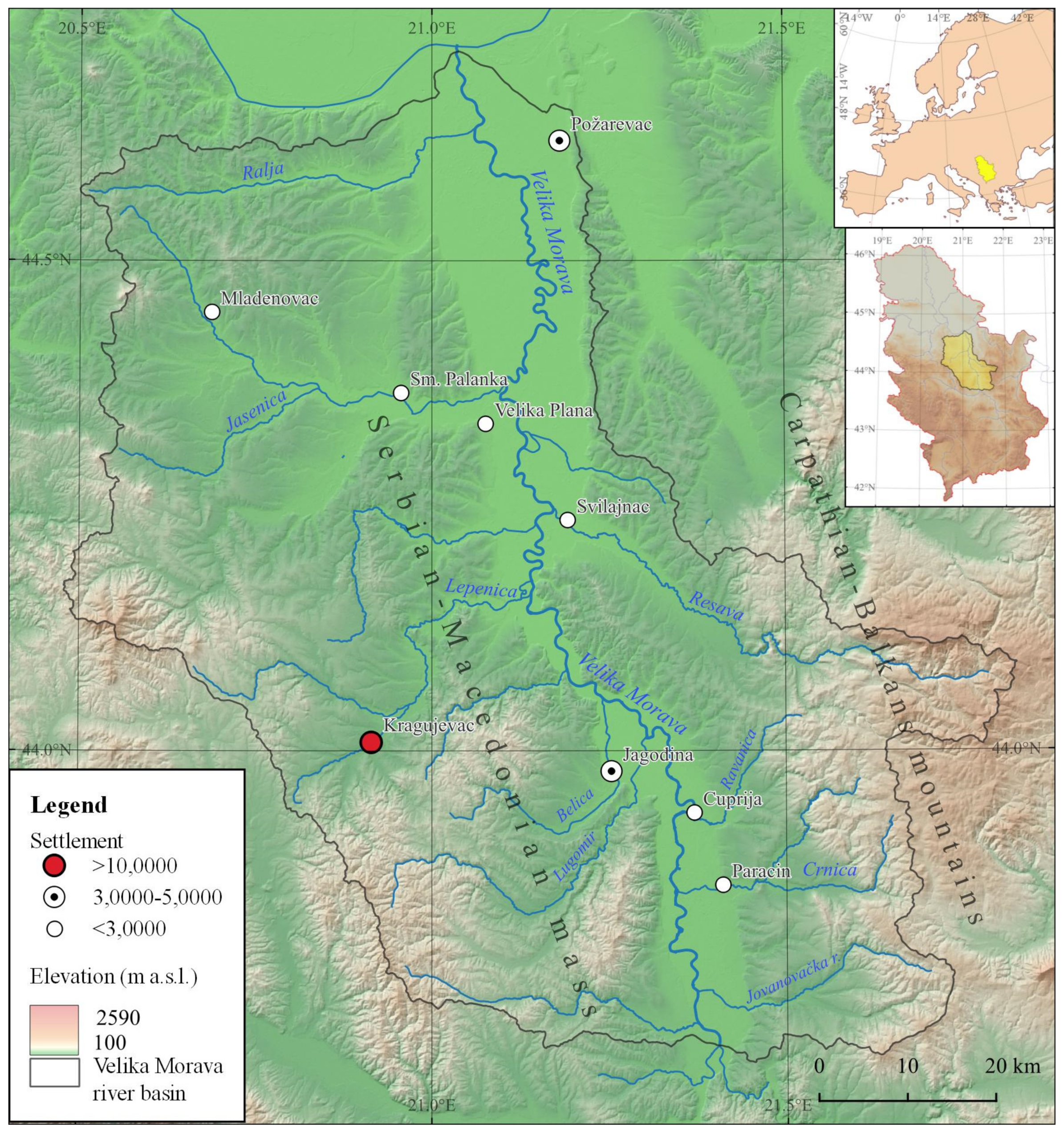
2.1. Study Area
2.2. Erosion Potential Model
2.3. Spatial Autocorrelation Analysis
2.4. Control Variables as Determinants of Changes in Erosion Intensity
3. Results
3.1. Spatio–Temporal Analysis of Changes in Erosion Intensity
3.2. Erosion Intensity Characteristics in Rural Settlements
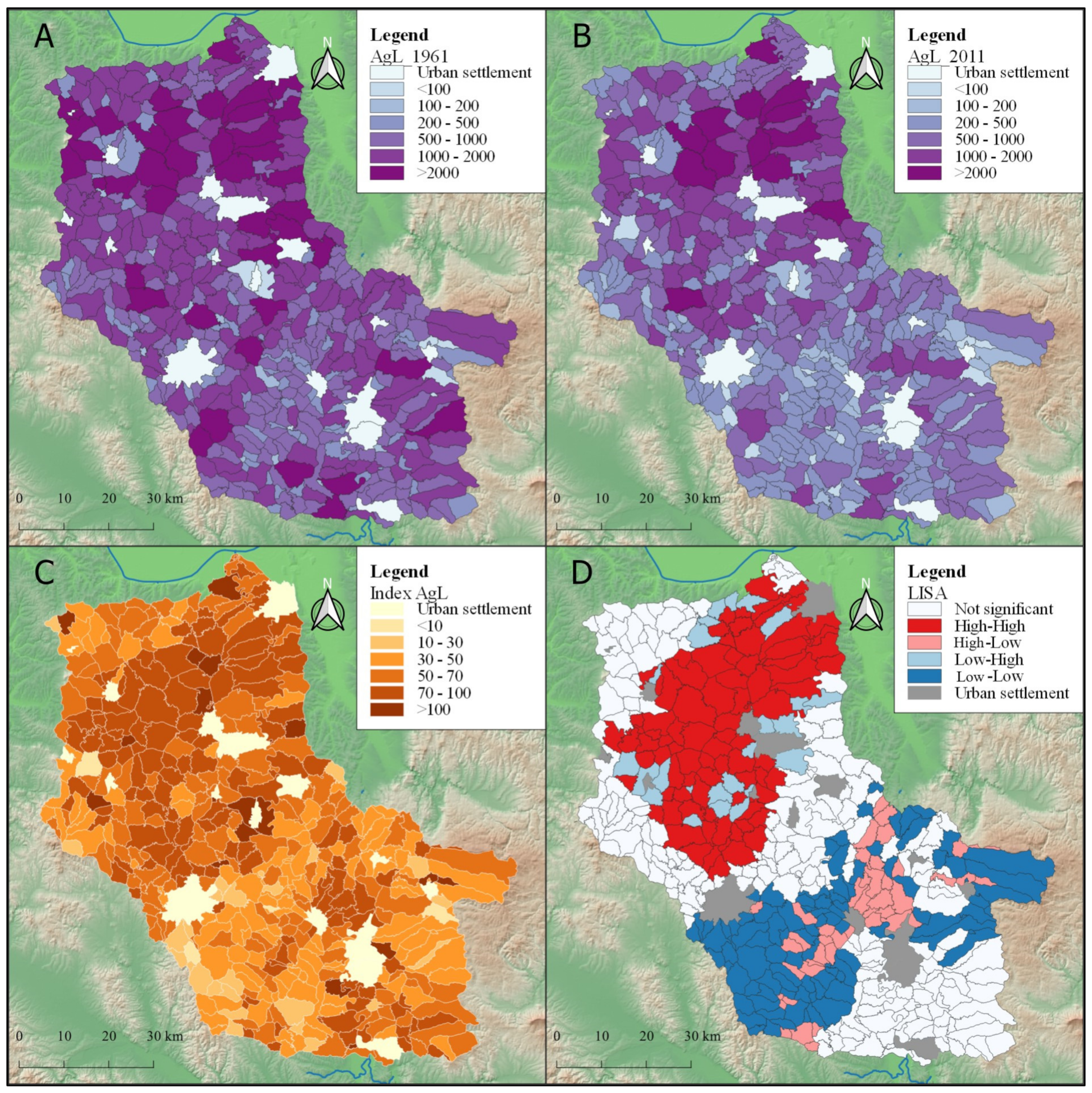
3.3. Agricultural Land Use Characteristics in Rural Settlements
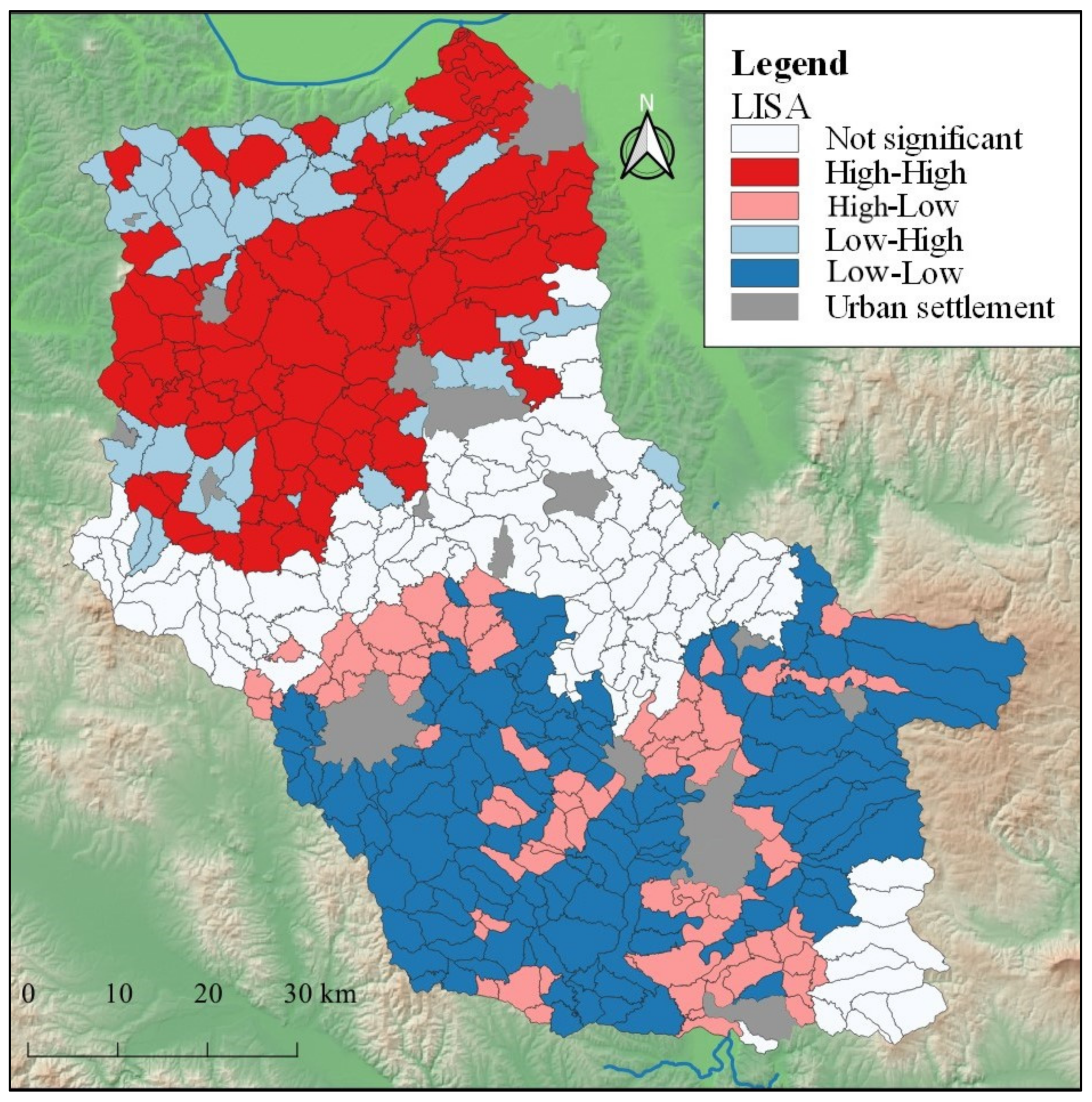
3.4. Spatial Differentiation of Rural Settlements: Impact of Agricultural Land Use Changes on Changes in Erosion Intensity
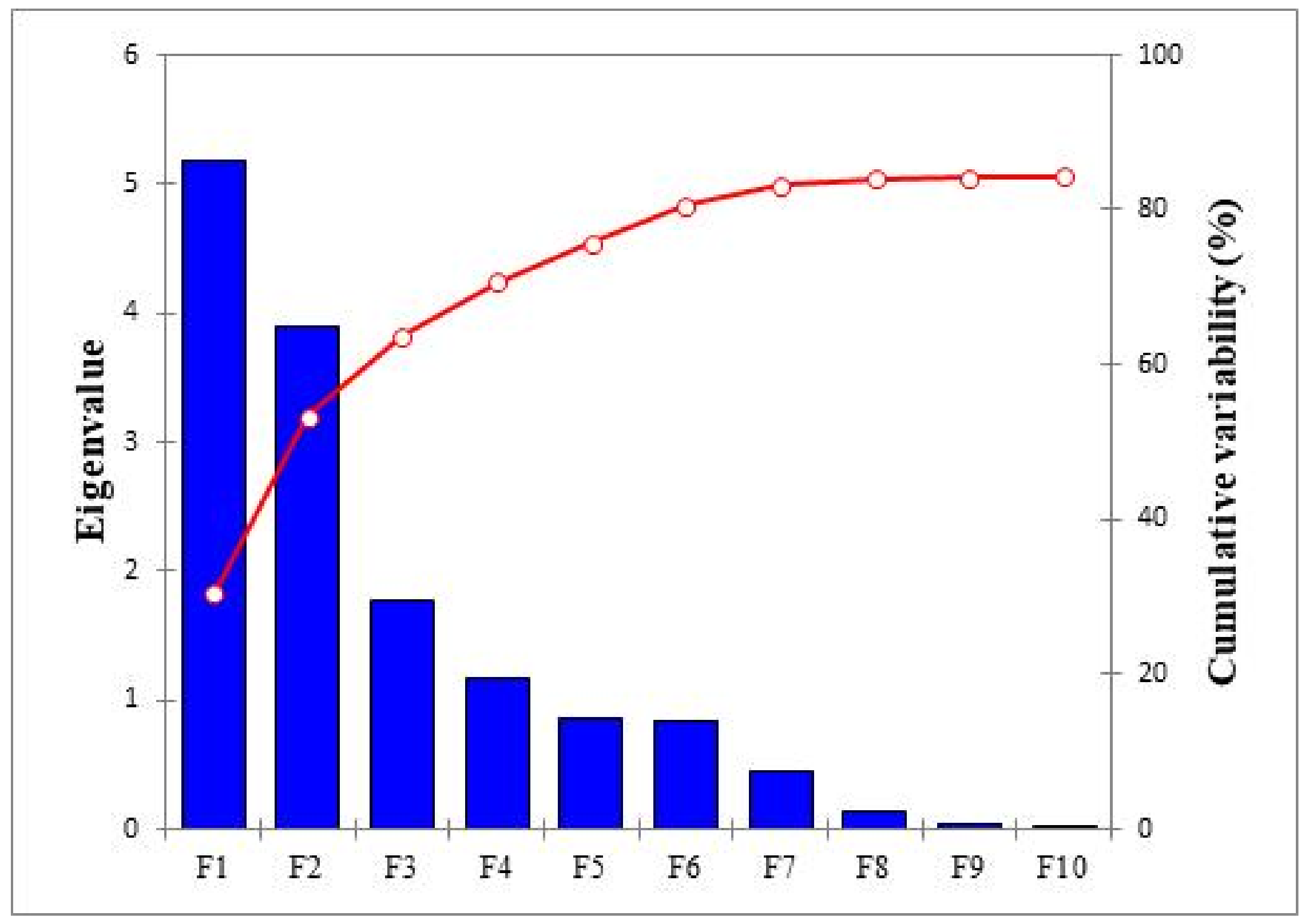
3.5. Geographic Indicators of Changes in Soil Erosion Intensity
4. Discussion
5. Conclusions
Author Contributions
Funding
Institutional Review Board Statement
Informed Consent Statement
Data Availability Statement
Conflicts of Interest
References
- Lal, R. Restoring Soil Quality to Mitigate Soil Degradation. Sustainability 2015, 7, 5875–5895. [Google Scholar] [CrossRef] [Green Version]
- Amundson, R.; Berhe, A.A.; Hopmans, J.W.; Olson, C.; Sztein, A.E.; Sparks, D.L. Soil and human security in the 21st century. Science 2015, 348, 1261071. [Google Scholar] [CrossRef] [PubMed] [Green Version]
- Borrelli, P.; Robinson, D.A.; Panagos, P.; Lugato, E.; Yang, J.E.; Alewell, C.; Wuepper, D.; Montanarella, L.; Ballabio, C. Land use and climate change impacts on global soil erosion by water (2015–2070). Proc. Natl. Acad. Sci. USA 2020, 117, 21994–22001. [Google Scholar] [CrossRef] [PubMed]
- Kucher, A.; Kucher, L.; Sysoieva, I.; Pohrishchuk, B. Economics of soil erosion: Case study of Ukraine. Agric. Econ. 2021, 7, 27–41. [Google Scholar] [CrossRef]
- Di Bene, C.; Francaviglia, R.; Farina, R.; Álvaro-Fuentes, J.; Zornoza, R. Agricultural Diversification. Agriculture 2022, 12, 369. [Google Scholar] [CrossRef]
- Keesstra, S.D.; Bouma, J.; Wallinga, J.; Tittonell, P.; Smith, P.; Cerdà, A.; Montanarella, L.; Quinton, J.; Pachepsky, Y.; Van der Puten, W.; et al. The significance of soils and soil science towards realization of the United Nations Sustainable Development Goals. Soil 2016, 2, 111–128. [Google Scholar] [CrossRef] [Green Version]
- Verheijen, F.G.; Jones, R.J.; Rickson, R.J.; Smith, C.J. Tolerable versus actual soil erosion rates in Europe. Earth Sci. Rev. 2009, 94, 23–38. [Google Scholar] [CrossRef] [Green Version]
- Alewell, C.; Borrelli, P.; Meusburger, K.; Panagos, P. Using the USLE: Chances, challenges and limitations of soil erosion modelling. Int. Soil Water Conserv. Res. 2019, 7, 203–225. [Google Scholar] [CrossRef]
- Petlušová, V.; Petluš, P.; Ševčík, M.; Hreško, J. The Importance of Environmental Factors for the Development of Water Erosion of Soil in Agricultural Land: The Southern Part of Hronská Pahorkatina Hill Land, Slovakia. Agronomy 2021, 11, 1234. [Google Scholar] [CrossRef]
- Tripolskaja, L.; Kazlauskaite-Jadzevice, A.; Baksiene, E.; Razukas, A. Changes in Organic Carbon in Mineral Topsoil of a Formerly Cultivated Arenosol under Different Land Uses in Lithuania. Agriculture 2022, 12, 488. [Google Scholar] [CrossRef]
- Oldeman, L.R. Global Extent of Soil Degradation; Bi-Annual Report 1991–1992/ISRIC; ISRIC: Wageningen, The Netherlands, 1992; pp. 19–36. [Google Scholar]
- Borrelli, P.; Alewell, C.; Alvarez, P.; Anache, J.; Baartman, J.; Ballabio, C.; Bezak, N.; Biddoccu, M.; Cerda, A.; Chalise, D.; et al. Soil erosion modelling: A global review and statistical analysis. Sci. Total Environ. 2021, 780, 146494. [Google Scholar] [CrossRef]
- Pepin, E.; Guyot, J.L.; Armijos, E.; Bazan, H.; Fraizy, P.; Moquet, J.S.; Noriega, L.; Lavado, W.; Pombosa, R.; Vauchel, P. Climatic control on eastern Andean denudation rates (Central Cordillera from Ecuador to Bolivia). J. S. Am. Earth Sci. 2013, 44, 85–93. [Google Scholar] [CrossRef]
- Padonou, E.A.; Anne, M.L.; Yvonne, B.; Rodrigue, I.; Brice, S. Mapping changes in land use/land cover and prediction of future extension of bowé in Benin, West Africa. Land Use Policy 2017, 69, 85–92. [Google Scholar] [CrossRef]
- Tadesse, L.; Suryabhagavan, K.V.; Sridhar, G.; Legesse, G. Land use and land cover changes and Soil erosion in Yezat Watershed, North Western Ethiopia. Int. Soil Water Conserv. Res. 2017, 5, 85–94. [Google Scholar] [CrossRef] [Green Version]
- Tsegaye, B. Effect of land use and land cover changes on soil erosion in Ethiopia. Int. J. Agric. Sci. 2019, 5, 26–34. [Google Scholar] [CrossRef] [Green Version]
- Kogo, B.K.; Kumar, L.; Koech, R. Impact of land use/cover changes on soil erosion in western Kenya. Sustainability 2020, 12, 9740. [Google Scholar] [CrossRef]
- Negese, A. Impacts of land use and land cover change on soil erosion and hydrological responses in Ethiopia. Appl. Environ. Soil Sci. 2021, 2021, 6669438. [Google Scholar] [CrossRef]
- Milazzo, F.; Fernández, P.; Peña, A.; Vanwalleghem, T. The resilience of soil erosion rates under historical land use change in agroecosystems of Southern Spain. Sci. Total Environ. 2022, 822, 153672. [Google Scholar] [CrossRef]
- Abdelsamie, E.A.; Abdellatif, M.A.; Hassan, F.O.; El Baroudy, A.A.; Mohamed, E.S.; Kucher, D.E.; Shokr, M.S. Integration of RUSLE Model, Remote Sensing and GIS Techniques for Assessing Soil Erosion Hazards in Arid Zones. Agriculture 2023, 13, 35. [Google Scholar] [CrossRef]
- Erskine, W.D.; Mahmoudzadeh, A.H.M.A.D.; Myers, C. Land use effects on sediment yields and soil loss rates in small basins of Triassic sandstone near Sydney, NSW, Australia. Catena 2002, 49, 271–287. [Google Scholar] [CrossRef]
- Leh, M.; Bajwa, S.; Chaubey, I. Impact of land use change on erosion risk: An integrated remote sensing, geographic information system and modeling methodology. Land Degrad. Dev. 2013, 24, 409–421. [Google Scholar] [CrossRef]
- Panagos, P.; Borrelli, P.; Meusburger, K.; Van Der Zanden, E.H.; Poesen, J.; Alewell, C. Modelling the effect of support practices (P-factor) on the reduction of soil erosion by water at European scale. Environ Sci. Policy 2015, 51, 23–34. [Google Scholar] [CrossRef]
- Latocha, A.; Szymanowski, M.; Jeziorska, J.; Stec, M.; Roszczewska, M. Effects of land abandonment and climate change on soil erosion—An example from depopulated agricultural lands in the Sudetes Mts., SW Poland. Catena 2016, 145, 128–141. [Google Scholar] [CrossRef]
- Özşahin, E.; Eroğlu, İ. Soil Erosion Risk Assessment due to Land Use/Land Cover Changes (LULCC) in Bulgaria from 1990 to 2015. Alinteri J. Agric. Sci. 2019, 34, 1–8. [Google Scholar] [CrossRef] [Green Version]
- Seeger, M.; Rodrigo-Comino, J.; Iserloh, T.; Brings, C.; Ries, J.B. Dynamics of runoff and soil erosion on abandoned steep vineyards in the Mosel Area, Germany. Water 2019, 11, 2596. [Google Scholar] [CrossRef] [Green Version]
- Niacsu, L.; Bucur, D.; Ionita, I.; Codru, I.C. Soil conservation measures on degraded land in the Hilly Region of Eastern Romania: A case study from Puriceni-Bahnari Catchment. Water 2022, 14, 525. [Google Scholar] [CrossRef]
- Vanwalleghem, T.; Gómez, J.A.; Amate, J.I.; De Molina, M.G.; Vanderlinden, K.; Guzmán, G.; Laguna, A.; Giráldez, J.V. Impact of historical land use and soil management change on soil erosion and agricultural sustainability during the Anthropocene. Anthropocene 2017, 17, 13–29. [Google Scholar] [CrossRef]
- Panagos, P.; Ballabio, C.; Himics, M.; Scarpa, S.; Matthews, F.; Bogonos, M.; Poeson, J.; Borrelli, P. Projections of soil loss by water erosion in Europe by 2050. Environ. Sci. Policy 2021, 124, 380–392. [Google Scholar] [CrossRef]
- Foley, J. Living by the lessons of the planet. Science 2017, 356, 251–252. [Google Scholar] [CrossRef]
- Wang, L.; Lyons, J.; Kanehl, P. Impacts of urbanization on stream habitat and fish across multiple spatial scales. Environ. Manag. 2001, 28, 255–266. [Google Scholar] [CrossRef]
- Falcucci, A.; Maiorano, L.; Boitani, L. Changes in land–use/land–cover patterns in Italy and their implications for biodiversity conservation. Landsc. Ecol. 2007, 22, 617–631. [Google Scholar] [CrossRef]
- Molotoks, A.; Smith, P.; Dawson, T.P. Impacts of land use, population, and climate change on global food security. Food Energy Secur. 2021, 10, e261. [Google Scholar] [CrossRef]
- Soranno, P.A.; Hubler, S.L.; Carpenter, S.R.; Lathrop, R.C. Phosphorus loads to surface waters: A simple model to account for spatial pattern of land use. Ecol. Appl. 1996, 6, 865–878. [Google Scholar] [CrossRef]
- Muller, D.; Kuemmerle, T.; Rusu, M.; Griffiths, P. Lost in Transition: Determinants of post-socialist Cropland Abandonment in Romania. J. Land Use Sci. 2009, 4, 109–129. [Google Scholar] [CrossRef]
- Griffiths, P.; Müller, D.; Kuemmerle, T.; Hostert, P. Agricultural Land Change in the Carpathian Ecoregion after the Breakdown of Socialism and Expansion of the European Union. Environ. Res. Lett. 2013, 8, 045024. [Google Scholar] [CrossRef]
- Kuškova, P.G. A Case Study of the Czech Agriculture since 1918 in a Socio-Metabolic Perspective– from Land Reform through Nationalisation to Privatisation. Land Use Policy 2013, 30, 592–603. [Google Scholar] [CrossRef]
- Pasakarnis, G.; Morley, D.; Maliene, V. Rural Development and Challenges Establishing Sustainable Land Use in Eastern European Countries. Land Use Policy 2013, 30, 703–710. [Google Scholar] [CrossRef]
- Prishchepov, A.V.; Müller, D.; Dubinin, M.; Baumann, M.; Radeloff, V.C. Determinants of Agricultural Land Abandonment in post-Soviet European Russia. Land Use Policy 2013, 30, 873–884. [Google Scholar] [CrossRef] [Green Version]
- Pazúr, R.; Lieskovský, J.; Feranec, J.; Oťaheľ, J. Spatial Determinants of Abandonment of Large-Scale Arable Lands and Managed Grasslands in Slovakia during the Periods of post-socialist Transition and European Union Accession. Appl. Geogr. 2014, 54, 118–128. [Google Scholar] [CrossRef]
- Gusarov, A.V. Land–Use/Cover Changes and Their Effect on Soil Erosion and River Suspended Sediment Load in Different Landscape Zones of European Russia during 1970–2017. Water 2021, 13, 1631. [Google Scholar] [CrossRef]
- Bogdanov, N.; Vasiljević, Z. Role of agriculture and multifunctional rural development in Serbia. Appl. Stud. Agribus. Commer. 2011, 5, 47–55. [Google Scholar] [CrossRef]
- Manojlović, S.; Sibinović, M.; Srejić, T.; Novković, I.; Milošević, M.V.; Gatarić, D.; Carević, I.; Batoćanin, N. Factors Controlling the Change of Soil Erosion Intensity in Mountain Watersheds in Serbia. Front. Environ. Sci. 2022, 10, 88901. [Google Scholar] [CrossRef]
- Manojlović, S.; Antić, M.; Šantić, D.; Sibinović, M.; Carević, I.; Srejić, T. Anthropogenic Impact on Erosion Intensity: Case Study of Rural Areas of Pirot and Dimitrovgrad Municipalities, Serbia. Sustainability 2018, 10, 826. [Google Scholar] [CrossRef] [Green Version]
- Manojlović, S.; Sibinović, M.; Srejić, T.; Hadud, A.; Sabri, I. Agriculture land use change and demographic change in response to decline suspended sediment in Južna Morava River basin (Serbia). Sustainability 2021, 13, 3130. [Google Scholar] [CrossRef]
- Menković, L.; Košćal, M.; Milivojević, M.; Đokić, M. Morphostructure relations on the territory of the Republic of Serbia. Bull. Serb. Geogr. Soc. 2018, 98, 1–28. [Google Scholar] [CrossRef] [Green Version]
- Manojlović, S.; Manojlović, P.; Đokić, M. Dynamics of suspended sediment load in the Morava River (Serbia) in the period 1967-2007. Rev. Geomorfol. 2016, 18, 47–58. [Google Scholar] [CrossRef]
- Milovanović, B.; Ducić, V.; Radovanović, M.; Milivojević, M. Climate regionalization of Serbia according to Köppen climate classification. J. Geograph. Inst. “Jovan Cvijić” SASA 2017, 67, 103–114. [Google Scholar] [CrossRef] [Green Version]
- Blagojević, B.; Langović, M.; Novković, I.; Dragićević, S.; Živković, N. Water Resources of Serbia and Its Utilization. In Water Resources Management in Balkan Countries; Springer: Berlin/Heidelberg, Germany, 2020; pp. 213–247. [Google Scholar]
- Bačević, N.R.; Milentijević, N.M.; Valjarević, A.; Gicić, A.; Kićović, D.; Radaković, M.G.; Nikolić, M.; Pantelić, M. Spatiotemporal variability of air temperatures in Central Serbia from 1949 to 2018. Időjárás/Q. J. Hung. Meteorol. Serv. 2021, 125, 229–253. [Google Scholar] [CrossRef]
- Milovanović, B.; Stanojević, G.; Radovanović, M. Climate of Serbia. In The Geography of Serbia; Springer: Berlin/Heidelberg, Germany, 2022; pp. 57–68. [Google Scholar]
- Radaković, M.G.; Tošić, I.; Bačević, N.; Mladjan, D.; Gavrilov, M.B.; Marković, S.B. The analysis of aridity in Central Serbia from 1949 to 2015. Theor. Appl. Climatol. 2018, 133, 887–898. [Google Scholar] [CrossRef]
- Gocić, M.; Trajković, S. Spatio-temporal patterns of precipitation in Serbia. Theor. Appl. Climatol. 2014, 117, 419–431. [Google Scholar] [CrossRef]
- Valjarević, A.; Morar, C.; Živković, J.; Niemets, L.; Kićović, D.; Golijanin, J.; Gocić, M.; Martić Bursać, N.; Stričević, L.J.; Žiberna, I.; et al. Long term monitoring and connection between topography and cloud cover distribution in Serbia. Atmosphere 2021, 12, 964. [Google Scholar] [CrossRef]
- Pešić, A. Water regime and discharges trends of the rivers in the Šumadija region (Serbia). In Proceedings of the International Scientific Symposium “New trends in geography”, Ohrid, North Macedonia, 3–4 October 2019; pp. 3–13. [Google Scholar]
- Petrović, A. Torrential Floods in Serbia; Special Issues 73; Serbian Geographical Society: Belgrade, Serbia, 2021. [Google Scholar]
- Ristić, R.; Kostadinov, S.; Abolmasov, B.; Dragićević, S.; Trivan, G.; Radić, B.; Trifunović, M.; Radosavljević, Z. Torrential floods and town and country planning in Serbia. Nat. Hazards Earth Syst. Sci. 2012, 12, 23–35. [Google Scholar] [CrossRef]
- Urošev, M.; Milanović Pešić, A.; Kovačević–Majkić, J.; Štrbac, D. Hydrological Characteristics of Serbia. In The Geography of Serbia, Nature, People, Economy; Manić, E., Nikitović, V., Đurović, P., Eds.; Springer: Berlin/Heidelberg, Germany, 2022; pp. 69–84. [Google Scholar]
- Gavrilović, L.; Milanović Pešić, A.; Urošev, M. A Hydrological Analysis of the Greatest Floods in Serbia in the 1960–2010 Period. Carpathian J. Earth Environ. Sci. 2012, 7, 107–116. [Google Scholar]
- Dragićević, S.; Filipović, D.; Kostadinov, S.; Ristić, R.; Novković, I.; Živković, N.; Anđelković, G.; Abolmasov, B.; Šećerov, V.; Đurdjic, S. Natural hazard assessment for land-use planning in Serbia. Int. J. Environ. Res. 2011, 5, 371–380. [Google Scholar]
- Novković, I.; Dragićević, S.; Đurović, M. Geohazard and Geoheritage. In The Geography of Serbia, Nature, People, Economy; Manić, E., Nikitović, V., Đurović, P., Eds.; Springer: Berlin/Heidelberg, Germany, 2022; pp. 119–131. [Google Scholar]
- FAO Soil Portal (World Reference Base). Available online: https://www.fao.org/soils-portal/data-hub/soil-classification/world-reference-base/en/ (accessed on 20 March 2023).
- Statistical Office of the Republic of Serbia 1961–2012. Available online: http://www.stat.gov.rs (accessed on 10 September 2022).
- Gavrilović, S. Engineering of Torrential Flows and Erosion; Izgradnja: Belgrad, Serbia, 1972; 272p. [Google Scholar]
- Zorn, M.; Komac, B. Response of Soil Erosion to Land Use Change with Particular Reference to the Last 200 Years (Julian Alps, Western Slovenia). In Proceedings of the IAG Regional Conference on Geomorphology: Landslides, Floods and Global Environmental Change in Mountain Regions, Brasov, Romania, 15–25 September 2008; pp. 39–47. [Google Scholar]
- Tošić, R.; Dragićević, S.; Lovrić, N. Assessment of soil erosion and sediment yield changes using erosion potential model–case study: Republic of Srpska (BiH). Carpathian J. Earth Environ. Sci. 2012, 7, 147–154. [Google Scholar]
- Blinkov, I.; Marinov, I.; Kostadinov, S. Comparison of Erosion and Erosion Control Works in Macedonia, Serbia and Bulgaria. Int. Soil Water Conserv. Res. 2013, 1, 15–28. [Google Scholar] [CrossRef] [Green Version]
- Efthimiou, N.; Lykoudi, E.; Panagoulia, D.; Karavitis, C. Assessment of Soil Susceptibility to Erosion Using the EPM and RUSLE MODELS: The Case of Venetikos River Catchment. Glob. NEST J. 2016, 18, 164–179. [Google Scholar]
- Manojlović, S.; Antić, M.; Sibinović, M.; Dragićević, S.; Novković, I. Soil erosion response to demographic and land use changes in the Nišava River basin, Serbia. Fresenius Environ. Bull. 2017, 26, 7547–7560. [Google Scholar]
- Dragičević, N.; Karleuša, B.; Ožanić, N. Modification of erosion potential method using climate and land cover parameters. Geomatics, Nat. Hazards Risk. 2018, 9, 1085–1105. [Google Scholar] [CrossRef] [Green Version]
- Lovrić, N.; Tošić, R. Assessment of soil erosion and sediment yield using erosion potential method: Case study–Vrbas River basin (B&H). Bull. Serb. Geogr. Soc. 2018, 98, 1–14. [Google Scholar]
- Blinkov, I.; Kostadinov, S. Applicability of various erosion risk assessment methods for engineering purposes. In Proceedings of the BALWOIS Conference, Ohrid, North Macedonia, 25–29 May 2010. [Google Scholar]
- Bazzoffi, P. Methods for net erosion measurement in watersheds as a tool for the validation of models in central Italy. In Workshop on Soil Erosion and Hillslope Hydrology with Emphasis on Higher Magnitude Events; K.U.: Leuven, Belgium, 1985. [Google Scholar]
- Beyer, P.N. Erosion des Bassins Versant Alpins Suisses par Ruissellement de Surface. Ph.D. Thesis, University of Switzerland, Laussanne, Switzerland, 1998; 438p. [Google Scholar]
- Fanetti, D.; Vezzoli, L. Sediment input and evolution of lacustrine deltas: The Breggia and Greggio rivers case study (Lake Como, Italy). Quat. Int. 2007, 173, 113–124. [Google Scholar] [CrossRef]
- Poggetti, E.; Cencetti, C.; De Rosa, P.; Fredduzzi, A.; Rivelli, F.R. Sediment Supply and Hydrogeological Hazard in the Quebrada De Humahuaca (Province of Jujuy, Northwestern Argentina)—Rio Huasamayo and Tilcara Area. Geosciences 2019, 9, 483. [Google Scholar] [CrossRef] [Green Version]
- Ouallali, A.; Aassoumi, H.; Moukhchane, M.; Moumou, A.; Houssni, M.; Spalevic, V.; Keesstra, S. Sediment mobilization study on Cretaceous, Tertiary and Quaternary lithological formations of an external Rif catchment, Morocco. Hydrol. Sci. J. 2020, 65, 1568–1582. [Google Scholar] [CrossRef]
- Mohammadi, M.; Khaledi Darvishan, A.; Spalević, V.; Dudić, B.; Billi, P. Analysis of the Impact of Land Use Changes on Soil Erosion Intensity and Sediment Yield Using the IntErO Model in the Talar Watershed of Iran. Water 2021, 13, 881. [Google Scholar] [CrossRef]
- Luković, J.; Bajat, B.; Blagojević, D.; Kilibarda, M. Spatial pattern of recent rainfall trends in Serbia (1961–2009). Reg. Environ. Chang. 2014, 14, 1789–1799. [Google Scholar] [CrossRef]
- Solaimani, K.; Modallaldoust, S.; Lotfi, S. Investigation of land use changes on soil erosion process using geographical information system. Int. J. Environ. Sci. Technol. 2009, 6, 415–424. [Google Scholar] [CrossRef] [Green Version]
- Sharma, A.; Tiwari, K.N.; Bhadoria, P.B. Effect of land use land cover change on soil erosion potential in an agricultural watershed. Environ. Monit. Assess. 2011, 173, 789–801. [Google Scholar] [CrossRef]
- Serpa, D.; Nunes, J.P.; Santos, J.; Sampaio, E.; Jacinto, R.; Veiga, S.; Lima, J.C.; Moreira, M.; Corte–Real, J.; Keizer, J.J. Impacts of climate and land use changes on the hydrological and erosion processes of two contrasting Mediterranean catchments. Sci. Total Environ. 2015, 538, 64–77. [Google Scholar] [CrossRef] [Green Version]
- Perović, V.; Kadović, R.; Ðurdević, V.; Braunović, S.; Čakmak, D.; Mitrović, M.; Pavlović, P. Effects of changes in climate and land use on soil erosion: Case study of the Vranjska Valley, Serbia. Reg. Environ. Chang. 2019, 19, 1035–1046. [Google Scholar] [CrossRef]
- Uddin, K.; Abdul Matin, M.; Maharjan, S. Assessment of land cover change and its impact on changes in soil erosion risk in Nepal. Sustainability 2018, 10, 4715. [Google Scholar] [CrossRef] [Green Version]
- Devátý, J.; Dostál, T.; Hösl, R.; Krása, J.; Strauss, P. Effects of historical land use and land pattern changes on soil erosion–Case studies from Lower Austria and Central Bohemia. Land Use Policy 2019, 82, 674–685. [Google Scholar] [CrossRef]
- Moisa, M.B.; Negash, D.A.; Merga, B.B.; Gemeda, D.O. Impact of land-use and land-cover change on soil erosion using the RUSLE model and the geographic information system: A case of Temeji watershed, Western Ethiopia. J. Water Clim. Chang. 2021, 12, 3404–3420. [Google Scholar] [CrossRef]
- Anselin, L. Local indicators of spatial association-LISA. Geogr. Anal. 1995, 27, 93–115. [Google Scholar] [CrossRef]
- O’Sullivan, D.; Unwin, D. Geographic Information Analysis; John Wiley & Sons: Hoboken, NJ, USA, 2010; 432p. [Google Scholar]
- Anselin, L.; Syabri, I.; Smirnov, O. Visualizing Multivariate Spatial Correlation with Dynamically Linked Windows. In New Tools for Spatial Data Analysis: Proceedings of the Specialist Meeting; Anselin, L., Rey, S., Eds.; Center for Spatially Integrated Social Science (CSISS), University of California: Santa Barbara, CA, USA, 2002. [Google Scholar]
- Anselin, L.; Syabri, I.; Youngihn, K. GeoDa: An Introduction to Spatial Data Analysis. Geogr. Anal. 2006, 38, 5–22. [Google Scholar] [CrossRef]
- Lazarević, R. The Erosion Map of Serbia. Scale 1:500000; Institute of Forestry: Belgrade, Serbia, 1983. [Google Scholar]
- Copernicus Land Monitoring Service (2012). CORINE Land Cover (CLC). Available online: https://land.copernicus.eu/pan-european/corine-land-cover/clc2012 (accessed on 15 September 2021).
- Novković, I. Natural Conditions as Determinants of Geohazards on the Example of Ljig, Jošanička and Vranjskobanjska River Basins. Ph.D. Thesis, University of Belgrade, Faculty of Geography, Belgrade, Serbia, 2016. [Google Scholar]
- Kostadinov, S.; Dragićević, S.; Stefanović, T.; Novković, I.; Petrović, A.M. Torrential flood prevention in the Kolubara River basin. J. Mt. Sci. 2017, 14, 2230–2245. [Google Scholar] [CrossRef]
- Durlević, U.; Momčilović, A.; Ćurić, V.; Dragojević, M. Gis application in analysis of erosion intensity in the Vlasina River Basin. Bull. Serb. Geogr. Soc. 2019, 99, 17–36. [Google Scholar] [CrossRef]
- Durlević, U.; Novković, I.; Lukić, T.; Valjarević, A.; Samardžić, I.; Krstić, F.; Batoćanin, N.; Mijatov, M.; Ćurić, V. Multihazard susceptibility assessment: A case study–Municipality of Štrpce (Southern Serbia). Open Geosci. 2021, 13, 1414–1431. [Google Scholar] [CrossRef]
- Dragićević, S.; Kostadinov, S.; Novković, I.; Momirović, N.; Langović, M.; Stefanović, T.; Radović, M.; Tošić, R. Assessment of Soil Erosion and Torrential Flood Susceptibility: Case Study—Timok River Basin, Serbia. In The Lower Danube River: Hydro-Environmental Issues and Sustainability; Negm, A., Zaharia, L., Ioana–Toroimac, G., Eds.; Springer: Berlin/Heidelberg, Germany, 2022; pp. 357–380. [Google Scholar]
- Krstić, F.; Paunović, S. Changes in Soil Erosion Intensity in Jablanica Region; Collection of Papers; University of Belgrade, Faculty of Geography: Belgrade, Serbia, 2022; pp. 83–93. [Google Scholar] [CrossRef]
- Copernicus Land Monitoring Service (2020). Imagery and Reference Data, EU-DEM v1.1. Available online: https://land.copernicus.eu/imagery-in-situ/eudem/eu-dem-v1.1 (accessed on 25 September 2021).
- Geološki zavod Srbije. Basic Geological Map of Former Yugoslavia 1:100 000; Federal Geological Survey: Belgrade, Serbia, 1978. [Google Scholar]
- R Core Team. R: A Language and Environment for Statistical Computing. R Foundation for Statistical Computing; R Core Team: Vienna, Austria, 2012; Available online: http://www.R-project.org/ (accessed on 7 March 2022)ISBN 3-900051-07-0.
- Wuttichaikitcharoen, P.; Babel, M.S. Principal component and multiple regression analyses for the estimation of suspended sediment yield in ungauged basins of northern Thailand. Water 2014, 6, 2412–2435. [Google Scholar] [CrossRef] [Green Version]
- Sibinović, M. Typology of Agriculture in Conditions of Transitional Crisis: The Case of the Belgrade Region; Collection of Papers; University of Belgrade, Faculty of Geography: Belgrade, Serbia, 2015; pp. 81–118. [Google Scholar]
- Matejka, K. Multivariate Analysis for Assessment of the Tree Populations Based on Dendrometric Data with an Example of Similarity Among Norway spruce Subpopulations. J. For. Sci. 2017, 63, 449–456. [Google Scholar] [CrossRef] [Green Version]
- Mizuta, K.; Grunwald, S.; Phillips, M.A. New Soil Index Development and Integration with Econometric Theory. Soil Sci. Soc. Am. J. 2018, 82, 1017–1032. [Google Scholar] [CrossRef] [Green Version]
- Kaiser, H. An index of factorial simplicity. Psychometrika 1974, 39, 31–36. [Google Scholar] [CrossRef]
- Hair, J.F.; Black, B.; Babin, B.; Anderson, R.E.; Tatham, R.L. Multivariate Data Analysis, 6th ed.; Pearson Prentice Hall: Upper Saddle River, NJ, USA, 2006; pp. 1–816. [Google Scholar]
- Williams, B.; Onsman, A.; Brett, A.; Brown, T. Exploratory factor analysis: A five-step guide for novices. Australas. J. Paramed. 2012, 8, 1–13. [Google Scholar] [CrossRef] [Green Version]
- Ševarlić, M.; Tomić, D. Serbian agriculture in crisis condition. JUMTO 2009, 14, 157–164. [Google Scholar]
- Sibinović, M. How Did Agricultural Patterns Change in Serbia After the Fall of Yugoslavia? Geogr. Teach. 2018, 15, 33–35. [Google Scholar] [CrossRef]
- Gatarić, D. The daily urban system of the Knjaževac. In Region of Knjaževac-Potential, Current State and Prospects; Sibinović, M., Stojadinović, V., Popović Nikolić, D., Eds.; National library Njegoš: Knjaževac, Serbia, 2019; pp. 78–85. [Google Scholar]
- Sibinović, M. Structural Changes and Spatial Differentiation of Agriculture in Rural Settlements of Belgrade Region. Ph.D. Thesis, University of Belgrade, Faculty of Geography, Belgrade, Serbia, 2014. [Google Scholar]
- Bański, J. Agriculture of Central Europe in the Period of Economic Transformation. Rural Stud. 2008, 15, 9–22. [Google Scholar]
- Sibinović, M.; Winkler, A.; Grčić, M. Agriculture in a transitional crisis period: Crop production in the administrative region of Belgrade from 1991 to 2002. Mitt. Osterr. Geogr. Ges. 2014, 156, 293–310. [Google Scholar] [CrossRef] [Green Version]
- Kostov, P.; Lingard, J. Subsistence agriculture in transition economies: Its roles and determinants. J. Agric. Econ. 2004, 55, 565–579. [Google Scholar] [CrossRef]
- Mc Donagh, J. Rural Geography I: Changing Expectations and Contradictions in the Rural. Prog. Hum. Geogr. 2012, 37, 712–720. [Google Scholar] [CrossRef]
- Arsenović, D.; Nikitović, V. Demographic Profile of Serbia at the Turn of the Millennia. In The Geography of Serbia, Nature, People, Economy; Manić, E., Nikitović, V., Đurović, P., Eds.; Springer: Berlin/Heidelberg, Germany, 2022; pp. 135–141. [Google Scholar]
- Todorović, M. The Base of Typology and Regionalization of Agriculture of Serbia; Serbian Geographical Society: Belgrade, Serbia, 2002; pp. 1–164. [Google Scholar]
- Čobeljić, N. Položaj Poljoprivrede u Procesu Privrednog Razvoja, Prilozi sa Skupa Razvojni i Sistemski Problemi Poljoprivrede Jugoslavije; Ekonomski Zbornik: Beograd, Serbia, 1986. [Google Scholar]
- Martinović, M.; Ratkaj, I. Sustainable rural development in Serbia: Towards a quantitative typology of rural areas. Carpathian J. Earth Environ. Sci. 2015, 10, 37–48. [Google Scholar]
- Drobnjaković, M.; Petrović, G.; Karabašević, D.; Vukotić, S.; Mirčetić, V.; Popović, V. Socio–economic transformation of Šumadija district (Serbia). J. Geograph. Inst. “Jovan Cvijić” SASA 2021, 71, 163–180. [Google Scholar] [CrossRef]
- Lukić, V. Migration and Mobility Paterns in Serbia. In The Geography of Serbia, Nature, People, Economy; Manić, E., Nikitović, V., Đurović, P., Eds.; Springer: Berlin/Heidelberg, Germany, 2022; pp. 157–168. [Google Scholar]
- Sibinović, M. Structural changes in the rural planting areas of Belgrade region. Bull. Serb. Geogr. Soc. 2012, 92, 112–132. [Google Scholar] [CrossRef]
- Pagáč Mokrá, A.; Pagáč, J.; Muchová, Z.; Petrovič, F. Analysis of ownership data from consolidated land threatened by water erosion in the Vlára basin, Slovakia. Sustainability 2020, 13, 51. [Google Scholar] [CrossRef]
- Gorgan, M.; Hartvigsen, M. Development of agricultural land markets in countries in Eastern Europe and Central Asia. Land Use Policy 2022, 120, 106257. [Google Scholar] [CrossRef]
- Jordan, P. Development of rural space in post-communist Southeast Europe after 1989: A comparative analysis. Revija Za Geografijo-Geogr. J. 2009, 4, 89–102. [Google Scholar]
- Živanović, Z.; Tošić, B.; Nikolić, T.; Gatarić, D. Urban System in Serbia—The Factor in the Planning of Balanced Regional Development. Sustainability 2019, 11, 4168. [Google Scholar] [CrossRef] [Green Version]
- Gajić, A.; Krunić, N.; Protić, B. Classification of rural areas in Serbia: Framework and implications for spatial planning. Sustainability 2021, 13, 1596. [Google Scholar] [CrossRef]
- Antrop, M.; Van Eetvelde, V. Holistic aspects of suburban landscapes: Visual image interpretation and landscape metrics. Landsc. Urban Plan. 2000, 50, 43–58. [Google Scholar] [CrossRef]
- Golosov, V.; Yermolaev, O.; Litvin, L.; Chizhikova, N.; Kiryukhina, Z.; Safina, G. Influence of climate and land use changes on recent trends of soil erosion rates within the Russian Plain. Land Degrad. Dev. 2018, 29, 2658–2667. [Google Scholar] [CrossRef]
- Mal’tsev, K.A.; Ivanov, M.A.; Sharifullin, A.G.; Golosov, V.N. Changes in the rate of soil loss in river basins within the Southern Part of European Russia. Eurasian Soil Sci. 2019, 52, 718–727. [Google Scholar] [CrossRef]
- Van Rompaey, A.; Govers, G.; Verstraeten, G.; van Oost, K.; Poesen, J. Modelling the geomorphic response to land use changes. In Long Term Hillslope and Fluvial System Modelling–Concepts and Case Studies from the Rhine River Catchment; Lang, A., Dikau, R., Hennnrich, K., Eds.; Springer: Berlin/Heidelberg, Germany, 2003; pp. 73–100. [Google Scholar]
- Gusarov, A.A. The impact of contemporary changes in climate and land use/cover on tendencies in water flow, suspended sediment yield and erosion intensity in the northeastern part of the Don river basin, SW European Russia. Environ. Res. 2019, 175, 468–488. [Google Scholar] [CrossRef]
- Tošić, R.; Lovrić, N.; Dragićević, S. Assesment of the impact of depopulation on soil erosion: Case study Republika Srpska (Bosnia and Herzegovina). Carpathian J. Earth Environ. Sci. 2019, 14, 505–518. [Google Scholar] [CrossRef]
- Kostadinov, S.; Zlatić, M.; Dragićević, S.; Novković, I.; Košanin, O.; Borisavljević, A.; Lakićević, M.; Mlađan, D. Anthropogenic influence on erosion intensity changes in the Rasina river watershed-Central Serbia. Fresenius Environ. Bull. 2014, 23, 254–263. [Google Scholar]
- Gocić, M.; Dragićević, S.; Radivojević, A.; Martić Bursać, N.; Stričević, L.; Đorđević, M. Changes in soil erosion intensity caused by land use and demographic changes in the Jablanica River Basin, Serbia. Agriculture 2020, 10, 345. [Google Scholar] [CrossRef]
- Kostadinov, S.; Braunović, S.; Dragićević, S.; Zlatić, M.; Dragović, N.; Rakonjac, N. Effects of erosion control works: Case study—Grdelica Gorge, the South Morava River (Serbia). Water 2018, 10, 1094. [Google Scholar] [CrossRef] [Green Version]


| Coefficient of Soil Resistance | Y Value |
| Fine sediments and soils without erosion resistance | 0.80–1.00 |
| Sediments, moraines, clay and other rock with little resistance | 0.60–0.80 |
| Weak rock, schistose, stabilized | 0.50–0.60 |
| Rock with moderate erosion resistance | 0.30–0.50 |
| Hard rock, erosion resistant | 0.10–0.30 |
| Coefficient of soil protection | X value |
| Areas without vegetal cover | 0.08–1.00 |
| Damaged pasture and cultivated land | 0.06–0.80 |
| Damaged forest and bushes, pasture | 0.04–0.06 |
| Coniferous forest with little grove, scarce bushes, bushy prairie | 0.20–0.40 |
| Thin forest with grove | 0.05–0.20 |
| Mixed and dense forest | 0.05–0.20 |
| Coefficient of type and extent of erosion | φ value |
| Whole watershed affected by erosion | 0.90–1.00 |
| 50–80% of the catchment area is affected by surface erosion and landslides | 0.80–0.90 |
| Erosion in rivers, gullies and alluvial deposits, karstic erosion | 0.60–0.70 |
| Erosion in waterways on 20–50% of the catchment area | 0.30–0.50 |
| Little erosion on watershed | 0.10–0.20 |
| Erosion Category | Erosion Intensity | Range of Z | Average of Z | Range of W (m3/km2/yr) |
| I | Excessive erosion | >1.01 | 1.25 | >3000 |
| II | Intensive erosion | 0.71–1.00 | 0.85 | 1200–3000 |
| III | Medium erosion | 0.41–0.70 | 0.55 | 800–1200 |
| IV | Weak erosion | 0.21–0.40 | 0.30 | 400–800 |
| V | Very weak erosion | 0.01–0.20 | 0.10 | 100–400 |
| Variables–Abbreviation (Units) | Calculate | |
| Physical–geographical | ||
| Erosion coefficient in 2011 Z2 (–) | Equation (2) | X, Z, φ—Table 1 |
| Mean Altitude Aav (m) | DEM | DEM—Digital Elevation Model |
| Terrain slope I (°) | DEM | DEM—Digital Elevation Model |
| Lithology—sediments of Neogen NSA (%) | NSA = (ANSA/A)∙100 | ANSA—Neogen sediments area A—total area of the settlement |
| Vegetation—Forest cover FC (%) | FC = (AFC/A)∙100 | AFC—forest area in 2011 A—total area of the settlement |
| Agrarian–geographical | ||
| Deagrarization index agricultural land Index AgL (–) | Index AgL = (AgL2/AgL1)∙100 | AgL2—agricultural land (ha) in 2011 AgL1—agricultural land (ha) in 1961 |
| Deagrarization index arable land Index ArL (–) | Index ArL = (ArL2/ArL1)∙100 | ArL2—arable land (ha) in 2011 ArL1—arable land (ha) in 1961 |
| Share of arable land in agricultural land ArLs (%) | ArLs = (ArL/AgL)∙100 | ArL—arable land (ha) in 2011 AgL—agricultural land (ha) in 2011 |
| General agrarian population density GDAgL (rural population/100 ha) | GDAgL = RP/AgL∙100 | RP—rural population in 2011 AgL—agricultural land (100 ha) in 2011 |
| Specific agrarian population density SDArL(rural population/100 ha) | SDArL= RP/ArL∙100 | RP—rural population in 2011 ArL—arable land (100 ha) in 2011 |
| Demographic | ||
| Depopulation index Index RP (–) | Index RP = (RP2/RP1)∙100 | RP2—rural population in 2011 RP1—rural population in 1961 |
| Density rural population DRP (rural population/km2) | DRP = RP/A | RP—rural population in 2011 A—total area of the settlement |
| Vitality index Index V (–) | Index V = (WRP/ORP)∙100 | WRP—economically active rural population in 2011 ORP—rural population older than 65 yr in 2011 |
| The average age of the rural population RPav (years) | Age and Sex, data by settlements 2011 | |
| Old rural population ORP (%) | ORP = (ORP/RP)∙100 | ORP—rural population older than 65 yr in 2011 RP—rural population in 2011 |
| Household index Index H (–) | Index H = (H2/H1)∙100 | H2—total number of households in 2011 H1—total number of households in 1961 |
| Household index size Index Hs (–) | Index Hs = (Hs2/Hs1)∙100 | Hs2—average household size in 2011 Hs1—average household size in 1961 |
| Erosion Category | Erosion Intensity | F (km2) 1971 | F (%) 1971 | F (km2) 2011 | F (%) 2011 |
| I | Excessive erosion | 310.3 | 4.6 | 4.0 | 0.1 |
| II | Intensive erosion | 2111.8 | 31.4 | 1094.0 | 16.2 |
| III | Medium erosion | 2093.2 | 31.1 | 2580.9 | 38.3 |
| IV | Weak erosion | 1060.1 | 15.7 | 1021.1 | 15.2 |
| V | Very weak erosion | 1159.2 | 17.2 | 2034.5 | 30.2 |
| Z2 | Aav | I | NSA | FC | Index AgL | Index ArL | ArLs | GDAgL | SDArL | Index RP | DRP | Index V | RPav | ORP | Index H | Index Hs | |
| Z2 | 1 | ||||||||||||||||
| Aav | −0.379 | 1 | |||||||||||||||
| I | −0.445 | 0.893 | 1 | ||||||||||||||
| NSA | 0.254 | −0.856 | −0.837 | 1 | |||||||||||||
| FC | −0.405 | 0.010 | 0.174 | 0.063 | 1 | ||||||||||||
| Index AgL | 0.091 | 0.028 | −0.026 | 0.034 | −0.272 | 1 | |||||||||||
| Index ArL | 0.473 | −0.236 | −0.288 | 0.235 | −0.182 | 0.711 | 1 | ||||||||||
| ArLs | 0.583 | −0.692 | −0.705 | 0.643 | 0.042 | 0.054 | 0.596 | 1 | |||||||||
| GDAgL | −0.091 | 0.020 | 0.065 | −0.125 | −0.040 | 0.002 | −0.008 | 0.018 | 1 | ||||||||
| SDArL | −0.290 | 0.177 | 0.232 | −0.253 | −0.051 | 0.052 | −0.176 | −0.290 | 0.932 | 1 | |||||||
| Index RP | −0.052 | 0.051 | 0.087 | −0.164 | −0.109 | 0.164 | 0.069 | −0.074 | 0.483 | 0.521 | 1 | ||||||
| DRP | −0.186 | −0.219 | −0.132 | 0.109 | 0.120 | 0.020 | 0.001 | 0.098 | 0.508 | 0.504 | 0.777 | 1 | |||||
| Index V | −0.014 | −0.214 | −0.151 | 0.109 | −0.154 | 0.044 | 0.014 | 0.049 | 0.415 | 0.404 | 0.706 | 0.659 | 1 | ||||
| RPav | 0.162 | 0.125 | 0.056 | −0.095 | 0.095 | −0.087 | 0.035 | 0.054 | −0.314 | −0.343 | −0.547 | −0.521 | −0.848 | 1 | |||
| ORP | −0.007 | 0.239 | 0.184 | −0.142 | 0.119 | −0.027 | 0.018 | −0.050 | −0.358 | −0.351 | −0.606 | −0.597 | −0.951 | 0.859 | 1 | ||
| Index H | −0.050 | 0.059 | 0.081 | −0.181 | −0.067 | 0.130 | 0.060 | −0.053 | 0.462 | 0.484 | 0.980 | 0.769 | 0.713 | −0.534 | −0.621 | 1 | |
| Index Hs | 0.049 | −0.034 | 0.013 | 0.064 | −0.242 | 0.162 | 0.074 | −0.087 | 0.046 | 0.101 | 0.055 | −0.029 | −0.045 | −0.052 | 0.091 | −0.136 | 1 |
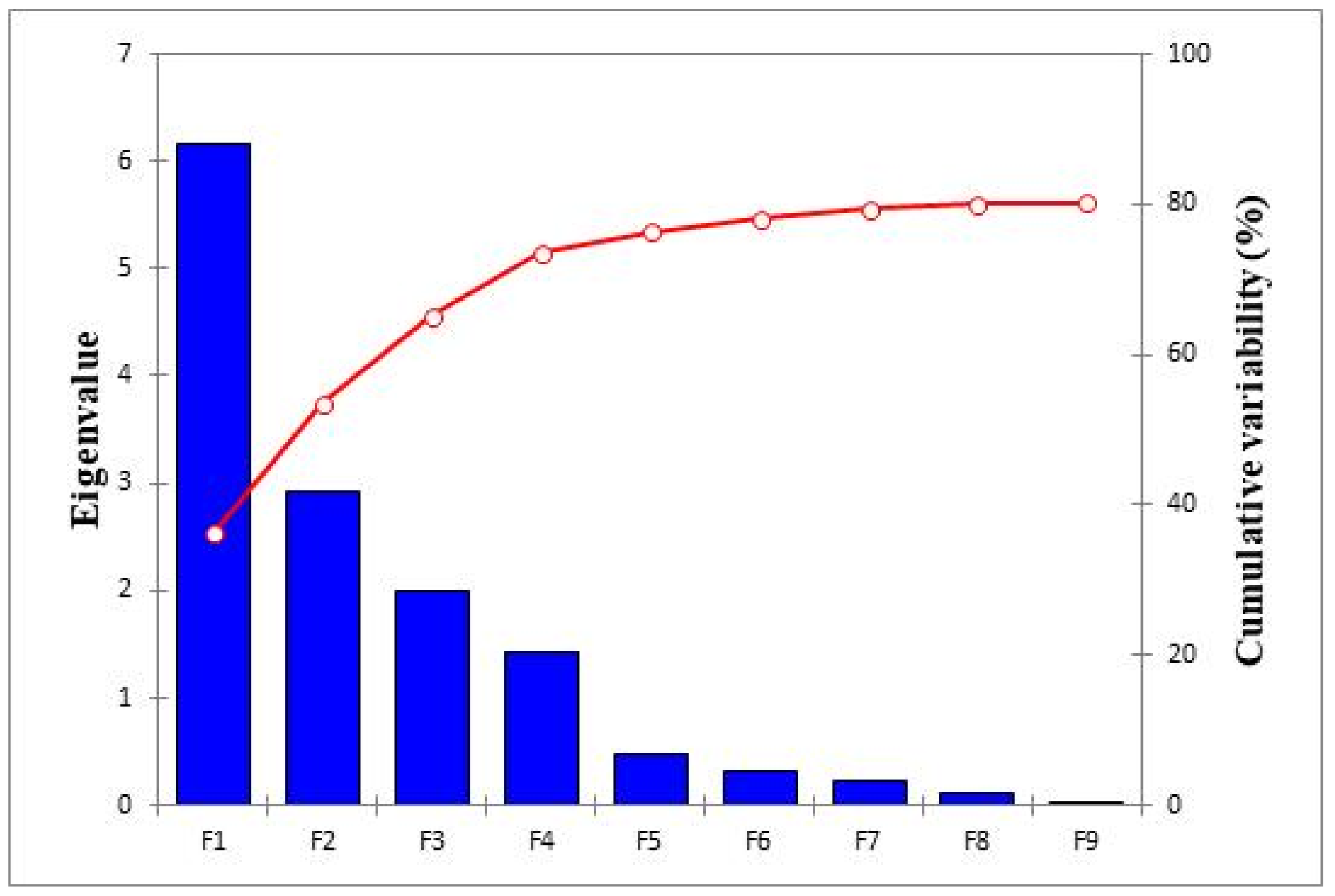
| Factor 1 | Factor 2 | Factor 3 | Factor 4 | |
| Variability (%) | 26.23 | 21.28 | 11.39 | 11.59 |
| Cumulative (%) | 26.23 | 47.51 | 58.90 | 70.50 |
| Variable | Factor 1 | Factor 2 | Factor 3 | Factor 4 | Communality |
| Z2 | −0.090 | 0.487 | 0.498 | −0.142 | 0.887 |
| Aav | −0.121 | −0.928 | 0.045 | 0.021 | 0.889 |
| I | −0.069 | −0.905 | −0.061 | 0.070 | 0.842 |
| NSA | 0.030 | 0.876 | −0.064 | −0.099 | 0.858 |
| FC | −0.104 | −0.008 | −0.417 | 0.054 | 0.447 |
| Index AgL | 0.084 | −0.064 | 0.836 | −0.008 | 0.941 |
| Index ArL | −0.017 | 0.328 | 0.801 | −0.026 | 0.800 |
| ArLs | −0.043 | 0.819 | 0.252 | 0.003 | 0.810 |
| GDAgL | 0.307 | −0.013 | 0.026 | 0.870 | 0.872 |
| SDArL | 0.327 | −0.233 | −0.036 | 0.885 | 1.000 |
| Index RP | 0.790 | −0.142 | 0.189 | 0.339 | 0.866 |
| DRP | 0.701 | 0.130 | −0.071 | 0.412 | 0.775 |
| Index V | 0.951 | 0.117 | −0.009 | 0.093 | 0.951 |
| RPav | −0.831 | −0.025 | 0.052 | −0.019 | 0.776 |
| ORP | −0.909 | −0.147 | 0.056 | −0.033 | 0.889 |
| Index H | 0.818 | −0.144 | 0.158 | 0.304 | 0.970 |
| Index Hs | −0.048 | −0.011 | 0.164 | 0.070 | 0.111 |
| Z2 | Aav | I | NSA | FC | Index AgL | Index ArL | ArLs | GDAgL | SDArL | Index RP | DRP | Index V | RPav | ORP | Index H | Index Hs | |
| Z2 | 1 | ||||||||||||||||
| Aav | −0.725 | 1 | |||||||||||||||
| I | −0.782 | 0.821 | 1 | ||||||||||||||
| NSA | 0.498 | −0.428 | −0.552 | 1 | |||||||||||||
| FC | −0.789 | 0.735 | 0.890 | −0.361 | 1 | ||||||||||||
| Index AgL | 0.409 | −0.383 | −0.474 | 0.179 | −0.561 | 1 | |||||||||||
| Index ArL | 0.254 | −0.250 | −0.240 | 0.276 | −0.222 | 0.685 | 1 | ||||||||||
| ArLs | 0.602 | −0.736 | −0.628 | 0.396 | −0.515 | 0.471 | 0.652 | 1 | |||||||||
| GDAgL | −0.134 | 0.170 | 0.054 | 0.121 | 0.157 | −0.249 | −0.213 | −0.257 | 1 | ||||||||
| SDArL | −0.145 | 0.186 | 0.065 | 0.112 | 0.167 | −0.253 | −0.222 | −0.274 | 0.998 | 1 | |||||||
| Index RP | −0.037 | −0.143 | −0.057 | 0.003 | −0.026 | −0.048 | −0.084 | −0.055 | −0.024 | −0.040 | 1 | ||||||
| DRP | 0.353 | −0.458 | −0.463 | 0.414 | −0.445 | 0.271 | 0.157 | 0.300 | −0.005 | −0.047 | 0.263 | 1 | |||||
| Index V | 0.095 | −0.368 | −0.355 | 0.244 | −0.267 | 0.343 | 0.289 | 0.338 | 0.047 | 0.021 | 0.348 | 0.536 | 1 | ||||
| RPav | −0.157 | 0.409 | 0.389 | −0.319 | 0.281 | −0.387 | −0.411 | −0.468 | −0.039 | −0.016 | −0.364 | −0.432 | −0.856 | 1 | |||
| ORP | −0.174 | 0.436 | 0.415 | −0.351 | 0.294 | −0.372 | −0.348 | −0.417 | −0.070 | −0.054 | −0.303 | −0.391 | −0.839 | 0.936 | 1 | ||
| Index H | −0.020 | −0.168 | −0.079 | −0.010 | −0.061 | −0.002 | −0.057 | −0.022 | −0.044 | −0.062 | 0.987 | 0.311 | 0.381 | −0.379 | −0.313 | 1 | |
| Index Hs | 0.124 | −0.255 | −0.311 | 0.367 | −0.181 | 0.173 | 0.238 | 0.218 | 0.184 | 0.158 | 0.455 | 0.435 | 0.634 | −0.741 | −0.696 | 0.393 | 1 |
| Factor 1 | Factor 2 | Factor 3 | Factor 4 | |
| Variability (%) | 25.23 | 22.24 | 13.26 | 12.74 |
| Cumulative (%) | 25.23 | 47.47 | 60.72 | 73.47 |
| Variable | Factor 1 | Factor 2 | Factor 3 | Factor 4 | Communality |
| Z2 | 0.888 | −0.007 | −0.084 | −0.047 | 0.798 |
| Aav | −0.818 | −0.236 | 0.134 | −0.106 | 0.755 |
| I | −0.935 | −0.208 | −0.008 | −0.037 | 0.918 |
| NSA | 0.508 | 0.271 | 0.157 | −0.048 | 0.359 |
| FC | −0.869 | −0.106 | 0.115 | −0.028 | 0.780 |
| Index AgL | 0.418 | 0.395 | −0.313 | −0.190 | 0.465 |
| Index ArL | 0.235 | 0.490 | −0.313 | −0.294 | 0.480 |
| ArLs | 0.614 | 0.396 | −0.293 | −0.193 | 0.657 |
| GDAgL | −0.063 | 0.074 | 0.969 | −0.040 | 0.950 |
| SDArL | −0.076 | 0.053 | 0.964 | −0.055 | 0.941 |
| Index RP | −0.011 | 0.226 | −0.028 | 0.943 | 0.942 |
| DRP | 0.432 | 0.362 | 0.021 | 0.245 | 0.378 |
| Index V | 0.172 | 0.816 | 0.021 | 0.230 | 0.748 |
| RPav | −0.189 | −0.946 | 0.001 | −0.178 | 0.962 |
| ORP | −0.221 | −0.881 | −0.050 | −0.142 | 0.847 |
| Index H | 0.015 | 0.236 | −0.059 | 0.915 | 0.897 |
| Index Hs | 0.159 | 0.680 | 0.182 | 0.304 | 0.613 |
Disclaimer/Publisher’s Note: The statements, opinions and data contained in all publications are solely those of the individual author(s) and contributor(s) and not of MDPI and/or the editor(s). MDPI and/or the editor(s) disclaim responsibility for any injury to people or property resulting from any ideas, methods, instructions or products referred to in the content. |
© 2023 by the authors. Licensee MDPI, Basel, Switzerland. This article is an open access article distributed under the terms and conditions of the Creative Commons Attribution (CC BY) license (https://creativecommons.org/licenses/by/4.0/).
Share and Cite
Srejić, T.; Manojlović, S.; Sibinović, M.; Bajat, B.; Novković, I.; Milošević, M.V.; Carević, I.; Todosijević, M.; Sedlak, M.G. Agricultural Land Use Changes as a Driving Force of Soil Erosion in the Velika Morava River Basin, Serbia. Agriculture 2023, 13, 778. https://doi.org/10.3390/agriculture13040778
Srejić T, Manojlović S, Sibinović M, Bajat B, Novković I, Milošević MV, Carević I, Todosijević M, Sedlak MG. Agricultural Land Use Changes as a Driving Force of Soil Erosion in the Velika Morava River Basin, Serbia. Agriculture. 2023; 13(4):778. https://doi.org/10.3390/agriculture13040778
Chicago/Turabian StyleSrejić, Tanja, Sanja Manojlović, Mikica Sibinović, Branislav Bajat, Ivan Novković, Marko V. Milošević, Ivana Carević, Mirjana Todosijević, and Marko G. Sedlak. 2023. "Agricultural Land Use Changes as a Driving Force of Soil Erosion in the Velika Morava River Basin, Serbia" Agriculture 13, no. 4: 778. https://doi.org/10.3390/agriculture13040778