
Real-Time Plant Health Detection Using Deep Convolutional Neural Networks
 , ,
, ,  and
and 
Abstract
:1. Introduction
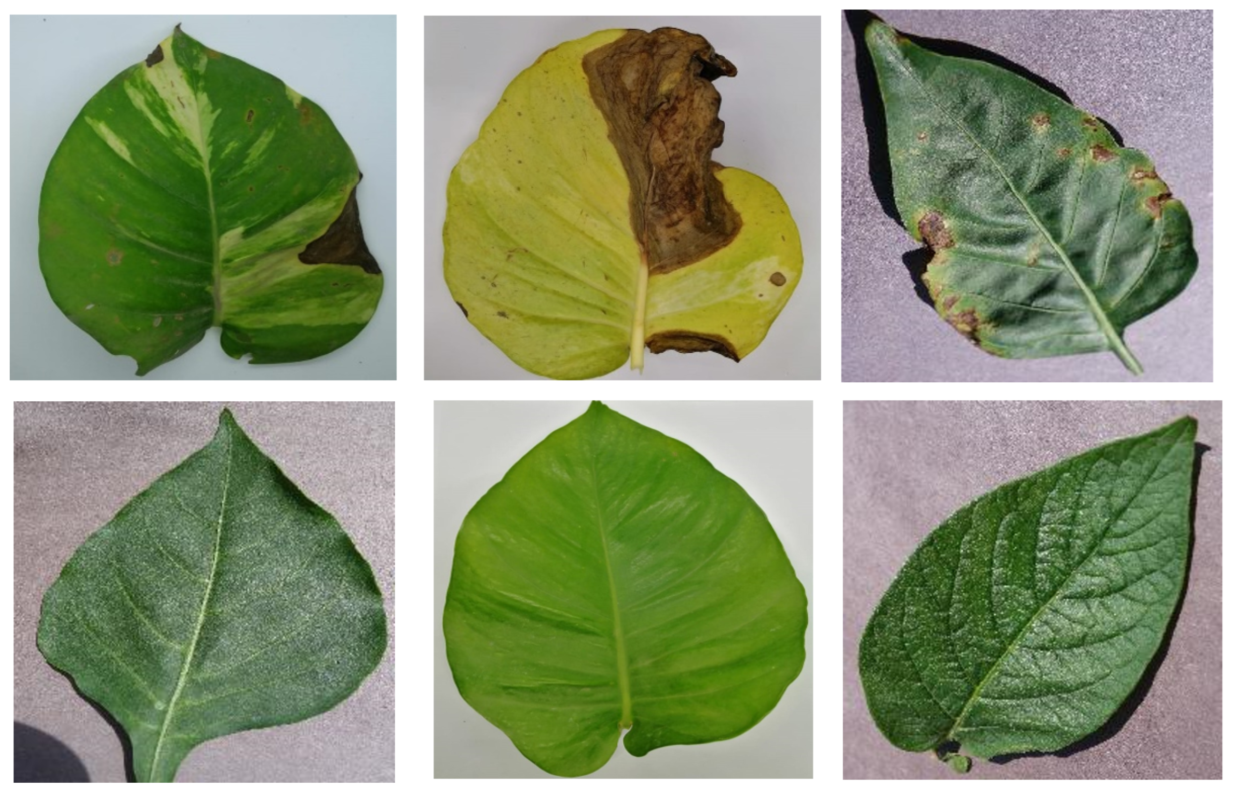
- A dataset with several scenarios and sizes was created. There were a variety of sophisticated backdrops, with varying lighting and perspectives, that featured images of damaged leaves. This offered the optimal information to make plant disease research easier.
- This study provided thorough, detailed literature on the methods currently used in plant disease identification. It also reviewed the literature on the datasets used in the research and provided a comparative analysis that identified various studies’ advantages and disadvantages.
- This study used different-deep-learning algorithms for the classification of plant anomalies.
- This study established the hyper-parameters for the applied deep algorithm for comparison with state-of-the-art plant disease classification algorithms (standard machine learning (ML) approaches)
- This study evaluated the applied deep-learning algorithm with standard efficiency parameters.
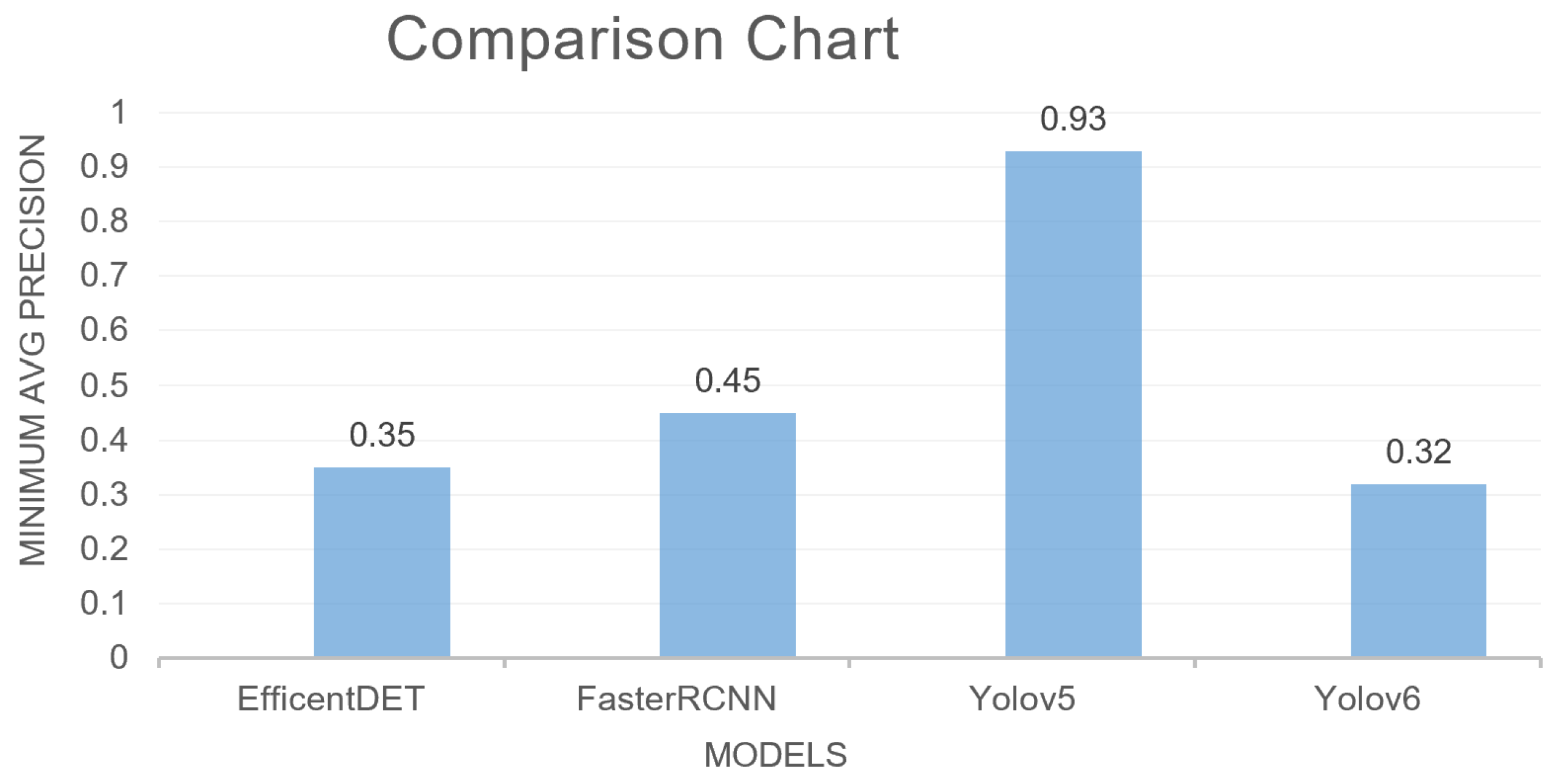
- This research evaluated 4 different target detection techniques, and the results of the trials demonstrated that the suggested approach achieved an mAP of 93.1% on both exclusive and public datasets at 120 frames per second (FPS). Precision planting, visual management, and intelligent decision-making were all features of the YOLOv5 algorithm for economic productivity.
2. Related Work
3. Comparative Analysis of Selected Study
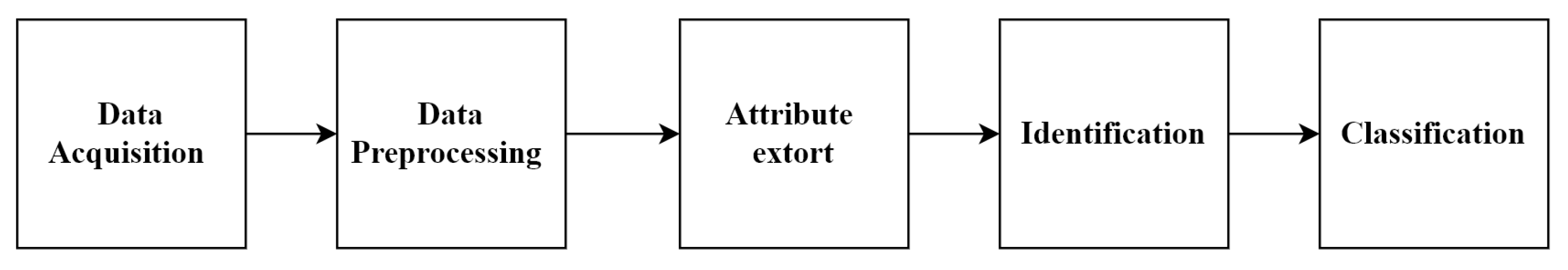
4. Materials and Methods
4.1. Experimental Material
4.2. Preprocessing on Exclusive Data Set
4.3. Preprocessing on Public Data Set
4.4. Plant Disease Detection and Classification Model Implementations
4.4.1. EfficentDet
4.4.2. FasterRCNN
4.4.3. The Principal of YOLOv5 Model
YOLO Versions
YOLOv5 Module
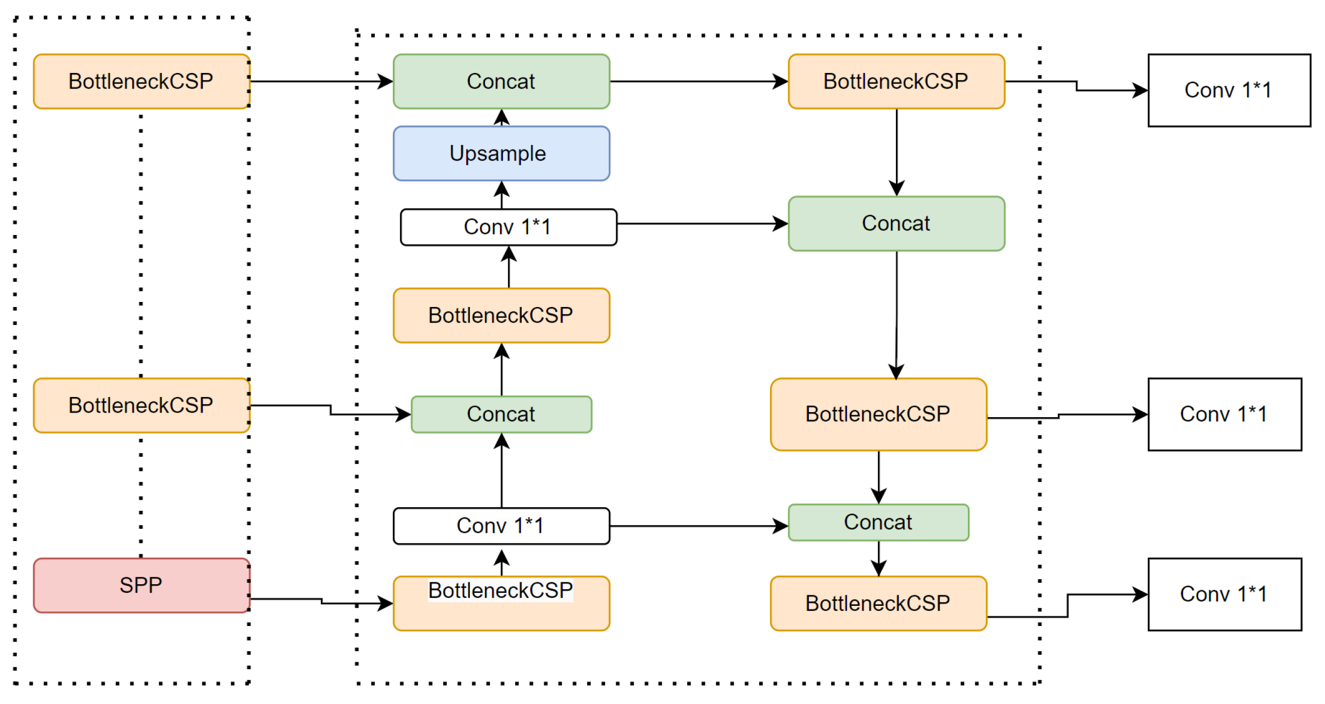
4.4.4. YOLOv5 Architecture
- 1.
- Backbone
- 2.
- Neck
- 3.
- Head
4.4.5. Activation Function
4.4.6. Optimization Function
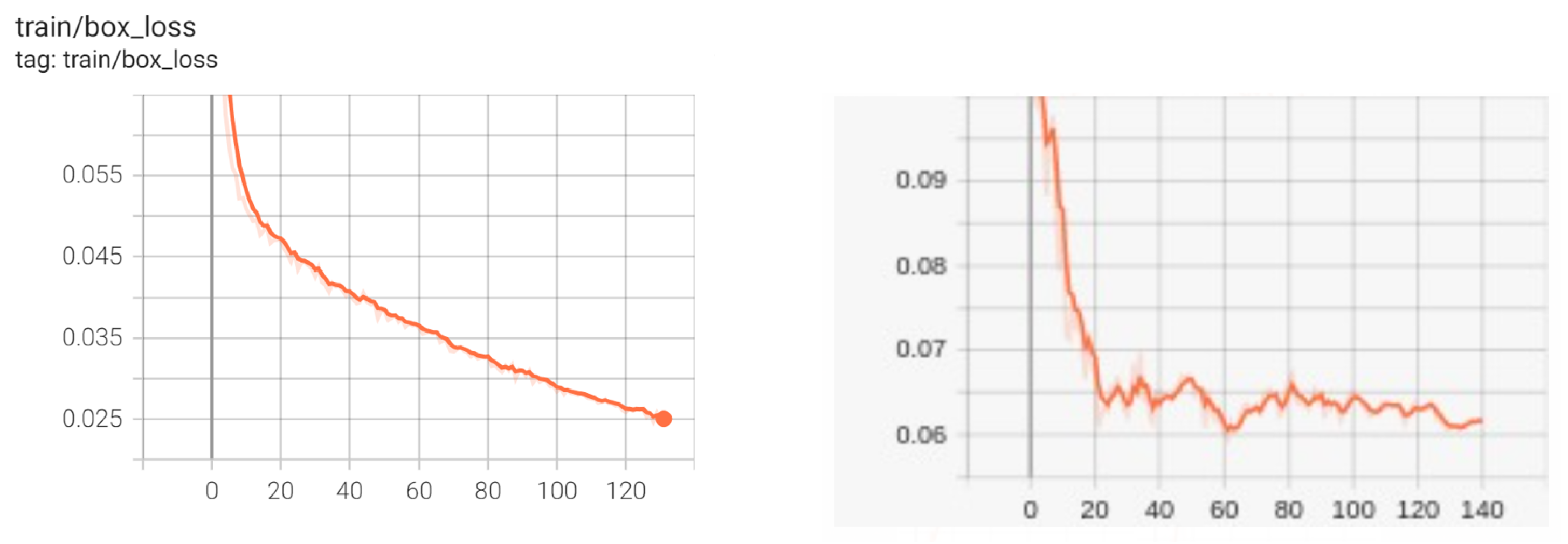
4.4.7. Cost Function or Loss Function
4.5. Training Exclusive and Public Datasets on YOLOv5
- 1.
- First step was the environment configuration for YOLO.
- 2.
- Obtaining the YOLOv5 repository and installing plugins were the initial steps. As a result, the programming framework was prepared for the execution of instructions for object identification training and inference.
- 3.
- We trained a model on the free training environment provided by Google Collab.
- 4.
- Google Collab was likely operating on a Tesla P100 GPU.
- 5.
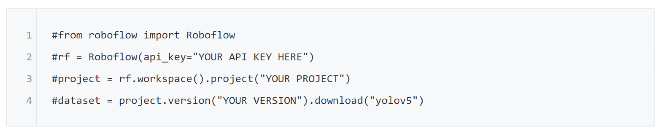
- Next, we downloaded the custom data from Roboflow in a YOLOv5 format.
- 6.
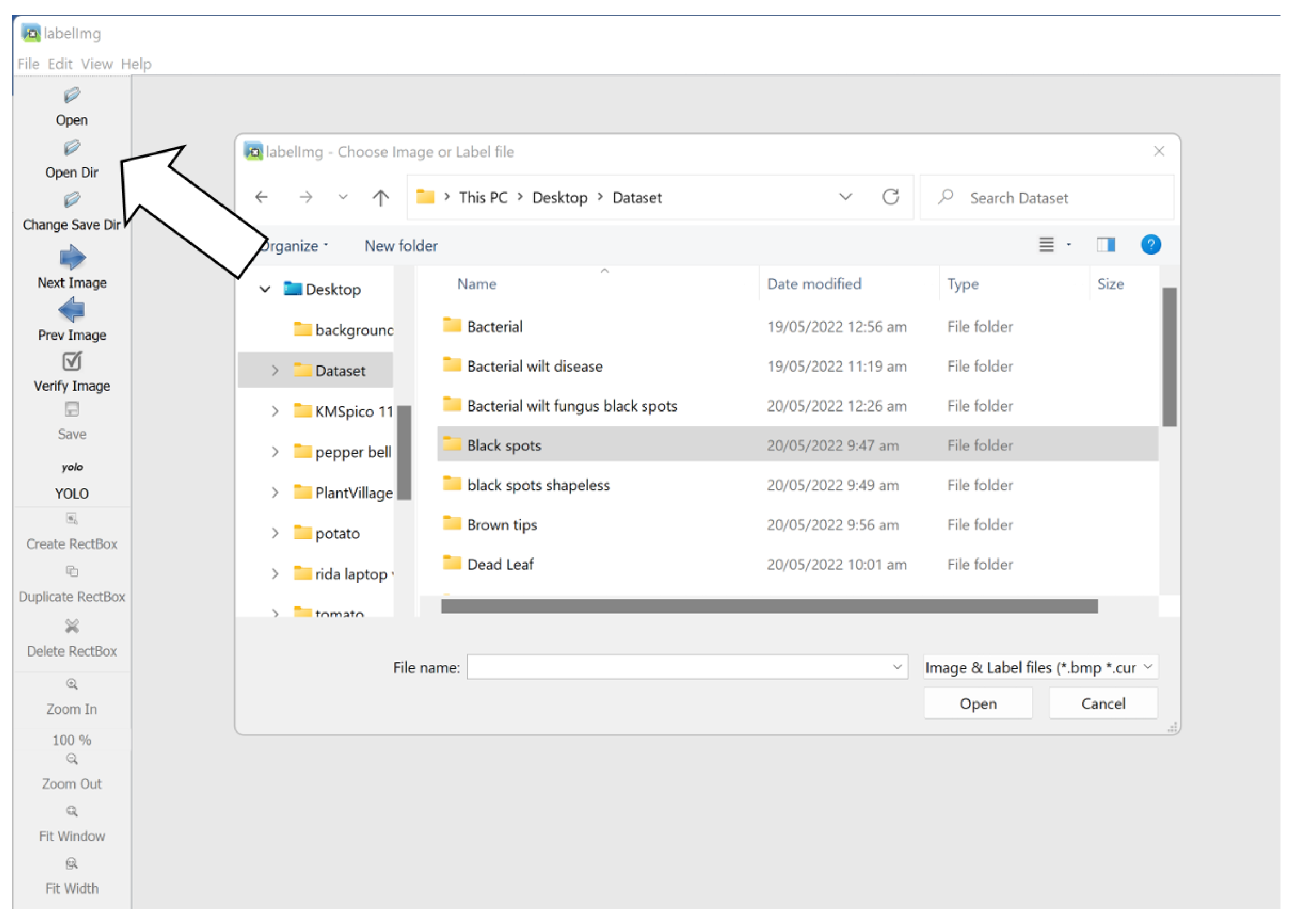
- After labeling the data, it was then exported to Roboflow. After uploading data into Roboflow, it was converted into one of these formats (VOC XML, coco json, TensorFlow object detection, etc.).
- 7.
- After uploading the data, we selected the preprocessing steps and augmentation.
- 8.
- Roboflow automatically divided the data into training, testing, and validation sets.
- 9.
- After annotating the images, we chose the YOLOv5 pyTorch format.
- 10.
- After the format steps, Roboflow provided a key or PIP package, as shown in Figure 10.
YOLOv5 Evaluation and Validation Metrics
4.6. YOLOv6
5. Results and Analysis
5.1. Dataset Validation Results
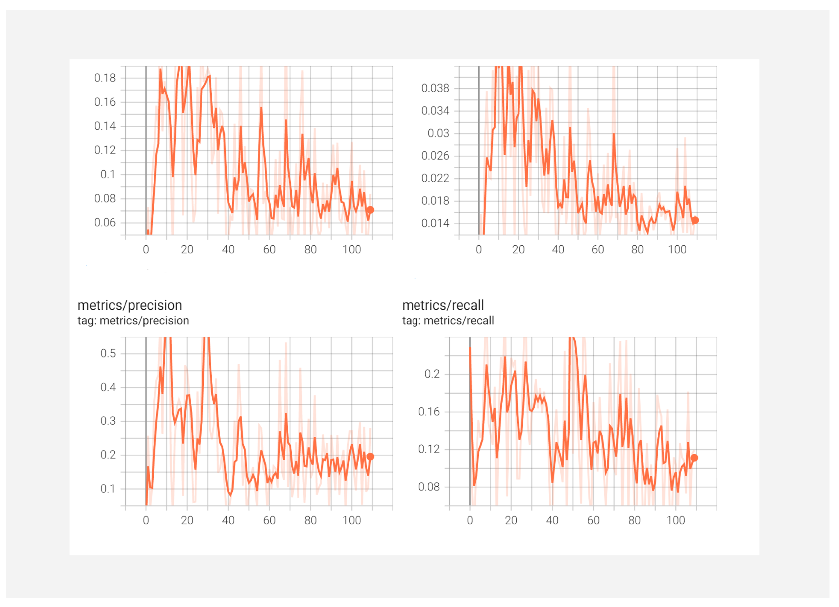
5.2. FasterRCNN
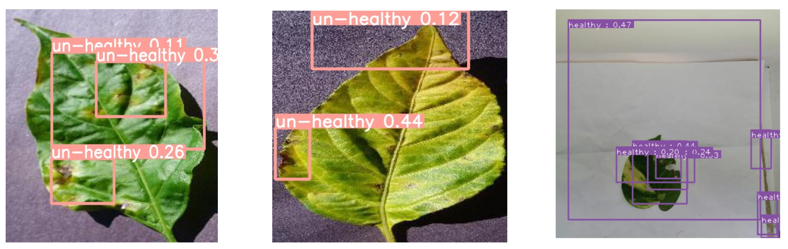
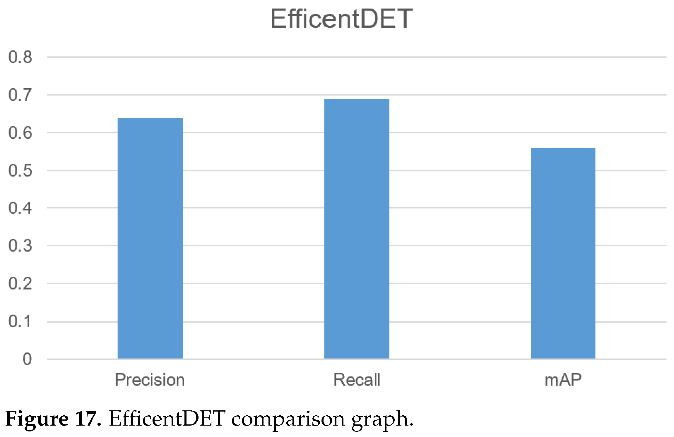
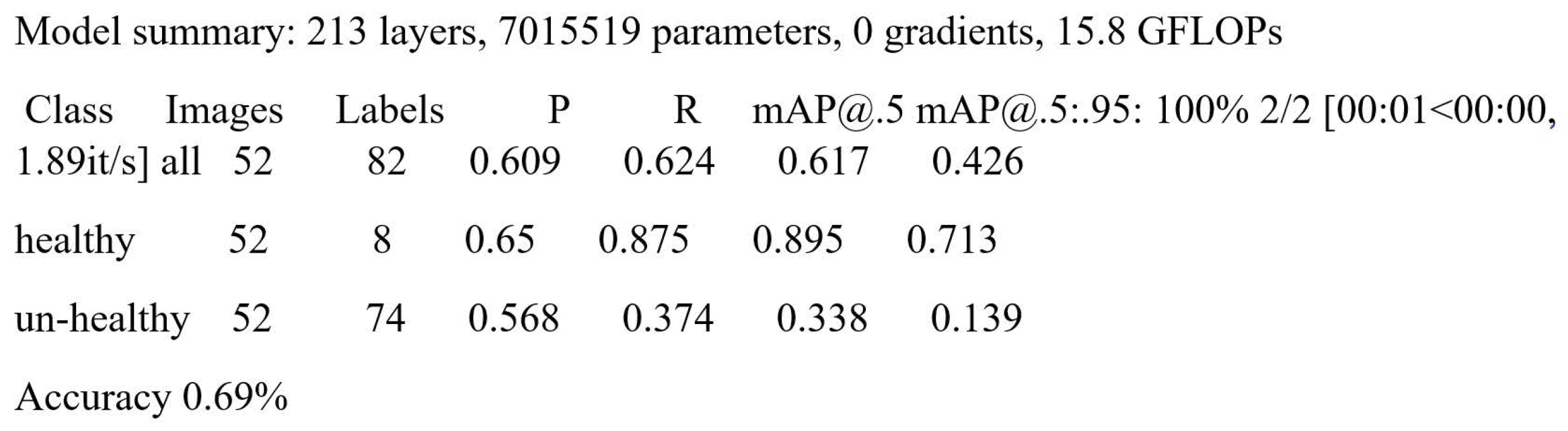
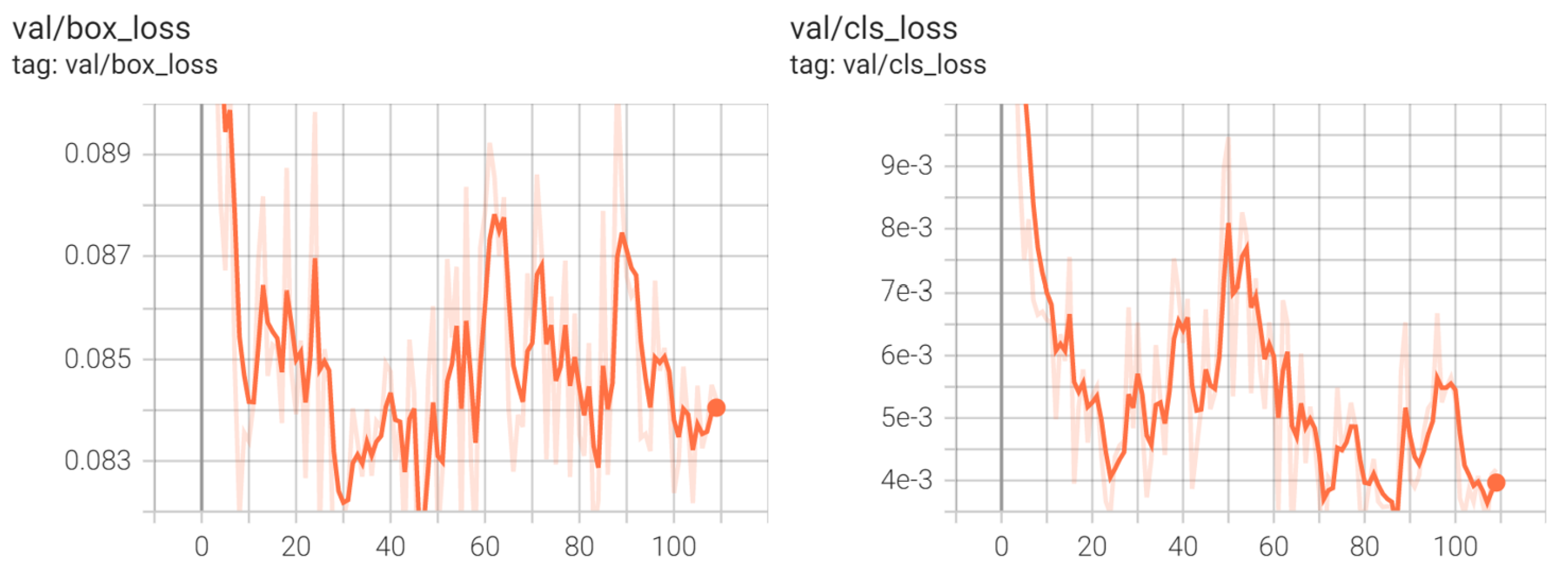
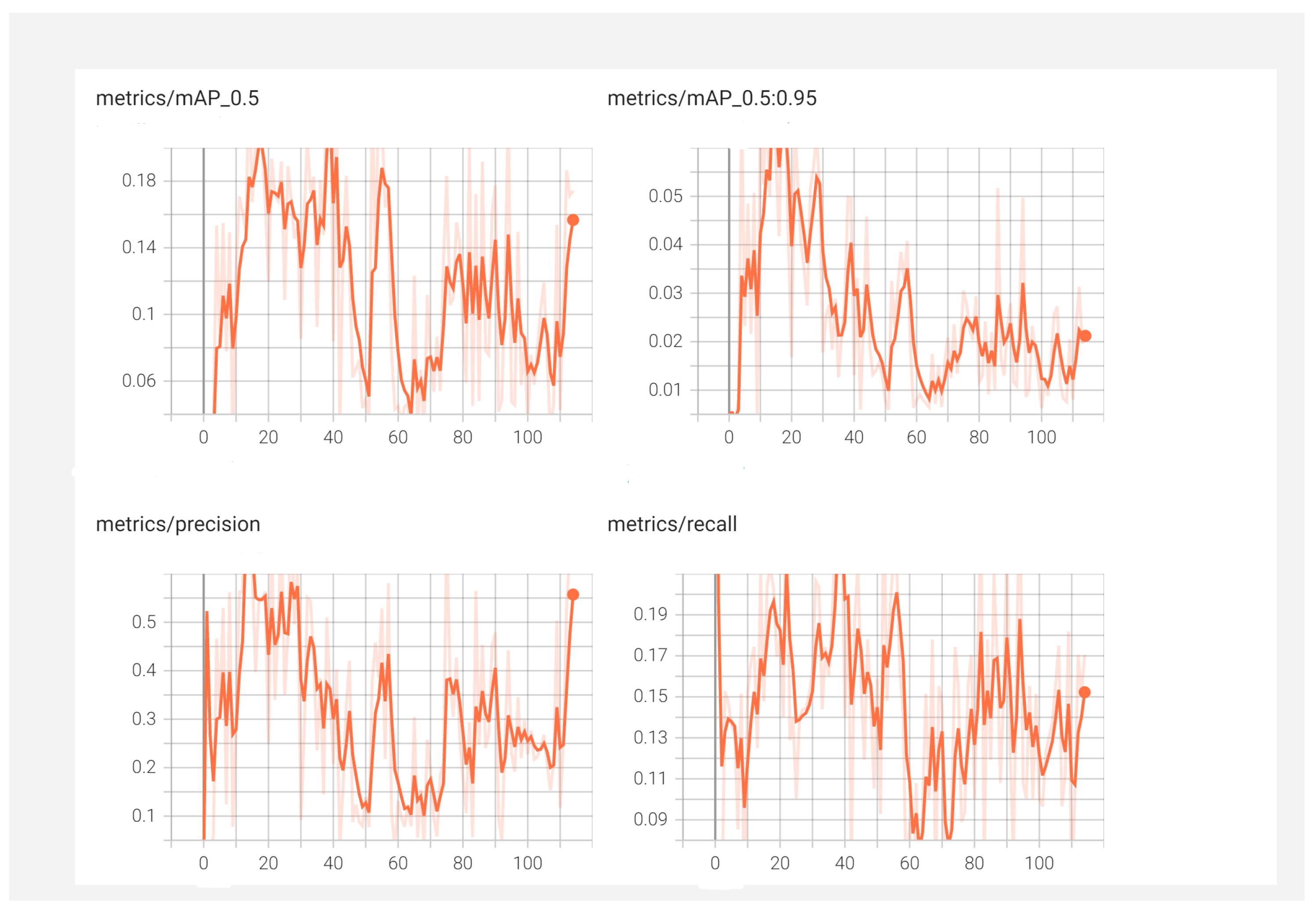
5.3. EfficentDET
5.4. YOLOv5 Experiments on Exclusive and Public Datasets
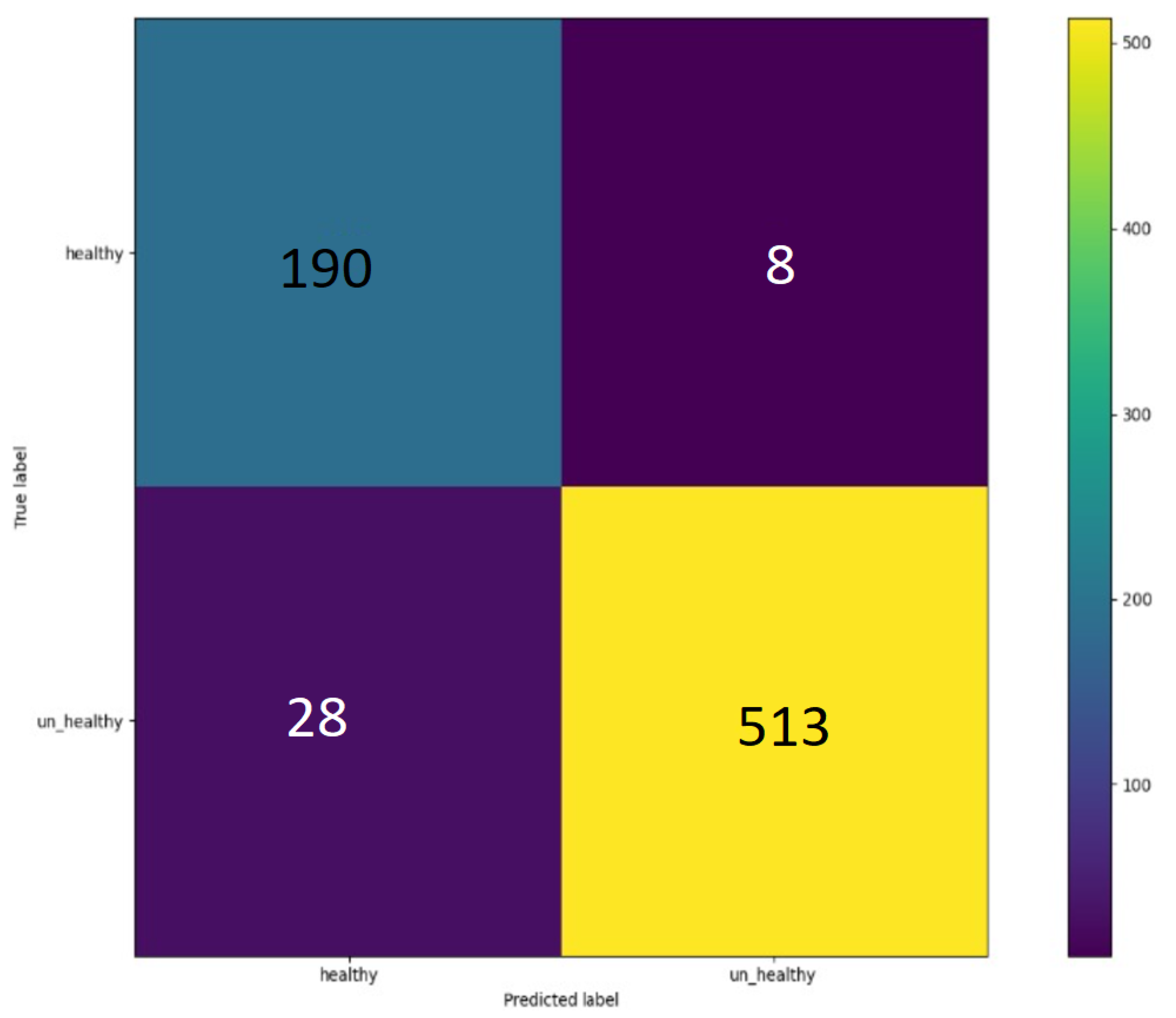
- (True Positive) = How many instances were accurately detected
- (False Positive) = Number of incorrectly identified cases between healthy and unhealthy leaves
- (False Negative) = Number of unidentified cases between healthy and unhealthy leave
- IOU = Intersection over union
- K = threshold
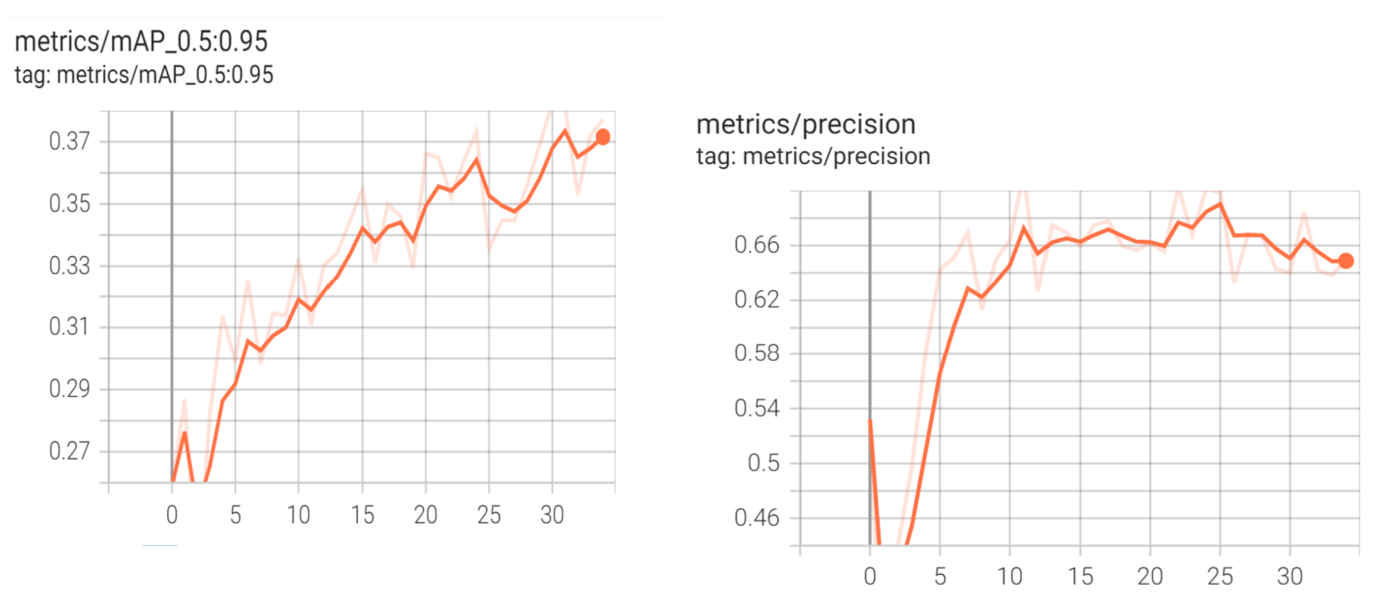
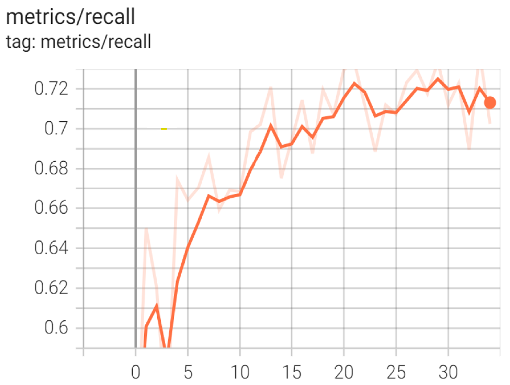
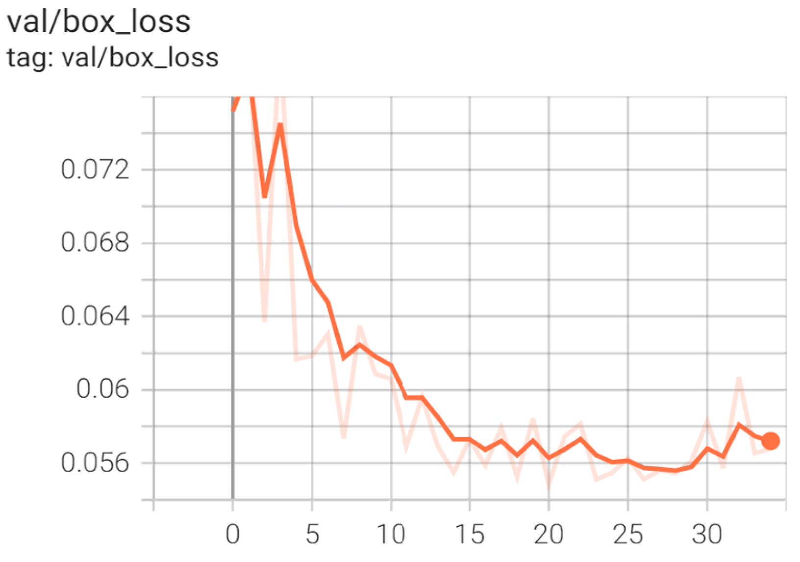
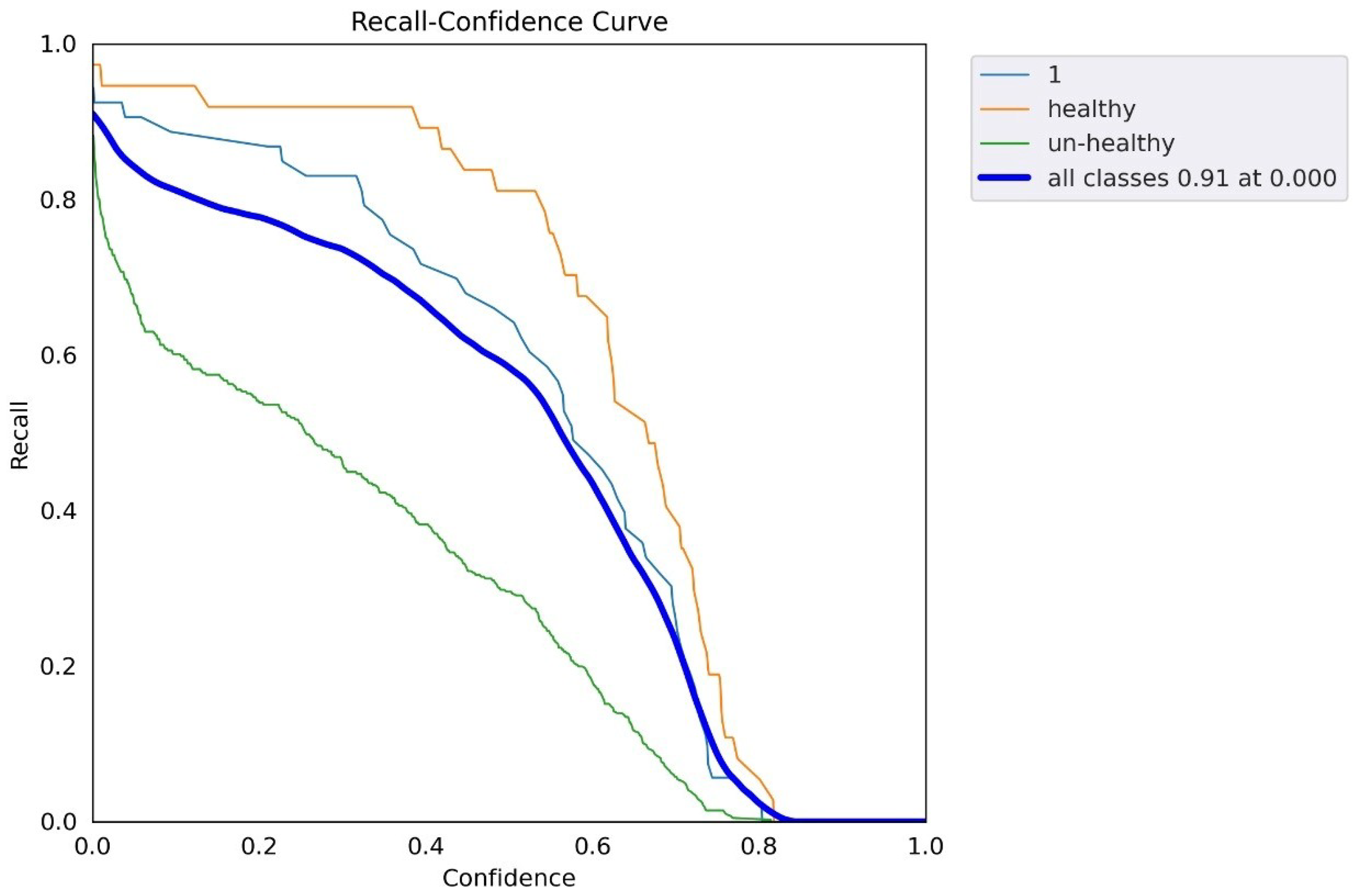
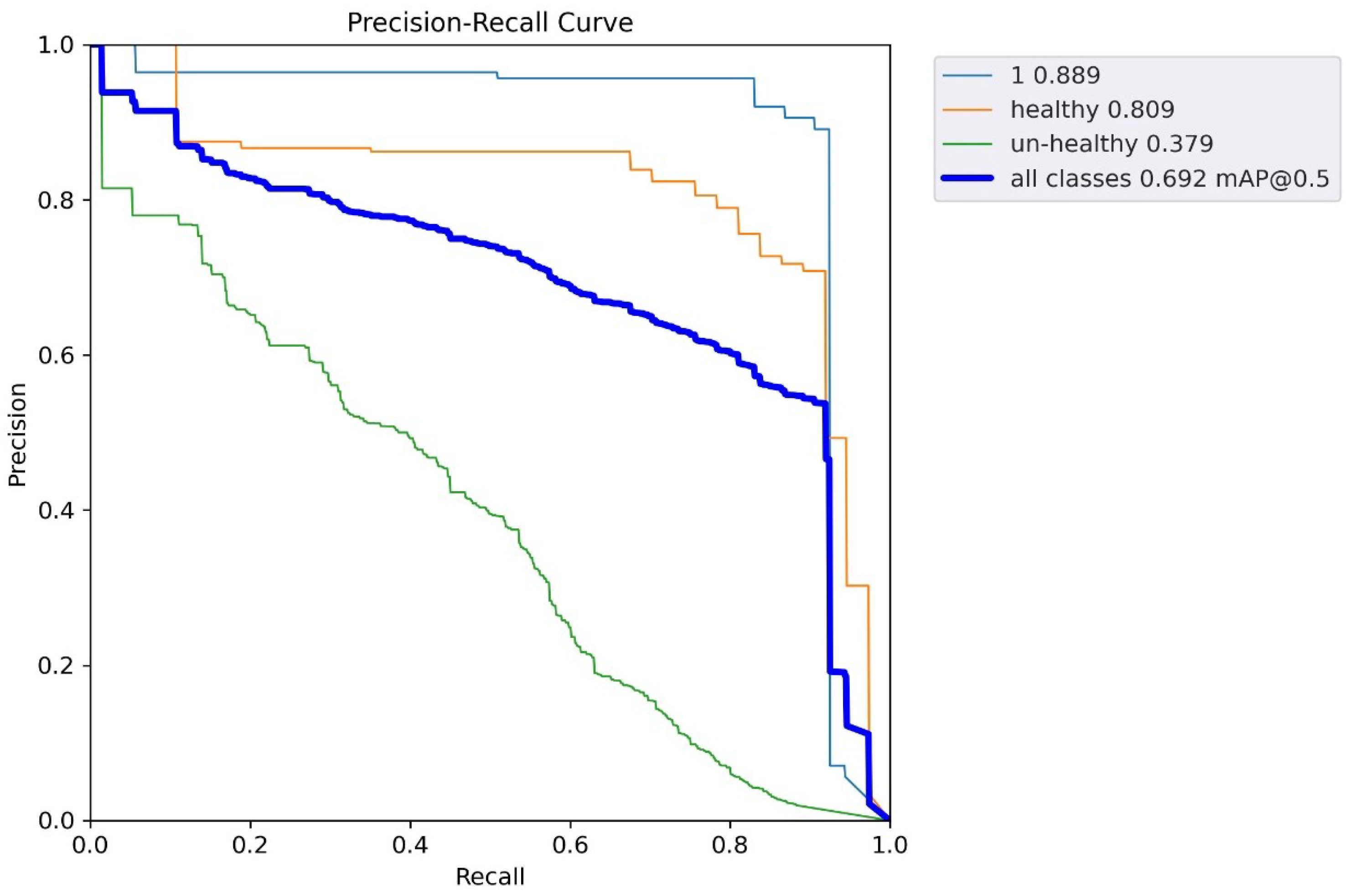
5.5. YOLOv5 Results
Confusion Matrix
5.6. Experiments on YOLOv6
5.7. Comparative Analysis
6. Conclusions
7. Limitations
Future Work
Author Contributions
Funding
Data Availability Statement
Conflicts of Interest
References
- Ferentinos, K.P. Deep learning models for plant disease detection and diagnosis. Comput. Electron. Agric. 2018, 145, 311–318. [Google Scholar] [CrossRef]
- Deng, L.; Deng, Q. The basic roles of indoor plants in human health and comfort. Environ. Sci. Pollut. Res. 2018, 25, 36087–36101. [Google Scholar] [CrossRef]
- Balasundram, S.K.; Golhani, K.; Shamshiri, R.R.; Vadamalai, G. Precision agriculture technologies for management of plant diseases. In Plant Disease Management Strategies for Sustainable Agriculture through Traditional and Modern Approaches; Springer: Berlin/Heidelberg, Germany, 2020; pp. 259–278. [Google Scholar]
- Trivedi, P.; Leach, J.E.; Tringe, S.G.; Sa, T.; Singh, B.K. Plant–microbiome interactions: From community assembly to plant health. Nat. Rev. Microbiol. 2020, 18, 607–621. [Google Scholar] [CrossRef] [PubMed]
- Wang, X.; Yang, W.; Wheaton, A.; Cooley, N.; Moran, B. Efficient registration of optical and IR images for automatic plant water stress assessment. Comput. Electron. Agric. 2010, 74, 230–237. [Google Scholar] [CrossRef]
- Khan, S.; Narvekar, M.; Hasan, M.; Charolia, A.; Khan, A. Image processing based application of thermal imaging for monitoring stress detection in tomato plants. In Proceedings of the 2019 International Conference on Smart Systems and Inventive Technology (ICSSIT), Tirunelveli, India, 27–29 November 2019; IEEE: New York, NY, USA, 2019; pp. 1111–1116. [Google Scholar]
- Hasan, R.I.; Yusuf, S.M.; Alzubaidi, L. Review of the state of the art of deep learning for plant diseases: A broad analysis and discussion. Plants 2020, 9, 1302. [Google Scholar] [CrossRef] [PubMed]
- Arivazhagan, S.; Shebiah, R.N.; Ananthi, S.; Varthini, S.V. Detection of unhealthy region of plant leaves and classification of plant leaf diseases using texture features. Agric. Eng. Int. CIGR J. 2013, 15, 211–217. [Google Scholar]
- Lin, K.; Gong, L.; Huang, Y.; Liu, C.; Pan, J. Deep learning-based segmentation and quantification of cucumber powdery mildew using convolutional neural network. Front. Plant Sci. 2019, 10, 155. [Google Scholar] [CrossRef] [Green Version]
- Blumenthal, J.; Megherbi, D.B.; Lussier, R. Supervised machine learning via Hidden Markov Models for accurate classification of plant stress levels & types based on imaged Chlorophyll fluorescence profiles & their rate of change in time. In Proceedings of the 2017 IEEE International Conference on Computational Intelligence and Virtual Environments for Measurement Systems and Applications (CIVEMSA), Annecy, France, 26–28 June 2017; IEEE: New York, NY, USA, 2017; pp. 211–216. [Google Scholar]
- Shrivastava, V.K.; Pradhan, M.K. Rice plant disease classification using color features: A machine learning paradigm. J. Plant Pathol. 2021, 103, 17–26. [Google Scholar] [CrossRef]
- Chen, M.; Tang, Y.; Zou, X.; Huang, K.; Huang, Z.; Zhou, H.; Wang, C.; Lian, G. Three-dimensional perception of orchard banana central stock enhanced by adaptive multi-vision technology. Comput. Electron. Agric. 2020, 174, 105508. [Google Scholar] [CrossRef]
- Li, Q.; Jia, W.; Sun, M.; Hou, S.; Zheng, Y. A novel green apple segmentation algorithm based on ensemble U-Net under complex orchard environment. Comput. Electron. Agric. 2021, 180, 105900. [Google Scholar] [CrossRef]
- Mishra, M.; Choudhury, P.; Pati, B. Modified ride-NN optimizer for the IoT based plant disease detection. J. Ambient Intell. Humaniz. Comput. 2021, 12, 691–703. [Google Scholar] [CrossRef]
- Abisha, A.; Bharathi, N. Review on Plant health and Stress with various AI techniques and Big data. In Proceedings of the 2021 International Conference on System, Computation, Automation and Networking (ICSCAN), Puducherry, India, 30–31 July 2021; IEEE: New York, NY, USA, 2021; pp. 1–6. [Google Scholar]
- Chandel, N.S.; Chakraborty, S.K.; Rajwade, Y.A.; Dubey, K.; Tiwari, M.K.; Jat, D. Identifying crop water stress using deep-learning models. Neural Comput. Appl. 2021, 33, 5353–5367. [Google Scholar] [CrossRef]
- Jiang, B.; Wang, P.; Zhuang, S.; Li, M.; Gong, Z. Drought stress detection in the middle growth stage of maize based on gabor filter and deep learning. In Proceedings of the 2019 Chinese Control Conference (CCC), Guangzhou, China, 27–30 July 2019; IEEE: New York, NY, USA, 2019; pp. 7751–7756. [Google Scholar]
- Ahmed, F.; Al-Mamun, H.A.; Bari, A.H.; Hossain, E.; Kwan, P. Classification of crops and weeds from digital images: A support vector machine approach. Crop Prot. 2012, 40, 98–104. [Google Scholar] [CrossRef]
- Abdulridha, J.; Ehsani, R.; Abd-Elrahman, A.; Ampatzidis, Y. A remote sensing technique for detecting laurel wilt disease in avocado in presence of other biotic and abiotic stresses. Comput. Electron. Agric. 2019, 156, 549–557. [Google Scholar] [CrossRef]
- Khan, R.U.; Khan, K.; Albattah, W.; Qamar, A.M. Image-based detection of plant diseases: From classical machine learning to deep learning journey. Wirel. Commun. Mob. Comput. 2021, 2021, 5541859. [Google Scholar] [CrossRef]
- Singh, D.; Jain, N.; Jain, P.; Kayal, P.; Kumawat, S.; Batra, N. PlantDoc: A dataset for visual plant disease detection. In Proceedings of the 7th ACM IKDD CoDS and 25th COMAD, Hyderabad, India, 5–7 January 2020; pp. 249–253. [Google Scholar]
- Mathew, M.P.; Mahesh, T.Y. Leaf-based disease detection in bell pepper plant using YOLOv5. Signal Image Video Process. 2022, 16, 841–847. [Google Scholar] [CrossRef]
- Khan, S.; Tufail, M.; Khan, M.T.; Khan, Z.A.; Anwar, S. Deep learning-based identification system of weeds and crops in strawberry and pea fields for a precision agriculture sprayer. Precis. Agric. 2021, 22, 1711–1727. [Google Scholar] [CrossRef]
- Wang, C.Y.; Bochkovskiy, A.; Liao, H.Y.M. Scaled-YOLOv4: Scaling cross stage partial network. In Proceedings of the IEEE/CVF Conference On Computer Vision and Pattern Recognition, Nashville, TN, USA, 20–25 June 2021; pp. 13029–13038. [Google Scholar]
- Redmon, J.; Farhadi, A. YOLOv3: An incremental improvement. arXiv 2018, arXiv:1804.02767. [Google Scholar]
- Paez, A.; Gebre, G.M.; Gonzalez, M.E.; Tschaplinski, T.J. Growth, soluble carbohydrates, and aloin concentration of Aloe vera plants exposed to three irradiance levels. Environ. Exp. Bot. 2000, 44, 133–139. [Google Scholar] [CrossRef] [PubMed]
- Jajja, A.I.; Abbas, A.; Khattak, H.A.; Niedbała, G.; Khalid, A.; Rauf, H.T.; Kujawa, S. Compact Convolutional Transformer (CCT)-Based Approach for Whitefly Attack Detection in Cotton Crops. Agriculture 2022, 12, 1529. [Google Scholar] [CrossRef]
- Niedbała, G.; Kurek, J.; Świderski, B.; Wojciechowski, T.; Antoniuk, I.; Bobran, K. Prediction of Blueberry (Vaccinium corymbosum L.) Yield Based on Artificial Intelligence Methods. Agriculture 2022, 12, 2089. [Google Scholar] [CrossRef]
- Jasim, M.A.; Al-Tuwaijari, J.M. Plant leaf diseases detection and classification using image processing and deep-learning techniques. In Proceedings of the 2020 International Conference on Computer Science and Software Engineering (CSASE), Duhok, Iraq, 16–18 April 2020; IEEE: New York, NY, USA, 2020; pp. 259–265. [Google Scholar]
- Swain, S.; Nayak, S.K.; Barik, S.S. A review on plant leaf diseases detection and classification based on machine learning models. Mukt Shabd 2020, 9, 5195–5205. [Google Scholar]
- Ranjan, M.; Weginwar, M.R.; Joshi, N.; Ingole, A. Detection and classification of leaf disease using artificial neural network. Int. J. Tech. Res. Appl. 2015, 3, 331–333. [Google Scholar]
- Bolliger, P.; Ostermaier, B. Koubachi: A mobile phone widget to enable affective communication with indoor plants. In Proceedings of the Mobile Interaction with the Real World (MIRW 2007), Singapore, 9 September 2007; p. 63. [Google Scholar]
- Gélard, W.; Herbulot, A.; Devy, M.; Casadebaig, P. 3D leaf tracking for plant growth monitoring. In Proceedings of the 2018 25th IEEE International Conference on Image Processing (ICIP), Athens, Greece, 7–10 October 2018; IEEE: New York, NY, USA, 2018; pp. 3663–3667. [Google Scholar]
- Mishra, P.; Feller, T.; Schmuck, M.; Nicol, A.; Nordon, A. Early detection of drought stress in Arabidopsis thaliana utilsing a portable hyperspectral imaging setup. In Proceedings of the 2019 10th Workshop on Hyperspectral Imaging and Signal Processing: Evolution in Remote Sensing (WHISPERS), Amsterdam, The Netherlands, 24–26 September 2019; IEEE: New York, NY, USA, 2019; pp. 1–5. [Google Scholar]
- Alexandridis, T.K.; Moshou, D.; Pantazi, X.E.; Tamouridou, A.A.; Kozhukh, D.; Castef, F.; Lagopodi, A.; Zartaloudis, Z.; Mourelatos, S.; de Santos, F.J.N.; et al. Olive trees stress detection using Sentinel-2 images. In Proceedings of the IGARSS 2019—2019 IEEE International Geoscience and Remote Sensing Symposium, Yokohama, Japan, 28 July–2 August 2019; IEEE: New York, NY, USA, 2019; pp. 7220–7223. [Google Scholar]
- Ciężkowski, W.; Kleniewska, M.; Chormański, J. Using Landsat 8 Images for The Wetland Water Stress Calculation: Upper Biebrza Case Study. In Proceedings of the IGARSS 2019—2019 IEEE International Geoscience and Remote Sensing Symposium, Yokohama, Japan, 28 July–2 August 2019; IEEE: New York, NY, USA, 2019; pp. 6867–6870. [Google Scholar]
- Bhugra, S.; Chaudhury, S.; Lall, B. Use of leaf colour for drought stress analysis in rice. In Proceedings of the 2015 Fifth National Conference on Computer Vision, Pattern Recognition, Image Processing and Graphics (NCVPRIPG), Patna, India, 16–19 December 2015; IEEE: New York, NY, USA, 2015; pp. 1–4. [Google Scholar]
- Ahmed, K.; Shahidi, T.R.; Alam, S.M.I.; Momen, S. Rice leaf disease detection using machine learning techniques. In Proceedings of the 2019 International Conference on Sustainable Technologies for Industry 4.0 (STI), Dhaka, Bangladesh, 24–25 December 2019; IEEE: New York, NY, USA, 2019; pp. 1–5. [Google Scholar]
- Zhang, K.; Wu, Q.; Liu, A.; Meng, X. Can deep learning identify tomato leaf disease? Adv. Multimed. 2018, 2018, 6710865. [Google Scholar] [CrossRef] [Green Version]
- Selvaraj, M.G.; Vergara, A.; Ruiz, H.; Safari, N.; Elayabalan, S.; Ocimati, W.; Blomme, G. AI-powered banana diseases and pest detection. Plant Methods 2019, 15, 92. [Google Scholar] [CrossRef] [Green Version]


| References | Year | Methodology | Dataset Size | Accuracy |
|---|---|---|---|---|
| [1] | 2018 | Deep learning | 87,848 images | 99.53% |
| [29] | 2021 | CNN | 20,636 | 98.029% |
| [30] | 2018 | Google net Reset | 54,306 | 99.35% |
| [31] | 2018 | ANN | Kaggle dataset | 80% |
| [32] | 2007 | IOT | Custom data | Good Acc. |
| [33] | 2018 | 3D leaf tracking | 12 plants | comparison |
| [34] | 2019 | HSI | 6 plants | comparison |
| [35] | 2019 | Remote sensing | Sentinel-2 | Fast, accurate |
| [36] | 2019 | Satellite images | Landsat 8 | Fast, accurate |
| [37] | 2016 | Machine learning | CR262, MTU | comparison |
| [38] | 2019 | Alex net | Apples, cherry | Layers convolution |
| [39] | 2018 | Alex Net | Tomato leaves | — |
| [40] | 2019 | SSD | Banana | RNN Improve |
| Ref | Model | Problem | Dataset |
|---|---|---|---|
| [15] | CNN | Plants emotions detection | Kaggle dataset |
| [16] | Google Net Alex Net Inception V3 | Disease detection using deep learning | Custom dataset |
| [19] | Image processing | Disease Detection in Avocado | Custom dataset |
| [21] | Mobile Net Faster RCNN | Early plant disease detection | Custom dataset |
| [22] | YOLOv5 | Bell-pepper disease detection | Bell-pepper custom dataset |
| [25] | YOLOv3 | Object detection in images | Kaggle dataset |
| [25] | YOLOv4 | Object detection in images | Kaggle dataset |
| Class No | Class | Class No | Class |
|---|---|---|---|
| 0 | Un-Healthy | 1 | Healthy |
| Training Sample | Testing Sample | Validation Sample | Total Sample |
|---|---|---|---|
| 2000 | 206 | 105 | 2311 |
| Model Name | Accuracy | No. of Images | Precision | Recall | Dataset |
|---|---|---|---|---|---|
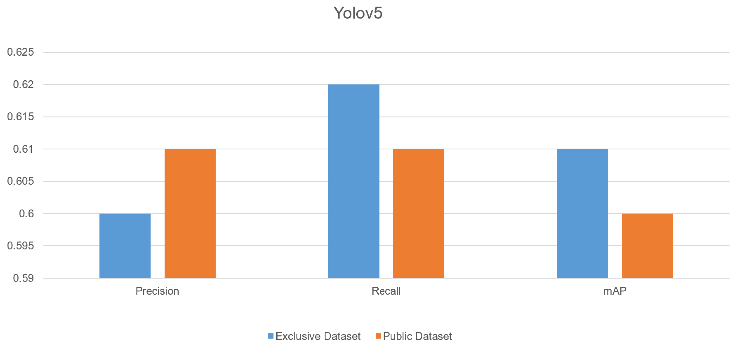
| YOLOv5 | 0.61 | 1k | 0.60 | 0.62 | Exclusive Dataset |
| Model Name | Accuracy | No. of Images | Precision | Recall | Dataset |
|---|---|---|---|---|---|
| YOLOv5 | 0.60 | 1k | 0.61 | 0.63 | Public Dataset |
| Model Name | Accuracy | No. of Images | Precision | Recall | Dataset |
|---|---|---|---|---|---|
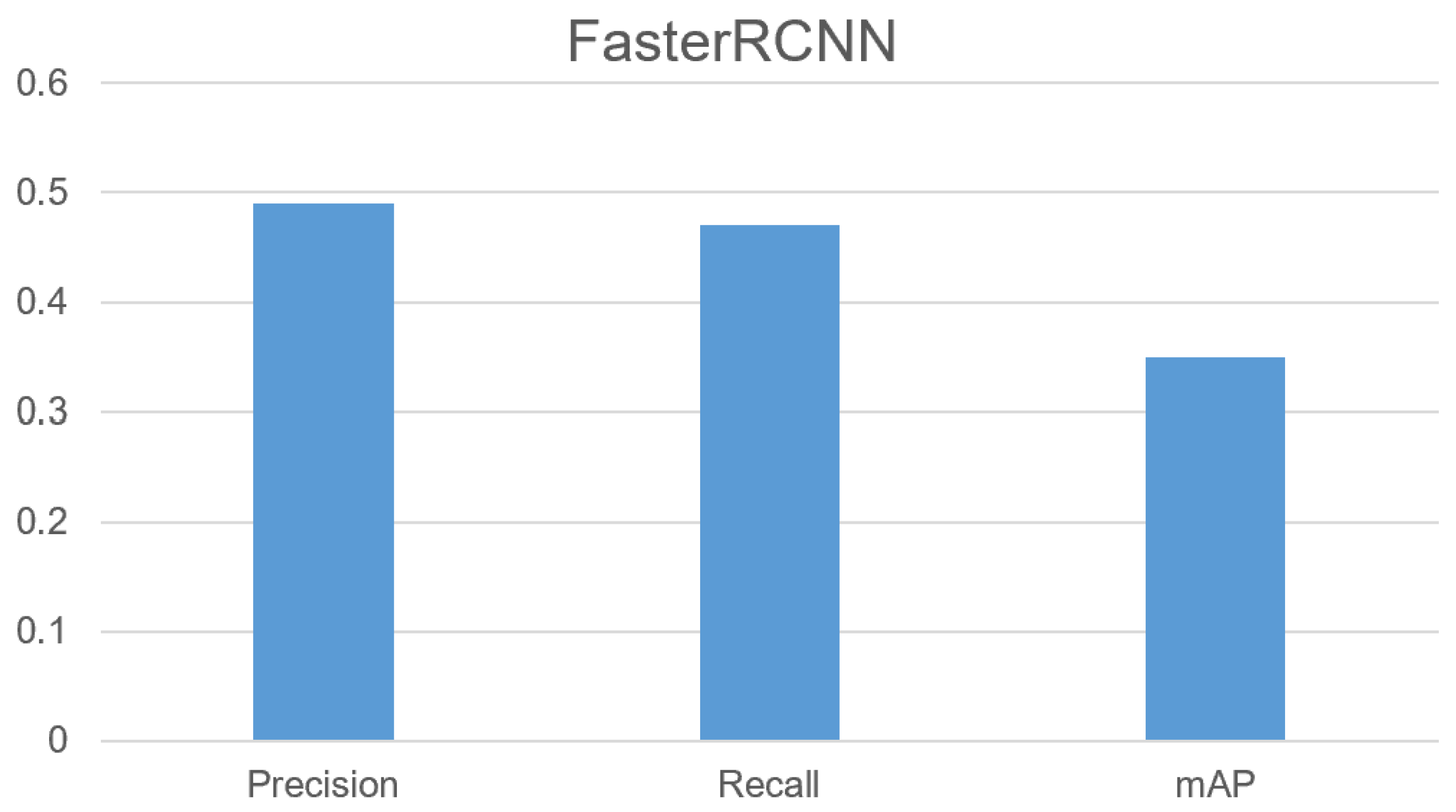
| FasterRCNN | 0.45 | 2k | 0.49 | 0.47 | Custom, public dataset |
| Model Name | Accuracy | No. of Images | Precision | Recall | Dataset |
|---|---|---|---|---|---|
| EfficentDET | 0.35 | 2k | 0.39 | 0.49 | Custom, public dataset |
| Model Name | Accuracy | No. of Images | Precision | Recall | Dataset |
|---|---|---|---|---|---|
| YOLOv5 | 0.93 | 2k | 0.75 | 0.95 | Custom, public dataset |
| Model Name | Accuracy | No. of Images | Precision | Recall | Dataset |
|---|---|---|---|---|---|
| YOLOv6 | 0.32 | 2k | 0.35 | 0.58 | Exclusive, Public dataset |
Disclaimer/Publisher’s Note: The statements, opinions and data contained in all publications are solely those of the individual author(s) and contributor(s) and not of MDPI and/or the editor(s). MDPI and/or the editor(s) disclaim responsibility for any injury to people or property resulting from any ideas, methods, instructions or products referred to in the content. |
© 2023 by the authors. Licensee MDPI, Basel, Switzerland. This article is an open access article distributed under the terms and conditions of the Creative Commons Attribution (CC BY) license (https://creativecommons.org/licenses/by/4.0/).
Share and Cite
Khalid, M.; Sarfraz, M.S.; Iqbal, U.; Aftab, M.U.; Niedbała, G.; Rauf, H.T. Real-Time Plant Health Detection Using Deep Convolutional Neural Networks. Agriculture 2023, 13, 510. https://doi.org/10.3390/agriculture13020510
Khalid M, Sarfraz MS, Iqbal U, Aftab MU, Niedbała G, Rauf HT. Real-Time Plant Health Detection Using Deep Convolutional Neural Networks. Agriculture. 2023; 13(2):510. https://doi.org/10.3390/agriculture13020510
Chicago/Turabian StyleKhalid, Mahnoor, Muhammad Shahzad Sarfraz, Uzair Iqbal, Muhammad Umar Aftab, Gniewko Niedbała, and Hafiz Tayyab Rauf. 2023. "Real-Time Plant Health Detection Using Deep Convolutional Neural Networks" Agriculture 13, no. 2: 510. https://doi.org/10.3390/agriculture13020510