

Intelligent Algorithm Optimization of Liquid Manure Spreading Control
Nanjing Institute of Agricultural Mechanization, Ministry of Agriculture and Rural Affairs, Nanjing 210014, China
*
Author to whom correspondence should be addressed.
Agriculture 2023, 13(2), 278; https://doi.org/10.3390/agriculture13020278
Submission received: 5 January 2023
/
Revised: 18 January 2023
/
Accepted: 19 January 2023
/
Published: 23 January 2023
(This article belongs to the Special Issue 'Eyes', 'Brain', 'Feet' and 'Hands' of Efficient Harvesting Machinery)
Abstract
:The growth of field crops needs appropriate soil nutrients. As a basic fertilizer, liquid manure provides biological nutrients for crop growth and increases the content of organic matter in crops. However, improper spraying not only reduces soil fertility but also destroys soil structure. Therefore, the precise control of the amount of liquid manure is of great significance for agricultural production and weight loss. In this study, we first built the model of spraying control, then optimized the BP neural network algorithm through a genetic algorithm. The stability and efficiency of the optimized controller were compared with PID, fuzzy PID and BPNN-PID control. The simulation results show that the optimized algorithm has the shortest response time and lowest relative error. Finally, platform experiments were designed to verify the four control algorithms at four different vehicle speeds. The results show that, compared with other control algorithms, the control algorithm described here has good stability, short response time, small overshoot, and can achieve an accurate fertilizer application effect, providing an optimization scheme for research on the precise application of liquid manure.
1. Introduction
The spraying of liquid manure is an important direction in precision agriculture research. This technology can address the issues of high labor intensity, low efficiency of throwing liquid organic manure, and uneven artificial fertilization [1,2,3]. Liquid manure contains a large amount of soluble nutrients and a variety of bioactive substances, such as amino acids and trace elements. The reasonable application of liquid manure can promote plant growth, increase yield, reduce fertilizer cost, raise soil organic matter content, and add soil chemical and physical latent capacity. Studies have shown that precision spraying technology can increase crop yield by 8–19% on average, reduce fertilizer application by approximately 30%, and improve soil quality [4,5,6]. At present, although the amount of liquid manure used is increasing annually worldwide, crop yields have not increased correspondingly. An analysis of liquid manure application indicates that the main reason for this is the large difference in the amount of liquid manure application per mu of land. Especially at the edge of the plot, the excessive application of liquid manure on some plots and the insufficient application of liquid manure on others due to manual control of fertilizer application or changes in vehicle speed directly affects the normal growth of crops in subsequent periods. In addition, excessive fertilization damages the soil structure and affects the growth environment and survival rate of crops. Hence, to increase the utilization coefficient of liquid manure and ensure the normal use of land resources, a more accurate and reasonable liquid manure spreading control technology should be adopted.
The main component of liquid manure is biogas slurry, which can be used to spread the base fertilizer in the field. Generally, the amount of basic fertilizer per hectare is 55 L. When biogas slurry is used as a basic fertilizer in the field, its dosage should be strictly controlled to prevent ammonia poisoning. Therefore, the precise application of liquid manure is fundamental and represents an important field of research within precision agriculture for the rapid and accurate adjustment of the amount of liquid manure fertilizer applied, as well as to maintain the set requirements. Research on precision fertilization mainly involves the optimization of algorithms and the establishment of a fertilization system model. At present, research on the control modeling of the fertilization process mainly includes nonlinear and linear artificial intelligence models. Within nonlinear control optimization, feedback linearization transformation control, adaptive regulation, and other methods are commonly used. Since over the traditional PID (proportion, integral, derivative) control method it is difficult to deal with complex nonlinear and hysteretic spraying control in the fertilizer transportation process, there is a need to develop a more intelligent optimization algorithm in order to precisely adjust and control the spraying process [7].
In the process of liquid manure spraying, most spraying controllers internally need an experience PID control strategy. However, in the actual spraying course, the driving speed and intelligent algorithm have a significant impact on the control system, leading to problems, including time variation and the hysteresis of the controlled object of the system, that cannot be solved. In this context, the traditional PID control algorithm is usually ineffective for variable spraying. A previous study [8] used the fuzzy neural network PID control of particle swarm optimization to adjust the fertilization system and found that the control algorithm had a small overshoot, excellent constancy, and a short rise time, which can bring about the aim of a good fertilization system. In another study [9], the authors proposed a fuzzy PID control method according to a genetic algorithm to address the problem of a long response time in the control process of an electric proportional valve. Their experimental verification identified the control method as superior to the traditional PID operating system together with the fuzzy PID control system. Another study [10] used traditional PID control to adjust the deviation and deviation rate of the PH value in fertilizer, and found that the cognoscenti PID control exhibited fine control behavior. Chang, C. et al. [11] aimed at the problem of pressure fluctuation caused by high-frequency opening and closing of valves during liquid fertilizer point application; they designed a high-frequency intermittent fertilizer supply system to optimize the system, and the parameters of the PID algorithm were adjusted using the critical proportion method. The system had certain stability. Li, T. et al. [12] put forward a way to precisely fertilize maize in view of the wavelet BP neural network algorithm to compute the non-linear matter of fertilization, which improved the accuracy of the optimal fertilization amount. In another study [13], the nonlinear model of the elastic BP neural network along with mixture gray wolf optimization was used for predictive control. The corresponding simulation dispatch demonstrated that the controller was capable of effectively diminishing the jam due to nonlinearity and exhibited a good performance. Xiuyun et al. [14] designed a variable-rate deep application system for liquid fertilizer based on ZigBee. ZigBee was used for networking and realizing short-distance wireless communication between upper and lower computers and achieved accurate fertilization by controlling the frequency of the variable-frequency pump. The control system was optimized using the incremental integral derivative algorithm, and the control effect was good. A previous study [15] proposed a simplified and linearized deep construction model based on theoretical considerations using frequency domain identification technology estimation. According to the dynamic changes of the system in the process of fertilization, the worst case of stability of the depth control system was found, and the parameters of the fertilization model were determined to achieve shallow and deep fertilization. Guangkun [16] designed a variable-rate fertilizer injection operating system for fluidity fertilizer that optimized the operating system by using a PID algorithm. With the wheeled-point fertilizer injector as the carrier, the authors achieved a good variable-rate fertilizer application effect. However, owing to the simple control algorithm, the control of the flow and pressure continued to have a large optimization space. Accordingly, in studies on the variable-rate spraying process control system of liquid manure, there are many control methods for valves and variable-frequency pumps, with most research methods optimizing the control of valves with PWM or using a PID algorithm. The fuzzy control and neural network control algorithms were studied based on PID control. In a traction-type liquid manure fertilizer applicator [10] with slow current velocity monitoring retroaction, the calculation of liquid fertilizer concentration, together with the reaction time of the solenoid valve to modify the opening of valve in line with the need, were discovered as significant elements to consider in the alternating-quantity spread manure control system [12,17,18].
With this kind of situation of automatically spread manure, the aim of this study is improve the accuracy of the amount of liquid manure in the process of spraying, as follows: (i) optimize the parameters of the spraying process; (ii) apply the BPNN–PID algorithm for optimizing dominant weight parameters; (iii) simulate and check the conventional PID dominants and BPNN–PID dominants, as well as BPNN–PID dominants optimized using a genetic algorithm on the MATLAB/Simulink plate; (iv) evidence the practicability as well as stability of the recommended algorithm. The outcome identified that the optimized dominate algorithm had fewer errors and shorter system response time than before.
The remainder of this paper is organized as follows. In the first part of this study, the control process of liquid manure spraying is analyzed and a transfer function model is established. The second part constructs the classical PID pilot together with the BPNN–PID pilot and optimizes the BPNN–PID using the genetic algorithm. First, the control signal is received and collected. After that, the BPNN system is built, as well as a genetic algorithm is used to multilayer the neural network. The third part contrasts the pilot impression of three pilot methods by way of software simulation along with test checking, as well as, lastly, achieving the experimental fruit of the liquid manure spraying control system based on the present investigation.
2. Materials and Methods
2.1. Working Principle of Liquid Manure Spreader
The liquid manure spreader used in this study was towed using a tractor, and the liquid manure was spread to the field ground through 12 spray pipes. The operating breadth of the fluidity manure spout pipe was 6 m and the driving velocity of the tractor used for towing varied from 1 to 2.5 m/s. An important part of the system for controlling the change in liquid manure flow was the electric proportional valve, which was installed at the front end of the fertilizer distributor. The distributor used in this study was a mass-production product with a uniform distribution. We did not need to consider its distribution uniformity and blockage but instead only needed to consider the open–shut sizes of the electric proportional gate controlled via computer to achieve accurate control of the liquid manure distribution. Based on the requirements for the accurate application of liquid manure, the principle of system flow control was based on the demand for liquid manure in the field. Turning on the solenoid valve was transformed by vehicle speed. The application amount was monitored using a fluid meter. Then, the data were coupled back to the regulator. The control formed a closed–cycle coupled-back uniform machine by analyzing and comparing the actual time runoff, the magnitude of fertilizer called for by the current plot, and the current vehicle speed, achieving an accurate control of the current plot spraying amount. The response accuracy and stability of the closed–cycle coupled-back uniformity machinery were the main influences of the exact fluidity manure spray control system in this study.
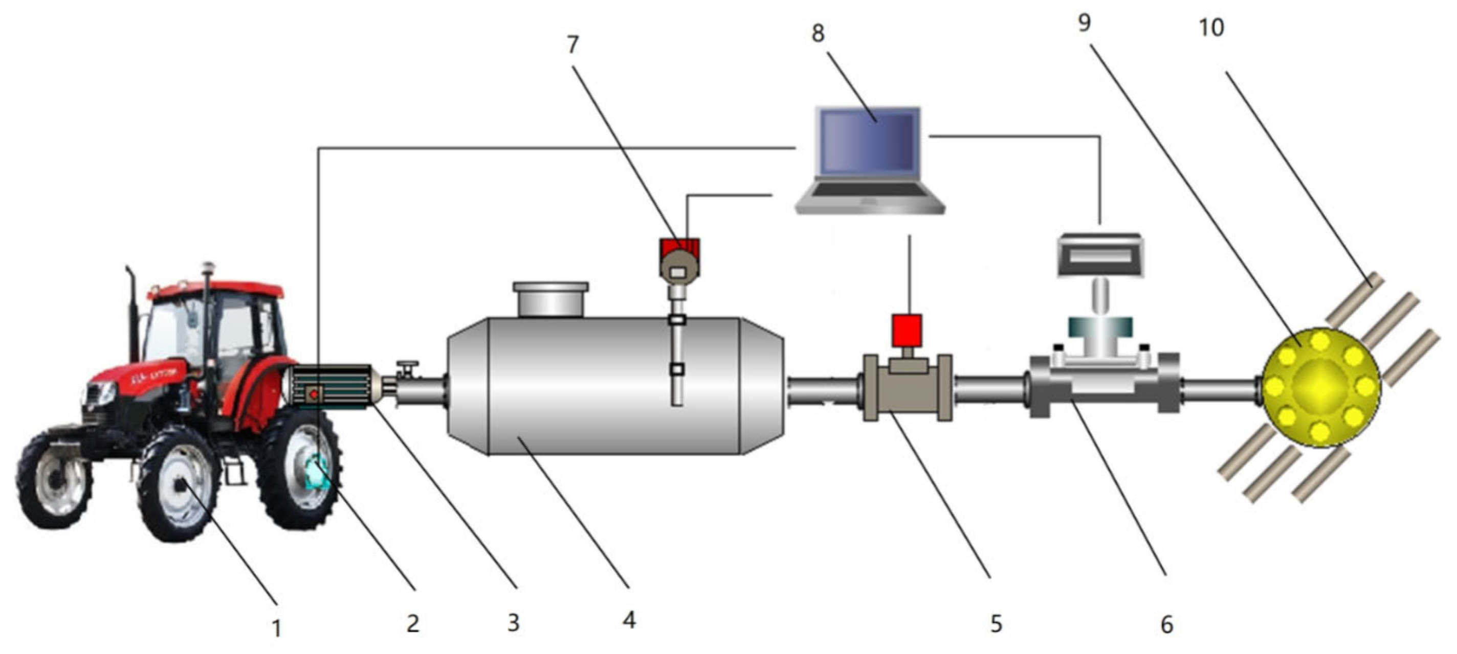
2.2. Equipment System Components
The formation of the manure spreading command equipment is exhibited in Figure 1. During fertilization, the chief command pattern, with the host computer as the main control unit, was used to control the open–shut the solenoid valve (Proportional solenoid valve, Shanghai Kaiweixi Co., Shanghai, China). An angular speed sensor (Analog output, Beijing Tianyuhengchuang Co., Beijing, China) was used to collect the wheel speed and convert it into the vehicle driving speed. The instantaneous flow rate of liquid manure was collected through the flowmeter as input data. The controller output the current signal to the solenoid valve after algorithm conversion. The solenoid valve was used to control valve opening, and the output of the system was the liquid manure flow. Then, the real–time data collected with the fluid meter were coupled back to the regulator, through which the closed–loop negative feedback control was realized.
2.3. Control System Model Construction
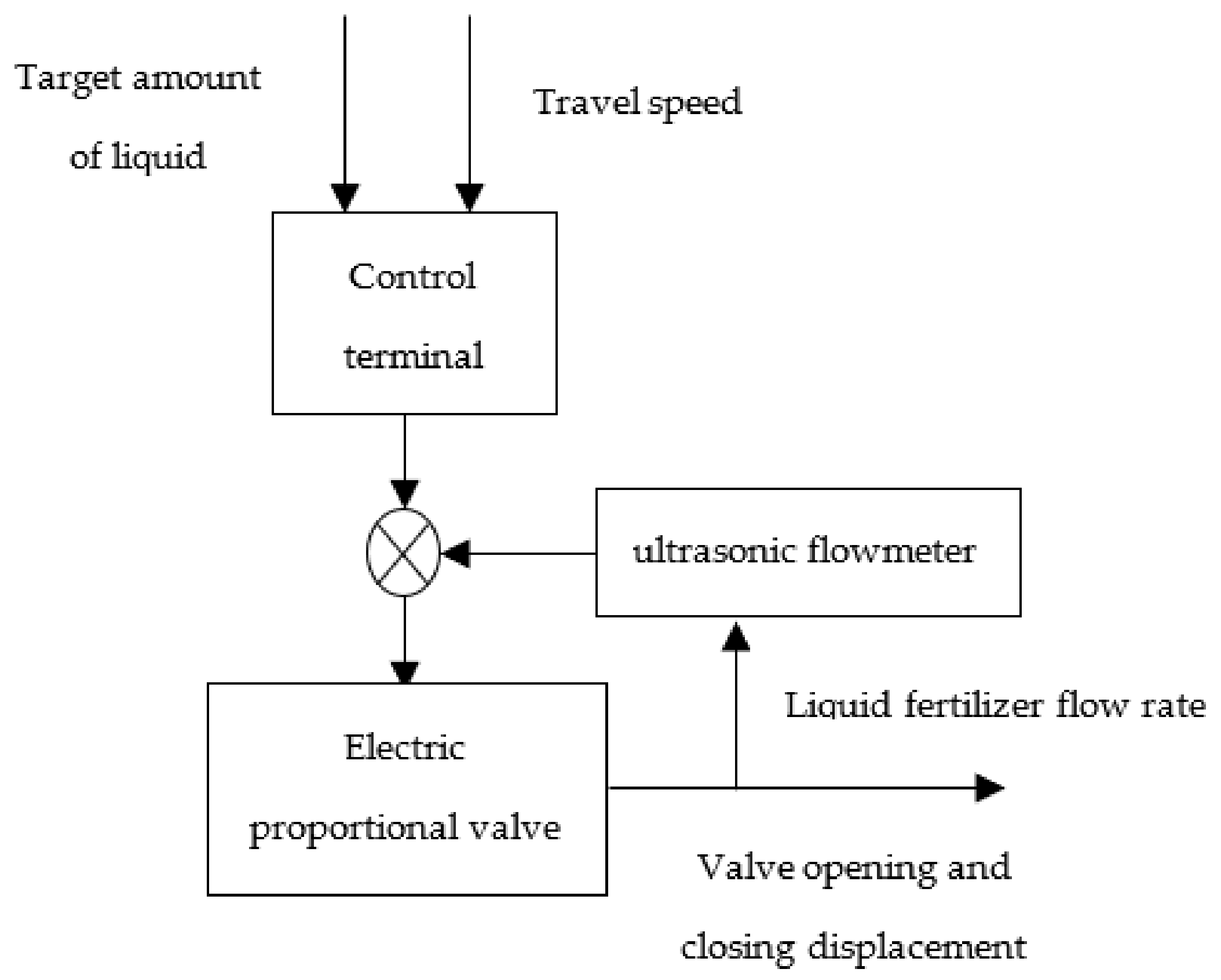
The operation of the main liquid manure spraying system decreased the response time of the operating system. This established the liquid manure spraying operating system transfer function. The liquid manure spreading input operating channel model was collected in real-time using an angular velocity sensor. The controller output the current signal to the solenoid valve after conversion. A solenoid valve was used to control valve opening. The final output of the system was the instantaneous current speed of liquid manure. Current speed was coupled back to the control system through the flowmeter in the flow chart of the operate channel, as exhibited in Figure 2. Finally, control via the inverse back-coupling closed cycle was conducted through the control system.
In the light of input/output relationships in the operating system flow chart, the system input/output relationships are presented (Equation (1)):
where V (L/min) is liquid manure volume exportation from the precision spray operating channel, F (q, v) is the transversion function, vehicle running speed is v(m/s), Q is the target fertilization amount input into the system according to the amount of liquid fertilizer used in corn fields in Tai’an, Shandong Province (q was set as 55 L/hm2), and W (m) is the width of fertilization. According to the vehicle conditions in this study, w = 6 m.
According to the liquid manure spraying operating channel in Figure 2, the system’s input feedback data were from the instantaneous discharge registration through the flowmeter. The current signal was the control system signal exported through the retroaction passageway. The control system switched signals and compared them with the target fertilizer amount and vehicle speed input to implement the inverse back-coupling control.
Thus, the control model feedback link use indicates Equation (2):
where t (s) is the delay time of preference transmission in the feedback link. The transfer function aleatory variable after the Laplace transform is S, and the transfer function inverse back-coupling chain is H.
The discharge monitoring of the operating channel via flowmeter in this study was real-time online. The retroaction latency of link time could be left out in the light of the actual hardware situation.
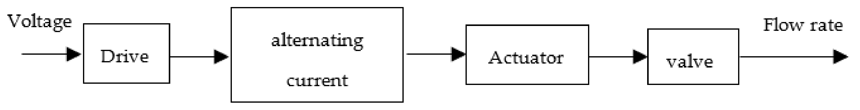
In the light of actual demand for a liquid manure precise spraying operating channel, the solenoid valve was our major control aim. We chose a Shanghai Kaiweixi Co. VB7200 solenoid valve. Figure 3 shows the signal control chart.
In Figure 3, propel module input/output signals were electricity semaphores. Transfer function was a ratio and delay segment. The relationship was as follows (Equation (3)):
where is the magnify quotient of the translator. as well as are current signal input/output with the propel module, respectively, and is the propel module’s transfer function.
Drive module current signal transmission delay (τ) was set to τ < 0.02 s. Therefore, τ was left out in the system, such that the propel module’s transfer function indicated a proportional sector [19].
The solenoid valve had a DC motor. The electricity signal was the dominant input signal. The angle of the electrical machinery’s axle was the output. The DC motor’s electro-circuit of semaphore control included an armature loop balance and induction of the rotor, as well as the balance of the axle couples of electrical system. Equation (4) demonstrates the balance equation:
Time (s) is expressed as . Entering electricity in the DC motor is (mA). The motor’s electromotance is expressed by E (V). The armature voltage is expressed by (V). Total armature resistance is expressed by (Ω). The armature’s inductance is expressed by (H). is the back electromotive force coefficient. The angle of electrical machinery’s axle is expressed by (°). The motor torque coefficient is displayed as . Motor load torque is displayed as (N⋯m, , where f is the friction coefficient). The rotational inertia of the rotor’s moment of inertia is expressed by (kg⋯m2). Finally, angular speed of the motor rotor is displayed as (rad/s).
The DC motor transfer function in the solenoid valve was obtained by transforming Equation (4) using a Laplace transformation, as shown in Equation (5):
where is the angle of the electrical machinery’s axle with the Laplace transform function. is the Laplace transform function of the motor input current, and is the motor’s transfer function. We can see Table 1 for simulation parameters [9].
The gear set was the main component of the reducer. The displacement output of the valve element was the axis speed of DC motor after deceleration. The valve element displacement, 0–18 mm, is expressed as X. The valve’s opening was translocation of the valve element.
The transmission relevance of decelerator input/output is expressed as the reduction ratio, which adopts the proportional dominant mode. The transfer function is expressed as follows (Equation (6)):
where the decelerator gear ratio is displayed as p. The lead of the drive rod is expressed with (mm). The spool traversed by the Laplace function is expressed by . The reducer transfer function is demonstrated with .
During this research, the flow and opening of the solenoid valve were linear under the same-pressure operating mode. Therefore, Equation (7) shows the relevance within flow and opening:
The flow as well as the valve opening’s transfer function is .
In Figure 3, the plant of the front path is guided by the solenoid valve. Equation (8) shows its transfer function:
where the transfer function of solenoid valve is defined by .
As can be seen from the control model as well as the functions of each control activity, in this research, Equation (9) is the closed–cycle retroaction control transfer function of the precision broadcast application control system:
The liquid manure spreading system’s dominant transfer function is .
2.4. PID Control Method
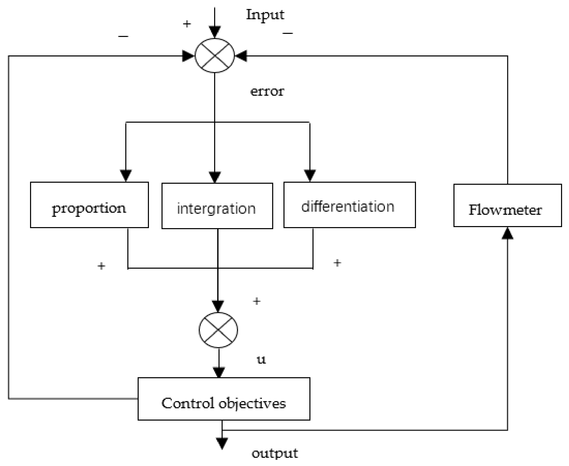
The PID control systematic is a classic control systematic. Figure 4 shows its operating system picture. The difference between the actual output signal of the controlled object and the given signal and tracking is the primary PID control method. The control rate (u) of the proportional (P), integral (I), and differential (D) systems was used as the main index for the analysis of the performance of liquid manure spraying. When the flowmeter feeds back the actual flow to the PID controller, the PID controller first reflects the difference between the actual flow and the demand flow in proportion. The output u (t) is directly proportional to the input deviation e (t), which can quickly reflect the deviation and thus reduce the deviation. Then, the function of the differential link can reflect the change trend (change rate) of the deviation signal, and can introduce an effective early correction signal into the system before the value of the deviation signal becomes too large, in order to speed up the action speed of the system and reduce the adjustment time. Finally, the integration link is used to eliminate the static error and improve the error-free degree of the system. The setting parameters of PID are provided by experience, through which the opening of the electromagnetic proportional regulating valve can be adjusted quickly. Through the feedback value of the flowmeter, the opening of the electromagnetic proportional valve is continuously adjusted to realize the PID control of liquid manure spraying. However, owing to the influence of nonlinearity and time delay in the process of liquid manure spreading, the precision of utilizing the classical PID dominant method to adjust liquid manure spreading is poor. Tracking variations in the application amount cannot be performed well with liquid manure spreading [20].
2.5. Devise of BPNN–PID Controller
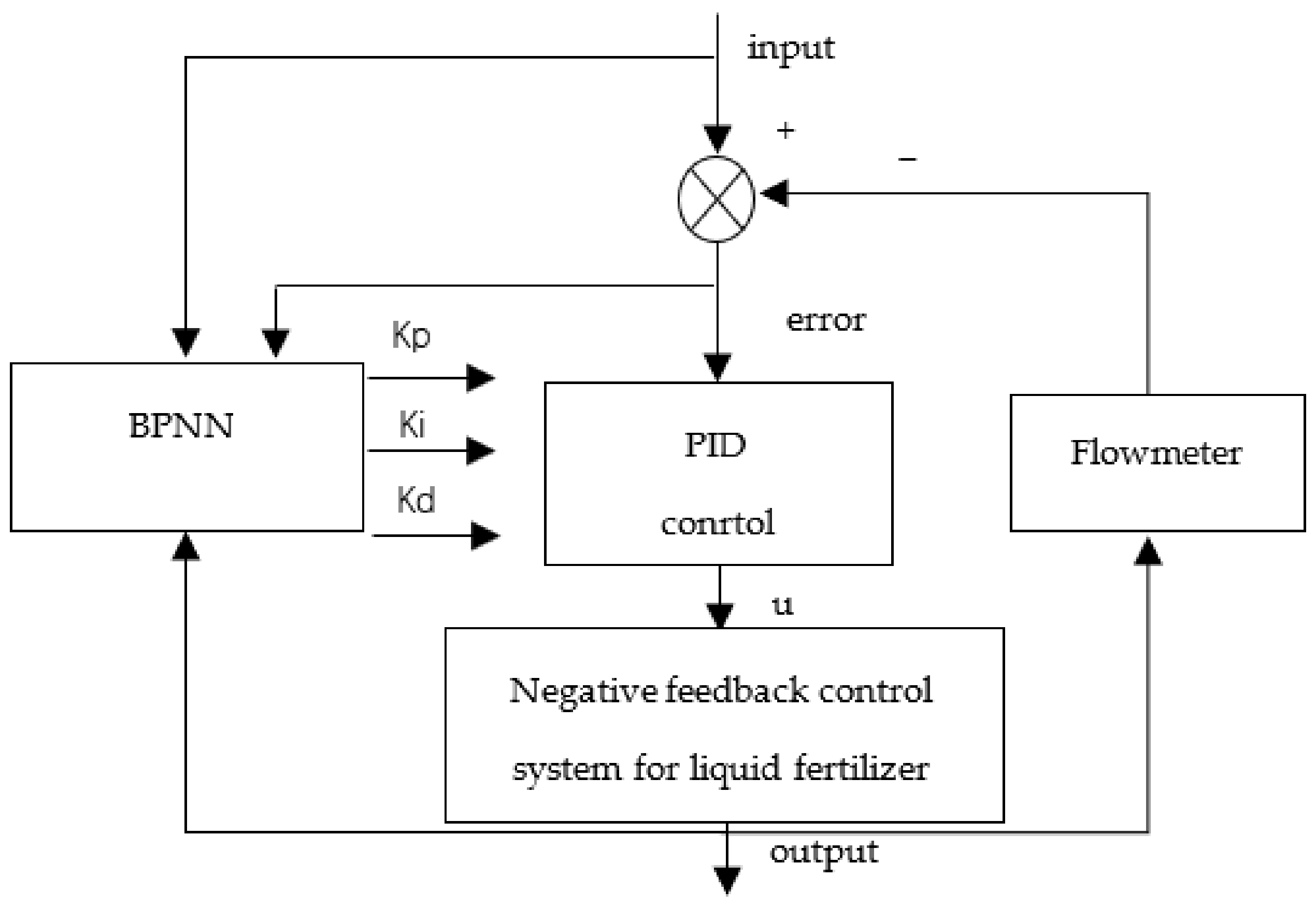
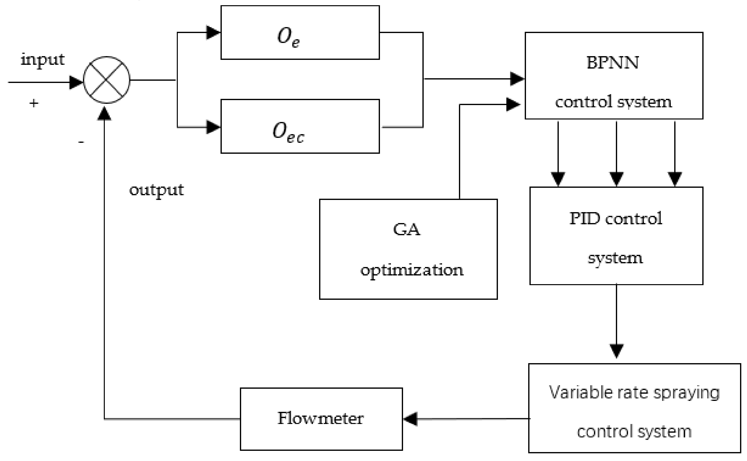
In this study, a BPNN–PID controller was designed according to the control requirements of an alternating–quantity scatter fertility control system for liquid manure. Figure 5 exhibits a flow chart of BPNN–PID control system.
The BPNN is a three–layer front-feed network. It includes three layers of network structure: the input layer, hidden layer, and output layer. The quantities of panel points in the import and export layers are decided by the dimensions of the input and output vectors, respectively. The concealed layer has a significant role in the ability as well as the composition of the system [21].
The BPNN–PID regulator was applied with three layers to define neurons with proportional, integral, and differential functions to integrate the regulation of PID control into the network. Through a teacher-free learning mode and online self-learning, adjustment could be carried out according to the control effect to ensure that the system performed well.
The first layer was the input layer, wherein the input was the preset fertilizer demand. The hidden layer was the second layer, wherein the entry was as follows (Equation (10)):
where is the hidden layer weight divisor. is the activation function in the hidden layer. The output layer was selected as third layer, with the following input and output: .
The output layer was the last layer, and the input and output can be seen from Equation (11):
Among , Li is the weight factor of the export layer. is the activation function of the output layer, wherein was selected.
After the BPNN–PID control outputs, KP, KI, and KD were determined; these were substituted for the bulking PID expression and calculated. Substitute PID control was used to memorize and maintain the system condition during above moments to minimize the impact of possible errors. Therefore, the optimal control signal was obtained by using incremental PID, as follows (Equation (12)):
where is the pilot signal spike, time is K, the scale factor is , the integration factor is , and the differentiation factor is .
2.6. Neural Network PID Control Algorithm Optimized by Genetic Algorithm
The study procedure of the BPNN mainly involves constantly adjusting the weight arguments of every network layer, followed by use of the weight ratio to count the optimum dominant arguments. Hence, the BPNN must study and constantly renew the weighting ratio array of every network layer.
2.6.1. Updating BPNN Weight Factor
In light of the BPNN study method, we delimit the target cost function L:
When the target cost function L was determined, a search was performed in the direction of the negative gradient. The objective was to minimize the target function L and add an inertial term to accelerate seek convergence to the global minima, as below:
where θ is the study rate and β is the ratio of inertia.
Thus, it was further concluded that the modified formula for the weight factor of the export layer of BPNN is:
According to over–calculation, the right formula for the hidden layer weight ratio was obtained as below:
where we set:
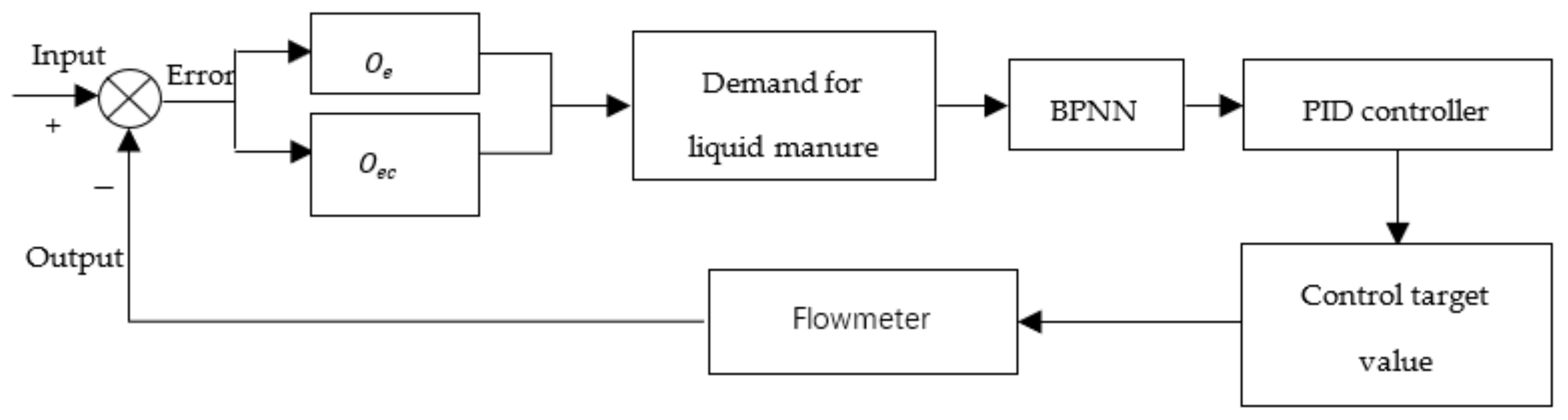
Therefore, the BPNN–PID control may be summarized as below: setting initialization of the three–layer system of BPNN arguments, together with inertia factor and study rate; using a BPNN control to process obtained error value; inputting the determined liquid fertilizer flow into the algorithm; and, after that, calculating the input/output of every layer via BPNN. Calculation of the three–layer arguments kp, ki, as well as kd of the PID control was performed using Expression (10). The export control signal is denoted by q (k). The systematic sustained renewal of q (k) along with the weight ratio of network on basis of the renew error value. A schematic of the control strategy is displayed in Figure 6.
2.6.2. BPNN–PID Algorithm Is Optimized using Genetic Algorithm
Recommending the Genetic Algorithm
A genetic algorithm screens individuals based on the chosen adaptation function combined with choice, intersection, and variation within the genetic process, retains those with good fitness value and eliminates those with inadaptable ones. The recent generation inherits information from the former generation and is better than the former generation. This loop was duplicated until the situation was met.
Optimizing BPNN Algorithm by Improving Genetic Algorithm
GA–BPNN–PID uses the genetic algorithm to optimize the weight and threshold of BPNN so that the optimized BPNN can better realize the function output. Although the GA–BPNN–PID control method is larger than the traditional method, the optimized BPNN weight and threshold can provide better control effect for the liquid manure spraying control algorithm. Both simulation and platform tests have verified that the algorithm has small overshoot, good stability, short rise time, and can better achieve the effect of precise spraying.
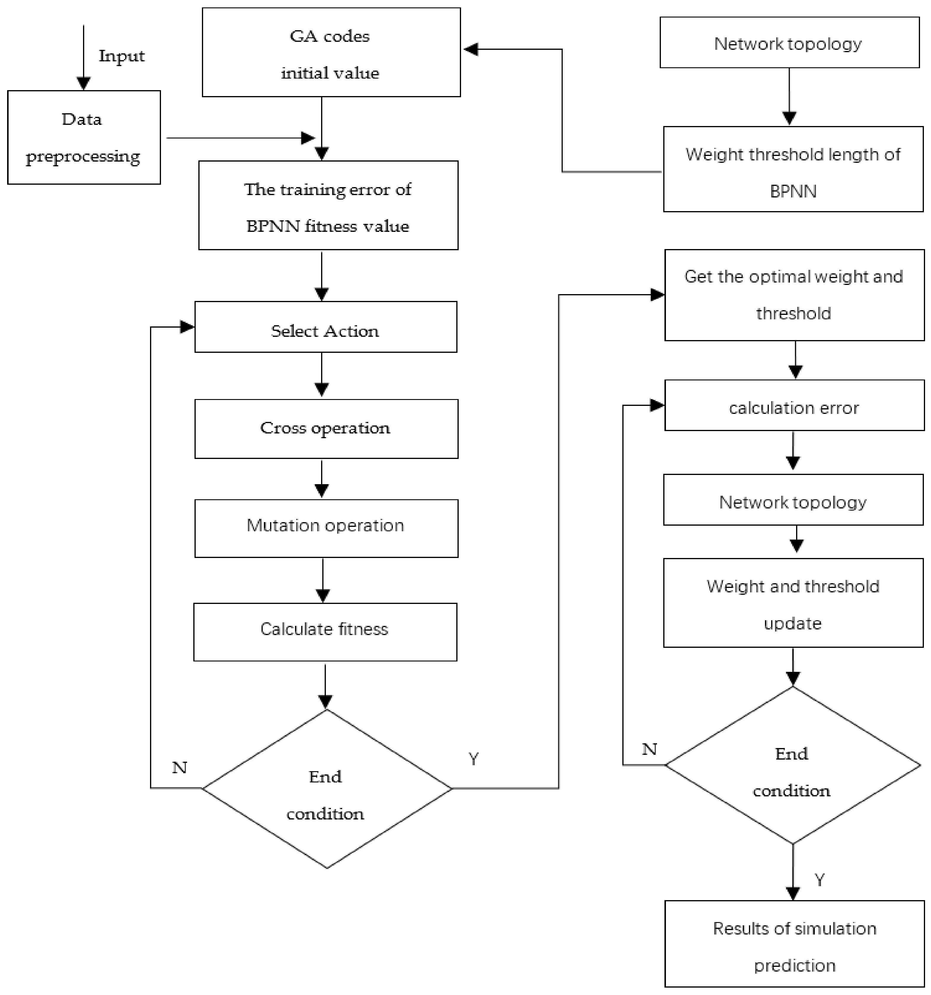
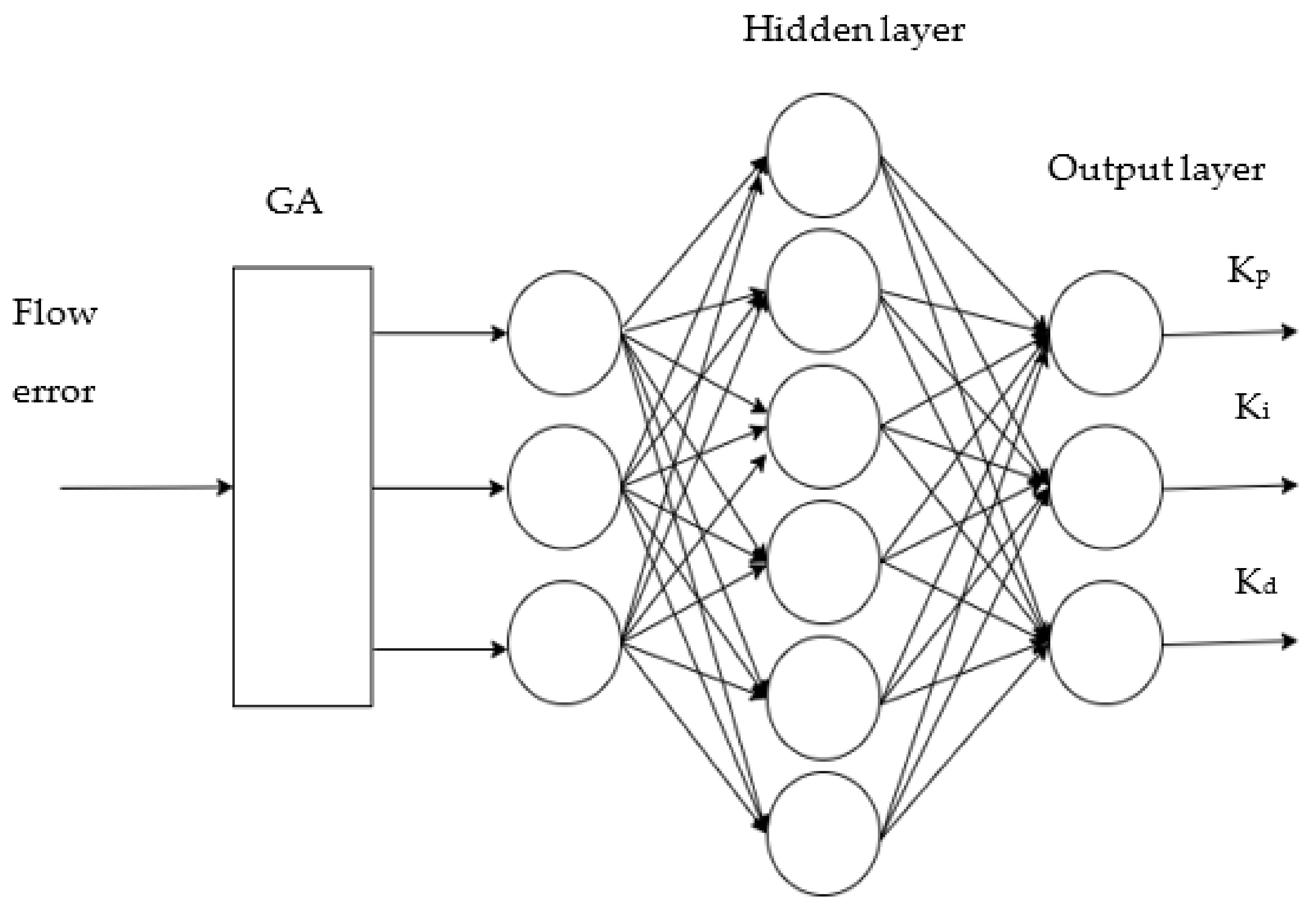
In this study, optimizing the BPNN has three parts: determination of the BPNN composition, optimization via genetic algorithm, then prediction by BPNN. The corresponding processes are illustrated in Figure 7. The structure of BPNN was determined according to the input and output parameters. In this study, the input was vehicle speed and the outputs were Kp, Ki, Kd. According to the above input and output data, we set the BPNN structure as 1-6-3, that is, the input layer had 1 node, the hidden layer had 6 nodes, and the output layer had 3 nodes, with a total of 19 weights and 9 thresholds. Therefore, the individual coding length of the genetic algorithm was 28. The BPNN prediction used a genetic algorithm to obtain the initial weight and threshold assignment of the optimal individual to the network. Finally, the prediction function was output after training. The GA–BPNN–PID structure diagram is shown in Figure 8.
The essential factors of BPNN optimized using genetic algorithm t included the initial population, fitness function, select action, crossover operator, and revisited mutations.
The genetic algorithm majorization main theory of the BPNN–PID dominant algorithm involved optimizing the initial value as well as the threshold of BPNN using a genetic algorithm, such that BPNN optimization could better forecast function export. Simultaneously, genetic algorithm optimization of the BPNN input state was used to reduce the network output and was insensitive to the system import, which was likely lag. The corresponding stages were as below:
- (1)
- Population initialization performed personality coding according to the actual amount or number coding. Every personality was the actual amount or number bunch. It was composed of four sections: link weight of import layer as well as hidden layer, the hidden layer threshold value, the link weight of the hidden layer and the export layer, and export layer threshold. When solving continuous optimization problems, the commonly used binary coding methods have a long code string, and the encoding and decoding operations take up more time. Therefore, this study did not use binary encoding and decoding. During this optimization, we used real numbers for coding. The real number used was the vehicle speed. The optimized algorithm could overcome the uncertainty of the continuous optimization process and improve the response time and accuracy of the optimized algorithm.
- (2)
- An individual obtained an initial weight value and threshold value in the BPNN. The output of the forecast machinery was predicted after training the BPNN on the training data. The absolute value of the error among the forecast export and expected output, as well as E, was compared with the personality fitness price Y. The count formula is as follows (Equation (18)):where n is the quantity of network export panel points, is the BPNN’s desired export of the ith panel point, is the forecast export of the ith panel point, and k is a ratio.
- (3)
- The choice manipulation of a genetic algorithm is the choice policy according to the fitness proportion. The choice percentage of every personality i was such that (Equation (19)):where is the fitness price of personality i. Before individual selection, the reciprocal of the fitness proportion was calculated. The factor is k, and N is the amount of the personality in the population.
- (4)
- In the light of optimizing the population initialization process, real number coding was adopted according to the individual; therefore, a real number crossover valve was adopted for the crossover operation. The overlapping operation of the k-th chromosome as well as c-th chromosome at position j is as below (Equation (20)):where d is a stochastic digit among (0–1).
- (5)
- In the mutation operation, the j-th gene of i-th personality was chosen with mutation. The mutation operation method was as below (Equation (21)):where is the top margin of gene , is the bottom margin of gene ; , is the stochastic digit, and f is the present iteration digit. are the maximum evolution times, and r is stochastic digit among [0–1]. Its control principle is exhibited in Figure 9.
2.7. Simulation Analysis of Spraying Control System
2.7.1. Modeling and Simulation of PID Control System
To achieve a control system model for liquid manure precise spraying, the classic PID control simulation variable spraying control system model of liquid manure was built using the Simulink simulation module in MATLAB software. The amplitude of import step signal was disabled by two. PID controller arguments were adjusted. The waveform of the system output was analyzed.
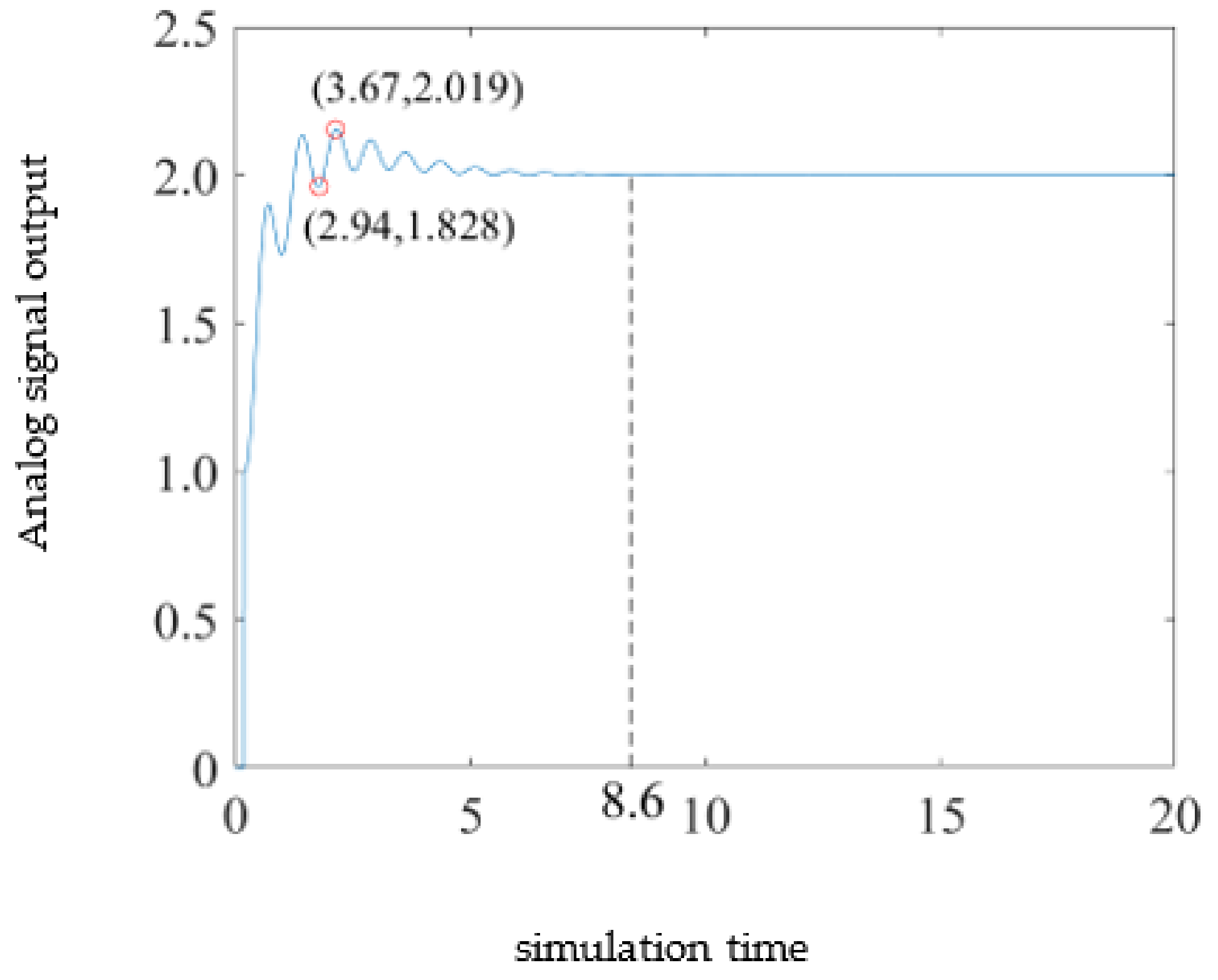
In the PID control simulation model, when t = 0, the import amplitude step signal was 2. Simulation time was disabled at 20 s. The KP, KI, and KD of PID control were set. Finally, the oscilloscope output a waveform. The simulated waveforms are displayed in Figure 10.
As shown in Figure 9, the model response time was 8.6 s, the overshoot was 0.019, and there was some oscillation before the system operation reached stability. Finally, KP = 42, KI = 0.51, and KD = 0.01 were selected according to the empirical trial method.
2.7.2. Modeling and Simulation of PID Control System
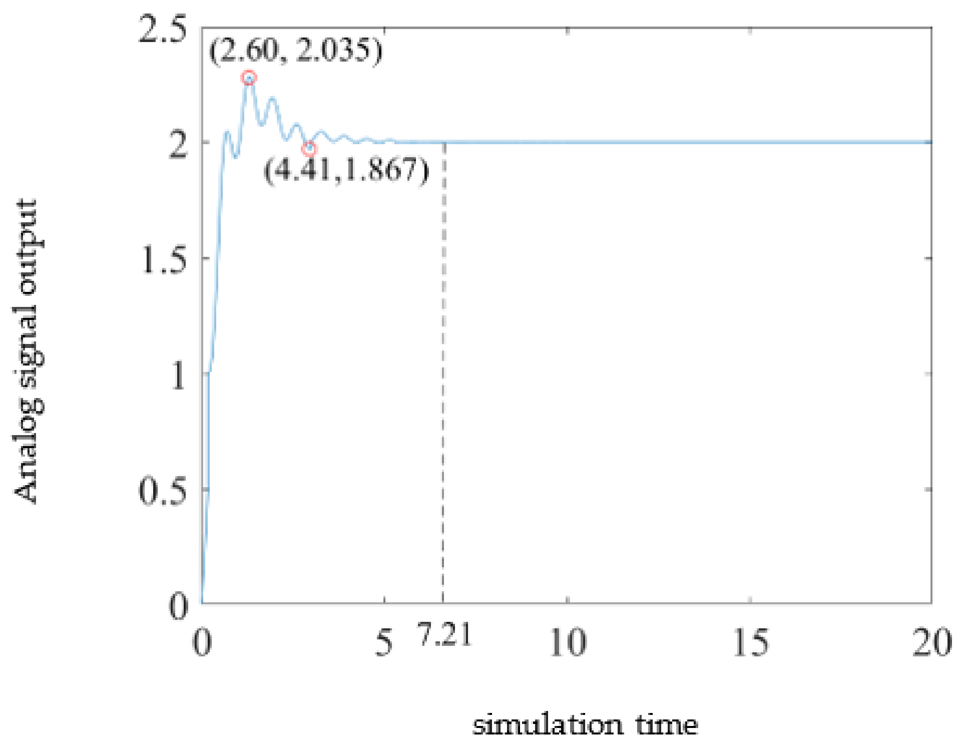
The simulation model of the fuzzy PID control system was established in the simulation module. The input signal was a saving signal of 2. The simulation process was as follows: input a step signal with amplitude of 2 at the time of t = 0, set the simulation time as 60 s, input variables of fuzzy controller as fuzzed error e (k) and error change rate ec (k). The fuzzy controller output the PID parameter compensation value after fuzzing and optimized the initial parameters through the compensation value. Finally, the control system simulation waveform was obtained [9]. The simulation waveform is shown in Figure 11. Figure 11 shows that the response time of fuzzy PID control was 7.21 s, and the overshoot was 0.035.
2.7.3. Modeling and Simulation of BPNN–PID Control System
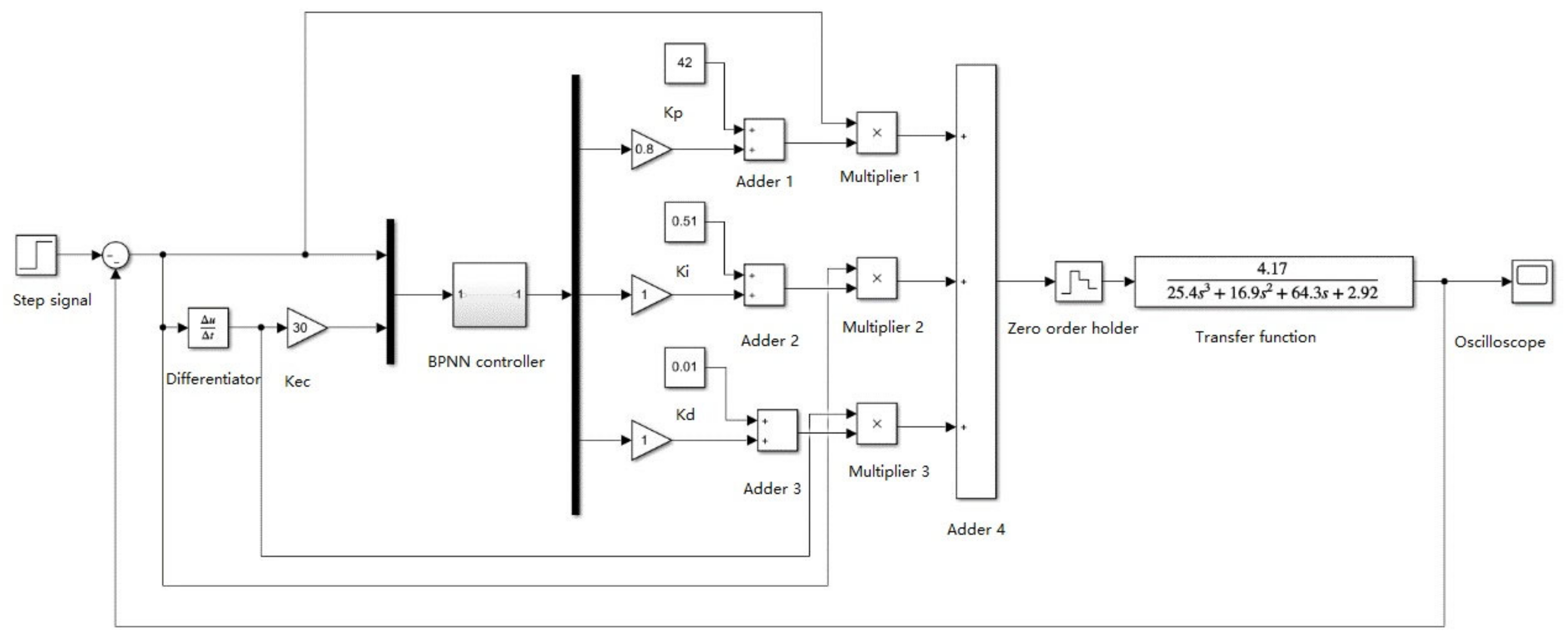
The simulation model of the BPNN–PID dominant system was established in the Simulink simulation module, and the input signal was also a step signal with an amplitude of 2. In the simulation process, the import amplitude step signal with an amplitude of 2 was time t = 0. Simulation time was disabled at 20 s. The input variables of the fuzzy regulator were the error e (k) and error rate of change ec (k) processed by the neural network, and the BPNN-PID regulator output compensation values of PID parameters after calculating KP, KI, and KD through BPNN. Initial parameters were optimized through compensation values, and the control system simulation waveform was obtained.
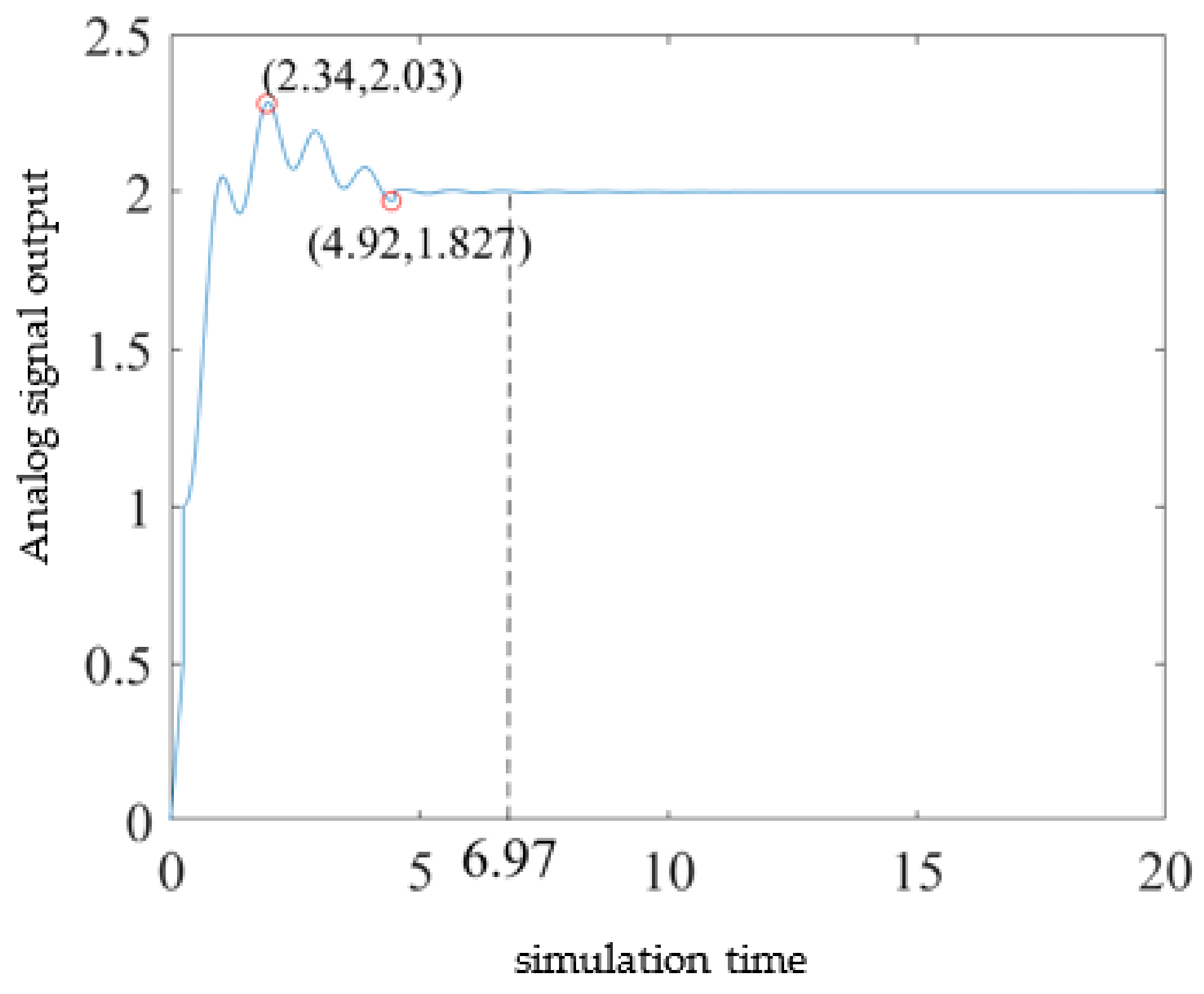
The built BPNN–PID control system model is displayed in Figure 12, while its simulation waveform is shown in Figure 13.
As shown in Figure 13, the reaction time of the BPNN–PID control was 6.97 s, the overshoot was 0.03, and there was some oscillation before the system ran stably. Compared with the classical PID control, the overshoot increased by 0.011, while the system response time decreased by 1.63 s. Compared with the fuzzy PID control, the overshoot decreased by 0.005, while the system response time decreased by 0.24 s.
2.7.4. Simulation Analysis of BPNN–PID Control System Optimized by Genetic Algorithm
A model-based alternating–quantity spraying dominant system of liquid manure genetic algorithm was programmed using MATLAB to optimize BPNN–PID control.
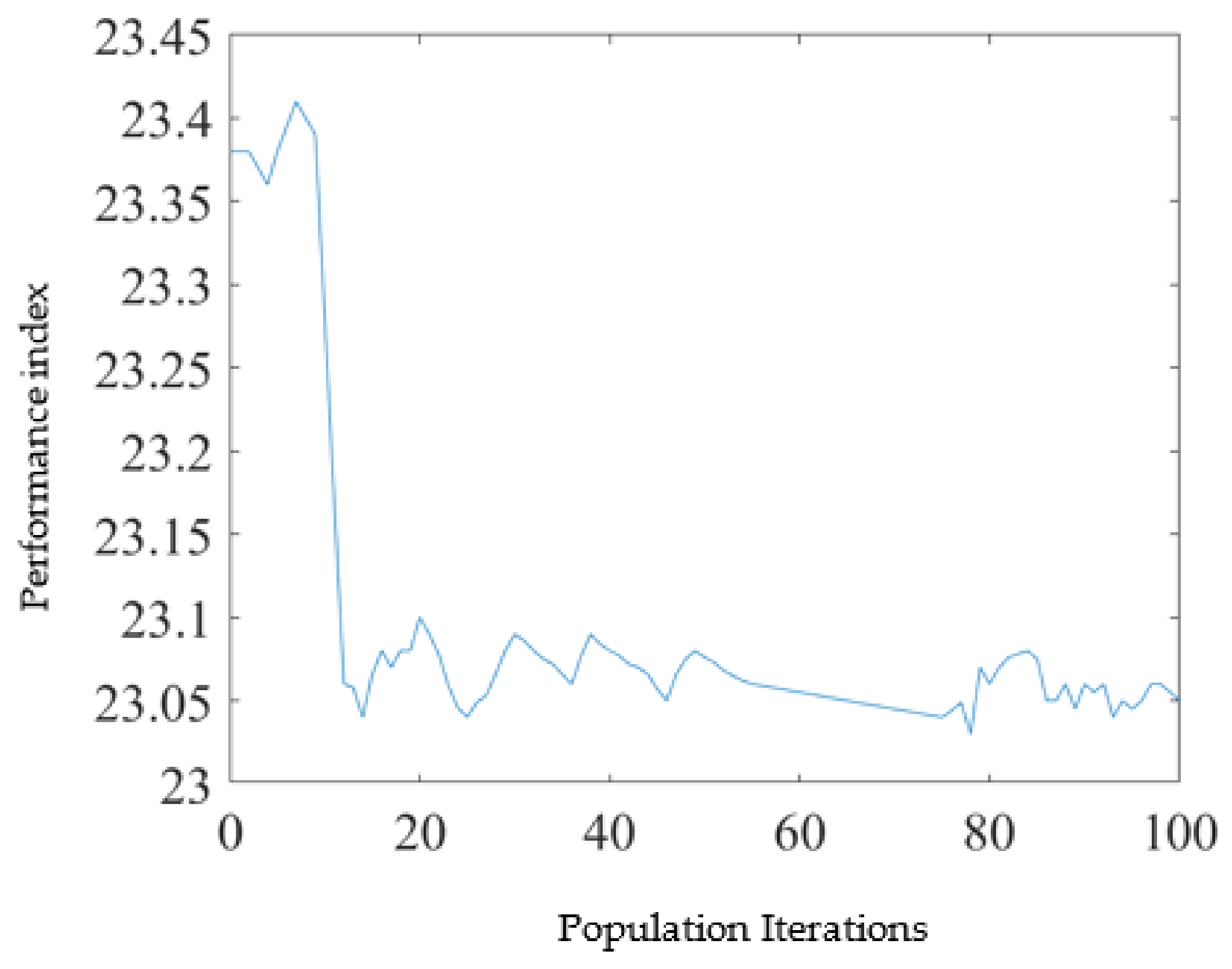
The absolute error integral criterion was used to judge the performance index of each generation of individuals optimized using the genetic algorithm. The optimization process was ended when the population iteration reached the required performance index. If the required index was not reached, the optimal individual in the last generation of the population was considered as the result of the control model simulation analysis.
The control system input a step signal with amplitude of 2, and then output the compensation values ΔKP, ΔKI, and ΔKD of the BPNN regulator corresponding to individual chromosomes before randomly generating the initial population. The individual chromosome in the population was optimized using the genetic algorithm operator, and the population was iterated to the maximum genetic algebra.
The iterative optimization process of the best individual of genetic algorithm is exhibited in Figure 14.
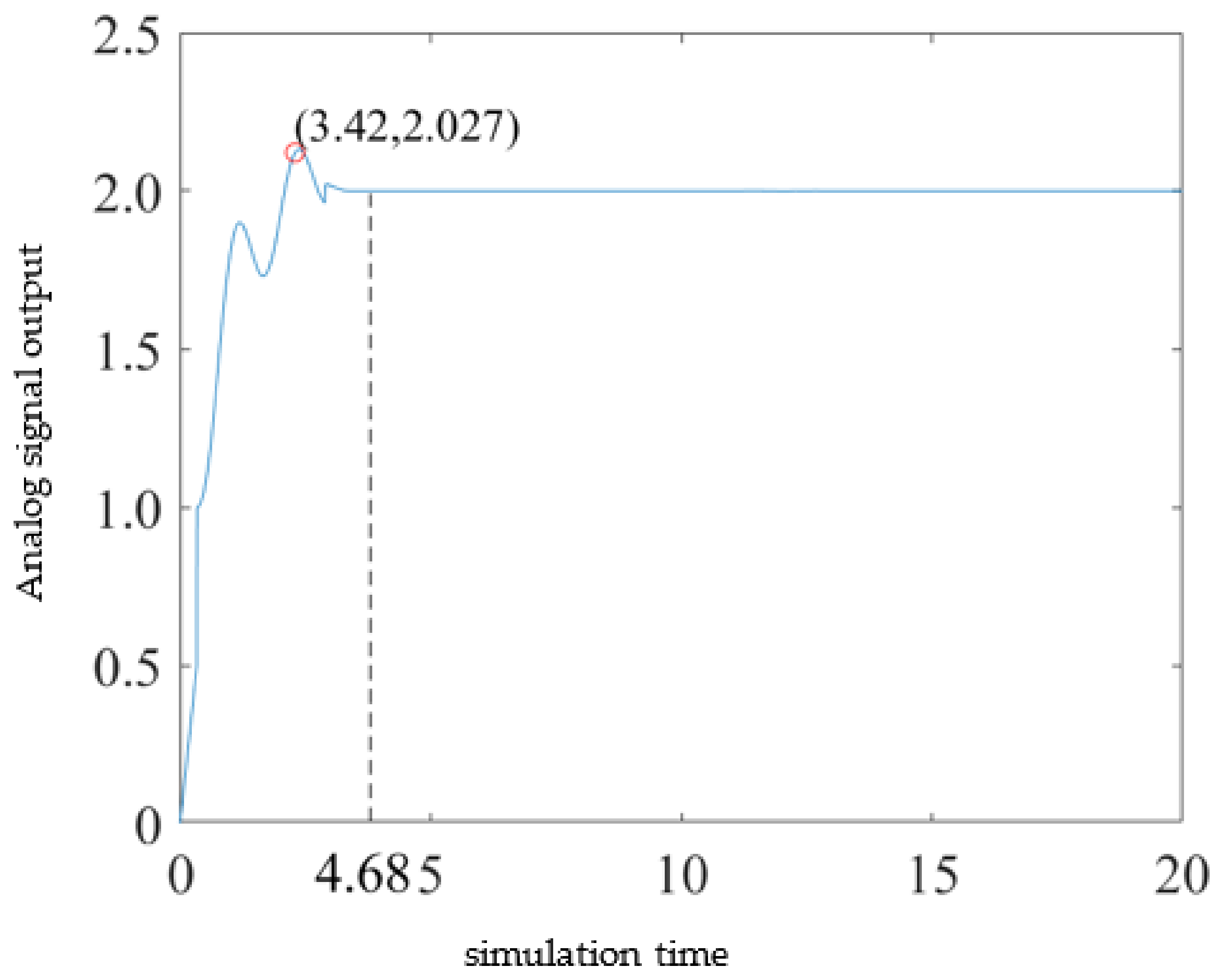
The optimized BPNN algorithm was imported into the PID controller, and the control model was simulated. The simulation results are exhibited in Figure 15.
As shown in Figure 15, for BPNN–PID control in view of genetic algorithm optimization, the response time of the system was 4.68 s and the overshoot was 0.027. After the system ran stably, a small disturbance was observed. Compared with the classical PID control, the overshoot increased by 0.008, while the response time was reduced by 3.92 s. Compared with the fuzzy PID control, the overshoot increased by 0.008, while the response time was reduced by 2.53 s. Compared with the BPNN–PID control, the overshoot was reduced to 0.003 and the response time decreased by 2.29 s. To summarize, the genetic–algorithm–optimized BPNN-PID control system had faster response, a smaller overshoot, and a better overall control effect.
3. Results
3.1. Test Materials and Platforms
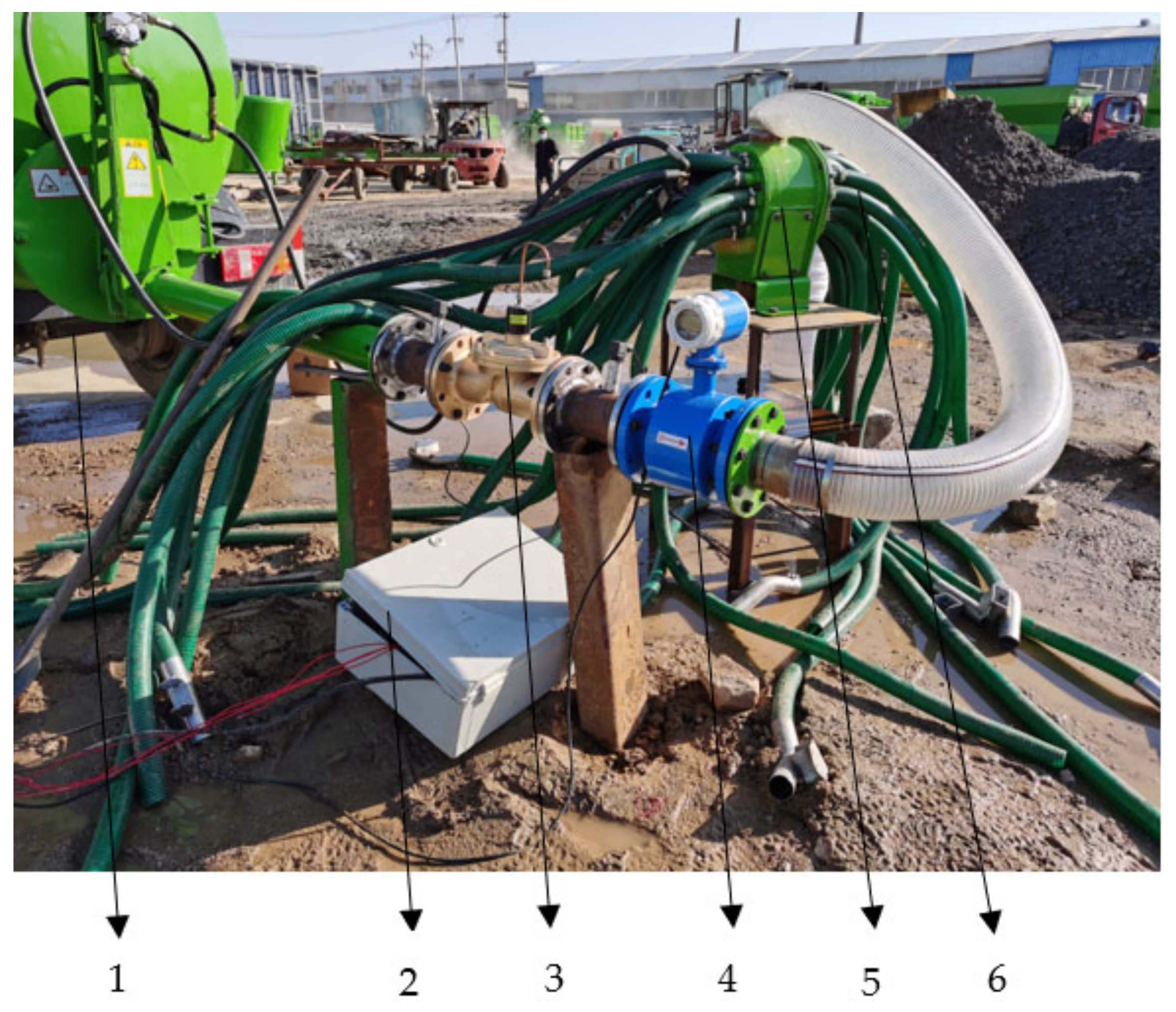
The variable application test of liquid manure was conducted in November 2021 and September 2022 at the test site of Tai’an Yimeite Co. Ltd. The test platform included a self-priming jet pump, monitoring and control via computer, electric proportional valve, flowmeter, distributor, and sprinkler pipe (Figure 16). The max lift of the self-priming jet pump was 15 m, the maximum absorption was 10 m, and the maximum flow was 81 L/min. The controller used the Siemens PLCS7–200 series, and the control software used the force control configuration software. The maximum diameter of the solenoid valve core was 18 mm. The maximum flow under 0.15 MPa pressure was 100 L/min.
The control object of the test was a proportional solenoid valve. The experiment material was clean water without suspended solids. The measurement and verification of the control accuracy of the flow rate of liquid manure distribution were carried out for classical PID control, fuzzy PID control, BPNN–PID control, and GA–BPNN–PID control.
The solenoid valve and control system of the experiment platform were powered by an onboard DC. The controller and actuator converted 48 V DC to 24 V DC by switching the power supply before sending them to the dominant system. The experiment platform was 1.8 m tall and 1.2 m broad.
3.2. Control Accuracy Analysis of Control System
In this study, the spreading accuracy of the control system was reflected by the flow error, flow control stability, and valve group response time under the condition of vehicle speed change. The open–shut processes of the solenoid valve were the main reasons for the fertilizer flow error. A degree of error was observed in the liquid supply of the self-priming jet pump, as well as the measurement of the flowmeter. Flowmeter error [22,23,24] was the main error. The potential main causes for the flow error are as follows: (i) the influence of sediment; (ii) the fluid contained many bubbles; (iii) the wave height being uneven during the flow of the liquid to be measured. In addition, the ultrasonic flowmeter was also possibly subject to external interference, such as the electromagnetic environment, which affects system accuracy.
In this control system, the flow error of the liquid manure mainly originated from the fluid. The absolute error of the fluid flow represents the difference between the reading value of the flowmeter and the actual flow, and the flow proportional error is the ratio of absolute error to actual flow.
Therefore, the flow error was calculated as follows (Equation (22)):
where Δ0 (L/min) is the absolute error of the system flow, Δ1 (%) is the relative error of the system flow, Vi (L/min) is the actual flow, and Vj (L/min) is the flow rate read by the flowmeter.
3.3. Experiment Results and Analysis
3.3.1. Control System Stability Experiment
The data measured by the ultrasonic flowmeter were transmitted to the upper computer through 4–20 mA current, while the actual liquid fertilizer flow of spraying and fertilization was measured using the test. We used the actual driving speed [25] of the traction liquid fertilizer spreader in the field. In the test, the vehicle speed was set to 1, 1.5, 2.0, and 2.5 m/s in the control system, and the flow relevant to every vehicle speed group was determined. Each flow group was measured 10 times, and the average value was taken after removing the highest and lowest values. Using a spraying amount of 300 L/hm2, the acknowledge fertilization quantities in the light of the above four different velocities were determined to be 10.8, 16.2, 21.6, and 27 L/min, according to Equation (1).
The system output flow was measured at four vehicle speeds. Six measurements were taken for each vehicle speed state. The duration of each measurement was 2 min. The mean value of the six measurements was considered with measurement flow of the velocity. Simultaneously, the absolute and proportional errors of every control system were noted. The experiment outcomes are listed in Table 2.
As shown in Table 2, the flow error of liquid manure controlled by classical PID was higher than that of BPNN–-PID control and GA–BPNN–PID. The PID flow control average relative error was 5.50%. The maximum absolute error was 0.91 L/min. The average relative error of the flow controlled by fuzzy PID was 3.67%. The maximum absolute error was 0.83 L/min. The average relative error of the flow controlled by BPNN-PID was 3.37%. The maximum absolute error was 0.83 L/min. The average relative error of GA–BPNN-PID was 0.97%. The maximum absolute error was 0.29 L/min. The experiment outcomes demonstrated that the relative error of the GA-BPNN-PID on the system flow control was the smallest. In comparison with PID control, the relative error was reduced by 4.53 percentage points, and compared with BPNN–PID control, the relative error was reduced by 2.4 percentage points. The control system exhibited the highest stability.
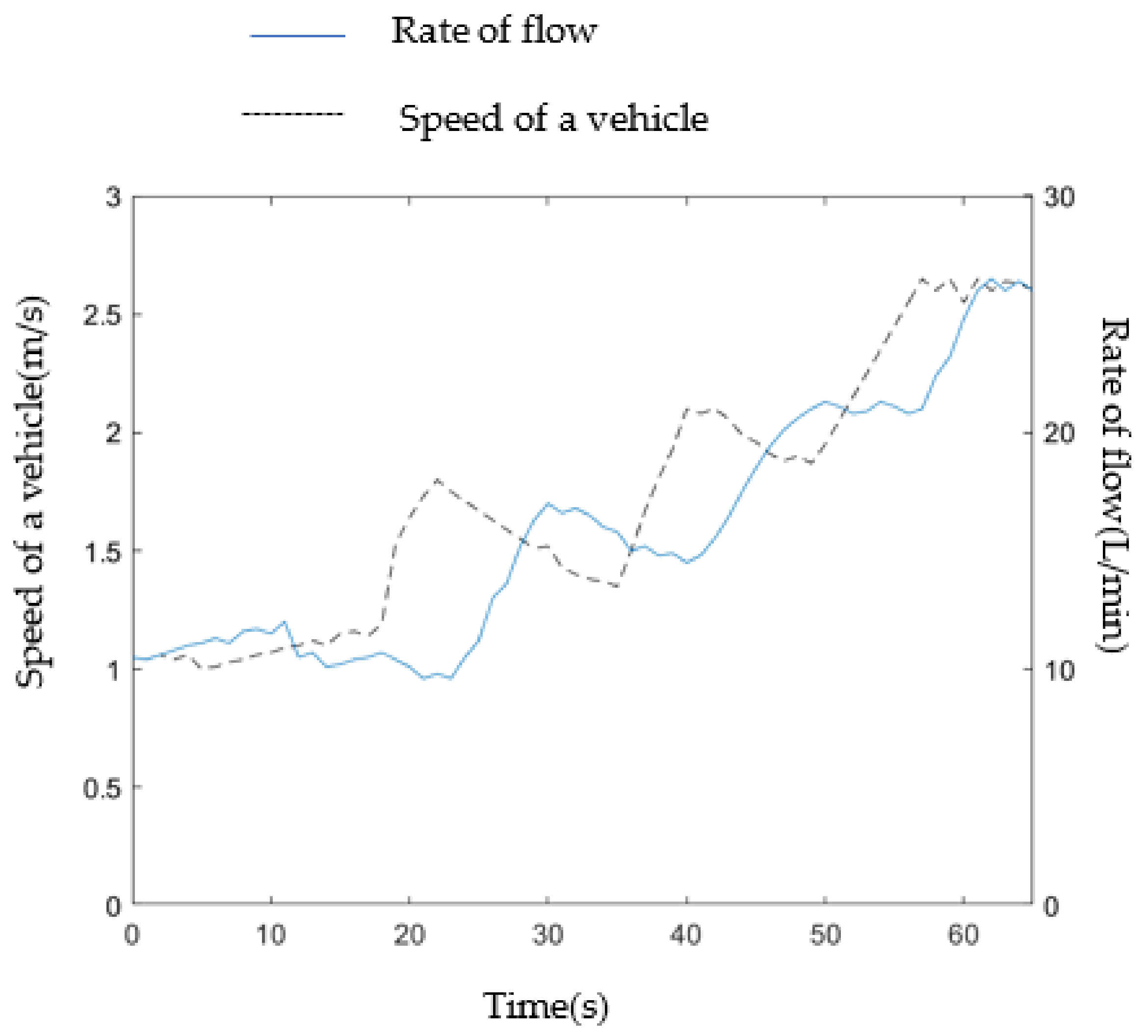
3.3.2. Variable Control Test
In the variable control test, a data acquisition card was used to collect the angular velocity sensor data. The square wave signal generated by the angular velocity sensor was used to calculate the vehicle speed. The gathered square wave signal was installed and stored through the programmable signal generator. In this test, a programmable signal generator was used to simulate the electrical signal when speed changed, and the classical PID, fuzzy PID control, BPNN–PID control, and GA–BPNN–PID control were used for variable control of liquid manure flow.
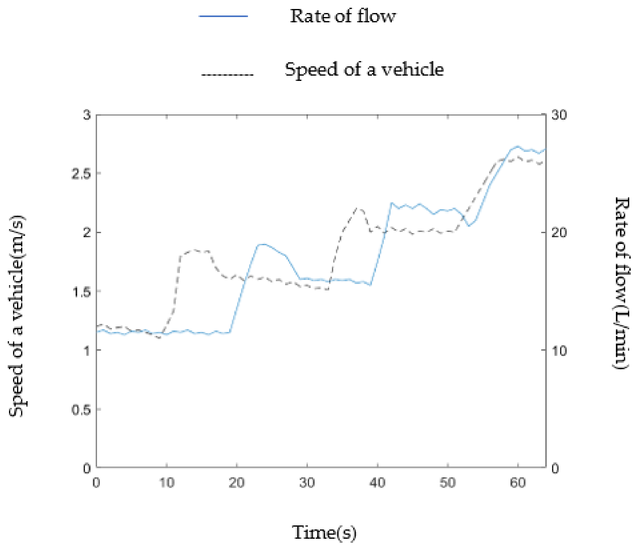
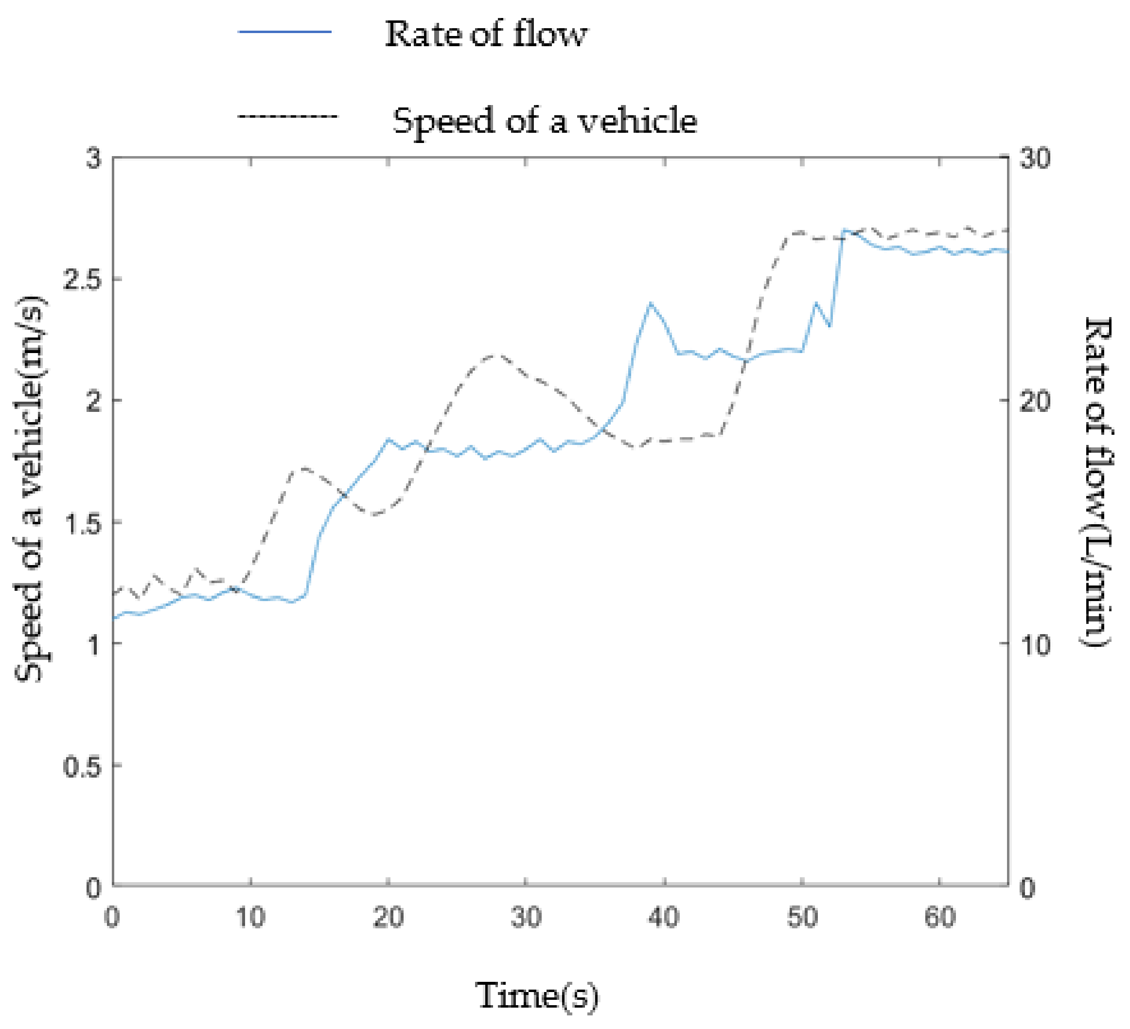
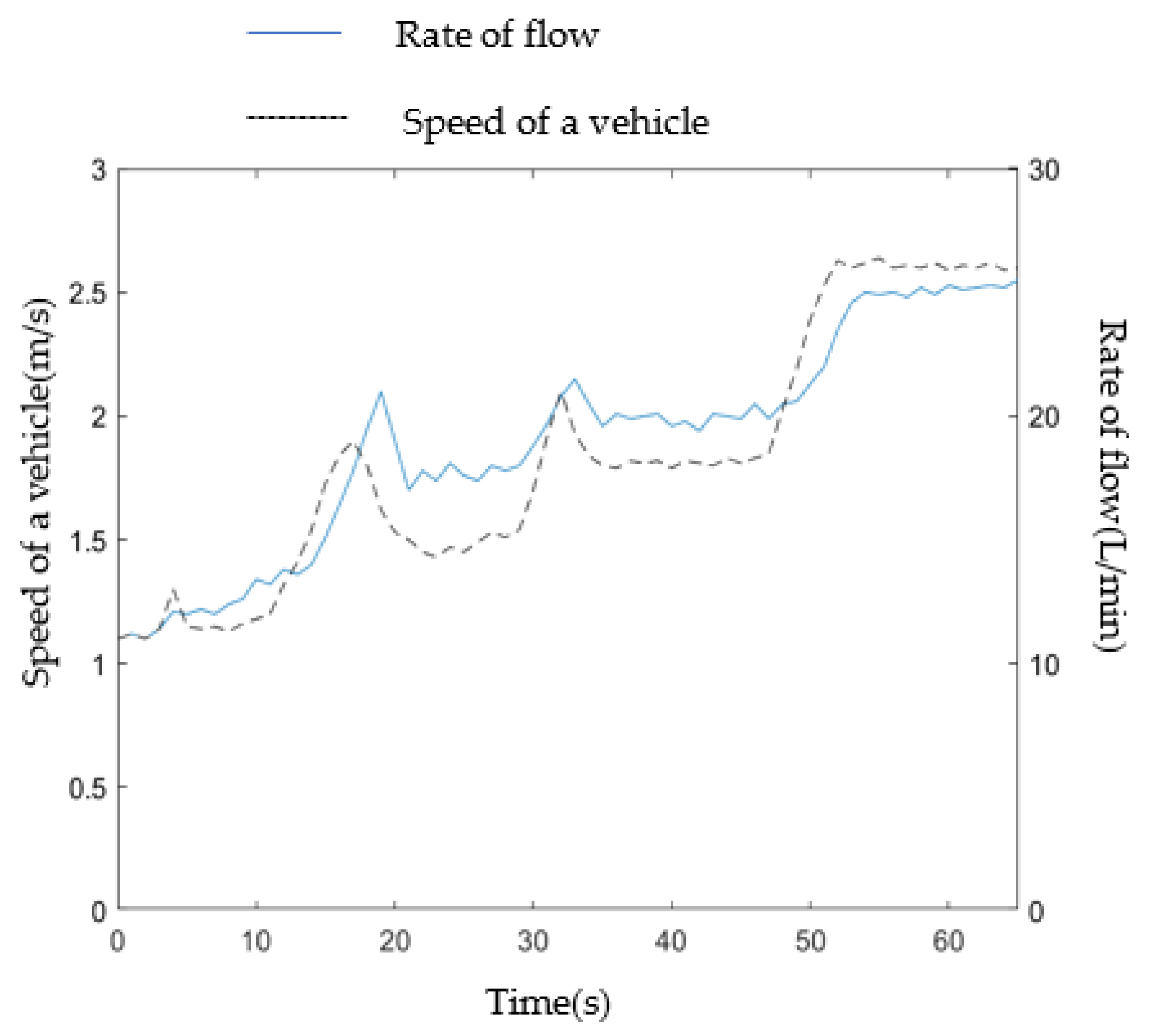
In this test, the discharge of liquid manure was determined using a flowmeter. Test data were noted after system stability. Test results for the liquid manure spreading control under the condition of vehicle speed change are shown in Figure 17, Figure 18, Figure 19 and Figure 20. During the spreading control system, the flow regulation’s average response time with the classical PID control was 5.02 s, the fuzzy PID control was 4.19 s, the BPNN-PID control was 3.97 s, and the GA–BPNN–PID control was 2.85 s. These results indicate that the actual response time of GA–BPNN–PID control was 2.17 s less than that of PID control, 1.34 s less than that of fuzzy PID control, and 1.12 s less than that of BPNN–PID control. The GA–BPNN–PID had the fastest response speed and better flow control stability.
4. Conclusions
In this study, spraying precision control technology was evaluated for use in a traction liquid manure variable spraying control system, and a control system model was built. Simulation analysis and tests were carried out for liquid manure flow control under the classical PID, fuzzy PID, BPNN–PID, and GA–BPNN–PID control modes. The following conclusions were drawn:
- (1)
- The GA–BPNN–PID optimized the dominant fertilizer system. This family has a variable-rate fertilizer-spraying control system model. GA–BPNN was used to optimize PID parameters, which enhanced the stability of the control system.
- (2)
- The negative feedback adjusting procedure of variable-rate liquid manure spraying control system was studied. The control system was modeled and simulated using MATLAB. The outcome shows that the response time for classical PID control to achieve stability was 8.6 s. The response time for fuzzy PID control to achieve stability was 7.21 s. The response time for BPNN–PID control to achieve stability was 6.97 s. The response time of GA–BPNN–PID control to achieve stability was 4.68 s. Thus, GA–BPNN–PID had the shortest response time and best stability.
- (3)
- Our experimental results show that for the variable distribution control system of liquid manure, the flow average relative error of liquid manure controlled by classical PID was 5.02%, the flow average relative error of liquid manure controlled by fuzzy PID was 3.37%, the flow average relative error of liquid manure controlled by BPNN–PID was 3.10%, and the flow average relative error of liquid manure controlled by GA–BPNN–PID was 1.07%. The practice response time of classical PID control was 5.02 s, the practice response time of BPNN-PID control was 3.97 s, 1.34 s less than that of fuzzy PID control, and the practice response time of GA–BPNN–PID control was 2.85 s. Compared with the classical PID control, the practice response time of GA–BPNN–PID control was reduced by 2.17 s, and the relative error was reduced by 3.95 percentage points. Compared with BPNN-PID control, the practice response time was reduced by 1.12 s, and the relative error was reduced by 2.03 percentage points. Therefore, the practice control effect of GA-BPNN-PID control was the best.
Taken together, the results presented in this study provide a reference for the fertilization control of maize in the field.
Author Contributions
This study was conceptualized by P.W. and M.C. Test setup was completed by P.W., B.X., A.W. and B.M. The software was designed by P.W. and A.W. B.X. and J.F. provided resources and P.W. curated the data. The original draft of the manuscript was prepared by P.W. and Y.C., B.M. reviewed and edited the manuscript. All authors have read and agreed to the published version of the manuscript.
Funding
This research was funded by the basic scientific research business expenses of CAAS, No. S202106-03, the Jiangsu Modern Agricultural Machinery Equipment and Technology Demonstration and Promotion Project (NJ2021-23), and the Jiangsu Modern Agricultural Machinery Equipment and Technology Demonstration and Promotion Project (NJ2022-26).
Institutional Review Board Statement
Not applicable.
Data Availability Statement
All relevant data presented in the article are stored according to institutional requirements and, as such, are not available on-line. However, all data used in this manuscript can be made available upon request to the authors.
Acknowledgments
We are grateful to Wei Zhao for his help in project management. We also thank Taian Yimeite Company for providing the experimental conditions for us to successfully complete this experiment.
Conflicts of Interest
The authors declare no conflict of interest.
Abbreviations
| PID | Proportion, integral, derivative |
| BPNN | BP neural network |
| BPNN-PID | BP neural network PID control system |
| GA-BPNN-PID | BP neural network PID control system optimized by genetic algorithm |
References
- Han, Y.; Jia, R.; Tang, H. Research status and development suggestions of precision variable-rate fertilization machine of the article. Agric. Eng. 2019, 9, 1–6. [Google Scholar]
- Ma, B.; Ming, J.C.; Ai, B.W.; Jing, J.F.; Zhi, C.H.; Bin, X.X. Working Mechanism and Parameter Optimization of a Crushing and Impurity Removal Device for Liquid Manure. Agriculture 2022, 12, 1228. [Google Scholar] [CrossRef]
- Jin, C.; Bin, Z.; Shu, J.Y. Research on present situation and the development countermeasures of variable rate fertilization technology in China. J. Agric. Mech. Res. 2017, 39, 1–6. [Google Scholar]
- Zhang, L.; He, Y.; Yang, H.; Tang, Z.; Zheng, X.; Meng, X. Analysis of the relationship between the development of liquid fertilizer machinery and modern agriculture. J. Chin. Agric. Mech. 2021, 42, 34–40. [Google Scholar]
- Meng, H.Q.; Xu, M.G.; Lü, J.L.; He, X.H.; Li, J.W.; Shi, X.J.; Chang, P.; Wang, B.R.; Zhang, H.M. Soil pH Dynamics and Nitrogen Transformations under Long-Term Chemical Fertilization in Four Typical Chinese Croplands. J. Integr. Agric. 2013, 12, 2092–2102. [Google Scholar] [CrossRef] [Green Version]
- Yang, X.J.; Yan, H.R.; Zhang, T.; Dong, X.; Sun, X. Development status and trend of dual-purpose self-propelled boom sprayer in paddy field and dry field in China. Agric. Eng. 2020, 10, 1–5. [Google Scholar]
- Zhu, D.L.; Ruan, H.C.; Wu, P.T.; Li, J.H.; Lu, L.Q. Remote fuzzy PID control strategy for fertilizer conductivity of water-fertilizer machine. J. Agric. Mach. 2022, 53, 186–191. [Google Scholar]
- Bai, Y.Q.; Xiong, K.H.; Zhi, C.W. Development of variable-rate spraying system for high clearance wide boom sprayer based on LiDAR scanning. Trans. Chin. Soc. Agric. Eng. 2020, 36, 89–95. [Google Scholar]
- Min, T.; Jin, B.B.; Jiang, Q.L. Variable rate fertilization control system for liquid fertilizer based on genetic algorithm. Trans. Chin. Soc. Agric. Eng. 2021, 37, 21–30. [Google Scholar]
- Zhuang, T.F.; Yang, X.J.; Dong, X.; Zhang, T.; Yan, H.R.; Sun, X. Research status and development trend of large self-propelled sprayer booms. Trans. Chin. Soc. Agric. Mach. 2018, 49 (Suppl. S1), 189–198. [Google Scholar]
- Chang, C.Y.; Hong, W.L.; Jin, H.; Guibin, C.H.; Caiyun, L.U.; Qingjie, W.A. Design and experiment of high-frequency intermittent fertilizer supply system based on PID algorithm. Trans. Chin. Soc. Agric. Mach. 2020, 51, 45–53. [Google Scholar]
- Li, T.; Jia, C.L.; Jing, L.W.; Zhang, B.; Lu, J. Design and experiment of bypass fertilizer-type water and fertilizer integrated automatic fertilizer applicator. Water Sav. Irrig. 2018, 11, 98–102. [Google Scholar]
- Yi, Y.; Feng, F.Z.; Xue, F.S. Design of self-propelled remote control spraying vehicle. Agric. Equip. Veh. Eng. 2021, 59, 46–49. [Google Scholar]
- Xiu, Y.X.; Bin, Z.; Ze, L.Z.; Shuran, S.; Zhen, L.; Hong, T.; Huang, H. Design and experiment of variable liquid fertilizer applicator for deep-fertilization based on ZigBee technology. J. Drain. Irrig. Mach. Eng. 2020, 38, 318–324. [Google Scholar]
- Saeys, W.; Engelen, K.; Ramon, H.; Anthonis, J. An automatic depth control system for shallow manure injection, Part 1: Modelling of the depth control system. Biosyst. Eng. 2007, 98, 146–154. [Google Scholar] [CrossRef]
- Guang, K.Z. Design and Experiment of Liquid Fertilizer Control System. Master’s Thesis, Northwest A&F University, Xianyang, China, 2018. [Google Scholar]
- Ji, C.Z.; Fan, F.M.; Ping, Z.; Shou, H.; Wen, J. Variable rate control and fertilization system of liquid fertilizer applicator based on electronic control unit. Soybean Sci. 2019, 38, 111–117. [Google Scholar]
- Qian, Z.; Zheng, Y.W.; Yu, B.Z.; Lei, Z.; Wei, J.; Haoran, W. Rapid-response PID control technology based on generalized regression neural network for multi-user water distribution of irrigation system head. Trans. Chin. Soc. Agric. Eng. 2020, 36, 103–109. [Google Scholar]
- Bi, P.; Zheng, J. Study on Application of Grey Prediction Fuzzy PID Control in Water and Fertilizer Precision Irrigation. In Proceedings of the 2014 IEEE International Conference on Computer and Information Technology (CIT), Xi’an, China, 11–13 September 2014; pp. 789–791. [Google Scholar]
- Wu, Y.; Li, L.; Li, S.; Wang, H.; Zhang, M.; Sun, H.; Sygrimis, N.; Li, M. Optimal control algorithm of fertigation system in greenhouse based on EC model. Int. J. Agric. Biol. Eng. 2019, 12, 118–125. [Google Scholar] [CrossRef] [Green Version]
- Zhou, R.; Zhang, L.; Fu, C.; Wang, H.; Meng, Z.; Du, C.; Shan, Y.; Bu, H. Fuzzy Neural Network PID Strategy Based on PSO Optimization for pH Control of Water and Fertilizer Integration. Appl. Sci. 2022, 12, 7383. [Google Scholar] [CrossRef]
- Le, Y.; Xiao, L.W.; Chun, L.Z. Correction of measurement deviation of turbine flowmeter. Energy Conserv. 2021, 2, 173–175. [Google Scholar]
- Xiu, L.Y. Error analysis in electromagnetic flowmeter. Ind. Des. 2017, 10, 141–142. [Google Scholar]
- Kang, X.Y.; Wei, W.; Bai, T.L. Discussion on the flow test method and development trend of the liquid flowing in the pipeline. China Met. Equip. Manuf. Technol. 2021, 56, 116–119. [Google Scholar]
- Jie, C. The application of PWM control in uniform and precise spraying for sprayer. J. Agric. Mech. Res. 2021, 43, 22–26. [Google Scholar]
Figure 1.
Structure diagram of fertilizer throwing control device: 1: tractor; 2: angular speed sensor; 3: pump; 4: liquid manure storage tank; 5: electric proportional valve; 6: flow meter; 7: liquid level meter; 8: monitoring and control by computer; 9: distributor; 10: sprinkler pipe.
Figure 1.
Structure diagram of fertilizer throwing control device: 1: tractor; 2: angular speed sensor; 3: pump; 4: liquid manure storage tank; 5: electric proportional valve; 6: flow meter; 7: liquid level meter; 8: monitoring and control by computer; 9: distributor; 10: sprinkler pipe.

Figure 2.
Control system diagram of liquid manure spreading.

Figure 3.
Signal control chart of solenoid valve.

Figure 4.
PID dominant method block diagram.

Figure 5.
BPNN–PID dominant system flow chart.

Figure 6.
Control schematic diagram of BPNN–PID regulator.

Figure 7.
Flow chart of GA–BPNN.

Figure 8.
GA–BPNN–PID structure diagram.

Figure 9.
GA–BPNN–PID control schematic diagram.

Figure 10.
Simulation waveform of PID control model.

Figure 11.
Simulation waveform of fuzzy PID control model.

Figure 12.
BPNN–PID control system model.

Figure 13.
Simulation waveform of BPNN–PID control model.

Figure 14.
Iteration results of optimal population of genetic algorithm.

Figure 15.
GA–BPNN–PID control system simulation waveform.

Figure 16.
Test platform. 1: pump; 2: monitoring and control via computer; 3: electric proportional valve; 4: flow meter; 5: distributor; 6: sprinkler pipe.
Figure 16.
Test platform. 1: pump; 2: monitoring and control via computer; 3: electric proportional valve; 4: flow meter; 5: distributor; 6: sprinkler pipe.

Figure 17.
Test results of liquid manure flow by PID control.

Figure 18.
Test results of liquid manure flow by fuzzy PID control.

Figure 19.
Test results of liquid manure flow by BPNN–PID control.

Figure 20.
Test results of liquid manure flow by GA–BPNN–PID control.


Table 1.
Simulation parameters.
| 0.51 | 4.32 × 10⁻³ | 1.02 × 10⁻⁴ | 0.27 | 0.3 | 1.527 × 10⁻⁴ |
Table 2.
Flow error of control system.
| Speed (m/s) | Calculated Flow Rate (L/min) | PID | Fuzzy PID | BPNN-PID | GA-BPNN-PID | ||||||||
|---|---|---|---|---|---|---|---|---|---|---|---|---|---|
| Actual Flow (L/min) | Absolute Error (l/min) | Relative Error (%) | Actual Flow (L/min) | Absolute Error (L/min) | Relative Error (%) | Actual Flow (L/min) | Absolute Error (L/min) | Relative Error (%) | Actual Flow (L/min) | Absolute Error (L/min) | Relative Error (%) | ||
| 1 | 10.8 | 11.38 | 0.58 | 5.37 | 11.26 | 0.46 | 3.7 | 11.14 | 0.34 | 3.17 | 10.87 | 0.07 | 0.67 |
| 1.5 | 16.2 | 17.09 | 0.89 | 5.49 | 15.57 | 0.63 | 3.9 | 16.78 | 0.58 | 3.56 | 16.35 | 0.15 | 0.92 |
| 2 | 21.6 | 22.88 | 1.28 | 5.93 | 22.42 | 0.82 | 3.7 | 22.39 | 0.79 | 3.65 | 21.86 | 0.26 | 1.21 |
| 2.5 | 27 | 28.39 | 1.39 | 5.2 | 27.91 | 0.91 | 3.4 | 27.83 | 0.83 | 3.09 | 27.29 | 0.29 | 1.06 |
Disclaimer/Publisher’s Note: The statements, opinions and data contained in all publications are solely those of the individual author(s) and contributor(s) and not of MDPI and/or the editor(s). MDPI and/or the editor(s) disclaim responsibility for any injury to people or property resulting from any ideas, methods, instructions or products referred to in the content. |
© 2023 by the authors. Licensee MDPI, Basel, Switzerland. This article is an open access article distributed under the terms and conditions of the Creative Commons Attribution (CC BY) license (https://creativecommons.org/licenses/by/4.0/).
Share and Cite
MDPI and ACS Style
Wang, P.; Chen, Y.; Xu, B.; Wu, A.; Fu, J.; Chen, M.; Ma, B. Intelligent Algorithm Optimization of Liquid Manure Spreading Control. Agriculture 2023, 13, 278. https://doi.org/10.3390/agriculture13020278
AMA Style
Wang P, Chen Y, Xu B, Wu A, Fu J, Chen M, Ma B. Intelligent Algorithm Optimization of Liquid Manure Spreading Control. Agriculture. 2023; 13(2):278. https://doi.org/10.3390/agriculture13020278
Chicago/Turabian StyleWang, Pengjun, Yongsheng Chen, Binxing Xu, Aibing Wu, Jingjing Fu, Mingjiang Chen, and Biao Ma. 2023. "Intelligent Algorithm Optimization of Liquid Manure Spreading Control" Agriculture 13, no. 2: 278. https://doi.org/10.3390/agriculture13020278
Note that from the first issue of 2016, this journal uses article numbers instead of page numbers. See further details here.