
Smart Weather Data Management Based on Artificial Intelligence and Big Data Analytics for Precision Agriculture

 , , , ,
  and
and
Abstract
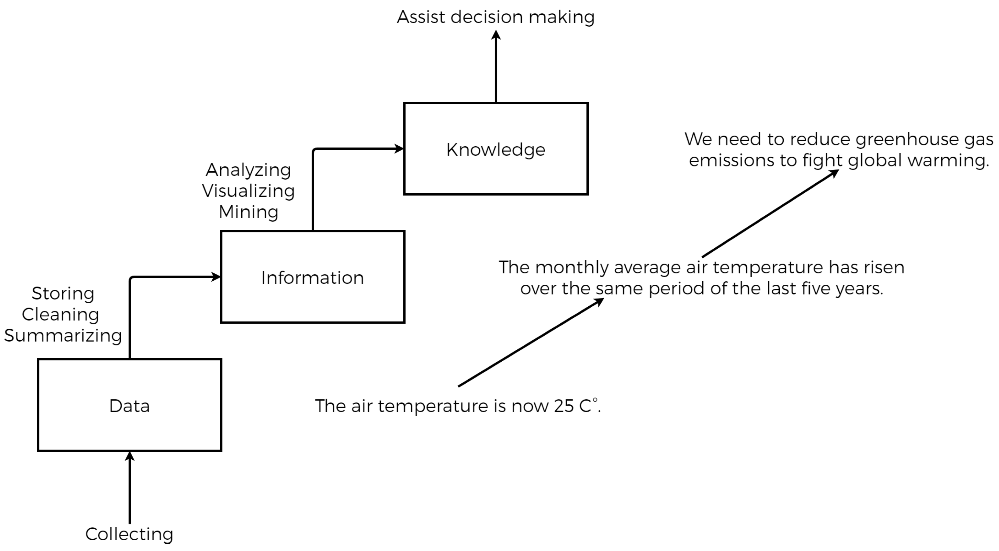
:1. Introduction
2. State of the Art
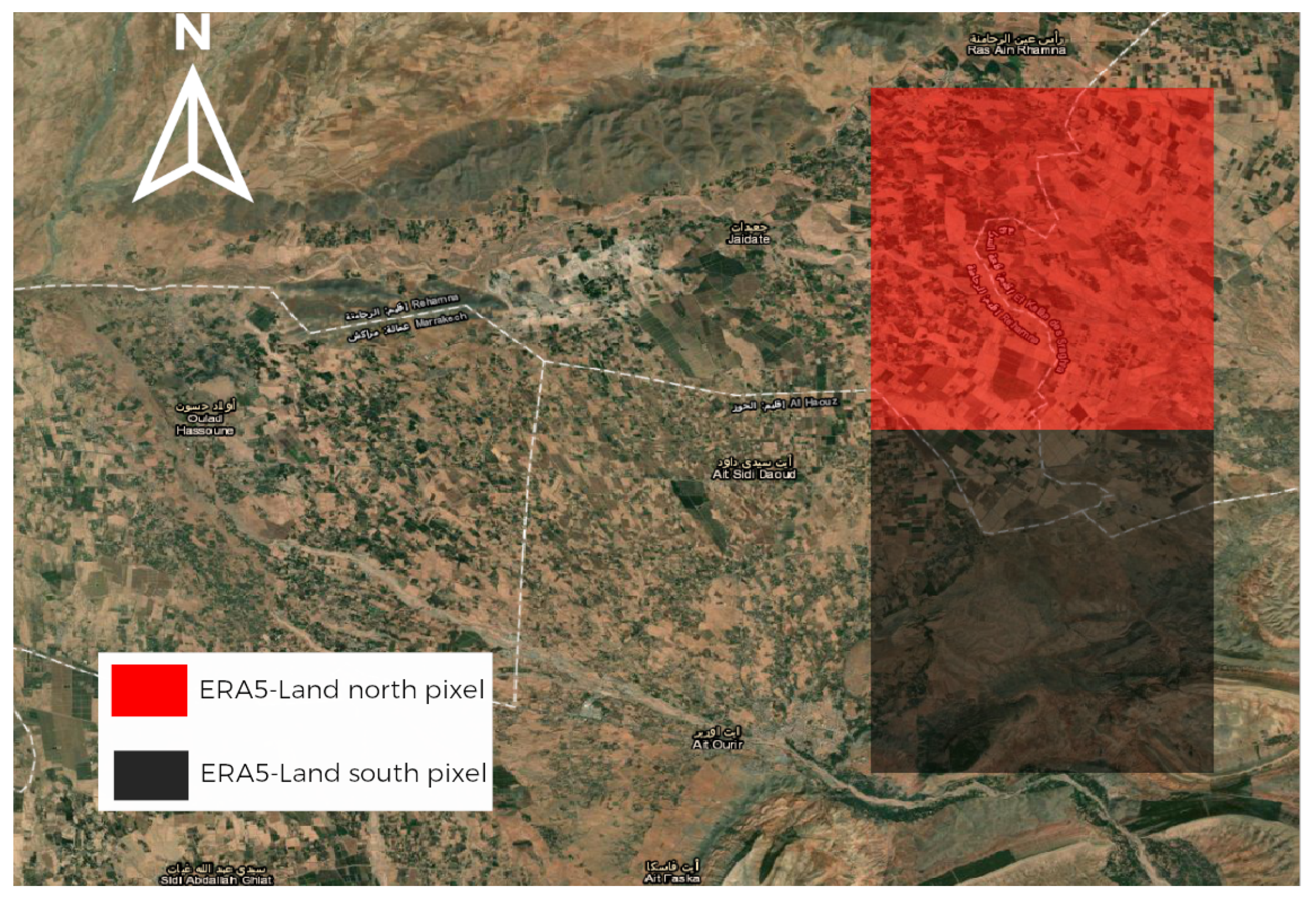
3. Study Area
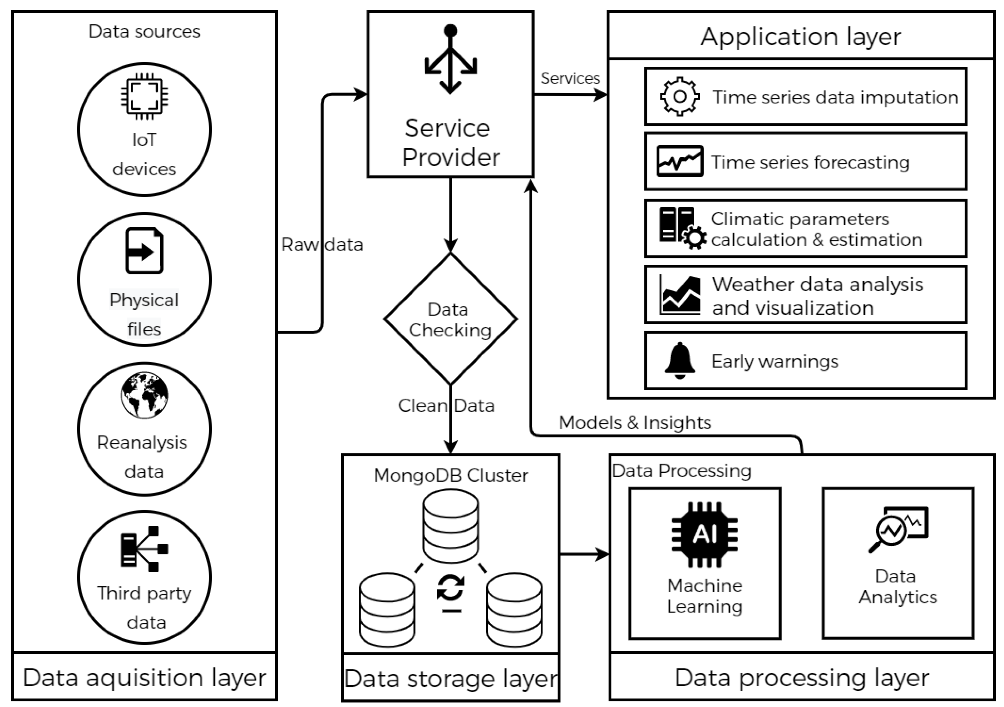
4. System Architecture
4.1. Data Acquisition Layer
4.1.1. Weather Station Data
- Incoming solar radiation using (Kipp and Zonen CM5 Pyranometer, Delft, The Netherlands).
- Air temperature in Kelvin, relative humidity (R3_Hr, as a fraction between 0 and 1) and vapor pressure by using (HMP45C, Vaisala, Helsinki, Finland).
- Wind speed using (A100R Anemometer, R.M. Young Company, Traverse City, MI, USA).
- Rainfall using (FSS500 Tipping Bucket Automatic Rain Gauge, Campbell Scientific Inc., Logan, UT, USA).
4.1.2. ERA5-Land Reanalysis Data
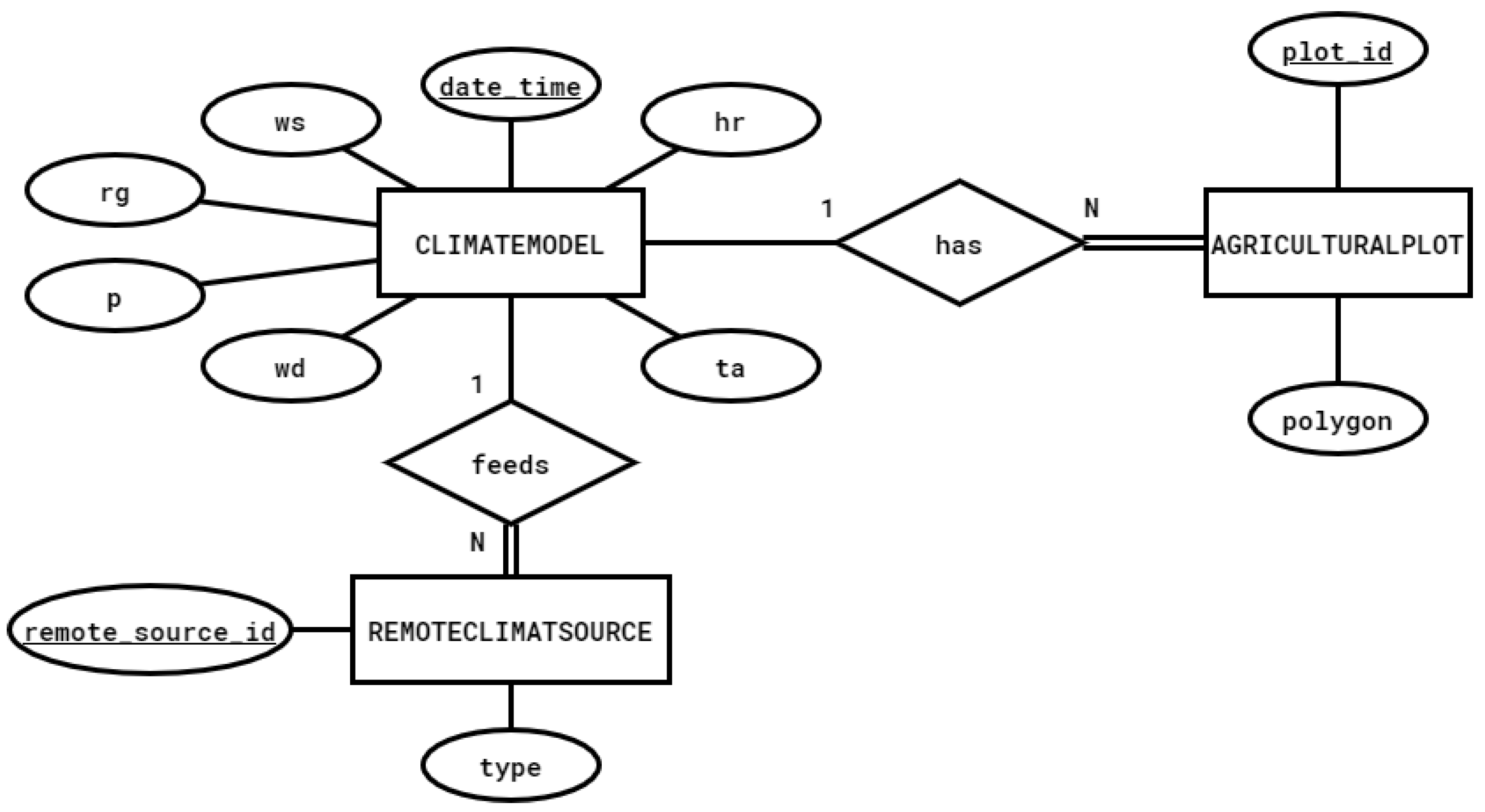
4.2. Data Storage Layer
4.3. Data Processing Layer
4.3.1. Statistical Models
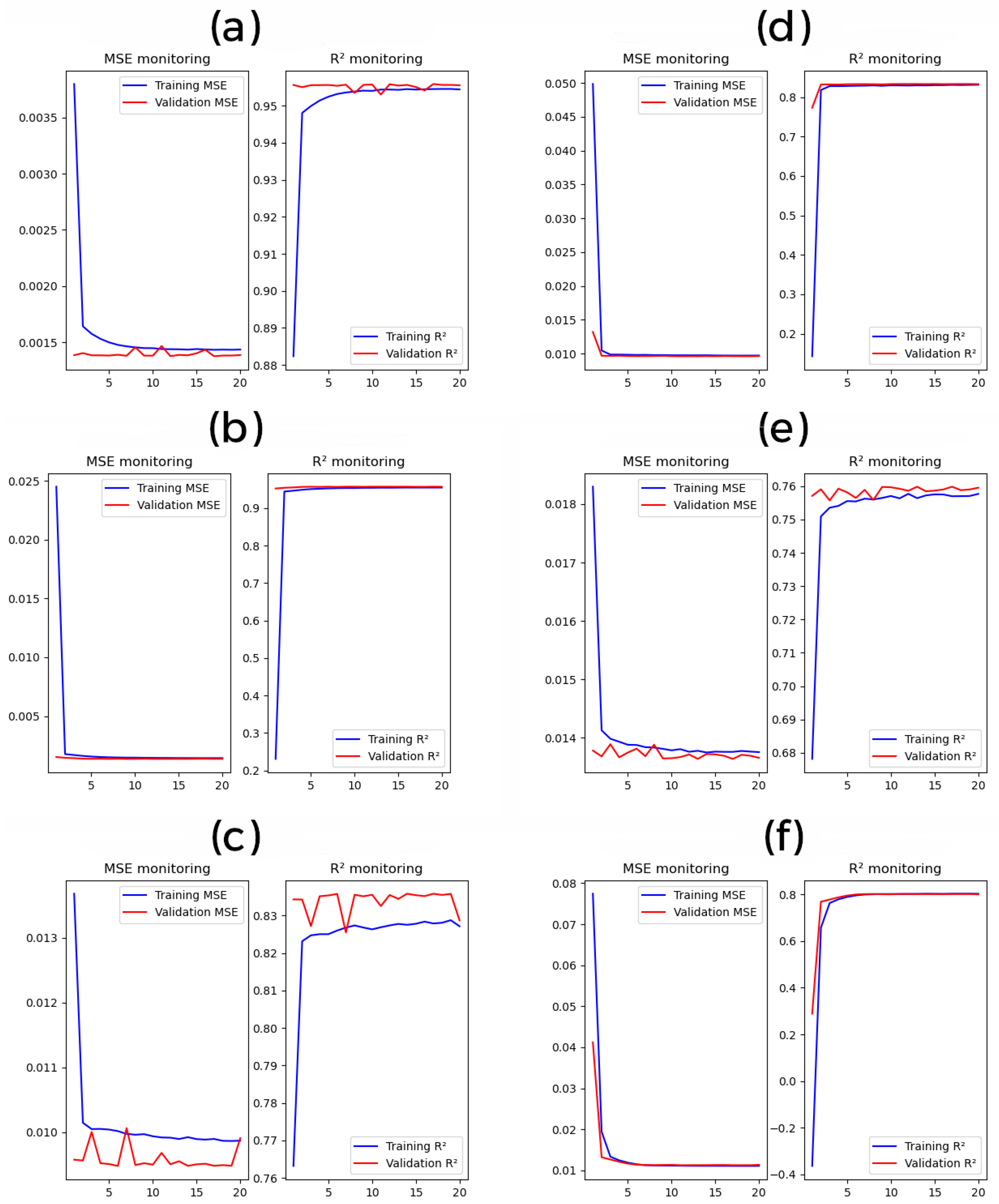
4.3.2. Machine Learning Models
4.3.3. Deep Learning Models
4.4. Application Layer
4.4.1. Time Series Data Imputation Service
- Deletion: Deleting rows or columns with missing values will remove this unwanted type of data from our dataset, but it may drastically reduce the size of the dataset, especially in the context of data scarcity.
- Imputation in time series data: In the case of a time series with a trend and seasonality, missing data can be replaced using seasonal adjustment, such as using the data from the same period of the previous year, which is the case for most weather data. However, this method may not be as efficient due to changes in weather patterns around the world. In contrast, if the time series do not present a trend or a seasonality, it can be treated the same way as imputation for a normal dataset.
- Imputation in normal datasets: Replacing it using statistical measures of central tendencies such as the mean, median, or mode of a given window of data that require some assumptions about the distribution type of the data to be efficient.
- a. Exploratory data analysis
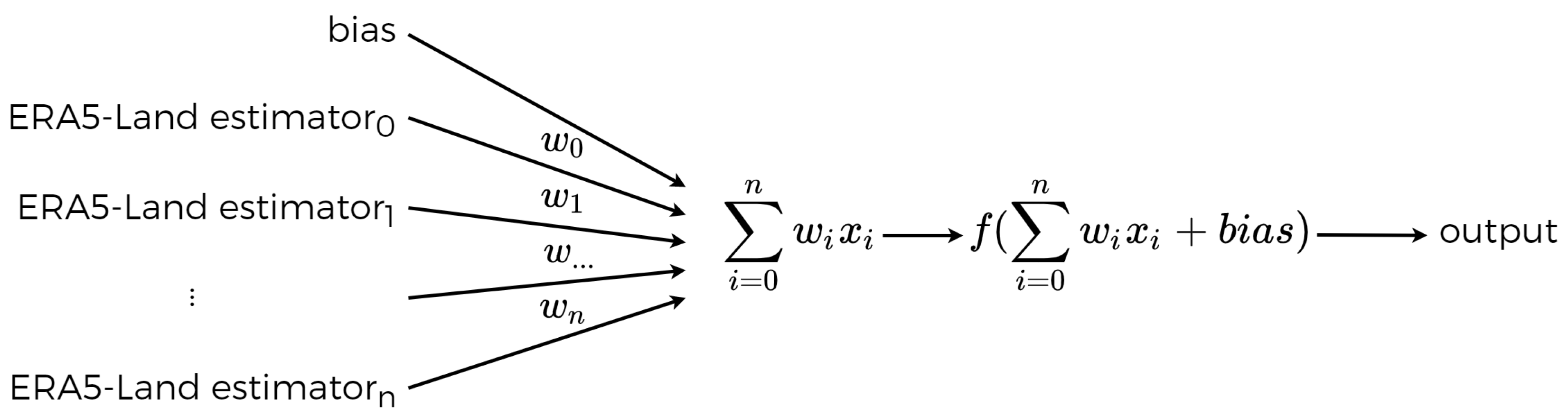
- b. Feed Forward Neural Network (FFNN):
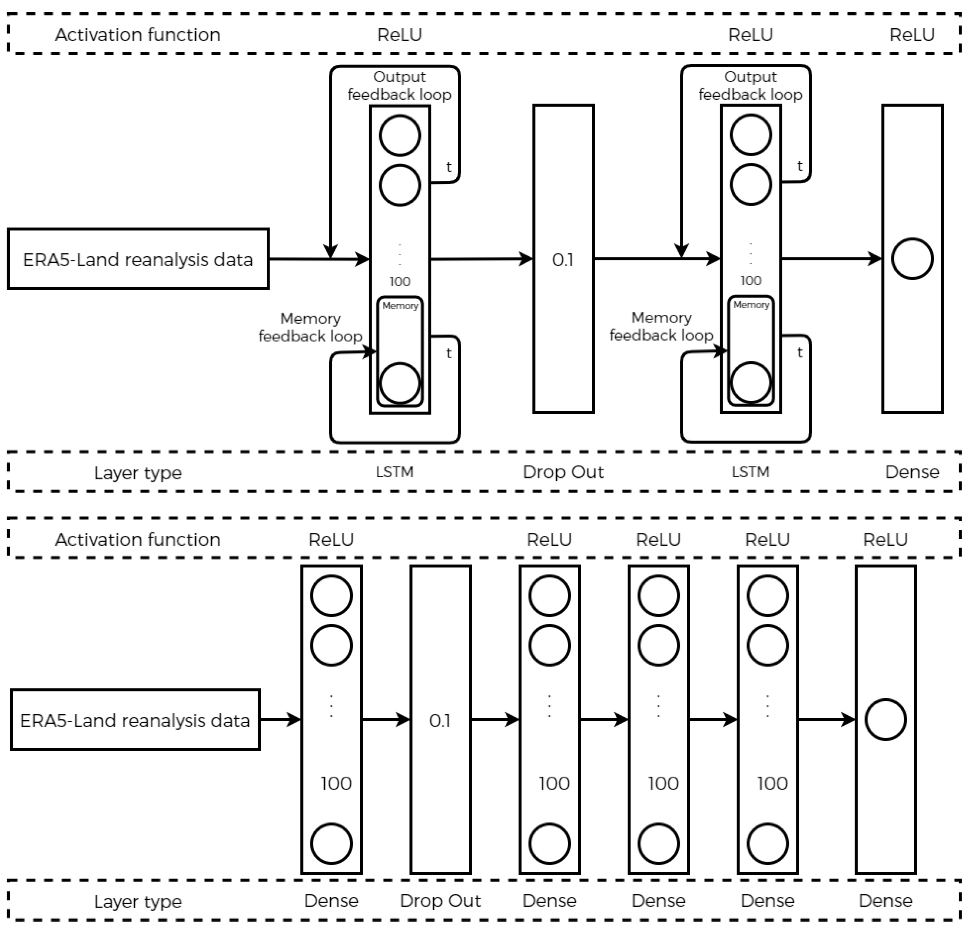
- c. Long Short-Term Memory (LSTM):
- d. Data normalization
- Min–max standardization: Min–max scales the feature values between [0, 1], with 0 being the feature’s minimum value and 1 being its maximum value, while maintaining the original distribution (Equation (10)).
- Decimal scaling: This form of scaling is used where values of different decimal ranges are present. For example, two features with different bounds can be brought to a similar scale using decimal scaling (Equation (11))
- Z-score: This transformation scales the value toward a normal distribution with a zero mean and unit variance using the z-score formula (Equation (12)).such that is the mean and is the standard deviation of the features’ distribution. This method is very efficient for datasets with a Gaussian distribution.
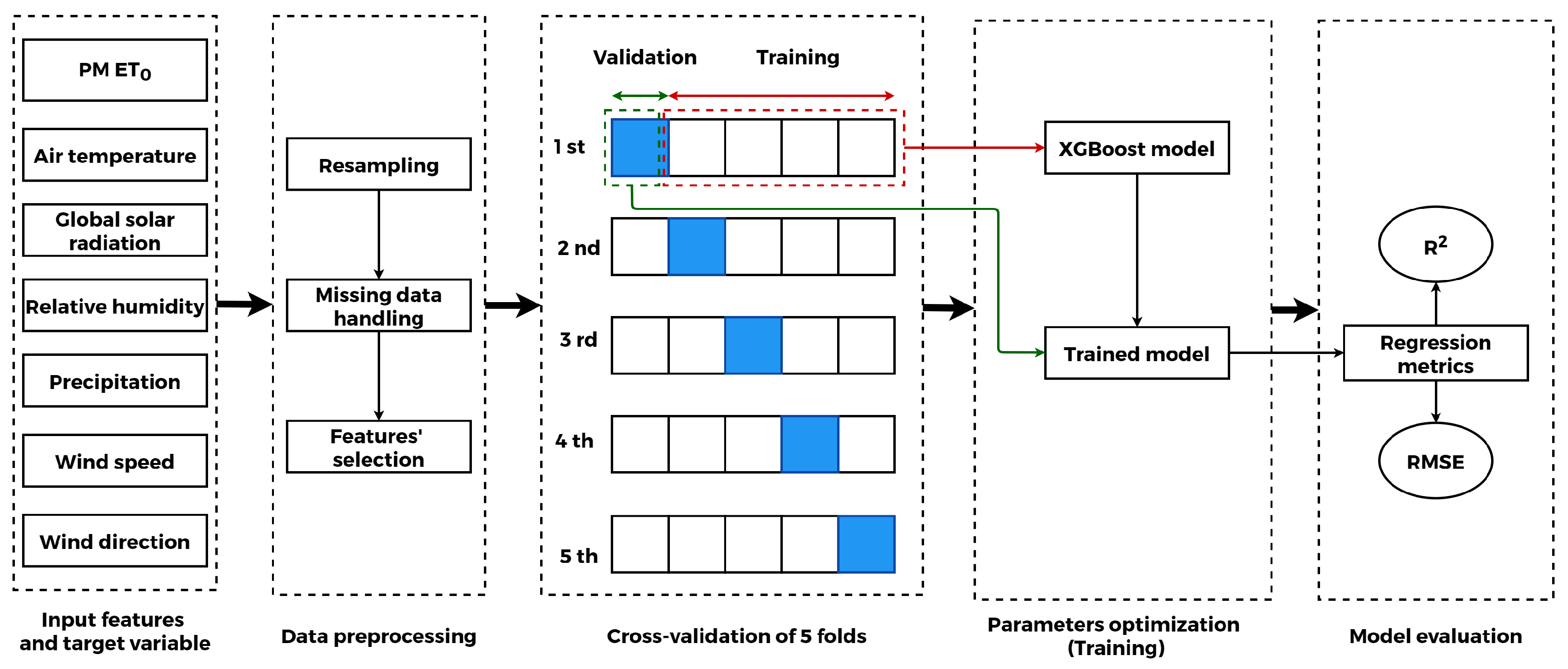
- e. Dataset splitting
- f. Evaluation Metrics
- Training time: The time it takes for the model to complete 20 epochs.
- R2 score or R2: The coefficient of determination informs about how well the unknown samples will be predicted by our model. It ranges between 0 and 1, but it can be negative as well (Equation (13)).
- The Pearson correlation coefficient (R): It measures the linear relationship between two normal distributed variables (Equation (14)).
- Root Mean Squared Error (RMSE): The average of the squares of the errors between real and predicted values by the model (Equation (15)).
- Mean Absolute Error (MAE): This is the average of absolute errors between real and predicted values (Equation (16)).
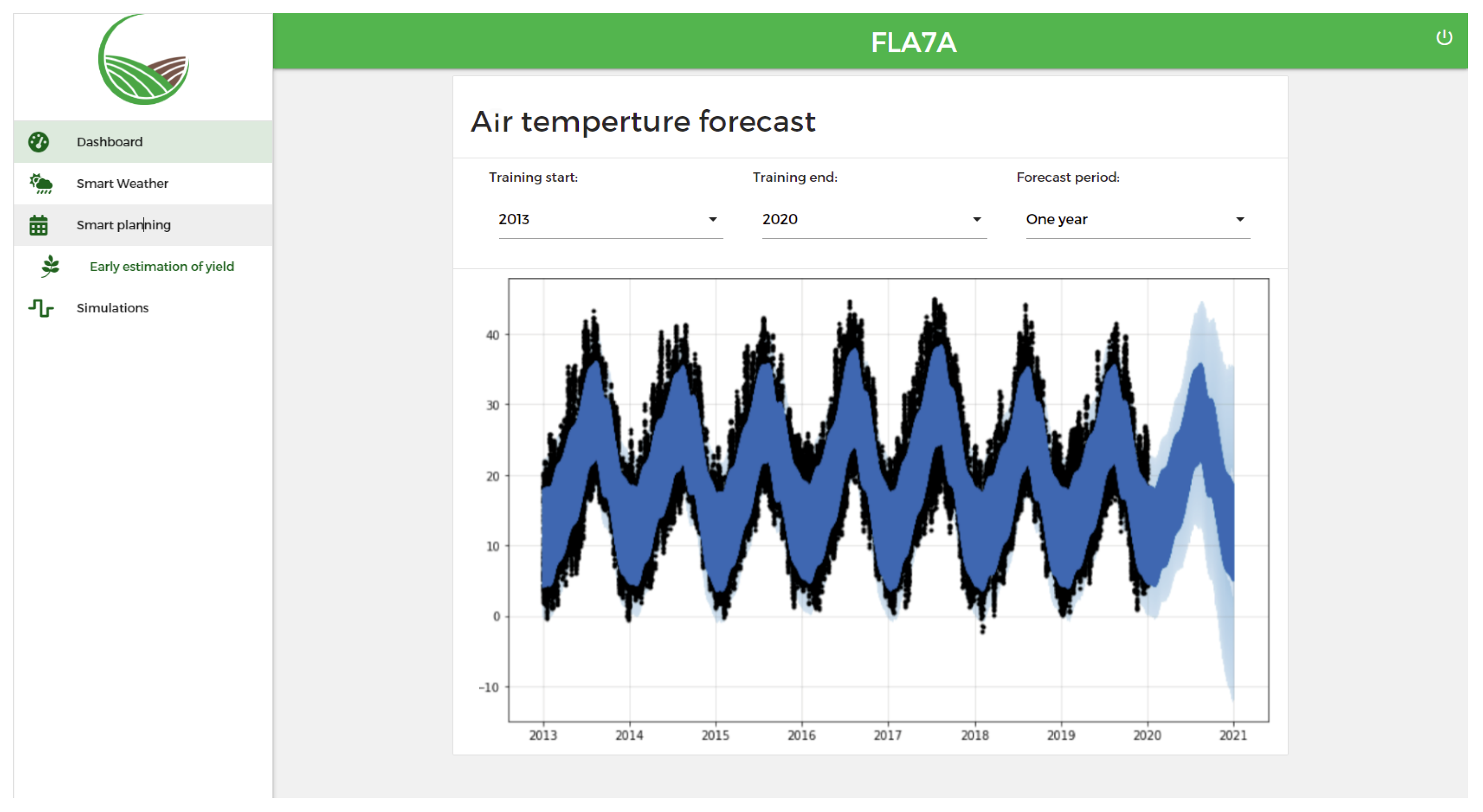
4.4.2. Forecasting Service
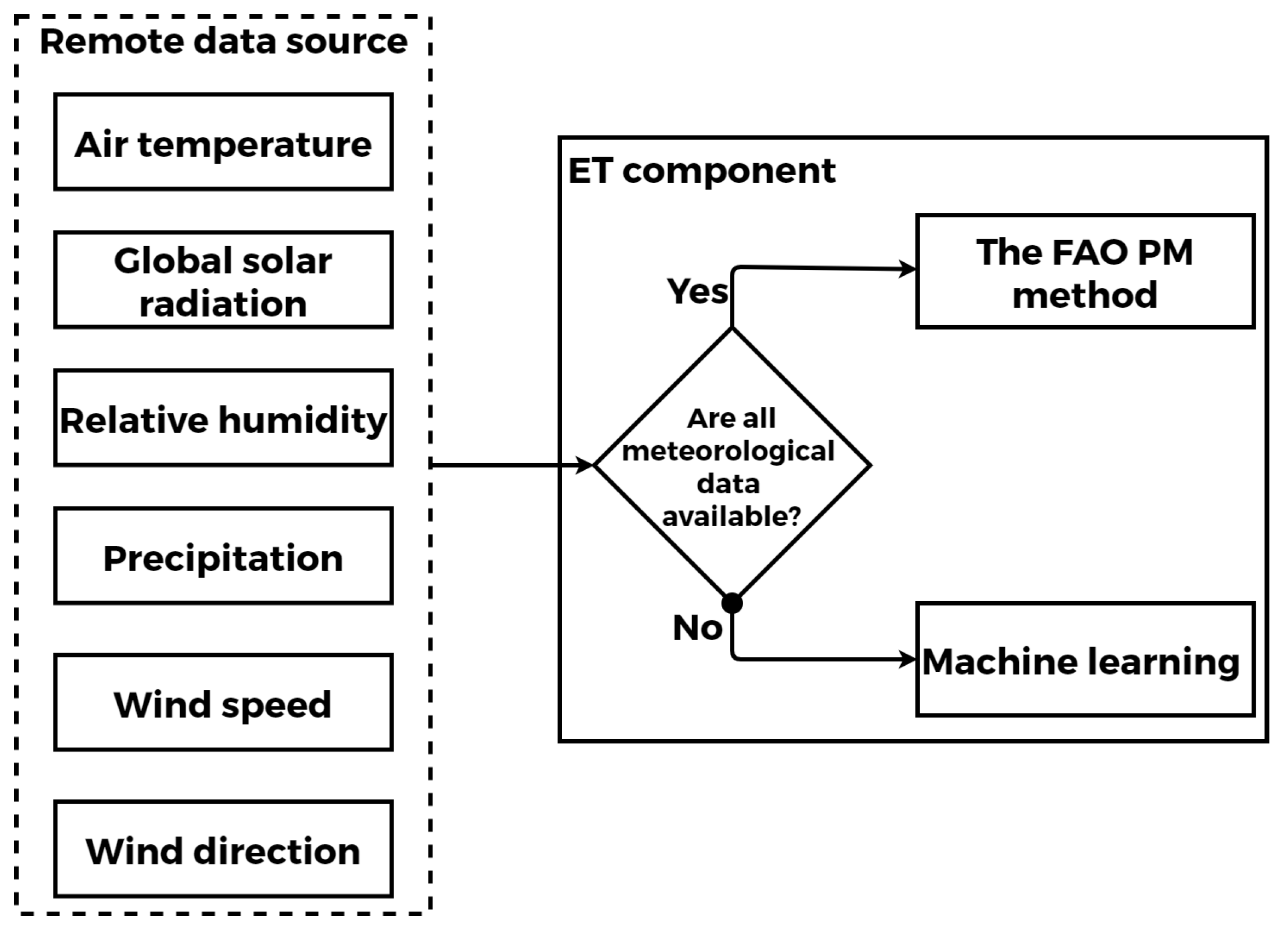
4.4.3. Climatic Parameters Calculation and Estimation Service
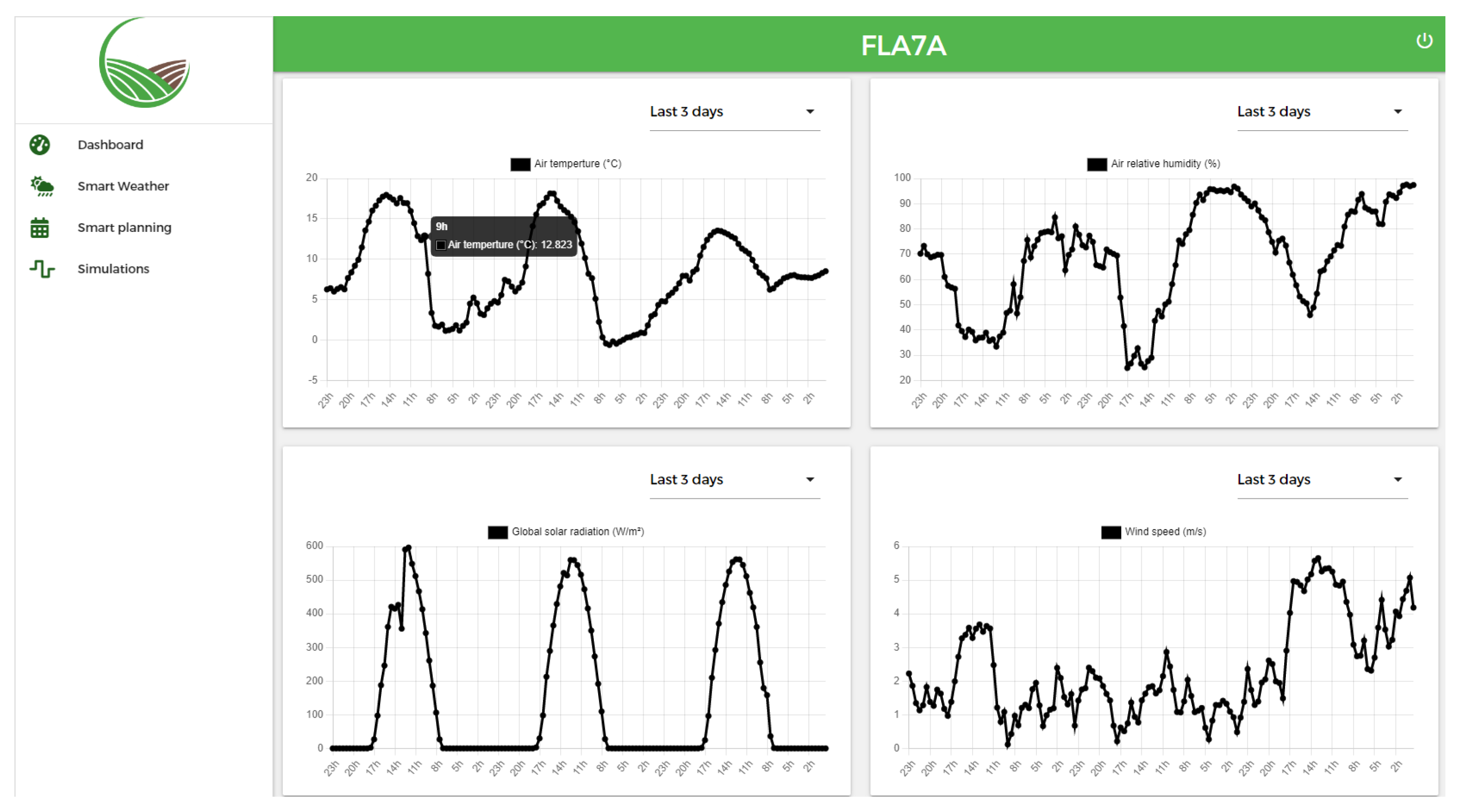
4.4.4. Weather Data Analysis and Visualization Service
4.4.5. Custom Early Warning Alerts Service
5. Results and Discussions
5.1. Time Series Data Imputation
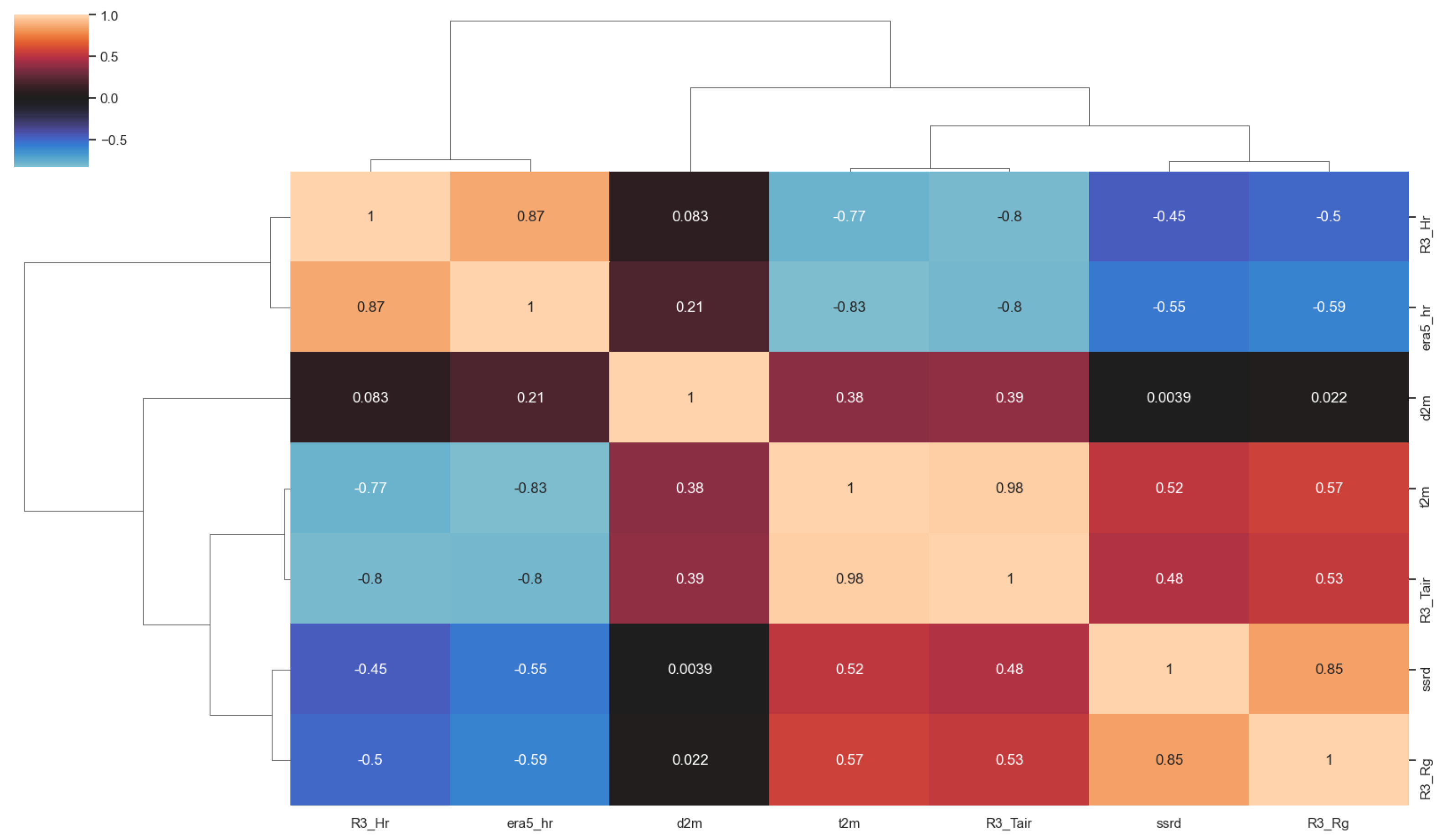
5.2. Climatic Parameters Calculation and Estimation
5.3. Prototype of the System
6. Conclusions
Author Contributions
Funding
Data Availability Statement
Acknowledgments
Conflicts of Interest
References
- Wade, M.; Hoelle, J.; Patnaik, R. Impact of Industrialization on Environment and Sustainable Solutions—Reflections from a South Indian Region. IOP Conf. Ser. Earth Environ. Sci. 2018, 120, 012016. [Google Scholar] [CrossRef]
- Bongaarts, J. Human population growth and the demographic transition. Philos. Trans. R. Soc. B Biol. Sci. 2009, 364, 2985. [Google Scholar] [CrossRef] [PubMed] [Green Version]
- Doungmanee, P. The nexus of agricultural water use and economic development level. Kasetsart J. Soc. Sci. 2016, 37, 38–45. [Google Scholar] [CrossRef] [Green Version]
- Frisvold, G.; Sanchez, C.; Gollehon, N.; Megdal, S.B.; Brown, P. Evaluating Gravity-Flow Irrigation with Lessons from Yuma, Arizona, USA. Sustainability 2018, 10, 1548. [Google Scholar] [CrossRef] [Green Version]
- Belaqziz, S.; Mangiarotti, S.; Le Page, M.; Khabba, S.; Er-Raki, S.; Agouti, T.; Drapeau, L.; Kharrou, M.H.; El Adnani, M.; Jarlan, L. Irrigation scheduling of a classical gravity network based on the Covariance Matrix Adaptation—Evolutionary Strategy algorithm. Comput. Electron. Agric. 2014, 102, 64–72. [Google Scholar] [CrossRef] [Green Version]
- Nafchi, R.A. Evaluation of the Efficiency of the Micro-irrigation Systems in Gardens of Chaharmahal and Bakhtiari Province of Iran. Int. J. Agric. Econ. 2021, 6, 106–110. [Google Scholar] [CrossRef]
- Norasma, C.Y.N.; Fadzilah, M.A.; Roslin, N.A.; Zanariah, Z.W.N.; Tarmidi, Z.; Candra, F.S. Unmanned Aerial Vehicle Applications In Agriculture. IOP Conf. Ser. Mater. Sci. Eng. 2019, 506, 012063. [Google Scholar] [CrossRef]
- Hersbach, H.; Bell, B.; Berrisford, P.; Hirahara, S.; Horányi, A.; Muñoz-Sabater, J.; Nicolas, J.; Peubey, C.; Radu, R.; Schepers, D.; et al. The ERA5 global reanalysis. Q. J. R. Meteorol. Soc. 2020, 146, 1999–2049. [Google Scholar] [CrossRef]
- Rienecker, M.M.; Suarez, M.J.; Gelaro, R.; Todling, R.; Bacmeister, J.; Liu, E.; Bosilovich, M.G.; Schubert, S.D.; Takacs, L.; Kim, G.K.; et al. MERRA: NASA’s Modern-Era Retrospective Analysis for Research and Applications. J. Clim. 2011, 24, 3624–3648. [Google Scholar] [CrossRef]
- Kobayashi, S.; Ota, Y.; Harada, Y.; Ebita, A.; Moriya, M.; Onoda, H.; Onogi, K.; Kamahori, H.; Kobayashi, C.; Endo, H.; et al. The JRA-55 Reanalysis: General Specifications and Basic Characteristics. J. Meteorol. Soc. Jpn. Ser. II 2015, 93, 5–48. [Google Scholar] [CrossRef]
- Kanamitsu, M.; Ebisuzaki, W.; Woollen, J.; Yang, S.K.; Hnilo, J.J.; Fiorino, M.; Potter, G.L. NCEP–DOE AMIP-II Reanalysis (R-2). Bull. Am. Meteorol. Soc. 2002, 83, 1631–1644. [Google Scholar] [CrossRef] [Green Version]
- Majumdar, P.; Mitra, S. IoT and Machine Learning-Based Approaches for Real Time Environment Parameters Monitoring in Agriculture: An Empirical Review. Agric. Inform. 2021, 5, 89–115. [Google Scholar] [CrossRef]
- Kumar, S.; Ansari, M.A.; Pandey, S.; Tripathi, P.; Singh, M. Weather Monitoring System Using Smart Sensors Based on IoT. Lect. Notes Netw. Syst. 2020, 106, 351–363. [Google Scholar] [CrossRef]
- Kodali, R.K.; Mandal, S. IoT Based Weather Station. In Proceedings of the 2016 International Conference on Control Instrumentation Communication and Computational Technologies, ICCICCT 2016, Kumaracoil, India, 16–17 December 2016; pp. 680–683. [Google Scholar] [CrossRef]
- Mittal, Y.; Mittal, A.; Bhateja, D.; Parmaar, K.; Mittal, V.K. Correlation among Environmental Parameters Using an Online Smart Weather Station System. In Proceedings of the 12th IEEE International Conference Electronics, Energy, Environment, Communication, Computer, Control: (E3-C3), INDICON 2015, Delhi, India, 17–20 December 2015. [Google Scholar] [CrossRef]
- Djordjević, M.; Jovičić, B.; Marković, S.; Paunović, V.; Danković, D. A smart data logger system based on sensor and Internet of Things technology as part of the smart faculty. J. Ambient Intell. Smart Environ. 2020, 12, 359–373. [Google Scholar] [CrossRef]
- Amin, F.; Abbasi, R.; Mateen, A.; Ali Abid, M.; Khan, S. A Step toward Next-Generation Advancements in the Internet of Things Technologies. Sensors 2022, 22, 8072. [Google Scholar] [CrossRef]
- Kamilaris, A.; Kartakoullis, A.; Prenafeta-Boldú, F.X. A review on the practice of big data analysis in agriculture. Comput. Electron. Agric. 2017, 143, 23–37. [Google Scholar] [CrossRef]
- Muangprathub, J.; Boonnam, N.; Kajornkasirat, S.; Lekbangpong, N.; Wanichsombat, A.; Nillaor, P. IoT and agriculture data analysis for smart farm. Comput. Electron. Agric. 2019, 156, 467–474. [Google Scholar] [CrossRef]
- Math, R.K.M.; Dharwadkar, N.V. IoT Based low-cost weather station and monitoring system for precision agriculture in India. In Proceedings of the 2nd International Conference on I-SMAC (IoT in Social, Mobile, Analytics and Cloud), Palladam, India, 30–31 August 2018; pp. 81–86. [Google Scholar] [CrossRef]
- Djordjevic, M.; Dankovic, D. A Smart Weather Station Based on Sensor Technology. Facta Univ. Ser. Electron. Energetics 2019, 32, 195–210. [Google Scholar] [CrossRef] [Green Version]
- Roukh, A.; Fote, F.N.; Mahmoudi, S.A.; Mahmoudi, S. WALLeSMART: Cloud Platform for Smart Farming. In Proceedings of the 32nd International Conference on Scientific and Statistical Database Management, Vienna, Austria, 7–9 July 2020. [Google Scholar] [CrossRef]
- Er-Raki, S.; Chehbouni, A.; Duchemin, B. Combining Satellite Remote Sensing Data with the FAO-56 Dual Approach for Water Use Mapping In Irrigated Wheat Fields of a Semi-Arid Region. Remote Sens. 2010, 2, 375–387. [Google Scholar] [CrossRef] [Green Version]
- Belaqziz, S.; Khabba, S.; Kharrou, M.H.; Bouras, E.H.; Er-Raki, S.; Chehbouni, A. Optimizing the Sowing Date to Improve Water Management and Wheat Yield in a Large Irrigation Scheme, through a Remote Sensing and an Evolution Strategy-Based Approach. Remote Sens. 2021, 13, 3789. [Google Scholar] [CrossRef]
- Er-Raki, S.; Chehbouni, A.; Guemouria, N.; Duchemin, B.; Ezzahar, J.; Hadria, R. Combining FAO-56 model and ground-based remote sensing to estimate water consumptions of wheat crops in a semi-arid region. Agric. Water Manag. 2007, 87, 41–54. [Google Scholar] [CrossRef] [Green Version]
- El Hachimi, C.E.; Belaqziz, S.; Khabba, S.; Chehbouni, A. Towards Precision Agriculture in Morocco: A Machine Learning Approach for Recommending Crops and Forecasting Weather. In Proceedings of the 2021 International Conference on Digital Age and Technological Advances for Sustainable Development, ICDATA 2021, Marrakech, Morocco, 29–30 June 2021; pp. 88–95. [Google Scholar] [CrossRef]
- Aouade, G.; Ezzahar, J.; Amenzou, N.; Er-Raki, S.; Benkaddour, A.; Khabba, S.; Jarlan, L. Combining stable isotopes, Eddy Covariance system and meteorological measurements for partitioning evapotranspiration, of winter wheat, into soil evaporation and plant transpiration in a semi-arid region. Agric. Water Manag. 2016, 177, 181–192. [Google Scholar] [CrossRef]
- Kharrou, M.H.; Simonneaux, V.; Er-Raki, S.; Le Page, M.; Khabba, S.; Chehbouni, A. Assessing Irrigation Water Use with Remote Sensing-Based Soil Water Balance at an Irrigation Scheme Level in a Semi-Arid Region of Morocco. Remote Sens. 2021, 13, 1133. [Google Scholar] [CrossRef]
- Oses, N.; Azpiroz, I.; Marchi, S.; Guidotti, D.; Quartulli, M.; Olaizola, I.G. Analysis of Copernicus’ ERA5 Climate Reanalysis Data as a Replacement for Weather Station Temperature Measurements in Machine Learning Models for Olive Phenology Phase Prediction. Sensors 2020, 20, 6381. [Google Scholar] [CrossRef] [PubMed]
- Zandler, H.; Senftl, T.; Vanselow, K.A. Reanalysis datasets outperform other gridded climate products in vegetation change analysis in peripheral conservation areas of Central Asia. Sci. Rep. 2020, 10, 22446. [Google Scholar] [CrossRef]
- Bui, M.T.; Lu, J.; Nie, L. Evaluation of the Climate Forecast System Reanalysis data for hydrological model in the Arctic watershed Målselv. J. Water Clim. Chang. 2021, 12, 3481–3504. [Google Scholar] [CrossRef]
- Muñoz-Sabater, J.; Dutra, E.; Agustí-Panareda, A.; Albergel, C.; Arduini, G.; Balsamo, G.; Boussetta, S.; Choulga, M.; Harrigan, S.; Hersbach, H.; et al. ERA5-Land: A state-of-the-art global reanalysis dataset for land applications. Earth Syst. Sci. Data 2021, 13, 4349–4383. [Google Scholar] [CrossRef]
- ERA5-Land Hourly Data from 1950 to Present. Available online: https://doi.org/10.24381/cds.e2161bac (accessed on 1 September 2022).
- Dee, D.P.; Uppala, S.M.; Simmons, A.J.; Berrisford, P.; Poli, P.; Kobayashi, S.; Andrae, U.; Balmaseda, M.A.; Balsamo, G.; Bauer, P.; et al. The ERA-Interim reanalysis: Configuration and performance of the data assimilation system. Q. J. R. Meteorol. Soc. 2011, 137, 553–597. [Google Scholar] [CrossRef]
- El Hachimi, C.; Belaqziz, S.; Khabba, S.; Chehbouni, A. Data Science Toolkit: An all-in-one python library to help researchers and practitioners in implementing data science-related algorithms with less effort. Softw. Impacts 2022, 1, 100240. [Google Scholar] [CrossRef]
- Taylor, S.J.; Letham, B. Forecasting at Scale. Am. Stat. 2018, 72, 37–45. [Google Scholar] [CrossRef]
- Chen, T.; Guestrin, C. XGBoost: A Scalable Tree Boosting System. In Proceedings of the ACM SIGKDD International Conference on Knowledge Discovery and Data Mining, San Francisco, CA, USA, 13–17 August 2016; pp. 785–794. [Google Scholar] [CrossRef] [Green Version]
- El Hachimi, C.; Belaqziz, S.; Khabba, S.; Chehbouni, A. Early Estimation of Daily Reference Evapotranspiration Using Machine Learning Techniques for Efficient Management of Irrigation Water. J. Phys. Conf. Ser. 2022, 2224, 012006. [Google Scholar] [CrossRef]
- Lawrence, M.G. The Relationship between Relative Humidity and the Dewpoint Temperature in Moist Air: A Simple Conversion and Applications. Bull. Am. Meteorol. Soc. 2005, 86, 225–234. [Google Scholar] [CrossRef]
- Parish, O.; Putnam, T.W. NASA Equations for the Determination of Humidity from Dewpoint and Psychrometric Data; NASA Dryden Flight Research Center: Hampton, VA, USA, 1977.
- Hochreiter, S. The Vanishing Gradient Problem During Learning Recurrent Neural Nets and Problem Solutions. Int. J. Uncertain. Fuzziness Knowl. Based Syst. 1998, 6, 107–116. [Google Scholar] [CrossRef] [Green Version]
- Bhanja, S.; Das, A. Impact of Data Normalization on Deep Neural Network for Time Series Forecasting. arXiv 2018. [Google Scholar] [CrossRef]
- Singh, D.; Singh, B. Investigating the impact of data normalization on classification performance. Appl. Soft Comput. 2020, 97, 105524. [Google Scholar] [CrossRef]
- Wirth, R.; Wirth, R. CRISP-DM: Towards a Standard Process Model for Data Mining. In Proceedings of the Fourth International Conference on the Practical Application of Knowledge Discovery And Data Mining, Denham, UK, 11–13 April 2000; pp. 29–39. [Google Scholar]
- Fayyad, U.; Piatetsky-Shapiro, G.; Smyth, P. The KDD process for extracting useful knowledge from volumes of data. Commun. ACM 1996, 39, 27–34. [Google Scholar] [CrossRef]
- Breuniq, M.M.; Kriegel, H.P.; Ng, R.T.; Sander, J. LOF: Identifying Density-Based Local Outliers. ACM SIGMOD Record 2000, 29, 93–104. [Google Scholar] [CrossRef]
- Carroll, A.B.; Wetherald, R.T. Application of Parallel Processing to Numerical Weather Prediction. J. ACM 1967, 14, 591–614. [Google Scholar] [CrossRef]
- Pal, M.; Deswal, S. M5 model tree based modelling of reference evapotranspiration. Hydrol. Process. 2009, 23, 1437–1443. [Google Scholar] [CrossRef]
- Yassin, M.A.; Alazba, A.A.; Mattar, M.A. Artificial neural networks versus gene expression programming for estimating reference evapotranspiration in arid climate. Agric. Water Manag. 2016, 163, 110–124. [Google Scholar] [CrossRef]
- Schultz, M.G.; Betancourt, C.; Gong, B.; Kleinert, F.; Langguth, M.; Leufen, L.H.; Mozaffari, A.; Stadtler, S. Can Deep Learning Beat Numerical Weather Prediction? Philos. Trans. R. Soc. A 2021, 379, 20200097. [Google Scholar] [CrossRef] [PubMed]
- Gessert, F.; Wingerath, W.; Friedrich, S.; Ritter, N. NoSQL database systems: A survey and decision guidance. Comput. Sci.—Res. Dev. 2016, 32, 353–365. [Google Scholar] [CrossRef]
- Shvachko, K.; Kuang, H.; Radia, S.; Chansler, R. The Hadoop Distributed File System. In Proceedings of the 2010 IEEE 26th Symposium on Mass Storage Systems and Technologies, MSST2010, Incline Village, NV, USA, 3–7 May 2010. [Google Scholar] [CrossRef]
- Zaharia, M.; Xin, R.S.; Wendell, P.; Das, T.; Armbrust, M.; Dave, A.; Meng, X.; Rosen, J.; Venkataraman, S.; Franklin, M.J.; et al. Apache spark: A unified engine for big data processing. Commun. ACM 2016, 59, 56–65. [Google Scholar] [CrossRef]
- Probst, P.; Bischl, B. Tunability: Importance of Hyperparameters of Machine Learning Algorithms. J. Mach. Learn. Res. 2019, 20, 1–32. [Google Scholar]
- Bergstra, J.; Ca, J.B.; Ca, Y.B. Random Search for Hyper-Parameter Optimization Yoshua Bengio. J. Mach. Learn. Res. 2012, 13, 281–305. [Google Scholar]
- Nouretdinov, I. Distributed Conformal Anomaly Detection. In Proceedings of the 2016 15th IEEE International Conference on Machine Learning and Applications (ICMLA), Anaheim, CA, USA, 18–20 December 2016; pp. 253–258. [Google Scholar] [CrossRef] [Green Version]
- Laxhammar, R.; Falkman, G. Online detection of anomalous sub-trajectories: A sliding window approach based on conformal anomaly detection and local outlier factor. IFIP Adv. Inf. Commun. Technol. 2012, 382, 192–202. [Google Scholar] [CrossRef]


| Variables | Description | Unit | Missing Values |
|---|---|---|---|
| R3_Dv | Wind direction | Degree | 2626 |
| R3_Hr | Relative air humidity | No unit | 2626 |
| R3_Rg | Global solar radiation | W m−2 | 5169 |
| R3_Tair | Air temperature | °C | 2631 |
| R3_Vv | Wind speed | m s−1 | 2626 |
| R3_P30m | Rainfall | mm | 2626 |
| Variables | Name | Description | Unit |
|---|---|---|---|
| Air temperature | Temperature of air at 2 m above the surface of land. | K | |
| Surface solar radiation downwards | Amount of solar radiation reaching the surface of Earth. It comprises both direct and diffuse solar radiation. | J m−2 | |
| Dewpoint temperature | The temperature to which the air, at 2 m above the surface of the Earth, would have to be cooled for saturation to occur. | K |
| Station Parameter | Correlation Based Potential Estimators | Ground-Truth-Based Potential Estimators |
|---|---|---|
| Air temperature () | , and | |
| Global solar radiation () | , and | |
| Air relative humidity () | and | , and |
| Hyperparameter or Layer | FFNN | LSTM |
|---|---|---|
| Epochs | 20 | 20 |
| Learning rate | 0.0001 | 0.0001 |
| Batch size | 64 | 64 |
| Layer 1 | 100 neurons | 100 LSTM unit |
| Layer 2 | 0.1 for dropout probability | 0.1 for dropout probability |
| Layer 3 | 100 neurons | 100 LSTM unit |
| Layer 4 | 100 neurons | 1 neuron |
| Layer 5 | 100 neurons | __ |
| Layer 6 | 1 neuron | __ |
| Metric/Model | FFNN | LSTM | ||||
|---|---|---|---|---|---|---|
| R3_Tair | R3_Rg | R3_Hr | R3_Tair | R3_Rg | R3_Hr | |
| Training time (s) | 68.371 | 34.943 | 60.639 | 138.193 | 65.574 | 178.503 |
| R2 | 0.957 | 0.838 | 0.768 | 0.957 | 0.839 | 0.812 |
| R | 0.978 | 0.916 | 0.877 | 0.978 | 0.916 | 0.901 |
| RMSE | 0.037 | 0.098 | 0.116 | 0.037 | 0.097 | 0.105 |
| MAE | 0.029 | 0.069 | 0.094 | 0.029 | 0.066 | 0.081 |
| Fold | All Variables | R3_Tair and R3_Rg | Only R3_Tair | |||
|---|---|---|---|---|---|---|
| R2 | RMSE | R2 | RMSE | R2 | RMSE | |
| 1 | 0.976094 | 0.080174 | 0.922928 | 0.258481 | 0.727668 | 0.913333 |
| 2 | 0.978442 | 0.092729 | 0.922629 | 0.332801 | 0.759759 | 1.033369 |
| 3 | 0.981453 | 0.066742 | 0.942489 | 0.206956 | 0.760640 | 0.861347 |
| 4 | 0.978672 | 0.085282 | 0.938638 | 0.245365 | 0.770725 | 0.916799 |
| 5 | 0.979803 | 0.081603 | 0.930292 | 0.281652 | 0.757509 | 0.979770 |
Disclaimer/Publisher’s Note: The statements, opinions and data contained in all publications are solely those of the individual author(s) and contributor(s) and not of MDPI and/or the editor(s). MDPI and/or the editor(s) disclaim responsibility for any injury to people or property resulting from any ideas, methods, instructions or products referred to in the content. |
© 2022 by the authors. Licensee MDPI, Basel, Switzerland. This article is an open access article distributed under the terms and conditions of the Creative Commons Attribution (CC BY) license (https://creativecommons.org/licenses/by/4.0/).
Share and Cite
Hachimi, C.E.; Belaqziz, S.; Khabba, S.; Sebbar, B.; Dhiba, D.; Chehbouni, A. Smart Weather Data Management Based on Artificial Intelligence and Big Data Analytics for Precision Agriculture. Agriculture 2023, 13, 95. https://doi.org/10.3390/agriculture13010095
Hachimi CE, Belaqziz S, Khabba S, Sebbar B, Dhiba D, Chehbouni A. Smart Weather Data Management Based on Artificial Intelligence and Big Data Analytics for Precision Agriculture. Agriculture. 2023; 13(1):95. https://doi.org/10.3390/agriculture13010095
Chicago/Turabian StyleHachimi, Chouaib El, Salwa Belaqziz, Saïd Khabba, Badreddine Sebbar, Driss Dhiba, and Abdelghani Chehbouni. 2023. "Smart Weather Data Management Based on Artificial Intelligence and Big Data Analytics for Precision Agriculture" Agriculture 13, no. 1: 95. https://doi.org/10.3390/agriculture13010095