Article

Simulation Analysis and Experiments for Blade-Soil-Straw Interaction under Deep Ploughing Based on the Discrete Element Method

1
Nanjing Institute of Agricultural Mechanization, Ministry of Agriculture and Rural Affairs, Nanjing 210014, China
2
Jiangsu Yanjiang Institute of Agricultural Sciences, Nantong 226012, China
*
Author to whom correspondence should be addressed.
Agriculture 2023, 13(1), 136; https://doi.org/10.3390/agriculture13010136
Submission received: 28 November 2022 / Revised: 22 December 2022 / Accepted: 27 December 2022 / Published: 5 January 2023
(This article belongs to the Special Issue 'Eyes', 'Brain', 'Feet' and 'Hands' of Efficient Harvesting Machinery)

Abstract

:
The desirable sowing period for winter wheat is very short in the rice-wheat rotation areas. There are also lots of straw left in harvested land. Deep rotary tillage can cover rice straw under the surface to increase soil organic matter. Clarifying the effect of the rotary tillage blade on the soil and straw, as well as analyzing the movement patterns and forces on the straw and soil, are essential to investigate the deep rotary tillage process in order to solve the problems of energy consumption and poor straw burial effect of deep tillage and deep burial machinery. In this study, we built the interaction model of rotary blade-soil-straw through the discrete element method to conduct simulation and identified the factors that affect the power consumption and operation quality of the rotary blade. The simulation process reflects the law of rotary blade-soil-straw interaction, and the accuracy of the simulation model has been verified by field trials. The simulation test results show that the optimized structural parameters of the rotary tillage blade were 210 mm, 45 mm, 37° and 115° (R, H, α and β) designed based on this theoretical model can cultivate to a depth of 200 mm. The operating parameters were 8π rad/s for rotational speed and 0. 56 m/s for forward speed, respectively; the simulated and field comparison tests were conducted under the optimal combination of parameters, and the power, soil breaking rate, and straw burial rate were 1.73 kW, 71.34%, and 18.89%, respectively; the numerical error rates of simulated and field test values were 6.36%, 5.42%, and 8.89%, respectively. The accuracy of the secondary model was verified. The simulation model had good accuracy at all factor levels. The model constructed in this study can provide a theoretical basis and technical reference for the interaction mechanism between rotary tillage and soil straw, the optimization of machine geometry, and the selection of operating parameters.

1. Introduction

Rotary tillers are widely used in the seed bed preparation segment of agricultural production [1]. The study demonstrated that a rotation tillage depth of 200 mm could fully mix the straw into the soil and significantly improve the sowing quality and wheat yield [2]. However, there are a significant number of challenges, such as insufficient tillage depth (less than 150 mm), unsatisfactory straw burying effect (low straw burying rate, insufficient straw burying depth), high power consumption, etc., in rice-wheat rotation areas. Moreover, long-term shallow rotational tillage results in a thinning and low-fertility soil tillage layer, which in turn leads to lower crop yields [3]. Simultaneously, inadequate straw mulching resulted in the distribution of straw in the upper part of the tillage layer, which allowed gaps between the top and bottom of the soil tillage layer, thus leading to segregation of the soil. It is easy to cause the next crop to fall dry and die, reducing the seeding rate in the cultivation area of two crops a year [4]. The concentration of a huge number of agricultural machines in the busy season, coupled with the increase in power consumption, is prone to air contamination [5,6], which is not in accordance with the concept of green development of agricultural machinery and decelerates the achievement of the carbon peaking and carbon neutral development goals.
To meet the above challenges and realize deep plowing, four solutions are applied in production practice as follows. (1) Increase the radius of the rotary blade. The test proved that the machine could achieve a tillage depth of 300 mm, but there are problems with the huge mechanism, heavy tillage load, and low reliability of the machine [7]. (2) Double-axis front shallow and behind deep rotary tillage. The machine sets two rows of knife rollers at the front and behind, the former for the first operation, the latter again, and finally, two operations to achieve deep tillage. In this solution, the soil accumulates in the gap between the front and rear blade axes of the machine, which interferes with the soil and prevents the rear blade axes from sinking into the ground. Moreover, the structure is complicated and heavy and consumes much energy [8,9]. (3) Submerged soil reversal rotary tillage. This solution is a tillage method in which the cutter shaft is reversed and submerged below the ground surface. This form of mechanism resulted in the transmission box and frame being difficult to enter the soil and congestion problems [10,11,12,13,14,15,16,17]. (4) Diagonal submerged soil reversal rotary tillage. This solution effectively solves the problem that the transmission box cannot enter the soil in the above two solutions. The blade roller is angled in the horizontal plane during the operation of the machine, and tillage is carried out obliquely, but there is a significant lateral force, which is not favorable for the operator to control the direction [18,19].
The structure of key components is unreasonable, and the equipment design lacks academic guidance. The above methods restrict the research progress of deep rotary tillage. The systematic study of rotary blade-soil-straw interaction in deep rotary tillage operation is insufficient, and the design of rotary tiller parameters and whole machine design lack theoretical support. This study synthesizes the research results in related fields of agricultural engineering and conducts research and discussion on the mechanism of rotary blade-soil-straw interaction in deep rotary tillage operation based on the discrete element method. The Discrete Element Method (DEM) is a numerical simulation method for basic research on solving discontinuous media problems [20]. It is different from the Finite Element Method (FEM) for solving continuous media problems. The basic principle of this method is to separate the research object into a set of rigid units. In order to make each unit conform to Newton’s second law, the motion equation of each unit is calculated by means of central difference, and the whole motion state and parameters of the research object are obtained. This method is favored by most researchers in the field of agricultural engineering. In this paper, the discrete element method is used to deal with the fact that the soil model is a discontinuous medium [21,22].
We have developed a discrete element model of rotary blade-soil-straw for issues such as soil breakage rate, straw displacement, and power consumption during observation of rotary tillage operation. After that, the prototype was tested according to the 3D model of the machine designed on the basis of this study, and field verification tests were done. Finally, the validity of the model was determined by comparing the results of field tests and simulation analysis. The structural arrangement of the remainder of this article is as follows: Part 2 describes the analysis of the relevant phenomena during the simulation test. Part 3 shows the relevant results. Part 4 presents the discussion of the test. Part 5 concludes and summarizes the whole article. In this study, a blade-soil-straw interaction model was established for rice-wheat rotation. The model can provide a theoretical basis and technical reference for the interaction mechanism between rotary tillage and soil straw, the optimization of machine geometry, and the selection of operating parameters.

2. Materials and Methods

2.1. Rotational Tillage Mechanism

2.1.1. Structure of Rotary Blades

The tractor is connected to the rotary tiller by a towing device and transmits power through a universal coupling. The schematic diagram of the rotary tiller is shown in Figure 1a. The rotary tiller moves forward with a tractor. The rotary tiller shaft rotates through the gearbox, following the tractor power output shaft to drive the rotary tiller. The scraper impacts and levels the scattered soil to achieve a flat cultivated land. In order to study the interaction rule of rotary tillage blade-soil-straw more intuitively, this paper first studies the operation mechanism of rotary tillage single blade-soil-straw and then optimizes the form and structure parameters of rotary tillage single blade.
The blade is the key working part of the rotary tiller. The shape and structural parameters of the blade badly affected the quality and power consumption of the rotary tiller. The blade in this paper is designed and researched based on a standard rotary tillage cutter according to the research objectives, as shown in Figure 1b. The remaining are implemented in accordance with GBT 5669-2017 Rotary Tillage Machine Blades and Holders. The main structural parameters are shown in Table 1.

2.1.2. Mechanisms of Rotary Blades

The values of forward velocity and linear velocity of the blade endpoint determine the normal progress of soil cutting operation. The blade endpoint presents a composite motion; therefore, arrangements of velocity parameters will have diverse trajectories.
Let Vd—the tangential velocity of the blade endpoint, m/s;
V d = R ω  
λ = V d V m
The blade velocity ratio λ and the motion trajectory are shown in Figure 2.
(1) When λ < 1, that is, the forward velocity Vm is greater than the blade linear velocity Vd, its motion trajectory is a short cycloid, the direction of the horizontal component of the linear velocity at any point on the cycloid is consistent with the forward direction, and it is hardly difficult to realize the operation of post throwing soil blocks.
(2) When λ = 1, that is, the two values are equal, its motion trajectory is a cycloid curve, The horizontal velocity at any point is zero, and the same as above cannot realize soil throwing.
(3) When λ > 1, that is, the forward velocity Vm is less than the blade’s linear velocity Vd, its motion trajectory is a complementary cycloid. The horizontal partial velocity direction of any point below the maximum cross chord is opposite to the forward direction, exact converse above, the soil block can be reprojected effectively at present.
Set point M is set as the blade cutting point; it will meet the normal working conditions of the rotary cultivator from the beginning of soil penetration to the end of soil throwing and leaving the ground; there are:
x = R cos α t + V m t
y = R sin cot t = R h
where R is the radius of gyration of a blade, with the unit of m, Vm is forward velocity, with the unit of m/s, ω is angular velocity, with the unit of rad/s, t is time, with the unit of s, h is tillage depth, with the unit of m.
To meet the condition of throwing soil backward, the horizontal partial velocity Vx of the absolute velocity at any point on the absolute motion track of the blade is less than 0, according to the above equation, let:
V x = d x d t = v m 2 ω sin ω t < 0
sin cot = R R h sin ω t = R R h
V m   < ( R h ) ω
The movement locus of the blade endpoint is shown in Figure 2b. As can be seen from the above equation: R increases, H increases, but the increased torque leads to increased power consumption, which leads to a decrease in speed and, therefore, productivity. Therefore, generally, R = 215, 245, 260 mm, and in this study, a range of 150 to 240 mm was chosen in order to explore whether a small radius could be used for rototilling under ground level.

2.2. The Discrete Element Model of Rotary Blade-Soil–Straw

2.2.1. Soil and Straw Model Parameters

The discrete element parameters consist of the intrinsic parameters (material density, Poisson’s ratio, shear modulus), material contact parameters (coefficient of restitution, coefficient of static friction, dynamic friction coefficient), and contact model parameters. The parameters employed in this article are taken from the reference [21]. The relevant parameters are shown in Table 2.
The increase in the number of particles in the software will lead to a decline in the geometric level of the simulation calculation speed [22]. In addition, too small particles will lead to an uncertain impact on the model under the micro force. Therefore, the size of the soil model is generally larger than the real soil particles in the simulation calculation. Without affecting the simulation test, the soil particle radius selected in this paper is 5 mm, 10 mm, 15 mm, and 30 mm, as shown in Figure 3.
In this paper, the rotary tillage blade mainly covers the straws scattered on the ground during operation and will not crush and cut the straws. For the purpose of improving the simulation efficiency, the straws established in this paper are also simplified to a certain extent. It is mainly composed of 10 particles with a radius of 5 mm. The center distance between adjacent particles is 5 mm. The total length of the straw model is 55 mm. The simulation model of straw is shown in Figure 4.

2.2.2. Contact Model Settings

Edem software 2018 integrates many options to apply to different material types of contact. We selected Hertz-Mindlin with Bonding along with the characteristics that the soil particles are difficult to reconnect after fracture in this paper. At the same time, the most commonly used contact theoretical model Hertz-Mindlin (no slip), is selected for ordinary contact calculation.
(a)
Hertz-Mindlin (no slip)
In this model, the normal force component model is based on the Hertzian contact theory. The tangential force component model is based on the work of Mindlin-Deresiewicz. Both normal and tangential forces have damping components, where the damping coefficient is related to the coefficient of restitution. The tangential friction force follows the Coulomb friction law, and the rolling friction adopts the research results of Sakaguchi. The relevant calculation principles are described in the literature [23,24,25,26,27,28].
The normal force Fn is expressed as follows:
F n = 4 3 E * R * δ n 3 2
1 E * = ( I v i 2 ) E i + ( 1 v j 2 ) E j
1 R * = 1 R i + 1 R j
where Fn is the normal force, with the unit of N, E* is equivalent to Young’s modulus, with the unit of Pa, R* is the equivalent radius, with the unit of m, δn is the amount of normal overlap, with the unit of m, vi,j is Poisson’s ratio, Ei,j is Particle Young’s modulus, with the unit of Pa, Ri,j is Particle radius, with the unit of m.
The normal damping force Fn d is expressed as follows:
F n d = 2 5 6 β S d m * v n r e l
β = ln e ln 2 e + π n 2
S n = 2 E * R * δ n
where Fn d is Normal damping force, with the unit of N, β is viscous damping coefficient, e is coefficient of restitution, Sn _is normal stiffness, with the unit of N/m, m* is equivalent mass, with the unit of g, mi,j is Particle mass, with the unit of g, v n   r e l is Normal relative velocity, with the unit of m/s.
The expression for the tangential force Ft is as follows:
F t = S t δ t
S t = 8 G * R * δ
where Ft is the normal force, N,St is tangential stiffness, with the unit of N/m, δt is tangential overlap, with the unit of m, G* is equivalent shear modulus, with the unit of Pa.
The tangential damping force Ftd is expressed as follows:
F t d = 2 5 6 β S t m * v t r e l
where Ftd is angential damping force, with the unit of N, St is tangential stiffness, with the unit of N/m, v t   r e l is Tangential relative velocity, with the unit of m/s.
The total tangential force is limited by the Coulomb friction force. When the tangential force reaches the Coulomb friction force, that is, Ft > μsFn, relative sliding occurs between the particles, where s is the static friction coefficient. To simplify the contact model, The model does not take into account the sliding friction of the contact model. The rolling friction is expressed in terms of the contact torque of the particle model, and the expression is as follows:
τ i = μ r F n R i ω i
where τi is torque, with the unit of N·m, μr is coefficient of rolling friction, Ri is the distance from the contact point to the centroid, with the unit of m, ωi—angular velocity of particles at the contact point, with the unit of r/min.
(b)
Hertz-Mindlin with Bonding
Hertz-Mindlin with Bonding contact model bonds particles together. Since this model includes Hertz-Mindlin (no slip), the default Hertz-Mindlin (no slip) contact model needs to be deleted from the software Creator Tree list when generating the bond.
Hertz-Mindlin with Bonding contact model uses finite-sized “bonding” bonds to bond particles. The bond can withstand the normal and tangential motion between the contacting particles to generate normal and tangential shear stress until the bond breaks at the critical maximum stress. The particles interact as rigid spheres, and no new bonds are generated, which is in line with the soil stress mechanical behavior characteristics of remaining loose after crushing [29,30,31].
In this model, the first generated particles interact with each other according to the Hertz-Mindlin contact model, and the connection starts after the set bond generation time point. After the particles are connected, the force and torque between the particles are both set to 0, according to the following Stepwise adjustment at each time step:
δ F n = v n S n A δ t
δ F t = v t S t A δ t
δ M n = ω n S t J δ t
δ M t = ω t S n J 2 δ t
A = π R B 2
J = 1 2 π R B 4
where Fn,t is normal and tangential force, with the unit of N, vn,t is normal and tangential velocity, with the unit of m/s, Sn,t is normal and tangential stiffness, with the unit of N/m, A is the cross-sectional area of bonding bond, with the unit of m2, δt is time step, with the unit of s, Mn,t is normal and tangential moments, with the unit of N·m, ωn,t is normal and tangential angular velocities, with the unit of r/min, J is the moment of inertia, with the unit of m4, RB is the bond-bond radius.
When the normal and tangential stresses exceed preset critical values, the bonded bonds will break, the particles will interact as rigid spheres, and no new bonds will be formed. Spawn bonds in this model can create cohesive forces when particles are generated, even if the particles are not in contact, so the contact radius should be set larger than the radius of the particle body.
Table 3 lists the parameters adopted in this study. In this article, we use Edem’s dynamic generation method to generate soil particle beds layer by layer, and the model is shown in Figure 5.
The particle contact model can quantify the interaction between discrete elements within a given contact range. Adding a contact model to the particle model is a key step in the test. Appropriate contact model to accelerate simulation test.

2.2.3. Initial Conditions for Simulation

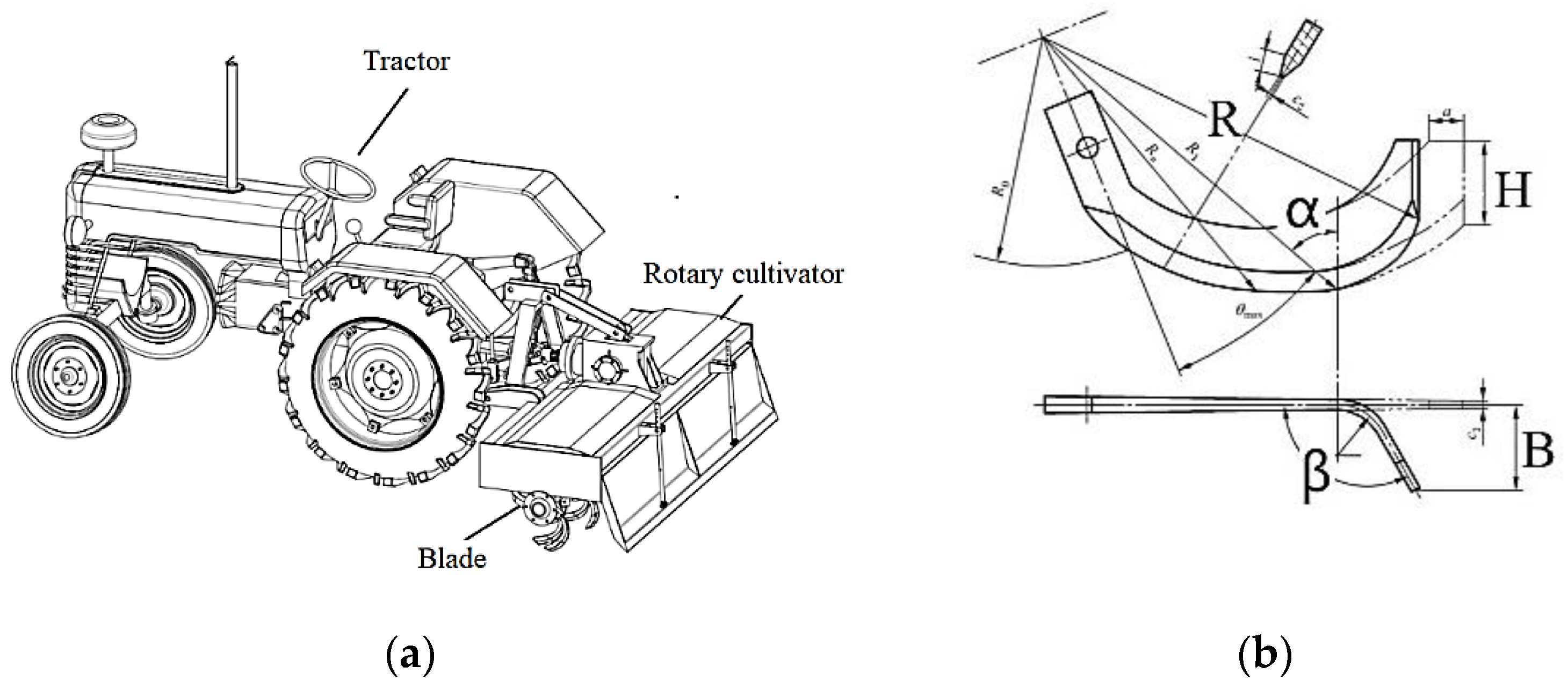
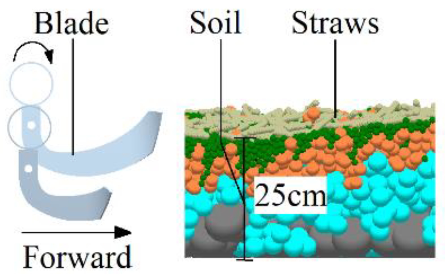
In this simulation test, in order to ensure that the tillage depth was equal to 200 mm, the rotation center was set to the corresponding position into the soil according to the radius of rotation of each blade, as shown in Figure 6.
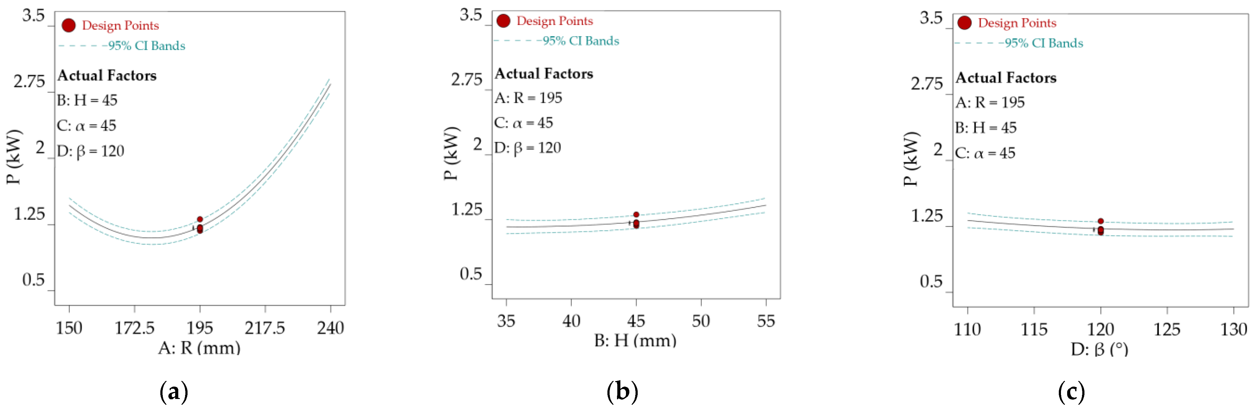
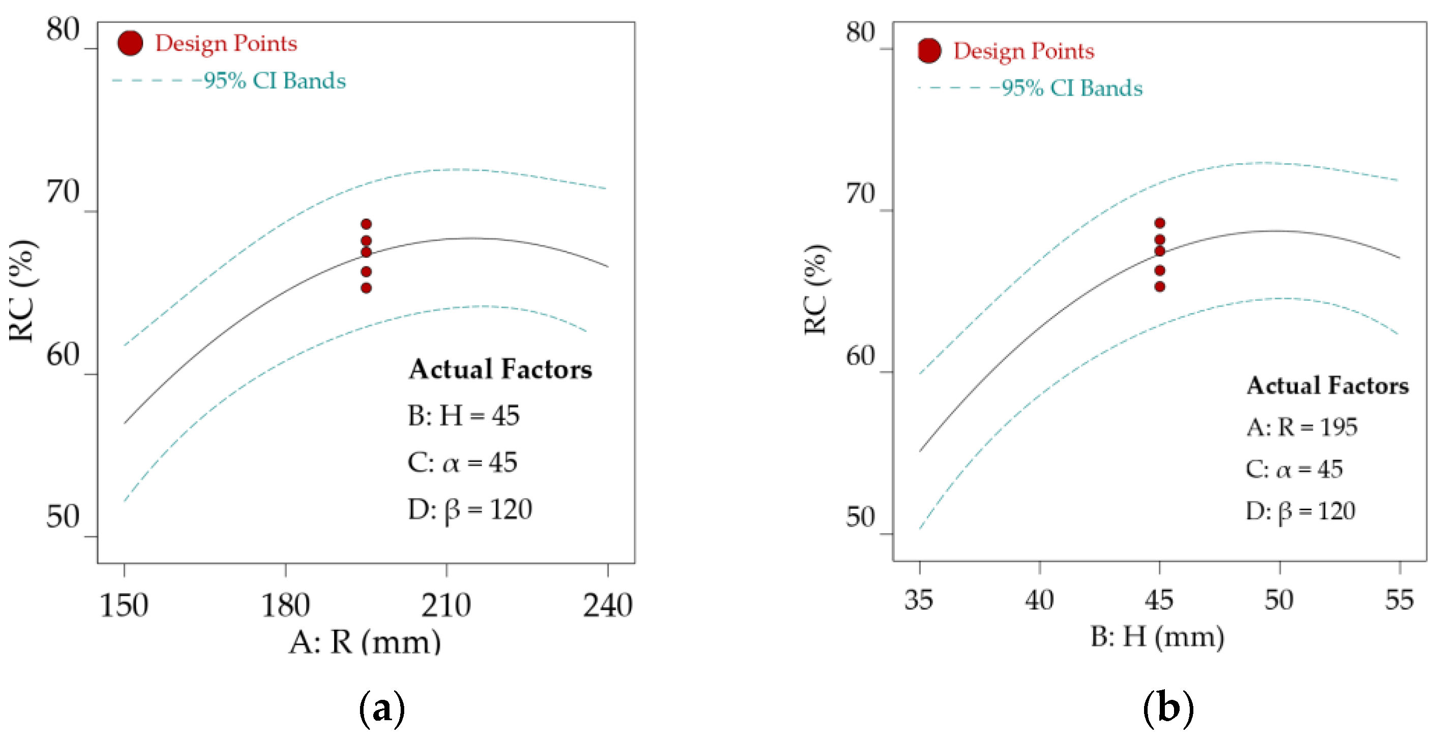
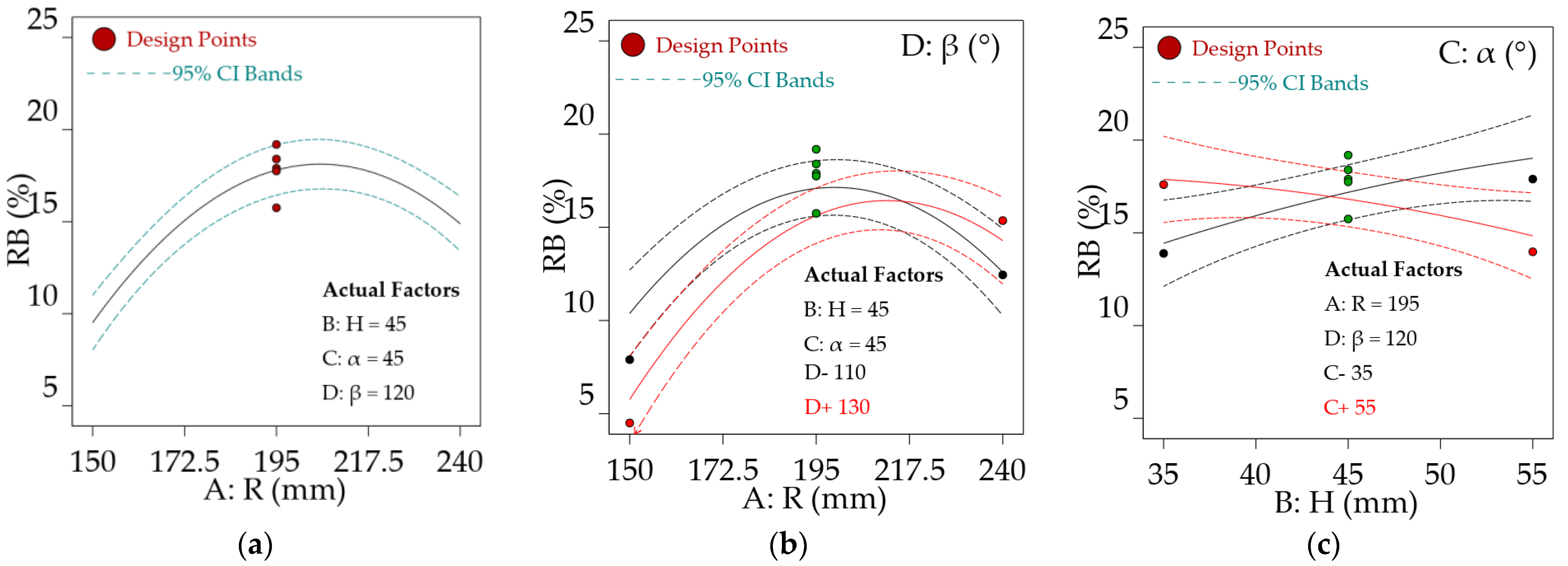
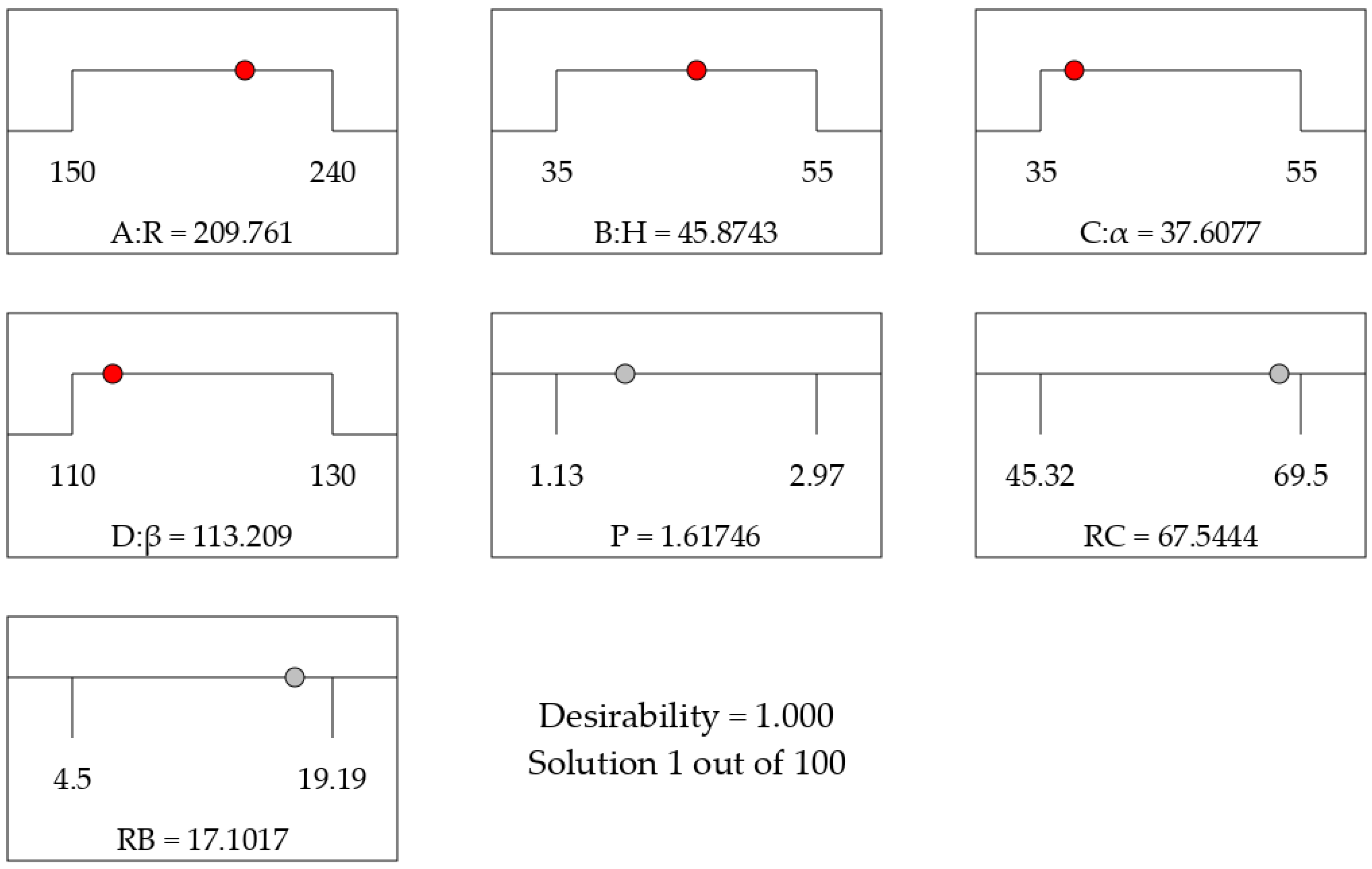
According to the research objectives of this article, combined with the existing re-search experience and actual working conditions, the main indicators were determined as the power (P), the rate of crushed soil (RC), and the rate of straw burial (RB). Figure 1b shows that the value of B is fixed when R and β are certain, so the factor B is removed. The initial conditions of the experiment are shown in Table 4, and the factor level design is shown in Table 5.
In this study, for convenience of calculation, the ratio of the number of bond-bond breaks per unit volume to the number of bond bonds at the beginning is used as the index of soil breakage. The sampling position is set 500 mm from the center of rotation after rotary tiller operation, and 1000 mm is set by grid-grid function after EDEM treatment.1000 mm × 500 mm × 250 mm grid solver calculates the bonding bond between particles as a problem to be solved.
The value of power (P) is selected from the data within 2 s of the operation stabilization stage. Each blade is tested three times, and the average value is obtained, which is directly exported after EDEM software post-processing.
The crushed soil rate (RC) is measured by the ratio of bond breakage between particles in the tillage area. In this study, for the convenience of calculation, the ratio of the number of soil bond breakage per unit volume to the number of bonded bonds at the initial time was used as the indicator of crushed soil rate. The sampling position was set at 500 mm from the center of rotation after the rotary tillage knife operation, and the grid solver of 1000 mm × 500 mm × 250 mm was set using the grid function of EDEM post-processing, and the particle-to-particle bond was calculated as the problem to be solved.
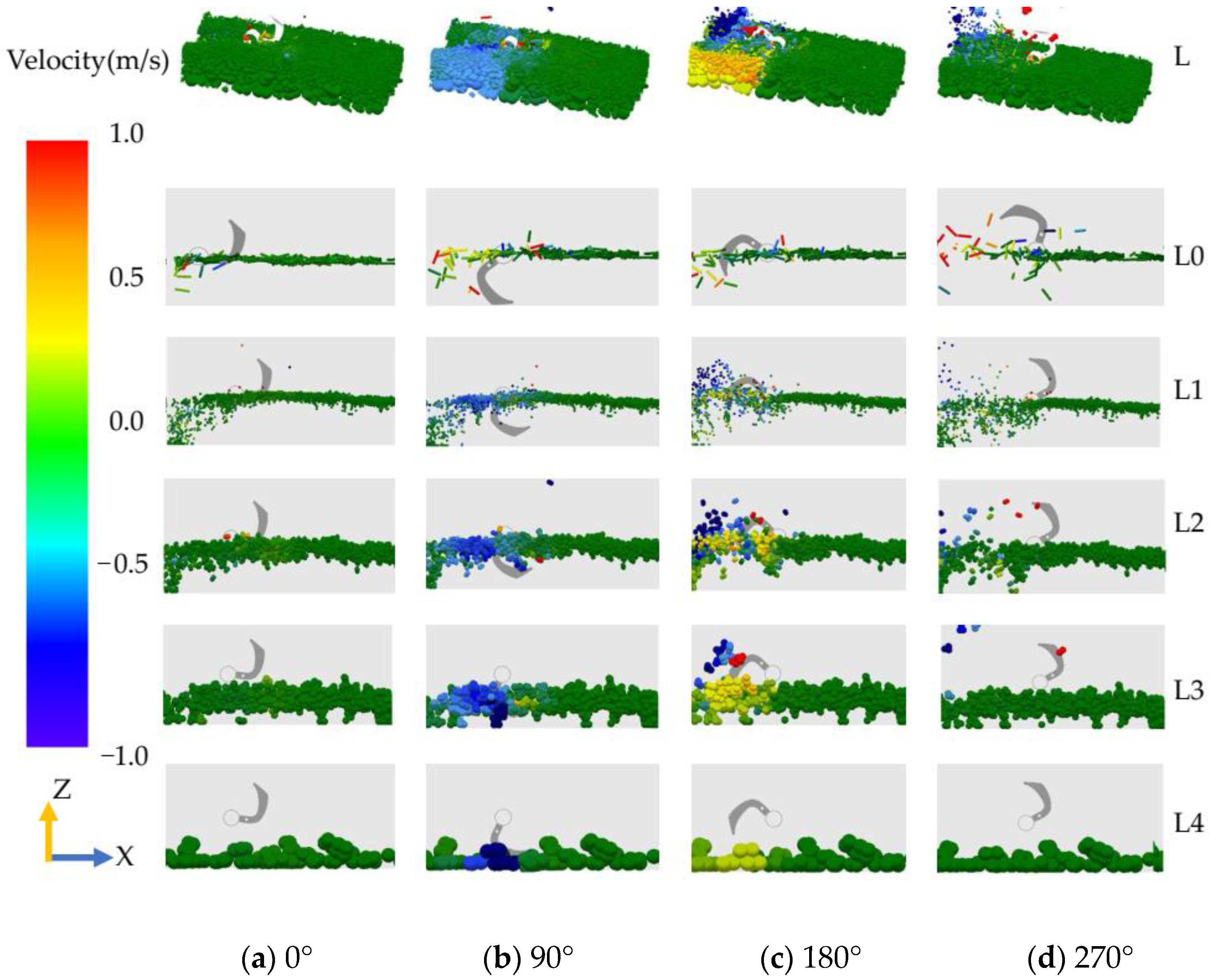
Straw burial rate (RB) is the percentage of straw residual mass on the ground post-tillage to the pre-tillage. In the post-processing of the EDEM software, L0 is the straw layer. The grid solver was divided into four layers (L1, L2, L3, L4) in the vertical direction, and the percentage of the total straw mass from L1 to L4 to the initial L0 mass was calculated as the straw burial rate.

2.3. Simulation

To better observe the movement of soil and straw in the simulation, we selected the velocity clouds from the simulation with different angles of blade rotation and placed them in Figure 7.
The velocity of the model is represented by the color-changing legend. The velocity ranges from green to red is 0–1 m/s, which means the velocity is the same as the forward direction. The velocity ranges from green to blue is 0–−1 m/s, which means the velocity is opposite to the forward direction. L refers to the whole tillage layer, L0 represents the straw, and L1–L4 represents the soil from 0–50 m, 50–100 mm, 100–150 mm, and 150–200 mm below the horizontal surface, respectively.
It can be seen from L: At 0° the rotary blade touches the soil, the soil and straw on the side edge are first disturbed by the force of the rotary blade, L1 soil, and L0 straw splash. The disturbed area has a definite initial velocity and appears yellow, representing a low value; At 90°, the rotary blade has fully entered the soil. The color of the soil and straw starts to change, which indicates that the number of particles gaining velocity starts to increase. At L, L0, and L1, it is clearly observed that the soil and straw near the rototiller knife are red and dark blue in color, with the majority of blue particles, which indicates that the velocity starts to increase and most of the soil acquires the initial velocity backwards. Concurrently, the color of the soil and straw on the other side was light blue, indicating that the latter was significantly more disturbed than the former, and the velocity was negative. At 180°, the rotary blade was about to break out of the soil. The soil near the front section of the rotary tiller is dark blue and blue, which means that the rotary tiller throws the soil in the lower part of the plow layer backwards and upwards. The color of the soil near the side edge of the rototiller is red, illustrating that the soil in this position moves forward with the rototiller. At this time, the color of the soil with greater disturbance on the left side changes to yellow, indicating that this part of the soil starts to move forward and gradually returns to its original state. The color of the thrown soil and straw particles changed after the rotary tillage knife came out of the soil, indicating that the soil and straw continued to move in the direction of the speed obtained when thrown and finally fell into the ground. The color of the disturbed area is dark green, demonstrating that the velocity returns to 0.
L0 and L1 received a significant disturbance. The soil close to the center is taken to L2 and L3 when the blade starts to cut the soil, and the soil far from the center is thrown upward and backward and finally falls into L2 and L4. L2 and L3 are disturbed similarly to L1 and L0. The soil far from the center is thrown out and finally falls into L1 and L3; For L4, the soil disturbance is minimal, but a small part of the soil far from the center is still affected by the force and acquires a certain initial velocity and flow.
The migration of the soil between L1 and L4 gives a side view of the mixing state of the tillage layer after rotary tillage. The more the layers migrate, the further they are from their original position and the better the mixing of the tillage layer. When the rototiller knife enters the soil again, it continues to disturb the soil after tillage, causing the straw to rebound and thus causing it to continue to migrate in the direction of the initial velocity. The soil is significantly displaced by the action of the rotary cutter, and the movement of the soil particles causes more significant displacement of the straw as the mechanical properties of the straw material are lower than those of the soil particles. The movement of the soil particles causes the straw to move more significantly due to the lower mechanical properties of the straw material than the soil particles. When the force is greater than the ultimate strength of the bond, the soil particles are separated and fractured, which means that the soil particles that were originally connected by the bond are separated and move to a different layer; as the tillage continues to advance, some of the particles will be separated by secondary cutting. During the tillage process, the soil is disturbed in different areas of the rototiller, with a clear range of disturbance away from the center. The surface of the tilled soil shows some undulations, mainly due to the fact that the tillage process has changed the surface form of the original soil, and there is a certain friction effect between the soil particles, which makes it difficult to recover the initial form.

2.4. Field Trials

In a comparison of the power consumption and operational effects of EDEM simulation and actual soil entry conditions, in field trials, the length of the experiment area is 200 m, and the width is 15 m. The experiment area belongs to the plain area with two crops a year, with an average annual precipitation of about 600 mm, and the soil texture is loam. The first crop of the experiment field is wheat, the vegetation coverage before tillage is 302.4 g/m2, the soil firmness of 0–250 mm thick is 2098.0 kPa, the absolute soil moisture content is 21.63%, the average volume mass is 1.67 g/cm3, and the temperature during the experiment is 28 °C. We connected the torque sensors and the farm machinery test box to the rotary tiller and the tractor and debugged them to ensure that the test system could complete the work normally, as shown in Figure 8.
The power (P) is measured by a torque sensor mounted between the tractor and the coupling.
The rate of soil crushed (RC) is determined by measuring a 200 mm × 200 mm × 200 mm full tilled layer of soil on ploughed land. The size of the sampled soil is divided into three classes according to their side lengths: 0–4 cm, 4–8 cm, and 8 cm or more, and the percentage of soil mass from 0–4 cm to the total mass is the rate of soil fragmentation, measured one point per stroke.
The straw burial rate (RB)was determined by separating and weighing the straw from the soil at 0–5 cm, 5–10 cm, 10–15 cm, 15–20 cm, and 20–25 cm. During the sampling process, samples were taken strictly in accordance with the sampling frame and the boundaries of the tillage layer. Straw beyond the boundaries was cut off with scissors, keeping only the straw within the boundaries of the sampling area, and finally, the weight of each layer was used for statistical analysis.
The rotary tiller was connected to the tractor through a three-point suspension, and the torque sensor was installed at the end of the power take-off shaft. The rotary tiller was connected to the tractor through a three-point suspension, and the torque sensor was installed at the end of the power take-off shaft. The rototiller is mounted in the middle of the blade shaft, and to facilitate the same experimental conditions as the simulation, the soil is treated as a monopoly with a height of 250 mm and a width of 200 mm to facilitate the entry of a 150 mm radius rototiller stick into the soil. The structure diagram is shown in Figure 9.

3. Results

3.1. Simulation Results

3.1.1. Results of Box-Behnken Design

Simulation tests were conducted according to the Box-Behnken design, with the power (P) and the rate of crushed soil (RC), and the rate of straw burial (RB) as the evaluation indexes, and the test results are shown in Table 6.

3.1.2. ANOVA for Quadratic Model

According to the data samples in Table 6, the quadratic model of power (P), rate of crushed soil (RC), and straw burial rate (RB) was calculated by Design-Expert 12.0 software:
  • Power (P)
According to the ANOVA results in Table 7, the Model F-value of 135.01 implies the model is significant. There is only a 0.01% chance that an F-value this large could occur due to noise. p-values less than 0.0500 indicate model terms are significant. In this case, A, B, D, A2, B2 are significant model terms. Values greater than 0.1000 indicate the model terms are not significant. Removing the insignificant term, the regression equation of the power consumption model in this study.
P = 1.22 + 0.6875 A + 0.1242 B 0.0492 D + 0.9322 A 2 + 0.0697 B 2
The ANOVA results showed that the interaction of the factors in this model was not significant, and only the radius (R), the end cutter height (H), and the bending angle (β) were significant among the factors. It can be found from Figure 10a that when H = 45, α = 45, β = 120, the power consumption value is the lowest when R is 180, which is 1.12 kW, and as the radius R gradually increases, the power consumption increases significantly, and the analysis of the reason is due to the increase of torque, which leads to the increase of power consumption; when the radius R is lower than 180 and starts to decrease, the reason for the increase of power consumption is that the center of the blade sinks too deep into the tillage layer, which causes the blade to repeatedly Cutting soil, unable to throw out the soil fully, causing an increase in power consumption. Figure 8b,c show that the power consumption decreases with the increase of H and increases with the decrease of β, respectively.
  • Rate of crushed soil (RC)
According to the ANOVA results in Table 8, the Model F-value of 4.00 implies the model is significant. There is only a 0.70% chance that an F-value this large could occur due to noise. p-values less than 0.0500 indicate model terms are significant. In this case, A, B, A2, B2 are significant model terms. Values greater than 0.1000 indicate the model terms are not significant. Removing the insignificant term, the regression equation of the rate of crushed soil model in this study.
R C = 67.31 + 4.82 A + 5.97 B 5.52 A 2 6.22 B 2
The ANOVA results showed that the interaction of the factors in this model was not significant. The radius (R) and the end cutter height (H) were significant among the factors. It can be found from Figure 11 that when H = 45, α = 45, β = 120, RC gradually increases with the increase of R and H. The curve stops growing at R = 195 and H = 45, respectively. The value of RC hovers around 68%. It indicates that the space for disturbing the soil at the same tillage depth under the action of a single blade is limited, and the scanning trajectory formed by its rotation is approximated.
  • Rate of straw burial (RB)
According to the ANOVA results in Table 9, the Model F-value of 11.95 implies the model is significant. There is only a 0.01% chance that an F-value this large could occur due to noise. p-values less than 0.0500 indicate model terms are significant. In this case, A, AD, BC, A2, D2 are significant model terms. Values greater than 0.1000 indicate the model terms are not significant. Removing the insignificant term, the regression equation of the rate of crushed soil model in this study is:
R B = 17.80 + 2.68 A + 1.58 A D 1.91 B C 5.60 A 2 1.44 D 2
The ANOVA results showed that the interaction of the factors in this model was significant. The R, Rβ, and Hα were significant among the factors. The trend of RB with R is shown in Figure 12a, which shows that the RB value increases and then decreases, with a maximum at R = 200 and a model prediction of 17.78%. This is due to the upper limit of the maximum straw burial capacity of a single blade role at the same tillage depth. Too small a blade radius causes the straw not to be fully tilled into the ground, and conversely, too large a radius causes the straw to be thrown farther by the blade, also preventing effective mulching. Figure 12b presents the interaction between R and β. It is clear that the effect of changing R on RB is similar to that shown in Figure 12a. Changing the value of β, when β is 110, the maximum value of RB is slightly less than that at 120. When β increases to 130, the extreme value of the variation curve decreases further, and the value of R is taken to 217.5. Figure 12c presents the interaction curve of H with α. It can be seen that the magnitude of α affects the trend of RB with H. This is because α affects the position of the bending line and, thus, the direction of the end line. α is 35, and RB decreases with increasing H. It can be seen that the larger H is at this angle, the more straw can be buried by a single blade. On the contrary, for α of 55, RB behaves in the opposite way to the above. The intersection points of the two are near H = 45.

3.2. Parameter Optimization and Comparison Test

The optimization function in Design-Expert 12.0 software was applied for the quadratic model in this study. The optimal parameters of the blade were obtained by solving the regression model with the conditions that the broken soil rate was taken as the minimum value of 65%, the minimum straw burial rate was 15%, and the power consumption was the lowest, as shown in Figure 13. The theoretical optimal parameters were obtained as the combination of radius (R) 209.761 mm, end face height (H) 45.8743 mm, pinch angle (α) 37.607°, and bending angle (β) 113.209°. In accordance with the actual fabrication process and practice, the values were taken as R = 210 mm, H = 45 mm, α = 37°, and β = 115°, etc.
A comparison test between the EDEM simulation and field was conducted under the optimal parameters to verify the reliability of the optimized parameters. Table 10 shows the results of this comparative test. The simulation test results showed that the power, soil breakage rate, and straw burial rate were 1.62 kW, 67.47%, and 17.21%, respectively; the field results showed that the power, soil breakage rate, and straw burial rate were 1.73 kW, 71.34% and 18.89%, respectively. The average error rates of the simulated and field test values were 6.36%, 5.42%, and 8.89%, respectively, which indicated that the model was a decent fit.

4. Discussion

(a)
Rotary blade radius R has the most obvious influence on the power consumption of single blade operation, while other indexes have no significant influence. If deep tillage is to be realized with small radius blades, the whole blade roll must be trapped in the inner part of the tillage layer in structural design, causing congestion and increasing power consumption; Conversely, using a blade with a large radius results in an increase in torque and a sharp increase in power consumption due to blade wear. The rotary tillage radius used in this paper is 210 mm, which can meet the purpose of 200 mm tillage depth and reduce power consumption at the same time. The reason for this is that a good mechanical structure and excellent operating performance make it stand out. Half of the rotary tiller rollers of this length fall into the tillage layer, which not only causes a sudden increase in power consumption caused by congestion but also achieves a good soil-cutting effect and reduces blade life loss;
(b)
The H had the most obvious effect on the straw cover rate. The reason is that they are close to the end of the blade and come into contact with the straw earlier, which has the most obvious impact on spraying and burying of straw. One of the objectives of this paper is to increase the straw cover rate and depth in order to better meet the agronomic requirements, reduce the straw residue on the surface of cultivated land, and bury it as far as possible to a deeper position in the tillage layer, so as to prevent the phenomenon of shelving and airing, and provide a good seeding bed for seeding. Considering comprehensively, 45 mm can meet the agronomic demand:
(c)
The α-influenced trend of each operation is different, so we can know by analyzing it. In the range of 35–55 with the increase of value, power consumption P first decreases and then increases and reaches the minimum value at 36. The reason for these changes is α. The size has different effects on the shape of the end of the blade. Too small a value will cause the forward cutting edge to turn outwards and the angle of penetration to become larger, resulting in flat cutting of the blade, which cannot effectively exert the soil cutting effect of the positive cutting edge of the blade. On the contrary, excessive value results in the form of a hook down on the positive cutting edge, which is easy to cause excavation of the positive cutting edge when cutting soil, and the soil carrying effect is improved, which is not conducive to the crushing of soil blocks;
(d)
Bending angle β affected trend of each index is basically the same; only the RB is greatly affected. Based on the research results, 115 degrees is selected as the optimal solution. The change of its value results in the change of bending degree of the forward cutting edge. The larger the value, the closer the blade approaches the straight blade, the higher the cutting performance, and the lower the throwing effect. The smaller the value, the opposite.
It is the first time, to our knowledge, that the effect of rototill blades on soil and straw after deep rototilling has been analyzed using tillage soil stratification to describe the effect of rototill blades on soil and straw in a rice-wheat rotation. This study reveals the interaction between the rototill blade and the soil and straw, a finding that will assist in the development of technologies for deep rototill straw burial operations. In addition, the design of deep rototill blades with improved blade-breaking energy and increased straw mulching rates could lead to the provision of good seedbeds.

5. Conclusions

In this study, a discrete meta-simulation model of rotary tillage knife-soil-straw interaction was developed. The interaction law of soil-touching components in deep tillage operation was explored, and the field experiment results also verified its usability. The optimized structural parameters of the rotary tillage blade were 210 mm-45 mm-37°-115° (R-H-α-β). The simulated and field comparison tests were conducted under the optimal combination of parameters, and the power, soil breaking rate, and straw burial rate were 1.73 kW, 71.34%, and 18.89%, respectively; the numerical error rates of simulated and field test values were 6.36%, 5.42%, and 8.89%, respectively. The accuracy of the secondary model was verified.
Note that the aim of the study was to investigate the interaction of the rotary single blade with the soil straw in deep rototilling operations, applicable to optimizing the structural parameters of the rotary blade, and our experiments found that the soil movement was more consistent with the simulation results, which confirmed the validity of the simulation model. Papers exploring the arrangement of the rototill knives and the operating parameters have been published in the literature and will be the focus of our future work. Deep rototill mulching of straw will also be a hot research issue in the tillage chain.

Author Contributions

Conceptualization, J.Z. (Jin Zhang) and C.W.; methodology, J.Z. (Jiping Zhu); software, J.Z. (Jin Zhang); validation, W.C., M.X. and D.Y.; formal analysis, J.Z. (Jin Zhang); investigation, M.X.; resources, W.C.; data curation, J.Z. (Jin Zhang); writing—original draft preparation, J.Z. (Jin Zhang); writing—review and editing, J.Z. (Jiping Zhu); visualization, J.Z. (Jiping Zhu); supervision, W.C.; project administration, M.X.; funding acquisition, J.Z. (Jiping Zhu). All authors have read and agreed to the published version of the manuscript.

Funding

The author thanks Jiping Zhu of Nanjing Institute of Agricultural Mechanization, Ministry of Agriculture and Rural Affairs for funding this work through the National Key Research and Development Program of China (2020YFD1000802), Jin Zhang of Jiangsu Yanjiang Institute of Agricultural Sciences for Science Fund for Young Scholars of Jiangsu Yanjiang Institute of Agricultural Sciences(YJ2022006), Liu Jian of Jiangsu Yanjiang Institute of Agricultural Sciences Jiangsu Province Science and Technology Project (BE2020388), Jiangsu Province Modern Agricultural Machinery Equipment and Technology Demonstration and Extension Project (NJ2020-04).

Institutional Review Board Statement

Not applicable.

Data Availability Statement

The data presented in this study are available within the article.

Acknowledgments

Thanks are due to Zhenggang Liu for assistance with the experiments and to Yurong Zhang for valuable discussion.

Conflicts of Interest

The authors declare no conflict of interest.

References

  1. Du, Z.H.; Chen, Y.Y.; Zhang, J.; Han, X.M.; Geng, A.J.; Zhang, Z.L. Development Status and Prospects of Rotary Farm Machinery in Domestic and Abroad. J. Chin. Agric. Mech. 2019, 40, 43–47. [Google Scholar]
  2. Zhou, J.H.; Wang, J.Y.; Meng, F.Y.; Tong, G.X.; Mei, L.; Liu, G.M.; Wang, Y.; Luo, J.; Xie, C.Y. Effects of Tillage Methods on Sowing Quality Yield and Benefit of Wheat. Crops 2022, 4, 199–204. [Google Scholar]
  3. Li, M.L.; Wang, W.D.; Han, K.; Wang, S.; Huang, Y.C.; Wang, Y.; Jia, B.Y. Influences of Rotary Tillage Depth, nitrogen Application Rate and Planting Density on Yield and Nitrogen Distribution and Utilization of Rice. Jiangsu Agric. Sci. 2021, 49, 55–61. [Google Scholar]
  4. Wang, L. Several Problems Needing Attention in Returning Corn Straw to the Field. Sci. Technol. Inf. 2011, 28, 28–356. [Google Scholar]
  5. Su, R.J. Environmental Pollution and Prevention of Agricultural Machinery. Hebei Agric. Mach. 2010, 06, 28–29. [Google Scholar]
  6. Yan, B.J. Brief Analysis on Environmental Pollution of Agricultural Mechanization and Countermeasure. Farm Mach. 2008, 14, 51–52. [Google Scholar]
  7. Xia, X.D.; Wu, C.Y.; Zhang, R.L.; Qiao, F.S. Development Prediction of Large and Efficient Rotary Tillage Machinery. Rural. Mech. 1999, 1, 75–78. [Google Scholar]
  8. Liang, X.Z.; Zhu, S.; He, Y.P. On the Design of Rotary Cultivation Parts for Biaxial Layered Soil Cultivators. Agric. Equip. Technol. 2020, 46, 42–44. [Google Scholar]
  9. Yang, Z.; Ge, X.Y.; Yang, D.H.; Lu, R.C.; Zhang, R.H. Research on Drive Improvement Design of Double-axle Rotary Tillage Duplex Operator. Agric. Equip. Technol. 2014, 40, 13–15. [Google Scholar]
  10. Liu, Y.Q.; Sang, Z.Z. Mathematical Model of Submerged Reverse Rotary Tiller and Parameters Optimization. Trans. Chin. Soc. Agric. Eng. 2000, 16, 88–91. [Google Scholar]
  11. Li, B.Q.; Chen, C.Y.; Liang, J. Proof of Theoretic Model for Latent Soil of Up-cut Rotary Cultivation and Optimization of Working Parameters. J. Jiangsu Univ. (Natl. Sci. Ed.) 2005, 26, 203–205. [Google Scholar]
  12. Li, B.; Chen, C. An Analysis on Collision of Throwing Soil with Cover of Latent Soil of Up-cut Rotary Cultivation. Trans. Chin. Soc. Agric. Mach. 1999, 06, 41–45. [Google Scholar]
  13. Chen, C.Y.; Gao, J.M. 3-d Scan and Data Treatment of Submerged Reverse-rotary Tiller. J. Agric. Mech. Res. 2007, 29–31, 56. [Google Scholar]
  14. Yan, J.C.; Li, H.C.; Hu, J.P. Study on Calculation of the Up-cut Rotary’s Throwing Soil Volume and Distribution. J. Agric. Mech. Res. 2014, 36, 29–33. [Google Scholar]
  15. Liu, Y.Q.; Sang, Z.Z. Effect of the Parameters of Submerged Reverse-rotary Blade on Energy Consumption. J. Jiangsu Univ. Sci. Technol. 2001, 04, 15–18. [Google Scholar]
  16. Jin, Y.; Gao, J.M. The Dynamic Balance of Cutter Roller Simulation Analysis of Oblique Rotary—Based on Pro/e and Adams. J. Agric. Mech. Res. 2013, 35, 160–162, 167. [Google Scholar]
  17. Kong, L.D.; Sang, Z.Z.; Wang, G.L. The Development of Three Dimensional Convexity of Oblique Rotary Tillage. Trans. Chin. Soc. Agric. Mach. 2000, 31, 28–31. [Google Scholar]
  18. Kong, L.D.; Sang, Z.Z.; Wang, G.L. Experimental Study on Oblique Rotary Tillage. Trans. Chin. Soc. Agric. Mach. 2000, 2, 31–34. [Google Scholar]
  19. Kong, L.D.; Sang, Z.Z. The Research of Oblique Rotary Tillage. J. Taiyuan Heavy Mach. Inst. 1999, 31, 310–313, 343. [Google Scholar]
  20. Zeng, Z.W.; Ma, X.; Cao, X.L.; Li, Z.H.; Wang, X.C. Critical Review of Applications of Discrete Element Method in Agricultural Engineering. Agric. Eng. 2021, 11, 29–34. [Google Scholar]
  21. Fang, H.M.; Ji, C.Y.; Farman, A.C.; Guo, J.; Zhang, Q.Y.; Chaudhry, A. Analysis of Soil Dynamic Behavior During Rotary Tillage Based on Distinct Element Method. Trans. Chin. Soc. Agric. Mach. 2016, 47, 22–28. [Google Scholar]
  22. Mustafa, U.; John, M.F.; Chris, S. 3D DEM tillage simulation: Validation of a hysteretic spring (plastic) contact model for a sweep tool operating in a cohesionless soil. Soil Tillage Res. 2014, 144, 220–227. [Google Scholar]
  23. Fang, H.M.; Ji, C.Y.; Zhang, Q.Y.; Guo, J. Force Analysis of Rotary Blade Based on Distinct Element Method. Trans. Chin. Soc. Agric. Eng. 2016, 32, 54–59. [Google Scholar]
  24. Sakaguchi, H. Plugging of the Flow of Granular Materials During the Discharge from a Silo. Int. J. Mod. Phys. B 1993, 7, 1949–1963. [Google Scholar] [CrossRef]
  25. Cundall, P.; Strack, O.A. Discrete Numerical Model for Granular Assemblies. Geotechnique 1979, 29, 47–65. [Google Scholar] [CrossRef]
  26. Hertz, H. On the Contact of Elastic Solids. J. Fur Die Reine Und Angew. Math. 1882, 92, 156–171. [Google Scholar] [CrossRef]
  27. Mindlin, R.D.; Deresiewicz, H. Elastic Spheres in Contact Under Varying Oblique Forces. J. Appl. Mech. 1953, 16, 327–344. [Google Scholar] [CrossRef]
  28. Mindlin, R.D. Compliance of Elastic Bodies in Contact. J. Appl. Mech. 1949, 16, 259–268. [Google Scholar] [CrossRef]
  29. Tsuji, Y. Lagrangian Numerical Simulation of Plug Flow of Cohesionless Particles in a Horizontal Pipe. Powder Technol. 1992, 71, 239–250. [Google Scholar] [CrossRef]
  30. Potyondy, D.; Cundall, P.A. Bonded-particle Model for Rock. Int. J. Rock Mech. Min. Sci. 2004, 41, 1329–1364. [Google Scholar] [CrossRef]
  31. Zhang, J.; Chen, W.; Tashi, N.; Zhu, J.P.; Ding, Y.; Yuan, D.; Yao, K.H.; Xia, M. Design and Analysis of Energy-saving Forward Deep rotary Tillage Machine. Agric. Mech. Asia 2021, 52, 4935–4949. [Google Scholar]
Figure 1. Standard rotary tiller structure.
Agriculture 13 00136 g001
Figure 2. Blade end point motion track.
Agriculture 13 00136 g002
Figure 3. Soil particles with different sizes.
Agriculture 13 00136 g003
Figure 4. Straw model.
Agriculture 13 00136 g004
Figure 5. The discrete element model.
Agriculture 13 00136 g005
Figure 6. Initial position of the rotary blade.
Agriculture 13 00136 g006
Figure 7. Velocity of soil and straw in different tillage layers during single blade operation.
Agriculture 13 00136 g007
Figure 8. Data acquisition hint.
Agriculture 13 00136 g008
Figure 9. Schematic diagram of field test component links.
Agriculture 13 00136 g009
Figure 10. Power consumption value at different factors.
Agriculture 13 00136 g010
Figure 11. Rate of crushed soil value at different factors.
Agriculture 13 00136 g011
Figure 12. Rate of straw burial value at different factors.
Agriculture 13 00136 g012
Figure 13. Parameter optimization of theoretical values.
Agriculture 13 00136 g013
Table 1. The main structural parameters.
SymbolNameNumerical Value
RRadius of gyration150~245 mm
BWorking breadth35~55 mm
HEnd cutter height35~55 mm
αIncluded angle35~55°
βBending angle110~130°
Table 2. Material physical properties parameters.
MaterialDensity (g/cm3)Poisson’s RatioShear Modulus (Pa)
Soil1.6680.381.0 × 106
Straw0.2270.401.0 × 106
65Mn7.8000.307.9 × 1010
Table 3. Contact parameters.
ContactsCoefficient of RestitutionCoefficient of Static FrictionDynamic Friction Coefficient
Soil-soil0.60.60.40
Soil-straw0.50.50.05
Soil-65Mn0.60.60.05
Straw-straw0.30.30.01
Straw-65Mn0.30.30.01
Table 4. Initial conditions.
Radius (mm)Center of Rotation (mm)Revs (rad/s)Velocity (m/s)
150−500.56
195−50.56
245450.56
Table 5. Factor levels.
LevelsR (mm)H (mm)α (°)β (°)
−11503535110
01954545120
12455555130
Table 6. Design and results of Box-Behnken Design.
StdRunFactorsResponses
A:R(mm)B:H(mm)C:α(°)D:β(°)P(kW)RC(%)RB(%)
12915035451201.4749.5009.60
22224035451202.8660.2814.09
31015055451201.5258.2011.50
42024055451202.9261.0814.56
5619545351101.2769.5017.60
61819545551101.3564.2918.09
71619545351301.2964.2915.34
81419545551301.1765.0913.98
91515045451101.5956.4007.90
10524045451102.9769.0912.45
11315045451301.5152.4004.50
121324045451302.7862.3015.36
13819535351201.1845.3213.89
14719555351201.5067.0917.90
15419535551201.1645.8017.60
16919555551201.5264.9013.98
172415045351201.5652.1009.30
182524045351202.9260.0914.09
192115045551201.4654.3008.90
202324045551202.9167.9013.35
211919535451101.2453.0917.39
222619555451101.5664.2015.39
232719535451301.1359.2013.50
24119555451301.5169.4017.36
251219545451201.2269.2318.40
261719545451201.3167.5019.19
27219545451201.1865.3015.75
282819545451201.268.2017.90
291119545451201.2166.3017.75
Table 7. ANOVA for Quadratic model of Power.
SourceSum of SquaresdfMean SquareF-Valuep-Value
Model11.79140.8422135.01<0.0001
A-R5.6715.67909.20<0.0001**
B-H0.185010.185029.66<0.0001**
C-α0.001910.00190.30060.5922
D-β0.029010.02904.650.0489*
AB0.000010.00000.00400.9504
AC0.002010.00200.32460.5779
AD0.003010.00300.48490.4976
BC0.000410.00040.06410.8038
BD0.000910.00090.14430.7098
CD0.010010.01001.600.2261
A25.6415.64903.50<0.0001**
B20.031510.03155.050.0413*
C20.007810.00781.250.2824
D20.012910.01292.070.1718
Residual0.0873140.0062
Lack of Fit0.0772100.00773.050.1468
Pure Error0.010140.0025
Cor Total11.8828
** indicates highly significant (p < 0.01), * indicates significant (p < 0.05), and p-values greater than 0.1000 indicate the model terms are not significant.
Table 8. ANOVA for Quadratic model of Rate of crushed soil.
SourceSum of SquaresdfMean SquareF-Valuep-Value
Model1175.901483.994.000.0070
A-R278.791278.7913.280.0027**
B-H428.171428.1720.390.0005**
C-α1.2611.260.06010.8100
D-β1.2611.260.06010.8100
AB15.60115.600.74310.4032
AC7.8717.870.37470.5503
AD1.9511.950.09270.7653
BC1.7811.780.08490.7751
BD0.207010.20700.00990.9223
CD9.0319.030.43010.5226
A2197.891197.899.420.0083**
B2251.031251.0311.960.0038**
C274.75174.753.560.0801**
D20.205110.20510.00980.9227
Residual293.961421.00
Lack of Fit284.391028.4411.880.0146
Pure Error9.5742.39
Cor Total1469.8628
** indicates highly significant (p < 0.01), and p-values greater than 0.1000 indicate the model terms are not significant.
Table 9. ANOVA for Quadratic model of Rate of straw burial.
SourceSum of SquaresdfMean SquareF-Valuep-Value
Model337.331424.1011.95<0.0001
A-R86.40186.4042.86<0.0001**
B-H1.7811.780.88230.3635
C-α0.410710.41070.20370.6586
D-β6.4216.423.190.0959
AB0.511210.51120.25360.6224
AC0.028910.02890.01430.9064
AD9.9519.954.940.0433*
BC14.55114.557.220.0177*
BD8.5818.584.260.0581
CD0.855610.85560.42440.5253
A2203.401203.40100.90<0.0001**
B21.3411.340.66560.4282
C24.1214.122.050.1746
D213.49113.496.690.0215*
Residual28.22142.02
Lack of Fit21.72102.171.330.4194
Pure Error6.5141.63
Cor Total365.5528
** indicates highly significant (p < 0.01), * indicates significant (p < 0.05), and p-values greater than 0.1000 indicate the model terms are not significant.
Table 10. Comparison of simulation and test results under optimal parameters.
ResponsesField TestSimulationError (%)
P (kW)1.731.626.36
RC (%)71.3467.475.42
RB (%)18.8917.218.89
Disclaimer/Publisher’s Note: The statements, opinions and data contained in all publications are solely those of the individual author(s) and contributor(s) and not of MDPI and/or the editor(s). MDPI and/or the editor(s) disclaim responsibility for any injury to people or property resulting from any ideas, methods, instructions or products referred to in the content.

