Causal Linkage among Agricultural Insurance, Air Pollution, and Agricultural Green Total Factor Productivity in United States: Pairwise Granger Causality Approach

Abstract

Agricultural insurance and green agriculture are strongly related. Agricultural insurance not only motivates farmers to adopt environmentally friendly production technology and enhances the effectiveness of production, but it also accomplishes the goal of lowering the number of chemicals that are put into the environment. This article investigates the dynamic relationship between agricultural insurance, air pollution, and agricultural green total factor productivity. To complete the aim, the authors used the panel auto-regressive distributed lags method (PMG method) and panel data from 50 states of the United States between 2005 and 2019. The empirical findings demonstrate a considerable co-integration and a cross-sectional reliance between agricultural insurance, air pollution, and agricultural green total factor production. Expanding agricultural insurance may boost agricultural green whole factor output but also exacerbate air pollution. However, significant air pollution does not increase agricultural production’s green total factor productivity. The panel Granger causality test shows a one-way causal relationship between agricultural insurance, green total factor productivity, and air pollution. A one-way causal relationship exists between air pollution and agricultural green total factor productivity. The author concluded that improving agricultural insurance coverage or cutting down on air pollution will boost agricultural green total factor output. These findings have long-term policy and management repercussions, particularly for those involved in agriculture policy and environmental management.

1. Introduction

The agricultural industry of the United States has grown at an extraordinary rate since its reform and opening up. There is still a long way to go before its economy reaches its full potential. Environmental degradation and resource depletion have resulted from agricultural economic development in its infancy, characterized by wasteful use of natural resources and environmental contamination [1]. The policymakers are pushing the growth of green agriculture to achieve economic takeoff while minimizing adverse effects on the surrounding environment. That is a vital indicator for measuring the healthy economic growth of developing nations since it measures efficiency by maximizing agricultural production while minimizing environmental damage [2]. New technology and increased input utilization have fueled a more than threefold growth in global agriculture output in the last 50 years. This output expansion has been crucial in stabilizing global food prices to meet the rising demand for food as the population and income per capita has grown. The increase in agricultural production has been a significant factor in these improvements [3]. Technological advancement is a substantial factor in the rise in agricultural output. In industrialized countries, this growth has taken two divergent trajectories, depending on the starting abundance of resources. When it comes to capital-intensive technologies such as reduced-till farming and yield mapping, the United States has taken the lead, allowing it to reach high production per worker. On the contrary, countries such as Japan, South Korea, and Taiwan have embraced labor-intensive technologies like green-housing and vertical farming with limited land resources, resulting in high yields per unit of land [4].

On the other hand, recent research shows that agricultural productivity growth is either flat or declining in several nations [5,6,7], especially the United States, which has traditionally relied on adopting capital-intensive technologies to drive growth in productivity. However, in these nations, the inelastic supply of natural resources (such as land) reduces the marginal benefits of adopting embodied technology. When contrasted with technical advancements that rely heavily on human labor, this, in turn, raises concerns about the viability of capital-intensive technological innovation as a source of continued increases in overall productivity [8]. The falling marginal returns on capital and the shrinking availability of agricultural land worldwide contribute to a heightened level of anxiety. As a result, we believe that increasing agricultural green total factor productivity (AGTFP) may help encourage the growth of green agriculture, which in turn will considerably sustain agriculture development [9].

According to global research, the volume of emissions from fossil fuel combustion and soil is comparable, with the highest soil emissions occurring in places with extensive fertilizer applications [10,11]. Despite the worldwide relevance of soil microbial emissions, strategies have mainly concentrated on controlling emissions from mobile and permanent fossil fuel sources [12]. The United States has implemented measures to limit pollution from fossil fuel sources, resulting in a 9% annual decrease in pollution levels in Los Angeles, San Francisco, and Sacramento. Recent research indicates that agriculture is one of the leading sources of emissions in the United States, especially in the Midwest, where fertilizer inputs are significant [11]. Figure 1 provides the map of the area selected for the study.

The United States air pollution has become one of the country’s most complicated and challenging environmental pollution problems [13]. PM2.5 (particulate matter), a fine particle pollutant emitted by agricultural sources, is the primary cause of air pollution [14,15]. Studies have revealed that air pollution directly and considerably impacts agricultural output and can cause farmers to lose a large amount of money [7,8]. Farmers’ psychological and behavioral responses to air pollution will directly impact agricultural output and indirectly impact agrarian production [16]. Many studies have demonstrated that bad air quality may cause individuals to experience intense, unpleasant emotions [17]. Extreme pollution from air pollution directly impacts the global ecological environment and climate change, whereas agricultural operations rely heavily on an ideal eco-environment and climate [18]. Afterward, farmers may use enormous amounts of fertilizers and pesticides to boost agricultural production, reducing stress levels. Chemical fertilizers, herbicides, and agricultural machinery all help to boost crop yields, but their usage leads to higher emissions of carbon dioxide and haze, which worsens pollution already present [9]. 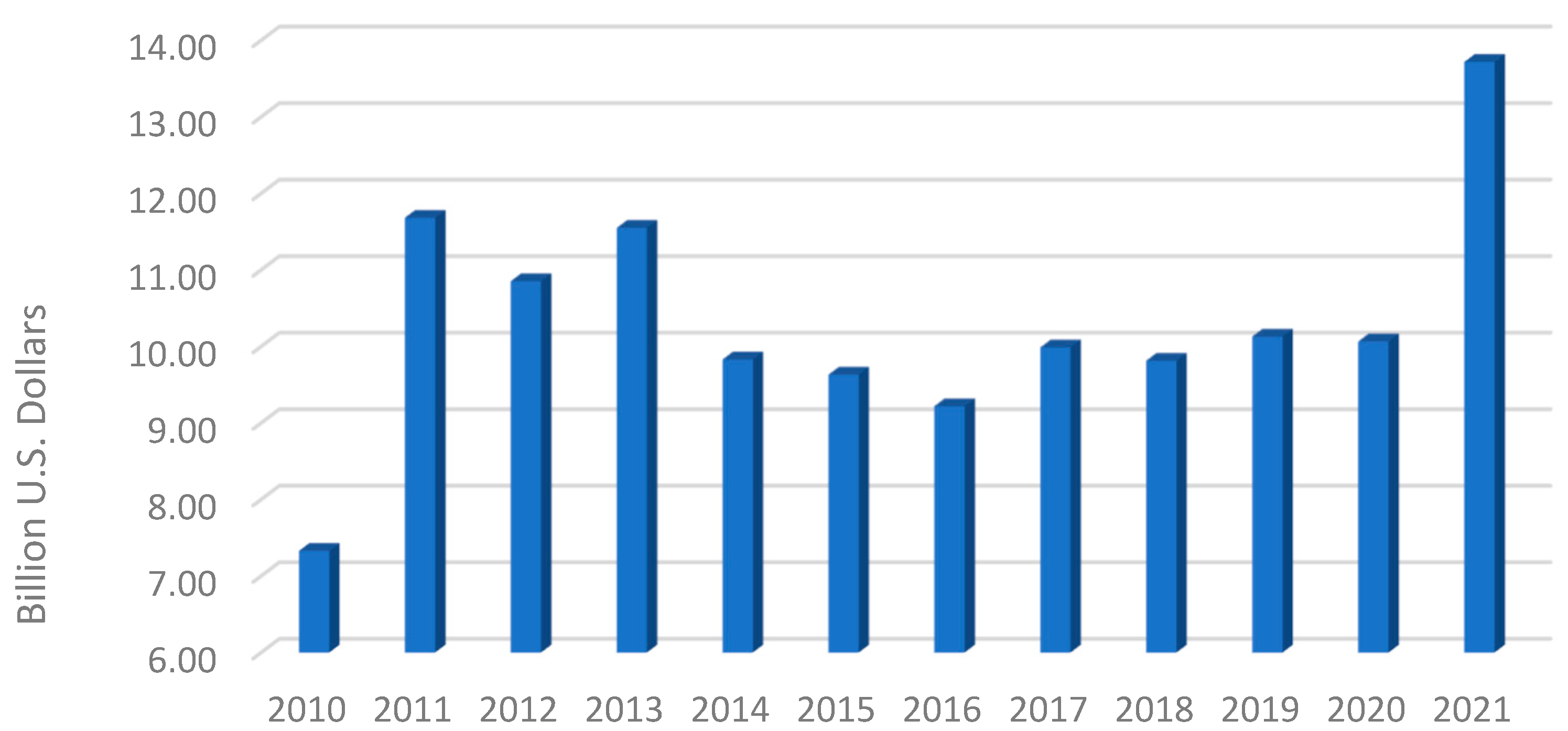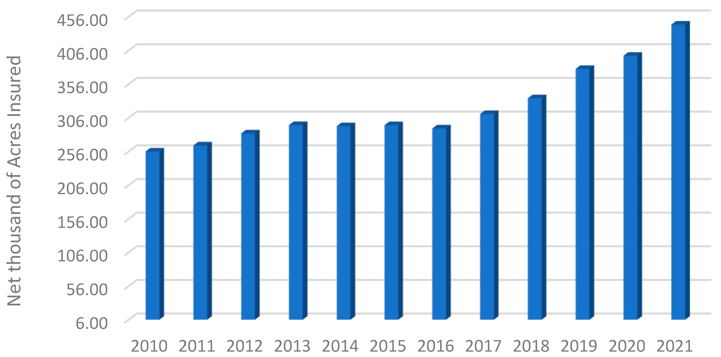Figure 2 and Figure 3 provides the graph of total agriculture insurance (Billion U.S. Dollars) and total area insured respectively.

Farmers in areas with high levels of air pollution need to limit their usage of pesticides to boost their yields and reduce environmental pollution. Farmer excitement for using fertilizer and pesticides can be stifled by the agricultural insurance system’s adverse selection and moral hazard, which reduces pollution [20]. Air pollution can diminish agricultural output; however, farmers may be encouraged to use more efficient and ecologically friendly green agricultural technologies by securing their financial futures via agricultural insurance, which affects AGTFP [21]. The United States has recommended agricultural insurance plans to safeguard agricultural productivity, reduce farmers’ air-pollution-related economic losses, and promote sustainability of rural growth. Agricultural insurance has been highlighted as a crucial instrument for aiding farmers, herders, and governments in mitigating the severe financial effects of natural disasters. Evidently, many nations have used insurance to mitigate agricultural hazards [22]. Agriculture insurance offers a way to reduce volatility, strengthen resilience, and support productivity growth in the agriculture sector—a sector that provides livelihoods to billions, food security to everyone, and stability to entire economies [23]. There are always going to be inherent risks associated with crop development, such as climate change and air pollution, and the most direct way to manage these risks is to establish scientific agricultural insurance policies, despite the fact that this has not been formally implemented anywhere in the world [23]. In addition, agricultural insurance may lessen the impact of smog, rainstorms, and other natural catastrophes on agricultural productivity, as well as increase farmers’ capacity to manage the risks associated with agricultural production [24]. This capacity to withstand risks might also inspire farmers to use environmentally friendly agricultural technology more aggressively in order to boost the productivity of their operations [23]. It has been brought to light that the use of environmentally friendly agricultural technology has the potential to greatly boost agricultural green total factor production. Thus, agricultural insurance has a significant correlation with agricultural green total factor productivity. The study considers the multiple peril crop insurance (MPCI) in which losses to crops, including decreased yields, that are incurred due to natural occurrences such as destructive weather are covered by MPCI (hail, frost, damaging wind). The MPCI is backed and controlled by the federal government, but it is marketed and serviced by crop insurance firms and brokers operating in the private sector. More than 90% of farmers who purchase crop insurance go with MPCI as their provider of choice. The worth of the particular crop determines not only how much an insurance policy will cost but also how much an insurer will pay out in the event of a loss [25].

This study article investigates the effect of air pollution and agricultural insurance on agricultural green total factor productivity (AGTFP). To assess AGTFP, the undesirable outputs model was selected, and the panel autoregressive distributed lags model was created to examine the impacts of air pollution and agricultural insurance on AGTFP. The study uses panel data from 50 US states from 2005 to 2019. This research makes some significant new additions to the literature. No similar research has been undertaken in the United States. Second, there is no mechanism through which agricultural insurance and air pollution directly influence agricultural green total factor production, and this article addresses this gap. Third, our study is connected to the factors influencing agricultural green total productivity. Green technological innovation, according to [26], may minimize pollution to the ecological environment caused by energy use and subsequently boost green total factor productivity. The United States’ green total factor productivity may be considerably affected at the regional and national levels by land transfer marketization, as demonstrated by [27]. This study differs from the others by focusing on green total factor productivity in agriculture. Last but not least, this research makes valuable policy recommendations for increasing the productivity of agricultural green total factors in the United States. This study proposes new ideas for improving AGTFP and encouraging the growth of green agriculture based on a fresh research approach.

The remaining sections of this article are as follows: Section 2 discusses the literature review. Data sources and the econometrics methodology are discussed in the third section, empirical results and discussion make up the fourth section, and the conclusion and policy recommendation will be discussed in the final section.

2. Literature Review

The majority of the research that has been completed so far has been on the factors that affect agricultural total green factor production. Stochastic boundary analysis and the Malmquist index approach were used by [26] to explore and discover that green production technology innovation may lessen the negative effect of fossil energy combustion residues on air pollution and boost green agriculture total factor productivity. The researchers came to this conclusion as a consequence of their findings that cutting-edge environmentally friendly manufacturing equipment has the potential to lessen the detrimental effect that leftovers from fossil fuel burning have on air pollution. Both [16] and [28] are of the opinion that the share of agricultural output value, as well as the agri-industrial structure, are essential elements that influence China’s AGTFP. In addition, the commercialization of land transfers and the advancement of internet technology has the potential to boost AGTFP, whereas the distortion of the factor market has the potential to impede the growth of AGTFP [27,29,30].

A significant increase in the rate of rural industrialization and urbanization would produce many pollutants, including PM2.5. According to refs. [31,32], the primary source of environmental health concerns is air pollution, and a more significant concentration of PM2.5 will increase the severity of this problem. In addition, rural regions have inadequate systems for managing agricultural residue. The primary method for disposing of crop residue is burning, which results in the emission of significant pollution levels in the atmosphere. For instance, northern China’s crop harvesting and burning operations emit around 10 tons of PM2.5 annually [33]. Extremely high levels of air pollution will have a wide range of unfavorable consequences, including the fact that it will disrupt the natural biochemical processes in plant tissues, reducing crop productivity and hastening the deterioration of soil quality [34]. The authors of Zivin and Neidell [35] also demonstrated that increased levels of air pollution might eventually result in a reduction in the effectiveness of agricultural output and labor productivity.

Agricultural insurance, on the other hand, perfectly transfers the risk associated with agricultural output. On the one hand, there are always risks in crop development, such as air pollution and climate change. Establishing scientific agriculture insurance coverage is the most straightforward method to control these risks; nevertheless, this strategy has not yet been legally adopted anywhere around the globe [23]. Moreover, agricultural insurance can also lessen the impact of smog, thunderstorms, and other natural catastrophes on agricultural productivity. It can also increase farmers’ ability to deal with the risks associated with agricultural production [24]. This ability to withstand hazards might also inspire farmers to use environmentally friendly agrarian technology more aggressively to boost their operations’ productivity [23]. It has been argued that implementing environmentally friendly agricultural practices can significantly raise agricultural green total factor production [36,37]. In addition, agricultural insurance can encourage farmers to employ biological pesticides rather than chemical pesticides, which results in minor environmental damage and is, thus, helping the growth of green agriculture [23]. Therefore, the association between agricultural insurance and AGTFP is statistically significant [25].

Li, Tang [8] conducted a study to investigate the relationship between agriculture insurance and air pollution. The author collected data for the time period of 2005–2019. By employing the panel vector auto-regressive method they concluded that to a certain degree, a rise in agricultural insurance may reduce air pollution.

Tang and Luo [38] investigate the association between agriculture insurance and the use of biological pesticides in three provinces of China. The paper employs the endogenous probit model and concluded that if agriculture insurance is provided to all the farmers the use of biological pesticides will be increased by 8.2%. The authors come to the conclusion that agriculture insurance can significantly reduce pollution by using biological pesticides and reduce the use of chemical pesticides.

Fang, Hu [25] examined the impact of agriculture insurance on agriculture green total factor productivity. The paper employs the SBM-GML index using data for the time period of 2002–2015. Their results found a significant impact of agriculture insurance on agriculture green total factor productivity.

Sehrawat and Giri [39] using yearly data from 1984 to 2013, explore the link between financial development indices and human capital for Asian nations. The stationarity of the variables is determined using the panel unit-root tests of Levin–Lin–Chu, Im–Pesaran–Shin, Fisher-type enhanced Dickey–Fuller, and Philips–Perron. Using Pedroni’s and Kao’s panel co-integration methods, the long-run connection between the variables is examined. Panel dynamic ordinary least squares (PDOLS) and completely modified ordinary least squares (FMOLS) are used to estimate the coefficients of co-integrating vectors. Panel Granger causality is used to analyze the short- and long-term causation.

Comparing AGTFP for 93 countries between 1980 and 2000 using a Malmquist index and data envelopment analysis was the focus of the study in [40], which was based on the FAO (DEA) data. Inputs and outputs can be aggregated through a distance function with the help of the Malmquist index approach, which does not need price data. The findings indicate that agricultural TFP development was robust in all countries before the year 2000, with some indication of catch-up occurring between low-performing and high-performing countries. The Malmquist index method was also utilized by [41] to estimate total factor productivity (TFP) growth for subsectors of the agricultural industry (crops as well as ruminant and non-ruminant livestock) for 116 nations between the years 1961 and 2006. According to the study’s findings, total factor productivity (TFP) development in developing nations and developed countries was diverging in the ruminant livestock sector while it was converging for crop and non-ruminant livestock production activities.

The Malmquist index approach has certain benefits, such as the fact that it does not require any price information to estimate TFP; nevertheless, it also has some drawbacks. In particular, it is sensitive to the group of nations being contrasted as well as the number of variables being accounted for in the model [42]. Estimates of TFP are likely to be plagued by measurement inaccuracies if they are not based on a representative sample of many nations. In addition, estimations produced using Malmquist index numbers frequently appear improbable [40,43], which might be because the implicit shadow prices derived for aggregation are based on unrealistic assumptions [40].

Because of these factors, superlative index techniques are favored over other approaches wherever accurate pricing data are available. The superlative index number approach is frequently used by national statistical organizations and is suggested by the OECD (2001) for collecting information on productivity.

To estimate and compare agricultural TFP growth across 171 nations, [44] utilized a Tornqvist index. Although data from the FAO were used, they were supplemented with a fixed set of average global prices from [45] to calculate revenue shares. To calculate cost-shares, the input elasticities were taken from country-level case studies. According to the research conducted by [44], the increase in agricultural TFP worldwide has sped up in recent decades, notably in emerging nations such as China and Brazil. This is in contrast to the most current projections of yield and labor productivity, both of which point to a slowdown on a worldwide scale [5].

3. Materials and Methods

This study collected data for agriculture insurance from the United States Department of Agriculture (Risk Management Agency) [19], including panel data for 50 states of the United States from 2005 to 2019. “Agricultural insurance is represented by per capita agricultural insurance income, and the value is the total agricultural insurance income ratio to the total rural population”.

Using data from NASA earth observation satellites and the Centers for Disease Control and Prevention [46], the Institute of Environment at Hong Kong University of Science and Technology developed a two-stage PM2.5 calculation model. The first stage uses aerosol optical thickness data from space remote sensing data, and the second stage uses this data to determine PM2.5 concentrations [47]. The second step is estimating the PM2.5 concentration on the ground based on the aerosol optical thickness data derived earlier [29]. The Atmospheric Composition Analysis Group at Dalhousie University in Canada made extensive geophysical estimations of PM2.5 by combining data from NASA satellites and ground-based monitoring stations [48]. The annual data of PM2.5 is available online [49] for the United States from 2005 to 2019. The PM2.5 matters are measured as micrograms (one-millionth of a gram) per cubic meter of air (µg/m³). As a result, you can rest assured that the data we chose regarding air pollution are accurate.

This research will follow the methodology of [50,51,52]. It will use data envelopment analysis to determine total factor productivity, considering a variety of inputs and outputs. Consideration given to the enhancement of production efficiency might concurrently reduce the emission of pollutants. We use undesirable results as output variables throughout the developmental testing phase of the efficiency. The term for this kind of effectiveness is AGTFP. The program Dea-Slover-Pro has two distinct variations of the unsatisfactory output model: the bad-output model and the non-separable model. We decided to use this bad-output approach, capable of dealing with both expected and unexpected output correspondingly. The specific SBM model with undesirable outcomes, such as carbon dioxide emissions, is known as the bad-output model, based on a modification of the standard SBM model. The SBM and Super-SBM models were utilized to evaluate completely effective decision units by [53]. Using the output model that produces undesirable results may be described as follows when based on the variable returns to the scale.

In this case, it is assumed that “m” is the input variable and “s” is the output variable, which includes desired and undesired outputs. $X=(x_1,x_2\dots )$ ∈ $R_m$ represents the input matrix and $Y=(y_1,y_2\dots )$ ∈ $R_s$ represents the output matrix. However, Y can be decomposed into $Y^g$ and $Y^b$, therefore, good and bad output matrices are represented by $Y^g$. and $Y^b$, respectively. Because it uses the non-directed model, the input and output data must be greater than zero, as mentioned earlier, and we set X, Y, $Y^g$, and $Y^b>0$. In this context, the DMUs’ production potential might be stated as follows:

$$P=\left\{\left(x, y^g, y^b\right)| x \ge X\lambda , y^g\le Y^g, y^b\le Y^b,L<e\lambda <U,\lambda \ge 0\right\}$$

(1)

where “Lower and upper limits” of intensity vector “L” and “U” have default values of 1 in DEA Solver Pro. “λ” is the intensity vector.

Every “decision-making unit” (DMU ($x_0,y^g,y^b))$. must have input and output data that meet the requirements in order to acquire the optimal frontier under a condition when an undesirable output variable is present. The requirements include: $x_0\ge x,y_0^g\le y^g,y^b$, and $\left(x,y^g,y^b\right)$ ∈ P. The undesirable output model is presented below in Formula (2):

$$\{\begin{array}{c}\mathsf{\rho }=min\frac{1-\frac{1}{m}{{\displaystyle \sum }}_{i=1}^m\frac{s_i^{-}}{x_i^0}}{1+\frac{1}{s_1+s_2}\left({{\displaystyle \sum }}_{r=1}^{s_1}\frac{s_r^g}{y_{r0}^g}+{{\displaystyle \sum }}_{r=1}^{s_2}\frac{s_r^b}{y_{r0}^b}\right)}\\ s.t.x_0=X\lambda +s^{-},y_0^g=Y^g\lambda -s^g,y_0^b=Y^b+s^b,L\le e\lambda \le U\\ s^{-}\ge 0, s^g\ge 0,s^b\ge 0,\lambda \ge 0\end{array}$$

(2)

where the insufficient desirable output of decision-making units, undesirable outcome, and an excess amount of input is represented by vectors $s^b,s^g,$ and $s^{-}$, respectively. The number of items in $s^g\mathrm{and}{s}^b$ are denoted by the values of the $s_1\mathrm{and}{s}_2$. In the context of bad output, the production efficiency may approach the optimal frontier domains if the following conditions were met: ρ = 0, $s^{-}=0,s^g=0,\mathrm{and}{s}^b=0$. Nevertheless, if 0 < ρ < 1, the efficiency of the unit that makes decisions is inefficient. Under the given conditions, we may discover helpful strategies to prioritize the scheme of its productive efficiency [54]. The main advantage of using Data Envelop Approach (DEA) is that it can handle a wide variety of inputs and outputs. When calculating efficiency, it is particularly helpful since it considers returns to scale. This allows for the possibility of increasing or reducing efficiency dependent on the size of the output level or the amount of the output [55].

The two components of AGTFP are agricultural input and output. Following Liao, Yu [56] agriculture input consists of labor, machinery, fertilizer, irrigation, and agriculture energy consumption. The agriculture labor is measured as workers per 1000 persons economically active in agriculture including both male and female individuals over 15 years old. Machinery is the measure of machinery used in farms measured with the metric horsepower (1000 CV) of farm machinery in use (includes tractors, harvester-threshers, and water pumps). Fertilizer is the measure of metric tons of fertilizers applied to soils. The output is composed of expected output and unexpected output. The expected output is the total output value of agriculture productivity and unexpected output includes agricultural carbon emissions.

This study considers the total agricultural output value after lowering the agricultural gross output value index to be the expected output. On the other hand, we think the carbon emissions created by various substances are an unexpected output. The methodology for calculating carbon emissions from agricultural practices will be discussed in more depth later.

The production of food or the use of a specific type of energy will result in the emission of a significant quantity of carbon dioxide, which will contribute significantly to the contamination of the natural environment [57]. For the most part, carbon dioxide emissions are to blame for environmental degradation and the rising average global temperatures [58]. At present, a significant number of publications have focused their attention exclusively on the computation of carbon dioxide emissions; nevertheless, the final findings computed by various categorization standards vary. Supposedly, in light of the carbon emission coefficient and the carbon sources of agricultural output, the following Formula (3) for measuring agricultural carbon emissions is constructed in this article:

$$E={\displaystyle \sum }{E}_i={\displaystyle \sum }{T}_i·{\delta }_i$$

(3)

where $“E”$ is the entire amount of carbon dioxide emissions caused by agricultural output. The $“E_i”$ is the amount of carbon that is emitted by a specific carbon variable. In this particular study, the variables on carbon sources that were utilized are the following: agricultural plastic film, agricultural pesticide, and chemical fertilizer, effective village area, the excrement from primary livestock including sheep, cattle, and pigs; rural electricity consumption, the irrigated area, and the agricultural diesel fuel consumption. The National Agricultural Statistics Service of the United States Department of Agriculture is the authority on all the farm input data presented above. The number of variables that are input is denoted by $T_i$.

The first and most significant step is to carry out a cross-section dependence test [59]. The weak cross-sectional dependency between variables is referred to as the null hypothesis. The study will reject the null hypothesis if the findings are significant, indicating a high cross-sectional relationship between agricultural insurance, the air pollution index, and agricultural green total factor productivity. This research uses the Pesaran Lagrange Multipliers test and the Pesaran CD test that was suggested by Breusch Lagrange multipliers and Pesaran in 2004. In the Pesaran CD test, an average correlation test is carried out on the variables based on the coefficient of the augmented Dickey–Fuller regression.

The vast majority of the macro index data do not remain stable at a certain level. In order to verify the variables’ consistency, data must be stationary at first-order difference [60]. The term “stability” refers to the consistency of the mean value, the standard deviation value, and the autocorrelation statistical structure of a collection of panel data over time [59]. In this investigation, we will use the Fisher-PP, the Fisher-ADF, the Pesaran and Shin test (IPS), and the Levin–Lin–Chu test.

The approaches developed by Pedroni [61] and Kao [62] are the ones that receive the most attention when testing the co-integration connection. Regarding panel data sets with a small-time dimension [63], Kao [62] can identify the particular section intercept and homogeneity coefficient of the first-order regression equation. The primary processes of the two tests are virtually the same. Therefore, we decided to use the co-integration relationship test technique after establishing a correlation between the variables at the cross-sectional level [62]. The Kao test is appropriate for use with bivariate data. It focuses on the exceptional circumstance of co-integral vector homogeneity between units [64]. The assumption that there is no co-integration connection that serves as the basis for the co-integration test based on the residual tests developed by Engle and Granger [65].

After establishing a co-integration relationship between the variables, we need to conduct additional research to determine whether there is a causal connection between agricultural insurance, air pollution, and agricultural green production efficiency. Green production efficiency will allow us to make policy recommendations that are more accurate and appropriate. A statistical hypothesis experiment known as the Granger causality test is a potent instrument for determining whether one series may accurately predict another series [66]. Suppose the prediction impact of the preceding sequence of x and y is better than that of the y sequence. In that case, the Granger causality test indicates a link between the variables in x and y [64]. Although the coefficients that are obtained using the PDOLS and FMOLS methods that are described below can provide an estimate of the long-term relationship between variables, they are not able to determine whether a causal relationship exists between the variables that are being explained and the variables that are being defined by them [67].

Third, to investigate the short-run and long-run impacts of air pollution and agricultural insurance on AGTFP, this study employed the pooled mean group–autoregressive distributed lag (PMG–ARDL) model developed by Pesaran, Shin [68]. According to Pesaran and Smith [69], the conventional approach, like GMM estimators, is considered inconsistent and potentially misleading unless the slopes are identical [70]. The advantage of using PMG-ARDL is that it estimates both short-run and long-run dynamics simultaneously; it supports multiple integration orders, notably level, first-difference, or a combination of both variables, as well as it allows for varying numbers of lags on each variable [71].

The specification of the PMG-ARDL model including the short- and long-run impacts is expressed as follows:

$$\begin{array}{c}{\mathrm{L}}_{\mathrm{TFP}}={\mathsf{\alpha }}_0+{\displaystyle {\displaystyle \sum }_{i=1}^r}{\lambda }_1{\mathrm{L}}_{\mathrm{TFPt}-1}+{\displaystyle {\displaystyle \sum }_{i=1}^r}{\lambda }_2{\mathrm{L}}_{\mathrm{PM}2.5\mathrm{t}-1}+{\displaystyle {\displaystyle \sum }_{i=1}^r}{\lambda }_3{\mathrm{L}}_{\mathrm{insurancet}-1}+{\mathsf{\sigma }}_1{\mathrm{L}}_{\mathrm{TFPt}-1}+{\mathsf{\sigma }}_2{\mathrm{L}}_{\mathrm{PM}2.5,\mathrm{t}-1}+{\mathsf{\sigma }}_3{\mathrm{L}}_{\mathrm{insurancet}-1}\hfill \\ \hspace{1em} \hspace{1em}\hspace{1em}\hspace{1em}\hspace{1em}\hspace{1em}+{\mathsf{\epsilon }}_{it}\end{array}$$

(4)

where ${\mathsf{\alpha }}_0$ denotes a constant term, $\lambda$ and $\mathsf{\sigma }$ represent the parameters in the short and long term, respectively. ${\mathsf{\epsilon }}_{it}$ represents the residual term.

This study further employs the “panel dynamic ordinary least square” (PDOLS) and “fully modified ordinary least square” (FMOLS), which are known for more robust results [67,72,73]. A nonparametric technique, the FMOLS method, offers the advantages of correcting simultaneous bias, sequence correlation, and correcting endoplasmic error [74]. The authors used the supplemental approach called DOLS in the long-term impact test to ensure that the test outcomes are accurate and reliable. The equations for FMOLS and PDOLS are expressed in Equations (4) and (5), respectively.

$${\widehat{\beta }}_{FMOLS}={\left({\displaystyle \sum }_{i=1}^N{\widehat{L}}_{22i}^{-2}{\displaystyle \sum }_{t=1}^T{\left(x_{it}-\overline{x}\right)}^2\right)}^{-1}{\displaystyle \sum }_{i=1}^N{\widehat{L}}_{11i}^{-1}{\widehat{L}}_{22i}^{-1}\left({\displaystyle \sum }_{t=1}^T\left(x_{it}-\overline{x}\right)y_{it}^{*}-T{\widehat{\delta }}_i\right)$$

(5)

where ${\mu }_{it}^{*}={\mu }_{it}-\frac{{\widehat{L}}_{21i}}{{\widehat{L}}_{22i}}\mathsf{\Delta }{x}_{it},$ ${\widehat{\delta }}_i={\widehat{\mathsf{\Gamma }}}_{21i}{\widehat{\mathsf{\Omega }}}_{21i}^0-\frac{{\widehat{L}}_{21i}}{{\widehat{L}}_{22i}}\left({\widehat{\mathsf{\Gamma }}}_{22i}+{\widehat{\mathsf{\Omega }}}_{22i}^0\right)$, and ${\widehat{L}}_i$ was the lower triangulation of

$${\widehat{\mathsf{\Omega }}}_i.{\widehat{\beta }}_{DOLS}=\frac{1}{N}\left[{\left({\displaystyle \sum }_{t=1}^T{Z}_{it}\ast Z_{it}^{\prime }\right)}^{-1}\left({\displaystyle \sum }_{t=1}^T{Z}_{it}\ast {\widehat{W}}_{it}\right)\right]$$

(6)

where $Z_{it}=\left[X_{it}-\overline{X_i},\mathsf{\Delta }{X}_{it-ki},\dots .,\mathsf{\Delta }{X}_{it+ki}\right]$ is vector of regressors and ${\widehat{W}}_{it}=W_{it}-\overline{W_i}$.

All of the collected data are first transformed into logarithm form. Among the numerous kinds of transformations used to alter skewed data to near normalcy, the log transformation is likely the most used. Another common use of the log transformation is to minimize data variability, particularly in data sets with outlier observations.

4. Results and Discussion

The results begin with

Table 1. Descriptive statistics.

Variables	Min	Mean	Max	Std. Dev.
Insurance	0	0.57879	9.52442	1.06275
AGTFP	0.07739	0.79461	1.09	0.17113
PM2.5	16.786	52.36033	99.408	19.05647

Source: Author(s) compilation.

which provides a descriptive statistic of the variables used in this study including the minimum and the maximum values, the average value, and the standard deviation.

The three factors that were chosen for this study all have some sort of connection to the production of agricultural goods. If the cross-sectional dependence is disregarded because of spatial factors or specific undiscovered cofactors, the consistency and unbiasedness of conventional panel estimators may be impacted [59]. These three approaches in

Table 2. The results of cross-sectional dependence tests.

Variables	Pesaran Scaled LM		Pesaran CSD		Breusch–Pagan LM
	Statistics	Prob. Value	Statistics	Prob. Value	Statistics	Prob. Value
lninsurance	131.15 *	<0.01	29.51 *	<0.01	1719.64 *	<0.01
lnAGTFP	141.35 *	<0.01	30.64 *	<0.01	789.52 *	<0.01
lnPM2.5	171.52 *	<0.01	41.22 *	<0.01	1892.61 *	<0.01

* denotes statistical significance at 1%. Source: Author(s) calculation.

are used to validate the findings of the cross-section dependency test in order to make the results of the test more accurate. The results shown in Table 2 demonstrate that the Breusch and Pagan LM test, the Pesaran scaled LM test, and the Pesaran CD test are statistically significant at the 1% level. The null hypothesis, which states that there is no cross-sectional co-integration connection, is rejected by all three methodologies.

Table 3. The LLC, IPS, ADF Fisher and PP Fisher chi squared tests.

Tests		Series
		Lninsurance	lnPM2.5	lnAGTFP
LLC test	Level	<0.05	<0.05	<0.05
	1st diff	<0.01	<0.01	<0.01
Pesaran and Shin test	Level	<0.05	0.094	<0.01
	1st diff	<0.01	<0.01	<0.01
ADF-Fisher chi-square test	Level	<0.05	0.074	<0.01
	1st diff	<0.01	<0.01	<0.01
PP-Fisher chi-square test	Level	<0.05	0.017	<0.01
	1st diff	<0.01	<0.01	<0.01

Source: Author(s) calculations.

provides the outcomes of the unit root test, including LLC, IPS, and two Fisher types of unit root test.

In accordance with the level requirements, the variable agriculture insurance is statistically significant at the level. Moreover, it is clear from the findings presented in Table 3 that the PM2.5 statistics are not reliable, with the exception of the tests conducted using the LLC technique, the findings of which do not include a unit root. Furthermore, the statistics of AGTFP held up well in the test conducted using the IPS technique. We re-tested the data once the first-order difference processing had been completed in order to ensure that the findings of the panel unit root test were consistent. In conclusion, we came to the realization that the outcomes of the unit root test applied to all the information were significant at the 1% level, which meant that the null hypothesis of sequence instability was refuted. The findings lead one to the conclusion that the panel data for air pollution, agricultural insurance, and AGTFP are stable in the first-order difference. Following the first-order difference, each and every data set is utilized in the empirical tests that come after it.

This study further employs the Kao [62] co-integration test to determine the existence of co-integration between factors such as air pollution, agricultural insurance, and AGTFP. Kao [62] put forward and tested the hypothesis that the data set in question does not include any co-integration relations. Moreover, the pairwise Granger causality analysis is estimated to test the causality relationship between the variables.

Table 4. Pairwise Granger causality analysis and Kao co-integration test.

Null Hypothesis:			F-Stat.	p-Value
Lninsurance	x->	Ln AGTFP	3.339	<0.01
Ln AGTFP	x->	Lninsurance	0.994	0.311
LnPM2.5	x->	Ln AGTFP	4.379	<0.01
Ln AGTFP	x->	LnPM2.5	0.991	0.337
LnPM2.5	x->	Lninsurance	1.125	0.178
Lninsurance	x->	LnPM2.5	4.809	<0.01
Kao’s test
		Null hypothesis	T-stat	p-value
		No cointegration	−3.167	<0.01

Note: x-> denotes no Granger causality; source: Author(s) calculation.

provides the outcomes of the Kao’s residual panel co-integration test, and the outcomes show that the aforementioned p-value is significant at 1%. The findings confirm the existence of a co-integration connection between variables.

Moreover, the findings of the pairwise Granger causality analysis provided in Table 4 shows that there is a one-way Granger causality association between agricultural insurance and AGTFP, air pollution and AGTFP, and agricultural insurance and air pollution. Increases in agricultural insurance have been shown to boost agricultural green total factor production and worsen air pollution. In contrast, high levels of air pollution do not boost the green total factor production in agriculture [75]. Alternatively stated, agricultural insurance could boost AGTFP both directly and potentially by lowering levels of air pollution. Achieving a win–win scenario between resource conservation and agricultural economic development is crucial, as is ensuring farmers’ income, and boosting agricultural green total factor productivity [8]. Total factor productivity improvement in agriculture has tremendous relevance for green production and long-term sustainability [25]. Agriculture insurance, which may properly limit the risk of agricultural output, is thus an essential instrument for contemporary agriculture. Agriculture insurance is an effective tool for mitigating economic risk and safeguarding agricultural output, but it also has the unintended consequence of decreasing pesticide investment due to moral hazard and adverse selection [38]. It has the potential to increase environmentally friendly agricultural output while also reducing resource waste and pollution. It is crucial that we raise the green total factor production in agriculture [22].

Agriculture green total factor productivity was shown to be affected by carbon dioxide emissions. Air pollution, especially carbon dioxide and nitrogen oxides, has been shown to have a significant detrimental influence on agricultural yields by biological research evidence [76,77,78]. Agriculture productivity is shown to decrease by 20–60% when exposed to pollution from urban areas as far as 15 km away [79,80,81]. Acid rain created by pollutants may damage soil by altering its chemistry or decreasing the concentration of vital plant nutrients. These results will add up over time and remain. Last but not least, new studies reveal evidence that air pollution has a detrimental influence on labor supply and productivity [82,83], mostly owing to its effect on human health. Carbon emissions and fine particulate matter (PM2.5) that settle on plants can disrupt the leaf’s natural respiration and photosynthetic processes. Chlorosis and death of leaf tissue may result from the combination of a thick crust and alkaline toxicity caused in rainy conditions due to PM2.5. The dust layer may also alter the effectiveness of agricultural chemicals sprayed onto plants. Soil pH can be adversely affected by the deposition of pollutants such as PM2.5, which can decrease agricultural green total factor productivity [84].

This study employed the pooled mean group–autoregressive distributed lag (PMG–ARDL) model developed by Pesaran, Shin [68] provided in

Table 5. Panel autoregressive distributed lag (ARDL) test (dependent variable log AGTFP).

Variable	Coefficient	Standard Error	Prob.
Short-run equation
COINTEQ01	−0.3556	0.05621	<0.01
D(LNINSURANCE)	0.0117	0.0971	<0.10
D(LNPM2.5)	−0.0075	0.0253	<0.10
Constant	0.1127	0.0478	<0.01
Long-run equation
LNINSURANCE	0.0121	0.0079	<0.01
LNPM2.5	−0.1132	0.0480	<0.01

Source: Author(s) calculations.

below.

The findings shown in Table 5 indicate that, over the course of time, the influence of agricultural insurance and the air pollution index on AGTFP is same as compared to the estimated outcomes produced by the FMOLS and PDOLS approaches. In the long term, agricultural insurance has a considerable significant influence on AGTFP. Varied crops have very different insurance coverage benefits. Increases have been made to the crop insurance premium, catastrophe compensation, and safety measures. However, despite the importance of protecting farmers’ livelihoods in the face of disaster, only a small percentage of food crops are insured, resulting in inadequate compensation [85]. Consequently, crop insurance promotes agricultural green total factor production more so in cash crops than in food ones. Large-scale farmers are more likely to invest in insurance to support environmentally friendly farming practices [86]. Large-scale operations are more likely to turn to credit after enrolling in insurance due to the high production costs and high availability of credit involved in doing so, all with the goal of raising the bar for agricultural green technology and bolstering green production [75]. Therefore, crop insurance has a more significant impact on advancing AGTFP than small-scale farming. Moreover, PM2.5 content has a large negative impact on AGTFP. Some plant stages are more vulnerable to PM2.5’s detrimental effects on agriculture’s green total factor production and, as a result, crop yields [87,88,89]. Agriculture production is decreased by PM2.5 because less sunlight reaches the crop, this considerable effect is seen in most of the agriculture products [90]. In the short term, there is no evident impact exerted by the two explanatory factors on the AGTFP [91]. The results are in line with the results of [90,92].

Lastly,

Table 6. Results of the PFMOLS and the PDOLS estimations.

Dependent Variable log AGTFP
PFMOLS				PDOLS
Series	Co-Eff.	t-Stats.	Prob.-Value	Series	Co-Eff.	t-Stats.	Prob.-Value
Lninsurance	0.029	4.958	<0.01	Lninsurance	0.058	4.781	<0.01
LnPM2.5	−0.112	1.957	0.041	LnPM2.5	−0.051	2.017	0.049

Source: Author(s) calculation.

provides the estimated results of the “panel fully modified ordinary least squares” (FMOLS) and “panel dynamic ordinary least squares” (PDOLS) models. Both tests provide the magnitude and sign of the long-run relationship between the selected variables.

The findings reveal that the coefficient of agricultural insurance is positive, whereas the coefficient of PM2.5 is negative. Furthermore, both agricultural insurance and PM2.5 are shown to be statistically significant at the 1% and 5% levels. According to the calculations of FMOLS and PDOLS, an increase of 1% in agricultural insurance will result in a rise of 2.9% and 5.8%, respectively, in the AGTFP. On the other hand, estimates of FMOLS and PDOLS show that an increase of 1% in PM2.5 content would result in a reduction of 11.2% and 5.1% in AGTFP, respectively. This indicates that the more air pollution there is in agriculture, the lower the yields are likely to be.

The aforementioned empirical findings make it abundantly evident that agricultural insurance and air pollution both have a significant effect on the AGTFP. Technology for the quick implementation of green development in the agriculture sector, the improvement of the rural living environment, preservation and exploitation of agricultural resources, and the progress made in the area of the agricultural standard system are the primary contributors to the United States’ progress in agricultural science. It has been stated that the primary contributors to variables impacting agricultural total factor productivity are the enhancement of production efficiency and the progression of technical advancement. To begin, a significant increase in the rate of productivity growth is one of the primary indicators that scientific and technical innovation is growing stronger. For the sake of achieving economic expansion, the United States is actively supporting the agricultural production technology innovation-driven development plan. Due to the improvement of agriculture’s technical base and influence of technological innovation on total factor productivity, agricultural production should embrace technological innovation and change to the fullest extent possible. This should be undertaken in order to realize the full potential of technological innovation and reform. Second, in recent years, the United States has placed a particular emphasis on the construction of an ecological civilization with the primary goals of environmental protection, emission reduction, and energy conservation. This has reduced the degree to which economic growth is dependent on the amount of energy that is consumed. The ecological quality of the United States as a whole is exhibiting a pattern of persistent improvement. For the purpose of combating climate change, the region must have fully implemented programs for avoiding and managing air and soil pollution, and it has aggressively encouraged environmentally friendly growth. The findings are consistent with the literature, i.e., Fang, Hu [25], which also reveals that farmers receive assistance with the adoption of advanced agricultural green technology through agricultural insurance, that production risks can be transferred, and that farmers’ incomes can be guaranteed in order to raise AGTFP.

5. Conclusions and Policy Recommendation

We examined the link between air pollution, agricultural insurance, and AGTFP in all 50 states of the United States from 2005 to 2019 using a panel autoregressive distributed lags model. Following the first-order difference processing, the data index sequence was found to maintain its integrity according to the empirical findings that we gathered. The study found a substantial cross-sectional dependence as well as a co-integration connection existing between the three primary variables. There is a one-way Granger causality between agricultural insurance and AGTFP, air pollution and AGTFP, and agricultural insurance and air pollution.

Agricultural insurance is the Granger causality of air pollution, and there is a one-way Granger causality relationship between air pollution, AGTFP, and agricultural insurance. Agricultural insurance is also the Granger causality of AGTFP. Furthermore, the expansion of agricultural insurance, when seen from the perspective of its influence over the long term, is beneficial for the enhancement of AGTFP.

In light of the findings presented above, the following policy recommendations for environmentally responsible agricultural growth are offered. (1) Step up the implementation of cutting-edge technology for food production in agricultural settings. Local agricultural universities or research institutions related to agricultural science will encourage agricultural workers to use cutting-edge environmentally friendly agricultural technology, and the effectiveness of resource utilization will be improved and will reduce the waste of resources. (2) Establish and develop a system of income support and security for farmers, as well as improve the insurance policy covering agricultural produce. This approach has the capacity to effectively spread and transfer agricultural production’s inherent hazards, the intentions of farmers in reference to their incomes, and agricultural insurance is both scientifically sound and economically viable, having the potential to boost agricultural total factor productivity and encourage the expansion of agriculture in a more environmentally conscious manner. (3) Decrease the amount of chemical and agricultural inputs, including pesticides and fertilizers, that are used in order to lower the number of pollutant emissions. In an effort to get farmers to utilize agricultural inputs that are less harmful to the environment, the government has increased the amount of money they spend on subsidizing organic fertilizers. The United States is only getting started on the path toward sustainable development. There is still a long way to go before achieving environmental protection, increased productivity, and the successful implementation of sustainable agricultural development via the combined efforts of all members of society.