Article

Identifying Field Crop Diseases Using Transformer-Embedded Convolutional Neural Network

School of Electrical and Information Engineering, Jiangsu University, Zhenjiang 212013, China
*
Author to whom correspondence should be addressed.
Agriculture 2022, 12(8), 1083; https://doi.org/10.3390/agriculture12081083
Submission received: 15 June 2022 / Revised: 15 July 2022 / Accepted: 21 July 2022 / Published: 22 July 2022
(This article belongs to the Topic Integrated Pest Management of Crops)

Abstract

:
The yield and security of grain are seriously infringed on by crop diseases, which are the critical factor hindering the green and high-quality development of agriculture. The existing crop disease identification models make it difficult to focus on the disease spot area. Additionally, crops with similar disease characteristics are easily misidentified. To address the above problems, this paper proposed an accurate and efficient disease identification model, which not only incorporated local and global features of images for feature analysis, but also improved the separability between similar diseases. First, Transformer Encoder was introduced into the improved model as a convolution operation, so as to establish the dependency between long-distance features and extract the global features of the disease images. Then, Centerloss was introduced as a penalty term to optimize the common cross-entropy loss, so as to expand the inter-class difference of crop disease characteristics and narrow their intra-class gap. Finally, according to the characteristics of the datasets, a more appropriate evaluation index was used to carry out experiments on different datasets. The identification accuracy of 99.62% was obtained on Plant Village, and the balanced accuracy of 96.58% was obtained on Dataset1 with a complex background. It showed good generalization ability when facing disease images from different sources. The improved model also balanced the contradiction between identification accuracy and parameter quantity. Compared with pure CNN and Transformer models, the leaf disease identification model proposed in this paper not only focuses more on the disease regions of leaves, but also better distinguishes different diseases with similar characteristics.

1. Introduction

Gu et al. [1] predict that the global grain industry will face huge impacts from all aspects in 2030. How to guarantee the green and high-quality developments of agriculture will be one of the focuses of future agricultural work. The occurrence and spread of crop diseases are hard to predict, so timely early warnings and prevention are of extraordinary significance to crop yield and quality [2]. However, up to now, recognizing diseases by experienced experts is still the main approach in this field, which is time-consuming and laborious. To some extent, it is ineffective in controlling the occurrence, spread and damage of diseases [3,4,5]. Consequently, an automatic, less laborious and efficient method is highly desired to ensure high crop yield and quality. Along with the developments and improvements of computer vision technology, image classification and target detection technology based on convolutional neural network (CNN) provides a new way for crop disease management. It is different from traditional methods, with its ability to efficiently process massive data and learn target features (including color, texture, edge and other features) [6,7,8]. However, some problems remain unresolved when using computer vision technology to identify crop diseases. For example, in a complex environment, it is difficult for disease identification models to focus on disease spots, especially on small areas, which are not conducive to the early identification of crop diseases; different diseases may have similar characteristics, and the model may make wrong judgments when facing similar characteristics. Therefore, aiming at the above problems, this paper proposed to introduce Transformer Encoder into CNN to establish the relationship between long-distance features, so as to make up for the deficiency of the CNN model in extracting global features. In addition, Centerloss was introduced as a penalty term to optimize the common cross-entropy loss, so as to expand the inter-class difference of crop disease characteristics and narrow their intra-class gap.
The remainder of this paper is introduced as follows. Section 2 shows the research results of crop disease identification. Section 3 presents the datasets applied in this paper and the optimization details of the disease identification model. Section 4 introduces the experimental results and discussion. Section 5 summarizes the paper.

2. Related Work

Ashwinkumar et al. [9] separated the diseased and healthy regions of leaves based on Kapur’s thresholding, and utilized an emperor penguin optimizer algorithm to search the parameters, and the optimal model with 98.5% recognition accuracy was finally obtained. Kamal et al. [10] proposed Reduced MobileNet with few parameters, which effectively weighed the relationships between latency and performance. Ji et al. [11] combined the width features of Inception-V3 with the depth features of ResNet-50 to enhance the representation of target features, and conducted experiments on grape datasets containing four diseases. Sun et al. [12] added batch normalization and global pooling to AlexNet and obtained a new model with rapid convergence. Six models were finetuned and evaluated by Too et al. [13]. Among them, parameter quantity and running time of DenseNets-121 were more reasonable, and no performance degradation and overfitting occurred during training. Zhao et al. [14] conducted transfer learning based on a pretrained model on cotton datasets, which alleviated the overfitting problem of the original model. Mohameth et al. [15] compared the advantages and disadvantages of traditional machine learning and CNN, discussed the effects of transfer learning and feature extraction of multiple layers on recognition performance, and selected VGG16 for training. As far as the results are concerned, the performance of their proposed model is excellent. However, they only considered the effect of model structures on the results and ignored the association between disease features. Mohanty et al. realized the importance of the generalization performance and tested the model using other similar disease images, and finally obtained satisfactory results. However, Mohanty et al. [16] also failed to do further analysis of the disease features and simply fed the images into the model to obtain the results. In addition, Mohanty et al. failed to achieve a good balance between recognition accuracy and number of parameters. Huang et al. [17] proposed a neural architecture search network and performed extensive preprocessing operations on the dataset, which eventually obtained excellent results. However, the network takes some time to search for the best parameters and is not flexible enough.
Although the aforementioned studies have demonstrated excellent results in the field of crop disease recognition based on the convolutional neural network, the datasets they used only contained a single diseased leaf and a simple background. The disease features extracted and learned by CNN on such datasets are insufficient, which directly leads to the unsatisfactory generalization ability of models. Therefore, researchers have gradually shifted the focus of follow-up work to leaf disease data in complex environments and complex backgrounds. A Complex environment means the image contains different light intensity, noise and other disturbing factors, and complex background means the image contains sky, soil, multiple leaves and other backgrounds.
In response to the problem of poor recognition effect of some models, Gao et al. [18] used ResNet as the basic architecture and took feature differences among diseases as the entry point to solve the problem, and the ability of extracting adjacent channel features and filtering key features was successfully enhanced. Finally, the model achieved a high accuracy of disease recognition. Zhou et al. [19] constructed a multimodal recognition model incorporating image and text information to compensate for the low credibility and poor interpretability of image information, and the recognition accuracy with 99% was attained on private datasets. Picon et al. [20] applied three different CNN architectures on the crop disease datasets obtained in a real environment to simulate the disease identification work under complex backgrounds, and the recognition performance of models was improved by fusing the contextual information of plant diseases. Whereas recognition accuracy is certainly an essential metric to evaluate the performance of the model, the quantity of parameters is also critical if we are to port the model to mobile devices. With the purpose of simplifying structures and enhancing the ability of extracting micro disease features, Chen et al. [21] proposed a lightweight model based on transfer learning. Although the improved model had high performance, its applicability was poor, so it cannot be flexibly used in different tasks. Wang et al. [22] significantly reduced the parameter quantities and storage space of the model by changing the residual connection mode and using group convolution, and finally a faster speed was obtained when identifying tomato and cucumber diseases in the field. In addition, Tang et al. [23] added attention mechanisms to ShuffleNet-V1 and ShuffleNet-V2, which can improve parameter utilization and realize high-quality spatial coding. The improved models had high real-time performance in identifying leaf diseases. In addition, we have made some comparisons with some of the above literatures, and listed them in Table 1.
All the aforementioned studies targeted crop leaf diseases in complex environments, and provided theoretical guidance for disease management from the perspective of recognition accuracy as well as model landing [24]. CNN, as a tool used in the studies to extract disease features and identify disease categories, enhances the expression ability of features through the connection relationship among layers. By virtue of its shared convolution kernel parameters, redundant computations are avoided and the computational efficiency is improved. However, due to the ‘moving window’ attribute of convolution kernels, CNN still has some limitations in capturing global features. Inspired by the Transformer [25], and more specifically by the Transformer Encoder mechanism [26], this study proposed a disease recognition model combining CNN and Transformer. The model proposed in this paper aims to solve the problems in the process of crop disease identification in complex environment. Firstly, the proposed hybrid model made use of Transformer’s ability to capture the dependencies between remote features, so as to compensate for the deficiency of CNNs in diseases recognition, Secondly, for similar characteristics between different diseases, we improved the loss function so that the improved model can expand the distance between classes, reduce the distance within classes and reduce the misclassified disease characteristics. Finally, for the unbalanced sample size, we adopt a more appropriate balance accuracy rate to mitigate the impact of this problem on the final recognition results. In addition, different from the general hybrid models, this model is a lightweight visual task processing network, and it has fast image processing speed.

3. Materials and Methods

In response to the deficiency of CNN to extract global features of images, Transformer, which is capable of establishing dependencies between remote features, is introduced. That is, the parameter quantity and the processing efficiency of the improved model will be effectively optimized. Meanwhile, the global features extracted by Transformer will benefit from inductive bias of CNN. In this study, the above improved methods were proposed to realize the efficient identification of diseased leaves in complex environments.

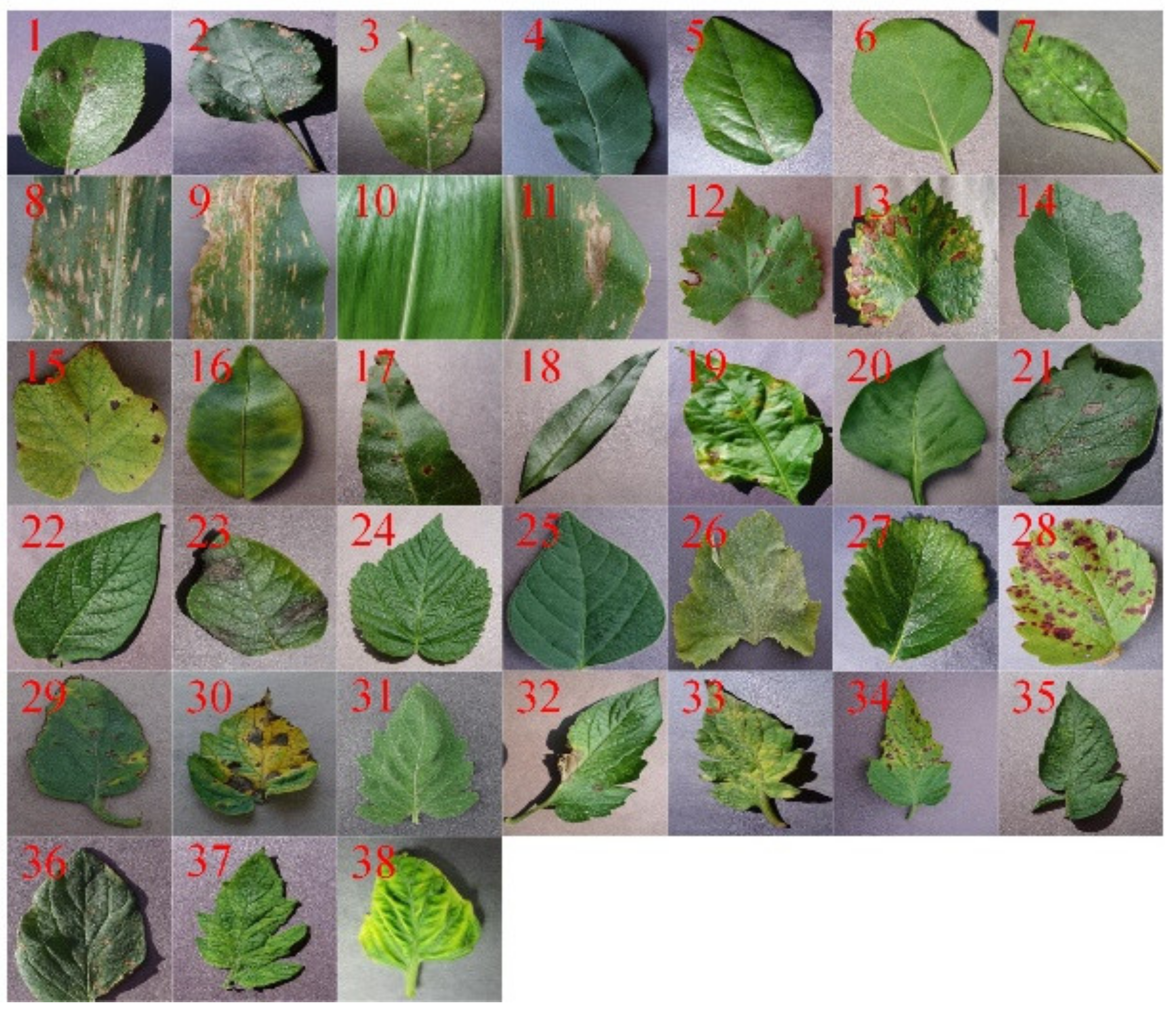
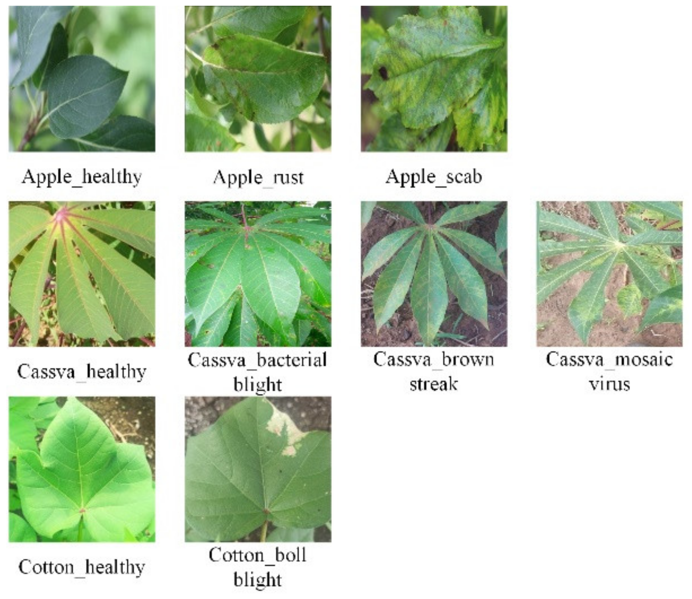
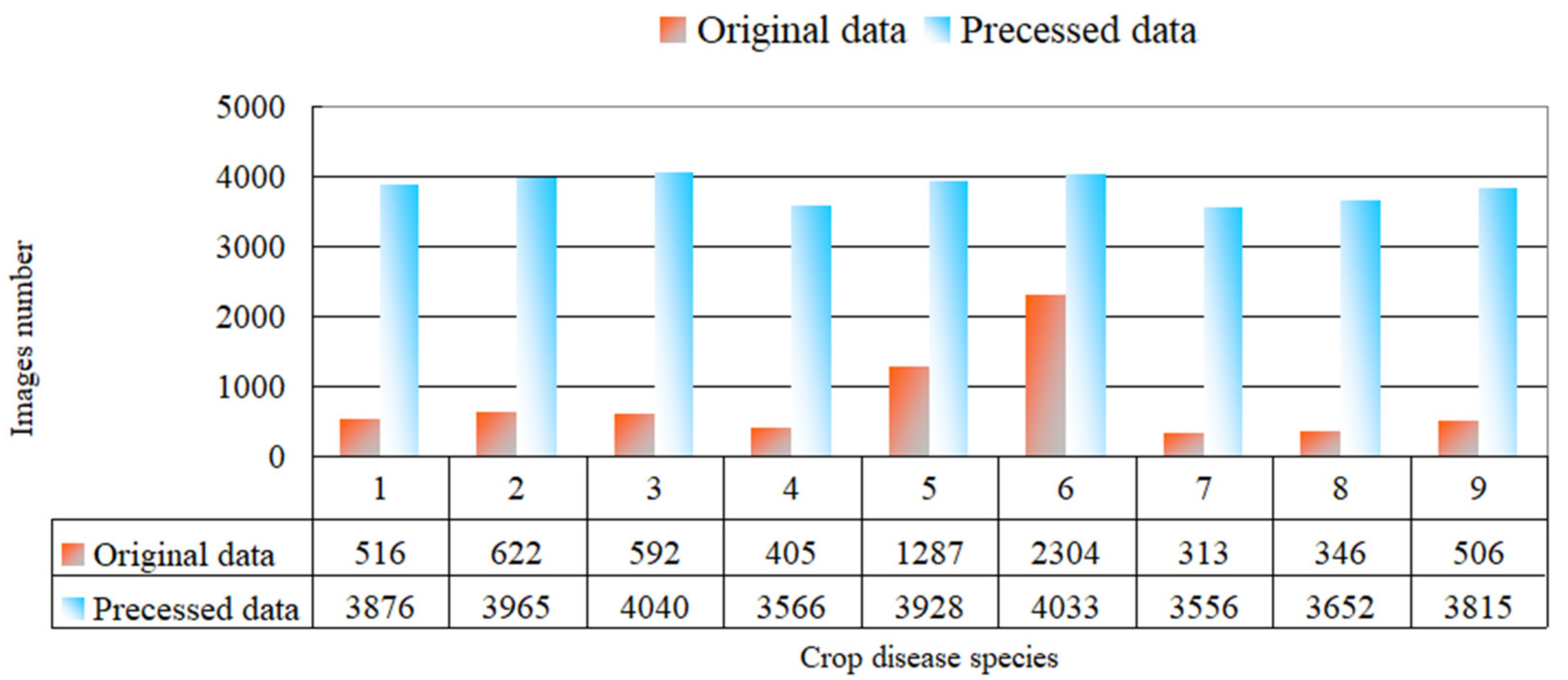
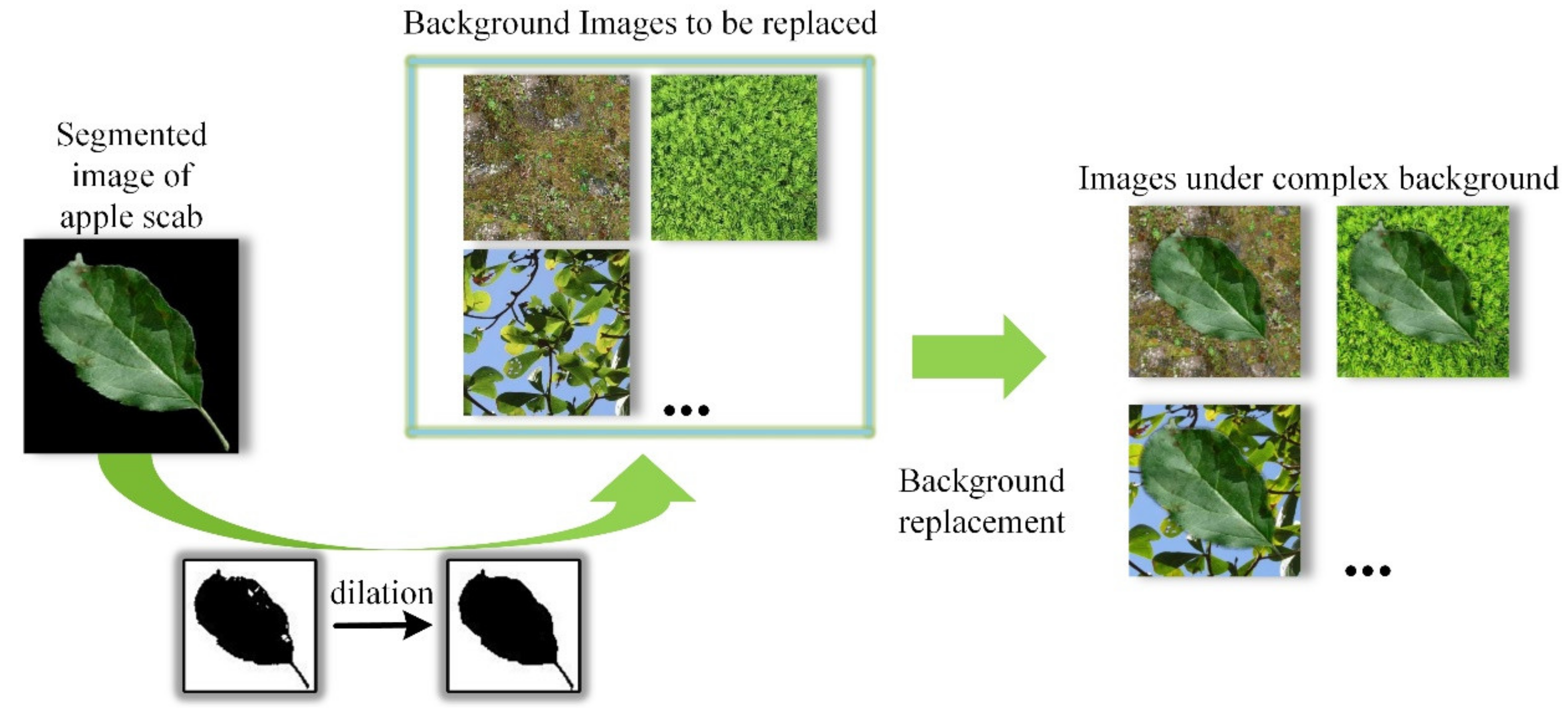
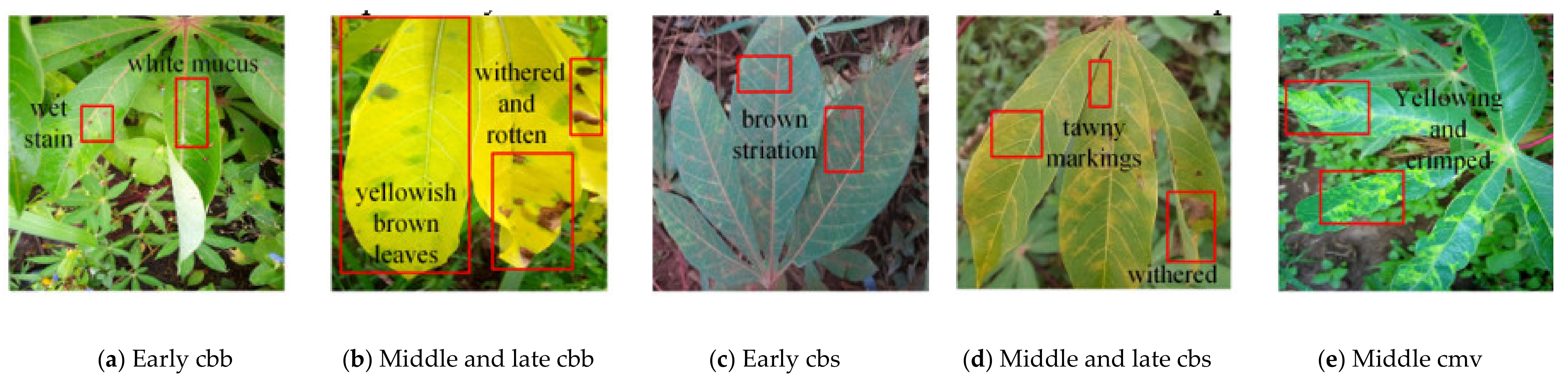
3.1. Datasets Acquisition and Preprocessing

As displayed in Figure 1, the public dataset from Plant Village [27], which contains healthy leaves of 14 crops and 24 types of diseased leaves, was prepared as a common benchmark to measure the differences in performance among different models. Meanwhile, considering the problem of harsh environmental disturbance in disease recognition in the field, two additional crop leaf disease datasets with complex backgrounds were prepared. The original images of Dataset1 (containing apple, cassava, cotton) were obtained from Kaggle [28], and leaf samples are shown in Figure 2. There are only 6891 unevenly distributed images in the initial Dataset1. This would not only make the categories with large number accumulate more errors in multiple iterative training, but also lead to some negative effects on the models such as overfitting and poor generalization performance [29]. Therefore, data enhancement operations including random rotation and brightness were applied to Dataset1 [30,31], and the number of images in each category before and after enhancement is given in Figure 3. Training data from the same source may result in poor generalization performance of the final model, which is detrimental for identifying crop diseases in different regions. In addition, without the guidance of professionals, it is difficult for us to obtain the corresponding pictures of crop diseases, which requires us to explore the existing data. Thus, we need to use background replacement technology to generate new data on the basis of existing data. The background replacement technique can simulate the recognition scenarios of different environments by replacing the background of the images based on the existing data. It is efficient and accurate for the whole experimental process.
Dataset2 contains images of apple scab, cassava brown streak and cotton boll blight, which was derived from the segmented leaf images in other datasets. The method in Figure 4 was used to replace its single background. We replace the background based on OpenCV in Python. Briefly, background replacement is to embed a single leaf into other complex backgrounds. Therefore, we need to remove the black background in the original image and obtain the binary mask of the leaf in the image to perform background replacement. Specifically, first we converted the RGB images to HSV images. Since the background of the original image is black, the threshold value of black corresponding to the HSV color space is (0,0,46). Therefore, we pre-set the threshold range that separates the leaf from the black background according to (0,0,46), and then obtain the binary mask image of the green leaf (a value of 0 for black corresponds to the leaf and a value of 255 for white corresponds to the background). However, due to the dark spots on the leaves, which are similar to the black background, several white spots appear in the leaf area in the mask image acquired at the beginning. In order to obtain a complete single leaf, we need to eliminate the white spots in the leaf area. We thus apply a morphological open operation consisting of erosion and dilation in sequence to get the final mask. Eventually, different complex backgrounds (soil, branches, multiple leaves, etc.) are selected to replace the background.
The above two datasets were used in different ways. Dataset1 was divided into the training set and test set by 4:1, which was used for model training and testing, respectively, whereas Dataset2, with a total of 2160 images (each category contains 720 images), was only regarded as a test set, mainly for studying the generalization performance of the models.

3.2. MobileNet-V2

At the early stage of CNN’s development, the convolution layers and pooling layers were continuously stacked to increase the depth of the models, so as to learn the target characteristics at different abstract levels. For example, residual connections were proposed in ResNet [22] to extend the layer number of the model from the initial 18 layers to 50, 101, or even 152. Although the design of stacked layers can obtain a larger pixel range by enlarging the receptive field, computational cost and parameter quantity of the model will also rise, which is unfavorable to the field recognition of diseases. The intensive nature of crop cultivation and the hidden location of diseases make it necessary for growers to still work with mobile devices to identify diseases on the scene. However, ordinary large models are hard to adapt to mobile devices with limited computing resources [32,33]. Hence, the degree of lightweightedness is the basis of intelligent disease recognition. In 2019, the lightweight MobileNet-V2, which can be deployed on portable devices, was proposed by Sandler et al. [34]. Firstly, the depthwise separable convolution in MobileNet-V1, which was proposed to reduce the number of convolutional kernels and speed up the model operation, was inherited by MobileNet-V2. Secondly, aiming at the design of the traditional bottleneck layer (reducing the dimension first and then increasing the dimension), Inverted Residual Block (IRB, ascending first and then descending) in Figure 5 was proposed, which not only significantly reduced the memory required during model inference, but also ensured that the rich feature information can be received by the Depthwise Convolution (DWConv) layer of IRB. Finally, in order to solve the problem of feature loss when high-dimensional features were compressed into low-dimensional features, the nonlinear activation function ReLU6 in MobileNet-V2 was changed into a linear function, so as to retain the diversity of feature information and enhance the expression ability of target features.

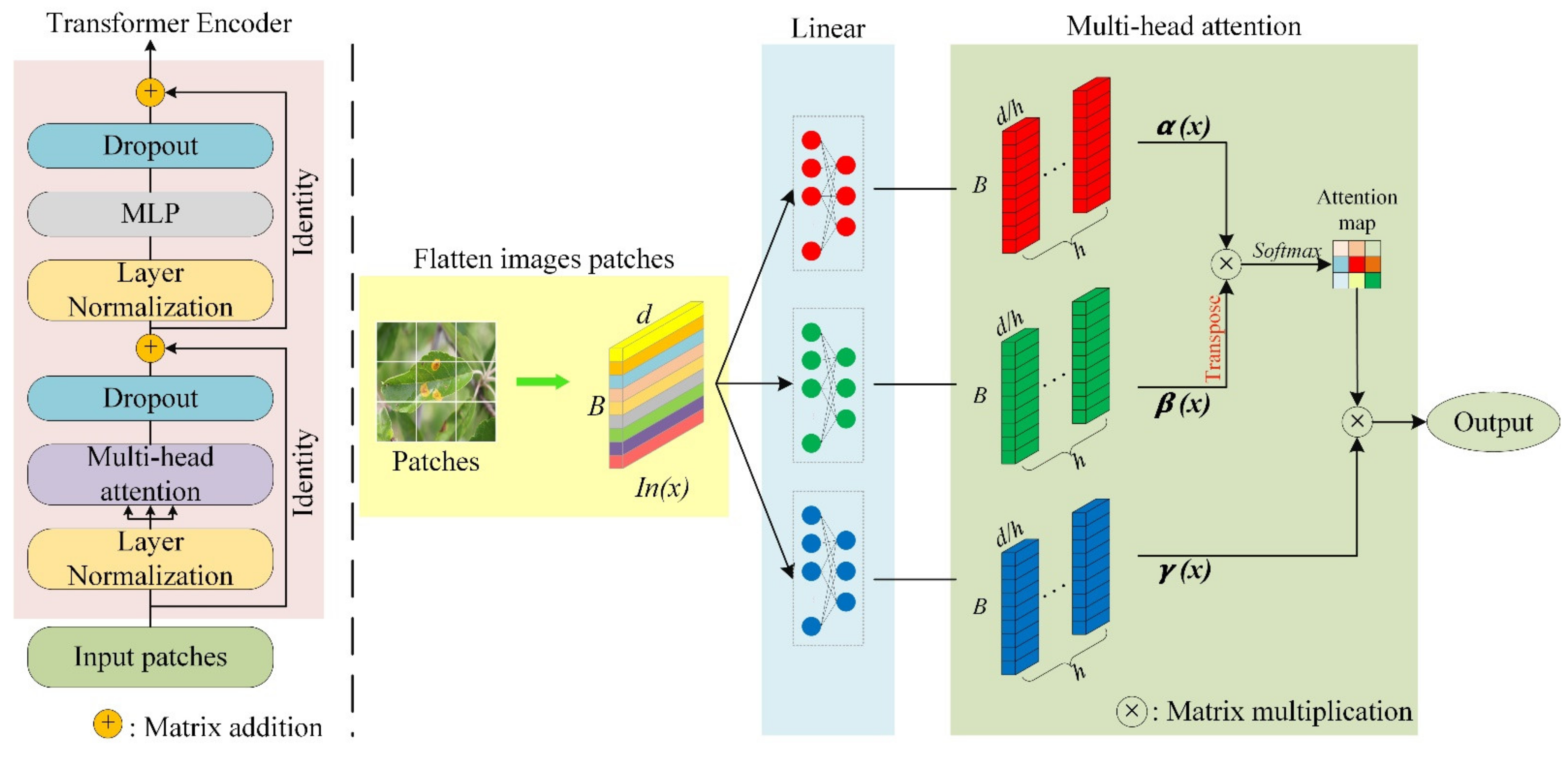
3.3. Transformer Encoder

The standard Transformer Encoder is composed of 4 basic units, as illustrated on the left side of Figure 6. The input data is normalized by Layer Normalization to accelerate convergence. Dropout is to prevent overfitting and improve the generalization ability of models. MLP can be simply understood as the stacked linear mapping operations. However, what really sets Transformer apart is Multi-head attention, as illustrated on the right side of Figure 6. The input I n x B × d is processed in parallel, when h = 1, α x ,   β x ,   γ x B × d can be obtained, respectively. Obviously, the above process can be summarized as Equation (1).
α x = I n x W α ,     β x = I n x W β ,     γ x = I n x W γ
where W α ,   W β ,   W γ d × d are three different parameter matrices, d is the length of input sequences and B is the number of input sequences. Since the same dimension is shared with α x and β x , they cannot be multiplied by each other. To meet the requirements of matrix multiplication, β x will be transposed. Subsequently, Softmax is performed on the multiplication results to obtain the attention degree A M i j of all feature points to a certain feature point, and the attention map can be formed by several A M i j . Ultimately, the output of the entire module was constituted by the fusion result of attention map and γ x . The above processes can be calculated by Equation (2).
S o f t m a x :   A M i j x = e x p F i j i ,   j = 0 B e x p F i j w h e r e   F i j = α x i     β x j T A t t e n t i o n ( x )   =   A M ( x )       γ x
∗ denotes the matrix multiplication operation. When h = 2, the whole process can be obtained from Equation (3) [35].
M u l t i h e a d = h e a d 1 , , h e a d h W o w h e r e   h e a d h   =   A t t e n t i o n ( x W s )
W s d × d h , W o d × d , h denotes the number of groups. Equation (3) can be understood as dividing the long input sequence into several short sequences of equal length, and feeding them into different Head Attentions, respectively, so as to more comprehensively mine the information generated by the features at different locations in different spaces.

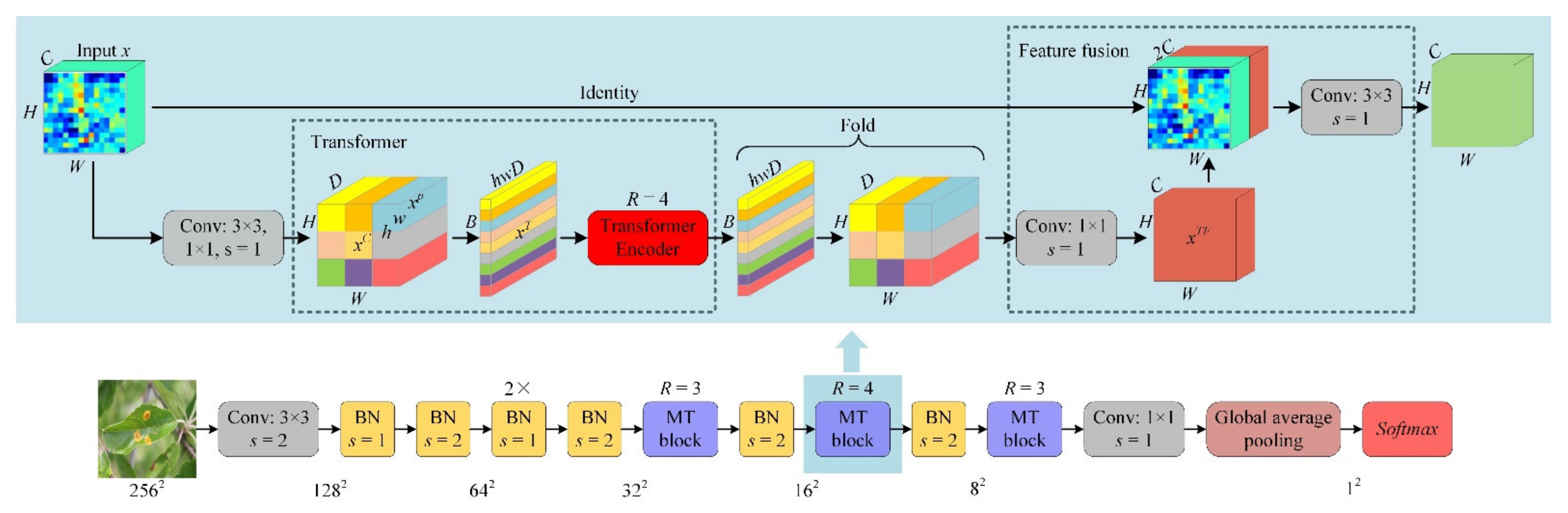
3.4. Proposed Hybrid Model

The images of crop leaf disease collected in the field have complex backgrounds, diverse characteristics and disorderly distributed disease regions. Faced with such images, the local features extracted by CNN often cannot completely represent certain diseases. Consequently, combined with Transformer’s ability to extract global features of images, a hybrid model combining CNN and Transformer was proposed, as illustrated in Figure 7. MobileNet-V2 is taken as the basic network in this hybrid model. First of all, a 3 × 3 convolution kernel is used to reduce the size of the input disease images, and the retained valid information will be mapped to a higher dimensional feature space. In the second place, in order to acquire more abundant disease feature information, meet the requirements of Transformer Encoder for input size and improve the overall processing efficiency of the model, the feature information is continuously input into the IRBs of MobileNet-V2 for multiple nonlinear transformations and size reduction. The most important is the Mobile-Transformer block (MT block, see Figure 7). As can be seen from Figure 7, for an input x H × W × C , a 3 × 3 convolution kernel is used for encoding, a 1 × 1 convolution kernel is used to expand the dimension of encoded feature maps to obtain x C H × W × D (D > C), and x C H × W × D will be divided into B patches x p h × w × D (h = w = 2 are the length and width of the patch, respectively, and B is the number of patches, which can be calculated by H × W h × w ). Afterwards, in order to obtain the linear input x T B × h w D required by Transformer Encoder, we flatten each x p to get B sequences with length h × w × D and stack them. After that, the output of Transformer Encoder is folded to obtain the feature information that CNN can process, and its dimension is reduced to obtain x T F H × W × C for subsequent fusion with x. Lastly, as illustrated in the fusion module, x and x T F H × W × C , which represent local and global features respectively, are fused to enhance the global control ability of CNN and the local perception ability of Transformer.

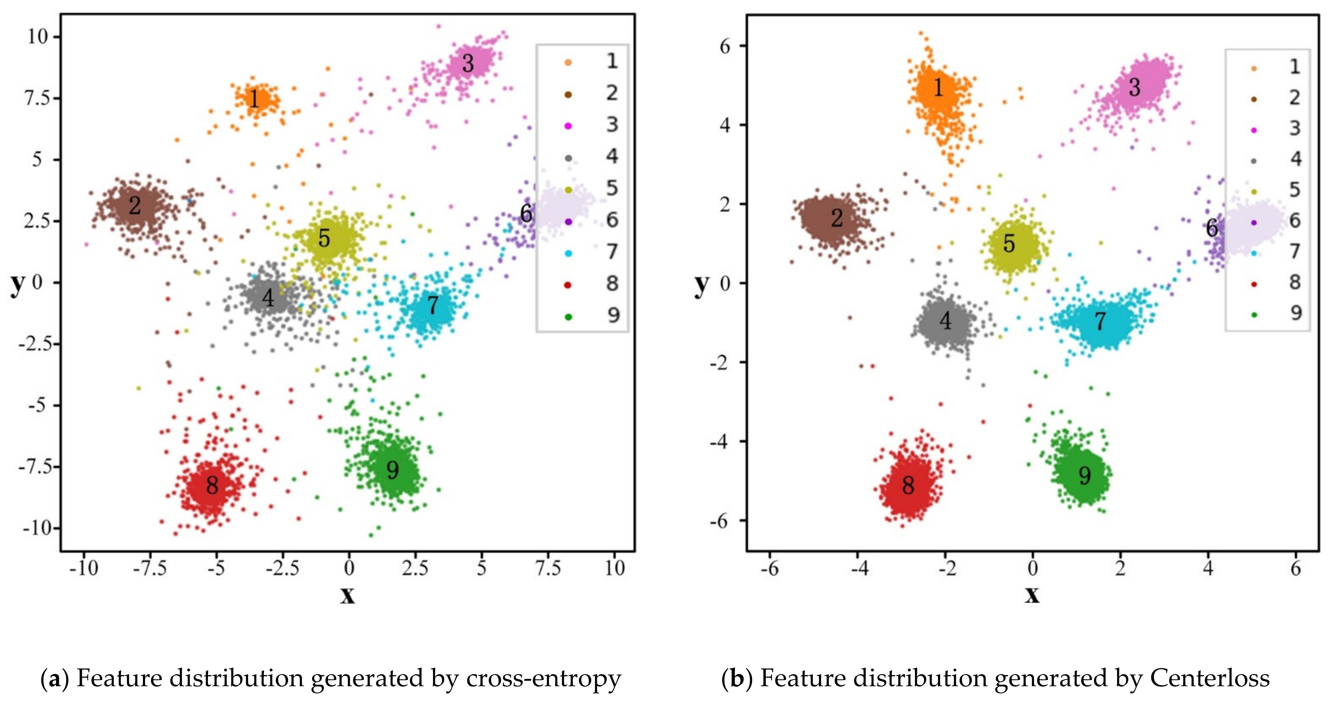
3.5. Improved Loss Function

Different categories of diseases may have very similar symptoms, which makes it hard for some disease characteristics extracted by the network to be accurately distinguished. Furthermore, in the practical work of crop leaf disease recognition, the features extracted by CNN should not only have separability, but also have a high discrimination degree, otherwise the generalization performance of models will be affected. One of the solutions to the above problem is to optimize loss function. The cross-entropy loss commonly adopted in CNN focuses more on the separability among target categories and ignores the problems existing within each category. This leads to the fact that although cross-entropy loss can maintain high performance in a closed data space, the recognition performance will be greatly reduced when facing unforeseen disease images. As a consequence, Centerloss [36] was introduced to aggregate each class of disease characteristics, so as to widen the inter-class distance and reduce the intra-class distance. Centerloss can be expressed by Equation (4).
L C = ε 2     i = 1 b   a i c k i   2 2
where ε is related to the recognizable extent of the extracted features, and ε is set to 0.01; b represents the number of samples in each batch; a i represents the feature extracted from the ith sample in the same batch; k represents the number of different categories and c k i represents the feature center of the category to which ith sample belongs. Thus, Equation (5) can be obtained by optimizing cross-entropy loss.
L = L C E + L C = L C E + ε 2     i = 1 b   a i c k i   2 2
where L C E is cross-entropy loss. When the sample features in batch are misclassified, that is, the gap between a i and c k i is larger and the values of L and L C will also increase. At this time, Equation (5) plays a role in increasing the inter-class distance. When correctly classified, Equation (5) is served to reduce the intra-class distance accordingly.

3.6. Experiments Setup

The parameters involved in the experiment are exhibited in Table 2. In order to prevent falling into local optimization, the attenuation coefficient of learning rate was set to 0.8; that is, after 10 epochs, the learning rate would decay to 80% of the original. All experiments were run on a Ubuntu 18.04 LTS 64-bit system environment. Pytorch 1.6 was adopted, which supports GPU acceleration and dynamic neural networks. Additionally, CUDA 9.1 was used to assist in training. The computer is equipped with 32GB RAM and NVIDIA GeForce GTX 2080Ti.

3.7. Evaluation Index

Due to the data samples are unbalanced, this study objectively evaluates the model from five aspects, i.e., Micro_sensitivity, Micro_precision, Micro_F1 score, balanced accuracy and accuracy. The specific calculation formula is shown in (6)–(10) [12]:
M i c r o _ S e n s i t i v i t y = i = 1 9 T P i i = 1 9 T P i + i = 1 9 F N i × 100 %
M i c r o _ P r e c i s i o n = i = 1 9 T P i i = 1 9 T P i + i = 1 9 F P i × 100 %
M i c r o _ F 1 = 2 × M i c r o _ S e n s i t i v i t y × M i c r o _ P r e c i s i o n M i c r o _ S e n s i t i v i t y + M i c r o _ P r e c i s i o n
B a l a n c e d   A c c u r a c y = T P R   +   T N R 2 W h e r e     T P R = T P T P   +   F N T N R = T N F P   +   T N
A c c u r a c y = T P + T N T P + T N + F P + F N
where i represents the the disease category. Dataset1 involves 9 kinds of diseases, so the value range of i is 1 to 9. TP indicates that the prediction is a positive example and the actual is a positive example; FP indicates that the prediction is positive and the actual is negative; TN indicates that the prediction is negative and the actual is negative; FN indicates that the prediction is negative and the actual is positive. Sensitivity represents the ratio of the number of correctly predicted positive samples to the total number of real positive samples; Precision represents the ratio of the number of correctly predicted positive samples to the number of all predicted positive samples; and F1 is the harmonic mean of Sensitivity and Precision. In this paper, the above formula is processed by micro average; that is, the corresponding average value is calculated according to the contribution degree of each type of sample. TPR is actually Sensitivity; TNR can be understood as how many of all negative classes are predicted to be negative; Balanced Accuracy is an index used to evaluate unevenly distributed data; and Accuracy refers to the ratio of the number of correctly predicted samples to the total number of samples.

4. Results and Discussion

Firstly, in order to level the playing field between the improved model and the models proposed in other articles, they were trained and tested separately on the same version of Plant Village. Secondly, ablation experiments were conducted on Dataset1 to verify the effectiveness of different improved methods. Thirdly, the results are compared with those of other 8 studies in Section 4.3. Finally, in Section 4.4, the generalization performance of the improved model was discussed by experimenting on Dataset2.

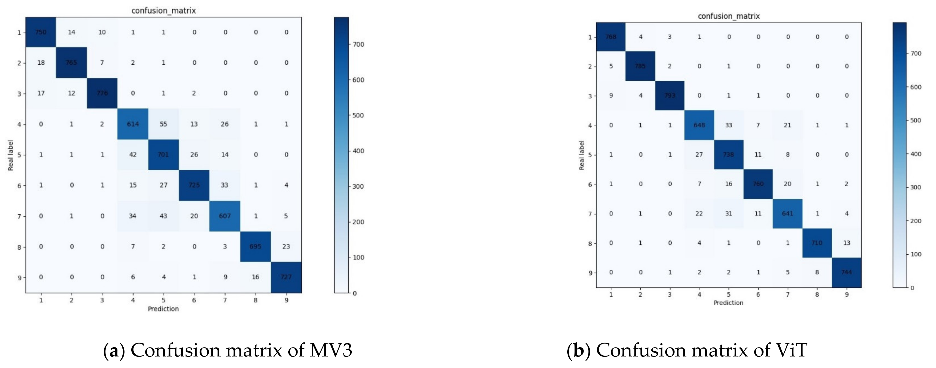
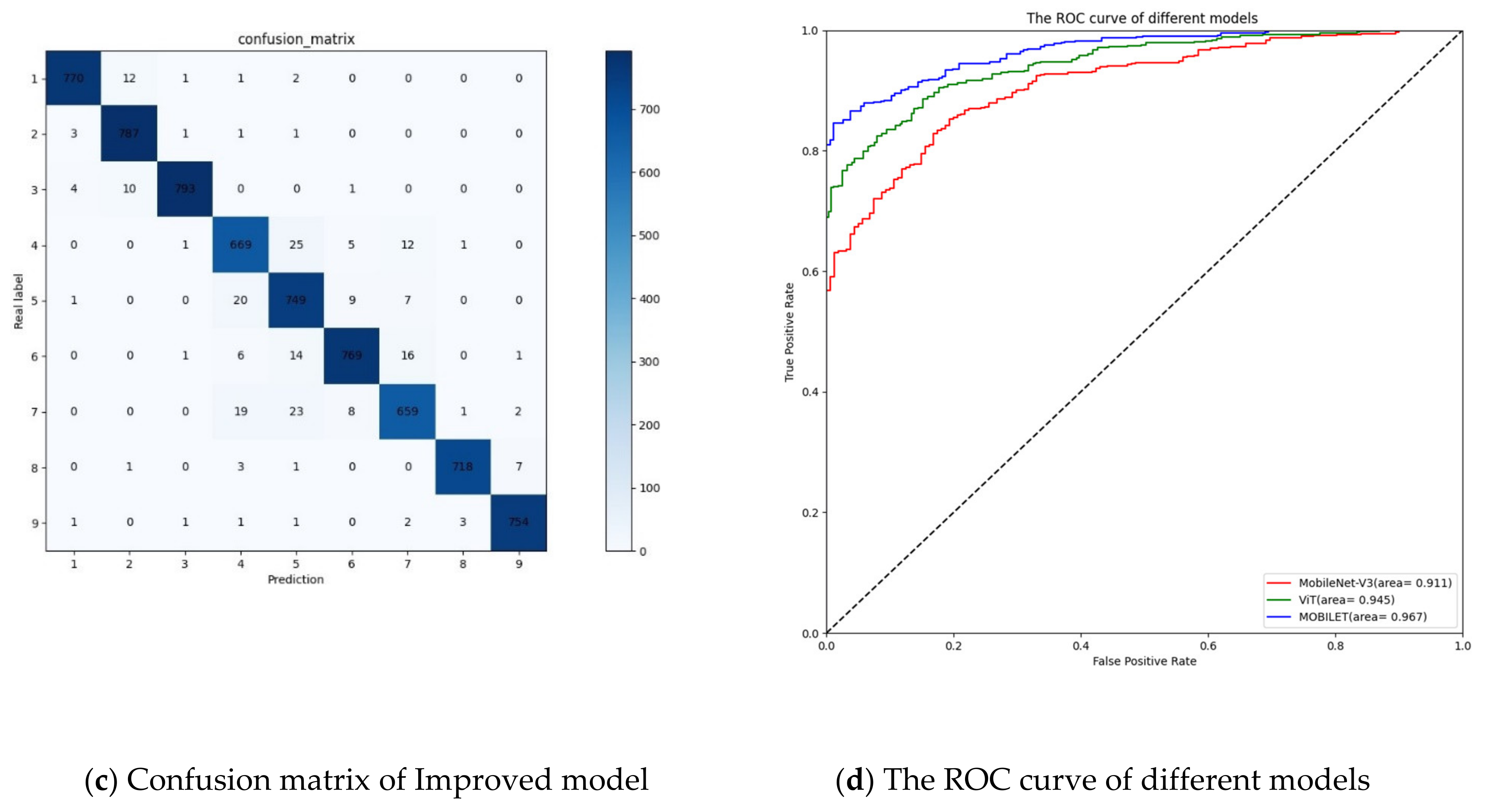
4.1. Results of Different Models on Plant Village

Mohameth et al. [15], Mohanty et al. [16] and Huang et al. [17] adopted the same version of Plant Village and their experimental results were highly comparable. During the pre-training, they saved the best weights obtained by their models, and after fine-tuning the weight parameters, they migrated them to Plant Village to complete the evaluation of improved models. The results obtained by the above methods are displayed in Table 3, where Mohameth et al. only evaluated the color version of Plant Village. In order to ensure the fairness of the experiment, three models were reconfigured according to the parameter settings in the articles, and we compared them with the improved model proposed to this study. Table 3 shows that the recognition accuracies on three versions of Plant Village achieved by improved model are 99.62%, 99.08%, and 99.22%, respectively, which was more competitive than the other methods. However, the composition of images in Plant Village is simple, which cannot provide further effective reference for the actual disease recognition. Consequently, in the subsequent part, the crop leaf disease images under complex backgrounds would be taken as the research object to explore and solve the difficulties faced by the disease recognition work in the field.

4.2. Ablation Study on Dataset1

The characteristics in ImageNet are diverse, which are redundant for work with only crop leaves, so we used Plant Village to pre-train the models. Moreover, a series of ablation experiments were conducted for the above improvement strategies, and the experimental results are shown in Table 4. On the basis of Plan0, Plan1 used Centerloss to optimize cross-entropy loss, and Balanced Acurracy, Micro_Sensitivity, Micro_Precision and Micro_F1 were improved by 1.65, 1.85, 2.11 and 1.99 percentage points, respectively, without increasing the number of parameters. Plan2 introduced Transformer on the basis of Plan0, which improved Balanced Acurracy, Micro_Sensitivity, Micro_Precision and Micro_F1 by 2.89, 3.52, 3.83, and 3.68 percentage points, respectively, while increasing the number of acceptable parameters. Compared with Plan1 and Plan2, the indicators of Plan3 have been further improved. In order to further analyze the advantages of the improved model, the more detailed and comprehensive comparative analyses of the above improved methods were carried out.
A kind of leaf disease may have multiple symptoms, one of which may be highly confused with the characteristics of other types of diseases in different periods. As illustrated in Figure 8, the initial stage of cassava bacterial blight shows symptoms including wet stain and white mucus, and in the later stage, the leaf color changes into yellowish brown, with withered and rotten leaves appearing. The late symptoms of cassava brown streak disease are similar to those of cassava bacterial blight, with tawny markings on the leaves and often accompanied by withered leaves. The symptoms of cassava leaf infected with mosaic virus are yellowing and curling, which are also very similar to the characteristics of the first two types of diseases, so it is difficult to distinguish them directly by the naked eye. The above situation will also result in misclassification of CNN models. The root of this problem is that different leaf diseases belonging to the same category have a highly similar color, shape and other characteristics, in brief, little differences in inter-class characteristics of diseases, but rich and large differences in intra-class characteristics. To address the above problem, Centerloss was used as a penalty term to optimize cross-entropy loss, and Figure 9 visualized the effect before and after optimization. As shown in Figure 9a, before optimization, the distribution of disease features extracted by CNN is sparse, and there is a serious intersection among samples of different categories, indicating that these samples are likely to be misclassified in the subsequent recognition work. As shown in Figure 9b, after optimization, features belonging to the same cluster converge towards the corresponding feature center, and the distance between different clusters is enlarged. The comparison results show that the introduction of Centerloss makes the originally scattered disease feature distribution more concentrated, and at the same time, the separability of similar disease features has been further expanded.
Plan 2 introduced Transformer Encoder into MobileNet-V2, which made CNN encode the global information and extract the local features of the disease images at the same time. In other words, Transformer Encoder was regarded as convolution operations to learn the global features of the disease images. The variation of balanced accuracy produced by different models using this strategy is shown in Figure 10. In addition, heat maps were applied to visualize the attention distribution of the models. In Figure 11 (red regions represent important features, and regions covered by other colors are considered as secondary features), the pure CNN models focus mostly on the edge area of leaves, which proves that the pure CNN models are really good at extracting local features of the images. However, it also exposes some problems, that is, compared with the whole leaf, the diseased area is generally small, and the pure CNN models are easy to focus attention on the textures, edges and other features of leaves. In contrast, CNN models, with Transformer Encoder, can focus more attention on the lesion regions. This phenomenon can be interpreted as the improved model with global and local feature information, which has acquired the stronger ability of feature extraction and generalization in several iterations of training. Furthermore, the performance of different CNN models using this improved strategy has been improved to a certain extent, which also confirms the importance of global features for leaf disease recognition.
In conclusion, the recognition situations of different models on each category of disease images are listed in Table 5. In terms of weighed accuracy, compared with the other two models, the improved model in this study shows certain advantages in recognizing each kind of diseases, with an accuracy of 96.58%, which is 1.27~4.56% higher than the other models.
Due to the introduction of Transformer Encoder, the improved model is slightly more than the lightweight MobileNet-V3 in terms of parameter quantity by 0.62 M. However, generally speaking, a good balance has been achieved between recognition accuracy and parameter quantity in the improved model and its cost performance is more superior. Additionally, in order to more intuitively show the situation of recognition of each kind of disease image, the confusion matrixes and ROC curves obtained by the three models on Dataset1 were provided. The numbers on the main diagonal represent the sample sizes that were predicted correctly, and the remaining positions are the sample sizes that were predicted incorrectly. Comparing these three confusion matrixes, it can be seen that: (1) Compared with the pure CNN structure and the pure Transformer structure, the hybrid model proposed by us effectively reduces the misclassification of samples; (2) As shown in Figure 12a,b, and as mentioned above, the characteristics of different cassava diseases are relatively similar, which leads to the four disease images often being mis-indentified as each other (e.g., cassava brown streak and cassava bacterial blight are often misidentified with each other). However, the improved model in this paper effectively alleviates this situation, which shows that the improved method proposed in this paper can extract and analyze subtle and similar features more effectively. In addition, the ROC curves of the three models obtained on Dataset1 also show that the improved model proposed in this paper has better performance.

4.3. Comparisons with Results from Other Paper

In order to make the comparison results more comparable, we selected eight scientific studies with apple, cassava and cotton as the experimental objects. It can be seen from Table 6 that, compared with the recognition accuracy obtained by the models in the other eight studies, the hybrid model proposed in this paper is at least 1.03%, 1.26% and 1.40% higher than the former in apple, cassava and cotton, respectively. This shows that the hybrid model based on CNN and Transformer proposed in this paper has a higher accuracy in recognizing diseases.

4.4. Generalization on Dataset2

The training and test sets in Section 4.2 were shot in the same environment, which have certain similarities and cannot be applied to verify the generalization performance of models. In other words, training data from the same source may result in poor generalization performance of the final model, which is detrimental for identifying crop diseases in different regions. In addition, an excellent model also needs to have mighty prediction ability when facing unforeseen data; hence, the test set in Section 4.2 was substituted by Dataset2 to inspect the generalization performance of the improved model. As shown in Table 7, affected by backgrounds replacement, the recognition accuracies of various models decreased to a certain extent. However, the improved model in this study still achieved the highest recognition accuracy, which showed that the improved model has better generalization ability when facing unforeseen data and can better meet the requirements of field disease recognition.

5. Conclusions

Based on the tasks of field crop disease recognition, the datasets used in this study were closer to the production needs in real life. In response to the characteristics of crop disease features in complex environment, which includes wide distribution regions and irregular distribution, we analyzed the shortcomings of MobileNet-V2 and made the improved model achieve a good balance between recognition accuracy and parameter quantity. The attention of the improved model was more focused on the diseased regions by introducing Transformer Encoder, which also improved the ability of extracting global disease features. Based on cross-entropy loss, Centerloss was introduced, which not only improved the separability of different disease features, but also made the sample features automatically cluster toward the feature center of the category they belong to. The recognition accuracy of 99.62% was achieved by the improved model on Plant Village. Even when facing the interference from complex backgrounds in Dataset1, the accuracy was higher than other models, reaching 96.58%. In Dataset2, the improved model proposed in this paper achieved recognition accuracy of 95.97%, 94.03% and 96.39%, respectively, which shows that the improved model has good generalization ability. Meanwhile, the improved model also has better recognition performance and less parameter quantity when compared with other superior models. In summary, the improved model in this study can better recognize crop leaf diseases under complex backgrounds, and provides ideas for transferring deep learning models to mobile disease detection devices.
At present, most of the mainstream crop disease identification methods study the diseased leaves, but early disease identification is more meaningful and more difficult. In the early stage of the disease, the disease spots are smaller and difficult to observe with the naked eye. Before the disease spots are formed, the image identification method based on RGB cannot recognize this kind of disease images. Therefore, in the follow-up work, the multimodal images of crop diseases can be introduced into deep learning, and the multimodal images can be fused to realize the early identification of diseases.

Author Contributions

J.S. (Jun Sun) and W.Z. contributed to the development of the systems, including farm site data collection and the manuscript writing. W.Z. provided significant suggestions on the development and contributed to performance evaluation. S.W. and K.Y. contributed to grammar modification. J.S. (Jifeng Shen), X.Z., S.W. and K.Y. analyzed the results. All authors wrote the manuscript together. All authors have read and agreed to the published version of the manuscript.

Funding

This work is partly supported by Project of Faculty of Agricultural Equipment of Jiangsu University (NZXB20210210), a project funded by the Priority Academic Program Development of Jiangsu Higher Education Institutions (PAPD), and Jiangsu University undergraduate scientific research project (20AB00).

Institutional Review Board Statement

Not applicable.

Informed Consent Statement

Not applicable.

Data Availability Statement

The data used and/or analyzed during the current study are available from the corresponding author on reasonable request.

Conflicts of Interest

The authors declare no conflict of interest.

References

  1. Gu, Y.H.; Yin, H.; Jin, D.; Zheng, R.; Yoo, S.J. Improved multi-plant disease recognition method using deep convolutional neural networks in six diseases of apples and pears. Agriculture 2022, 12, 300. [Google Scholar] [CrossRef]
  2. Wagle, S.A.; Harikrishnan, R.; Ali, S.H.M.; Faseehuddin, M. Classification of plant leaves using new compact convolutional neural network models. Plants 2022, 11, 24. [Google Scholar] [CrossRef] [PubMed]
  3. Nasirahmadi, A.; Wilczek, U.; Hensel, O. Sugar beet damage detection during harvesting using different convolutional neural network models. Agriculture 2021, 11, 1111. [Google Scholar] [CrossRef]
  4. Sun, J.; He, X.F.; Tan, W.J.; Wu, X.H.; Lu, H. Recognition of crop seedling and weed recognition based on dilated convolution and global pooling in CNN. Trans. Chin. Soc. Agric. Eng. 2018, 34, 159–165. [Google Scholar] [CrossRef]
  5. Machado, B.B.; Orue, J.P.M.; Arruda, M.S.; Santos, C.V.; Sarath, D.S.; Goncalves, W.N. Bioleaf: A professional mobile application to measure foliar damage caused by insect herbivory. Comput. Electron. Agric. 2016, 129, 44–55. [Google Scholar] [CrossRef] [Green Version]
  6. Xu, P.; Tan, Q.; Zhang, Y.; Zha, X.; Yang, S.; Yang, R. Research on maize seed classification and recognition based on machine vision and deep learning. Agriculture 2022, 12, 232. [Google Scholar] [CrossRef]
  7. Sun, J.; He, X.; Ge, X.; Wu, X.; Shen, J.; Song, Y. Detection of key organs in tomato based on deep migration learning in a complex background. Agriculture 2018, 8, 196. [Google Scholar] [CrossRef] [Green Version]
  8. Luo, H.; Dai, S.; Li, M.; Liu, E.P.; Zheng, Q.; Hu, Y.; Yi, X.P. Comparison of machine learning algorithms for mapping mango plantations based on Gaofen-1 imagery. J. Integr. Agric. 2020, 19, 2815–2828. [Google Scholar] [CrossRef]
  9. Ashwinkumar, S.; Rajagopal, S.; Manimaran, V.; Jegajothi, B. Automated plant leaf disease detection and classification using optimal MobileNet based convolutional neural networks. Mater. Today Proc. 2021, 51, 480–487. [Google Scholar] [CrossRef]
  10. Kamal, K.C.; Yin, Z.; Wu, M.; Wu, Z.L. Depthwise separable convolution architectures for plant disease classification. Comput. Electron. Agric. 2019, 165, 104948. [Google Scholar] [CrossRef]
  11. Ji, M.; Zhang, L.; Wu, Q. Automatic grape leaf diseases identification via united model based on multiple convolutional neural networks. Inf. Process. Agric. 2020, 7, 418–426. [Google Scholar] [CrossRef]
  12. Sun, J.; Tan, W.; Mao, H.P.; Wu, X.H.; Chen, Y.; Wang, L. Recognition of multiple plant leaf diseases based on improved convolutional neural network. Trans. Chin. Soc. Agric. Eng. 2017, 33, 209–215. [Google Scholar] [CrossRef]
  13. Too, E.C.; Li, Y.J.; Njuki, S.; Liu, Y.C. A comparative study of fine-tuning deep learning models for plant disease identification. Comput. Electron. Agric. 2019, 161, 272–279. [Google Scholar] [CrossRef]
  14. Zhao, L.X.; Hou, F.D.; Lu, L.Z.; Zhu, H.C.; Ding, X.L. Image recognition of cotton leaf diseases and pests based on transfer learning. Trans. Chin. Soc. Agric. Eng. 2020, 36, 184–191. [Google Scholar] [CrossRef]
  15. Mohameth, F.; Chen, B.C.; Kane, A.S. Plant disease detection with deep learning and feature extraction using plant village. J. Computer. Commun. 2020, 8, 10–22. [Google Scholar] [CrossRef]
  16. Mohanty, S.P.; Hughes, D.P.; Salathe, M. Using deep learning for image-based plant disease detection. Front. Plant. Sci. 2016, 7, 159–167. [Google Scholar] [CrossRef] [Green Version]
  17. Huang, J.P.; Chen, J.; Li, K.X.; Li, J.Y.; Liu, H. Identification of multiple plant leaf diseases using neural architecture search. Trans. Chin. Soc. Agric. Eng. 2020, 36, 166–173. [Google Scholar] [CrossRef]
  18. Gao, R.; Wang, R.; Feng, L.; Li, Q.; Wu, H.R. Dual-branch, efficient, channel attention-based crop disease identification. Comput. Electron. Agric. 2021, 190, 106410. [Google Scholar] [CrossRef]
  19. Zhou, J.; Li, J.X.; Wang, C.S.; Wu, H.R.; Zhao, C.J.; Teng, G.F. Crop disease identification and interpretation method based on multimodal deep learning. Comput. Electron. Agric. 2021, 189, 106408. [Google Scholar] [CrossRef]
  20. Picon, A.; Seitz, M.; Alvarez, G.A.; Mohnke, P.; Ortiz, B.A.; Echazarra, J. Crop conditional convolutional neural networks for massive multi-crop plant disease classification over cell phone acquired images taken on real field conditions. Comput. Electron. Agric. 2019, 167, 105093. [Google Scholar] [CrossRef]
  21. Chen, J.; Zhang, D.; Suzauddola, M.; Zeb, A. Identifying crop diseases using attention embedded MobileNet-V2 model. Appl. Soft Comput. 2021, 113, 107901. [Google Scholar] [CrossRef]
  22. Wang, C.S.; Zhou, J.; Wu, H.R.; Teng, G.F.; Zhao, C.J.; Li, J.X. Identification of vegetable leaf diseases based on improved multi-scale ResNet. Trans. Chin. Soc. Agric. Eng. 2020, 36, 209–217. [Google Scholar] [CrossRef]
  23. Tang, Z.; Yang, J.L.; Li, Z.; Qi, F. Grape disease image classification based on lightweight convolution neural networks and channelwise attention. Comput. Electron. Agric. 2020, 178, 105735. [Google Scholar] [CrossRef]
  24. Machado, B.B.; Spadon, G.; Arruda, M.S.; Gon, W.N. A smartphone application to measure the quality of pest control spraying machines via image analysis. In Proceedings of the 33rd Annual ACM Symposium on Applied Computing, Pau, France, 9–13 April 2018; pp. 956–963. [Google Scholar] [CrossRef] [Green Version]
  25. Devlin, J.; Chang, M.W.; Lee, K.; Toutanova, K. Bert: Pre-training of deep bidirectional transformers for language understanding. In Proceedings of the 2019 Conference of the North American Chapter of the Association for Computational Linguistics: Human Language Technologies, Minneapolis, MN, USA, 2–7 June 2019; pp. 4171–4186. [Google Scholar] [CrossRef]
  26. Spadon, G.; Hong, S.; Brandoli, B.; Matwin, S.; Rodrigues, J.F., Jr.; Sun, J. Pay attention to evolution: Time series forecasting with deep graph-evolution learning. arXiv 2008, arXiv:2008.12833v3. [Google Scholar] [CrossRef]
  27. Hossain, S.; Deb, K.; Dhar, P.; Koshiba, T. Plant leaf disease recognition using depth-wise separable convolution-based models. Symmetry 2021, 13, 511. [Google Scholar] [CrossRef]
  28. Dataset1. Available online: https://www.kaggle.com (accessed on 20 October 2021).
  29. Wagle, S.A.; Harikrishnan, R. A deep learning-based approach in classification and validation of tomato leaf disease. Trait. Signal 2021, 38, 699–709. [Google Scholar] [CrossRef]
  30. Wagle, S.A.; Harikrishnan, R.; Sampe, J.; Mohammad, F.; Md Ali, S.H. Effect of data augmentation in the classification and validation of tomato plant disease with deep learning methods. Trait. Signal 2021, 38, 1657–1670. [Google Scholar] [CrossRef]
  31. Bruno, B.; Gabriel, S.; Travis, E.; Patrick, H.; Andre, C. Dropleaf: A precision farming smartphone tool for real-time quantification of pesticide application coverage. Comput. Electron. Agric. 2021, 180, 105906. [Google Scholar] [CrossRef]
  32. Castro, A.D.; Madalozzo, G.A.; Trentin, N.; Costa, R.; Rieder, R. Berryip embedded: An embedded vision system for strawberry crop. Comput. Electron. Agric. 2020, 173, 105354. [Google Scholar] [CrossRef]
  33. Yadav, S.; Sengar, N.; Singh, A.; Singh, A.; Dutta, M.K. Identification of disease using deep learning and evaluation of bacteriosis in peach leaf. Ecol. Inform. 2021, 61, 101247. [Google Scholar] [CrossRef]
  34. Sandler, M.; Howard, A.; Zhu, M.; Zhmoginov, A.; Chen, L.C. MobileNetV2: Inverted residuals and linear bottlenecks. In Proceedings of the IEEE Conference on Computer Vision and Pattern Recognition (CVPR2018), Salt Lake City, UT, USA, 18–22 June 2018; pp. 4510–4520. [Google Scholar]
  35. Vaswani, A.; Shazeer, N.; Parmar, N.; Uszkoreit, J.; Jones, L.; Gomez, A.N.; Kaiser, L.; Polosukhin, I. Attention is all you need. In Proceedings of the Advances in Neural Information Processing Systems (NIPS2017), Long Beach, CA, USA, 4–9 December 2017; pp. 5998–6008. [Google Scholar]
  36. Wen, Y.; Zhang, K.; Li, Z.; Yu, Q. A discriminative feature learning approach for deep face recognition. In Proceedings of the European Conference on Computer Vision (ECCV2016), Amsterdam, The Netherlands, 11–14 October 2016; pp. 499–515. [Google Scholar] [CrossRef]
  37. Luo, Y.Q.; Sun, J.; Shen, J.F.; Wu, X.H.; Wang, L.; Zhu, W.D. Apple leaf disease recognition and sub-class categorization based on improved multi-scale feature fusion network. IEEE Access 2021, 9, 95517–95527. [Google Scholar] [CrossRef]
  38. Sun, J.; Zhu, W.D.; Luo, Y.Q. Recognizing the diseases of crop leaves in fields using improved Mobilenet-V2. Trans. Chin. Soc. Agric. Eng. 2021, 37, 161–169. [Google Scholar] [CrossRef]
  39. Liu, Y.; Gao, G.Q. Identification of multiple leaf diseases using improved SqueezeNet model. Trans. Chin. Soc. Agric. Eng. 2021, 37, 187–195. [Google Scholar] [CrossRef]
  40. Yadav, D.; Akanksha; Yadav, A.K. A novel convolutional neural network-based model for recognition and classification of apple leaf diseases. Trait. Signal 2020, 37, 1093–1101. [Google Scholar] [CrossRef]
  41. Ramcharan, A.; McCloskey, P.; Baranowski, K.; Mbilinyi, N.; Mrisho, L. A mobile-based deep learning model for cassava disease diagnosis. Front. Plant Sci. 2019, 10, 272. [Google Scholar] [CrossRef] [Green Version]
  42. Sambasivam, G.; Opiyo, G.D. A predictive machine learning application in agriculture: Cassava disease detection and classification with imbalanced dataset using convolutional neural networks. Egypt. Inform. J. 2021, 22, 27–34. [Google Scholar] [CrossRef]
  43. Caldeira, R.F.; Santiago, W.E.; Teruel, B. Identification of cotton leaf lesions using deep learning techniques. Sensors 2021, 21, 3169. [Google Scholar] [CrossRef]
Figure 1. Leaf disease images with simple background in Plant Village.
Agriculture 12 01083 g001
Figure 2. Leaf disease images in natural scene.
Agriculture 12 01083 g002
Figure 3. Number of images before and after augmentation, where 1~9 in the X axis represent Apple—healthy, rust, scab; Cassava—bacterial blight, brown streak, healthy, mosaic virus; Cotton boll—blight, healthy.
Agriculture 12 01083 g003
Figure 4. The process of background replacement.
Agriculture 12 01083 g004
Figure 5. Structure of MobileNet-V2. The parameters next to the silver-gray downward arrow represent the number and stride of convolution kernels. BN represents Inverted Residual Block. DWConv is Depthwise Convolution, which is an important part of depthwise separable convolution.
Agriculture 12 01083 g005
Figure 6. Structure of Transformer Encoder. The right side of the dashed line indicates that the linear transformation of In(x) is equally partitioned into h parts according to the number of groups. Attention map is obtained by matrix multiplication and Softmax, which is finally embedded in N(x) to obtain the global representation.
Agriculture 12 01083 g006
Figure 7. Hybrid model of CNN and Transformer. s represents stride, 2× means repeat twice, MT block is the abbreviation of Mobile-Transformer block, which represents the combination of CNN and Transformer and BN represents the Inverted Residual Block in MobileNet-V2. In MT module, the feature map of H × W is divided into B patches, then B patches are expanded and sent to the layer composed of R Transformer Encoder in series. Finally, the output of Transformer Encoder is folded and the attention embedding and feature fusion are completed.
Agriculture 12 01083 g007
Figure 8. Comparisons of symptoms of different diseased cassava leaves at different stages. cbb, cbs and cmv are the abbreviations of cassava bacterial blight, cassava brown streak, and cassava mosaic virus.
Agriculture 12 01083 g008
Figure 9. Visualization of characteristic distribution of various diseases. The abscissa and ordinate represent the distance between sample points, where 1:9 in the confusion matrix represents Apple—healthy, rust, scab; Cassava—bacterial blight, brown streak, healthy, mosaic virus; Cotton boll—blight, healthy.
Agriculture 12 01083 g009
Figure 10. The variation of balanced accuracy of different models after introducing Transformer Encoder. TL means transfer learning. TE represents Transformer Encoder.
Agriculture 12 01083 g010
Figure 11. Visual analysis of regions of interest of different models.
Agriculture 12 01083 g011
Figure 12. Confusion matrix and ROC curve obtained on Dataset1, where 1:9 in the confusion matrix represents Apple—healthy, rust, scab; Cassava—bacterial blight, brown streak, healthy, mosaic virus; Cotton boll—blight, healthy.
Agriculture 12 01083 g012aAgriculture 12 01083 g012b
Table 1. Comparative analysis of the related work on plant disease identification.
Ref No.ModelData SituationBackgroundAccuracyChallenges/Future Scope
[9]MobileNetFive tomato diseases in Plant VillageSimple98.50%The background of tomato disease is simple, and the images need a lot of complex preprocessing.
[10]MobileNetPlant VillageSimple98.34%The improved model has low recognition accuracy in the face of diseases in complex environment.
[11]Inception-V3 and ResNet-50Four grape diseases in Plant VillageSimple98.57%The background is simple, and the correlation between disease characteristics is not considered.
[17]NASPlant VillageSimple95.40%The improved model performs poorly on datasets with unbalanced quantity and requires a certain amount of operation time.
[18]ResNet-18Self-collected cucumber diseasesComplex98.54%The improved model ignores the relationship between cucumber disease characteristics and only pays attention to the separability between classes.
[20]ResNet-50Self-collected diseasesComplex98.00%The local limitations of the features extracted by CNN are not considered, which is not conducive to the early detection of the disease.
[21]MobileNet-V2Self-collected diseasesComplex99.13%The influence of unbalanced sample size on experimental results is not considered.
[22]ResNet-18Self-collected diseasesComplex93.05%The recognition accuracy is not high in complex background. Furthermore, the parameters of the model are large, and the image processing rate is not discussed.
[23]ShuffleNetFour grape diseasesComplex99.14%The influence of unbalanced data volume on experimental results is not considered, and how to expand intra class differences is not analyzed.
Table 2. Parameters and values adopted in the experiments.
ParametersValues
Classes on Dataset19
Classes on Dataset23
Image size256 × 256
Batch size32
Epochs150
Learning rate (LR)0.001
LR decay index80%
Dropout0.2
OptimizerAdam
β 1 , β 2 Default (0.9, 0.999)
Table 3. Comparisons of recognition accuracy of different models on three versions of Plant Village. The methods with prefix @ have been reconfigured. MV2 is the abbreviation of MobileNet-V2.
PaperBackoneTransfer LearningImage
Number
Accuracy (%)
ColorGraySegmented
Mohameth et al. [15]VGG1654,30697.82--
Mohanty et al. [16]AlexNet54,30699.2797.2698.91
Huang et al. [17]NasNet54,30698.9699.0195.40
@Mohameth et al. [15]VGG1654,30698.1497.6498.31
@Mohanty et al. [16]AlexNet54,30699.3697.9198.92
@Huang et al. [17]NasNet54,30699.1598.9698.66
This paperMV254,30699.6299.0899.22
Table 4. The results of ablation studies on Dataset1. The Plan column represents the different experimental models in the ablation experiment. Plan 0 represents the basic model MobileNet-V2. TL stands for transfer learning. Param represents parameter quantity. ‘-’ indicates that this improvement is not added; ‘√’ indicates adding this improvement.
PlanTLCenterlossTransformerBalanced
Accuracy (%)
Micro_
Sensitivity (%)
Micro_
Precision (%)
Micro_
F1 (%)
Param (M)
0--91.9491.6491.3791.502.24
1-93.5993.4993.4893.492.24
2-94.8295.1695.2095.185.00
396.5896.9796.7696.865.00
Table 5. Performance of different models on various disease images. MV3 is the abbreviation of MobileNet-V3, ViT is a pure Transformer model, MOBILET is the improved model proposed in this paper.
Crop NameDisease SituationAccuracy (%)
MV3ViTMOBILET
AppleHealthy96.7999.0299.37
Rust96.5099.0399.21
Scab96.0898.1198.90
CassavaBacterial blight86.1290.8993.76
Brown streak89.2893.9695.33
Mosaic virus85.3790.1792.66
Healthy89.8394.1595.30
CottonBoll blight95.1397.2898.34
Healthy95.2797.5198.77
Weighed accuracy (%)92.3195.6096.87
Param quantity (M)4.38103.035.00
Recognition speed per image (ms)4.248.774.93
Table 6. Comparisons with results from other papers.
PaperYearBackoneDatasetNumber of CategoriesAccuracy (%)
Zhao et al. [14]2020VGG-19Cotton697.16
Luo et al. [37]2021ResNet-50Apple694.99
Sun et al. [38]2021MobileNet-V2Cassava592.20
Liu et al. [39]2021SqueezeNetApple498.13
Yadav et al. [40]2020AlexNetApple498.00
Ramcharan et al. [41]2019MobileNetCassava383.90
Sambasivam et al. [42]2021Private modelCassava493.00
Caldeira et al. [43]2021GoogleNetCotton386.60
ResNet-50Cotton389.20
This paper2022MobileNet-V2 + TransformerCotton298.56
Apple399.16
Cassava494.26
Table 7. Differences in generalization ability among different models.
ModelAccuracy in Simple Background (%)Accuracy with Background Replacement (%)
Apple ScabCassava Brown StreakCotton Boll BlightApple ScabCASSAVA Brown StreakCotton Boll Blight
MV395.1493.3395.9792.2291.1193.47
ViT97.2293.8997.6493.8991.5394.72
MOBILET98.3395.4298.8995.9794.0396.39
Publisher’s Note: MDPI stays neutral with regard to jurisdictional claims in published maps and institutional affiliations.

