
Trends Analysis of Simultaneously Extracted Metal Copper Sediment Concentrations from a California Agricultural Waterbody including Historical Comparisons with Other Agricultural Waterbodies

Abstract
:1. Introduction
2. Materials and Methods
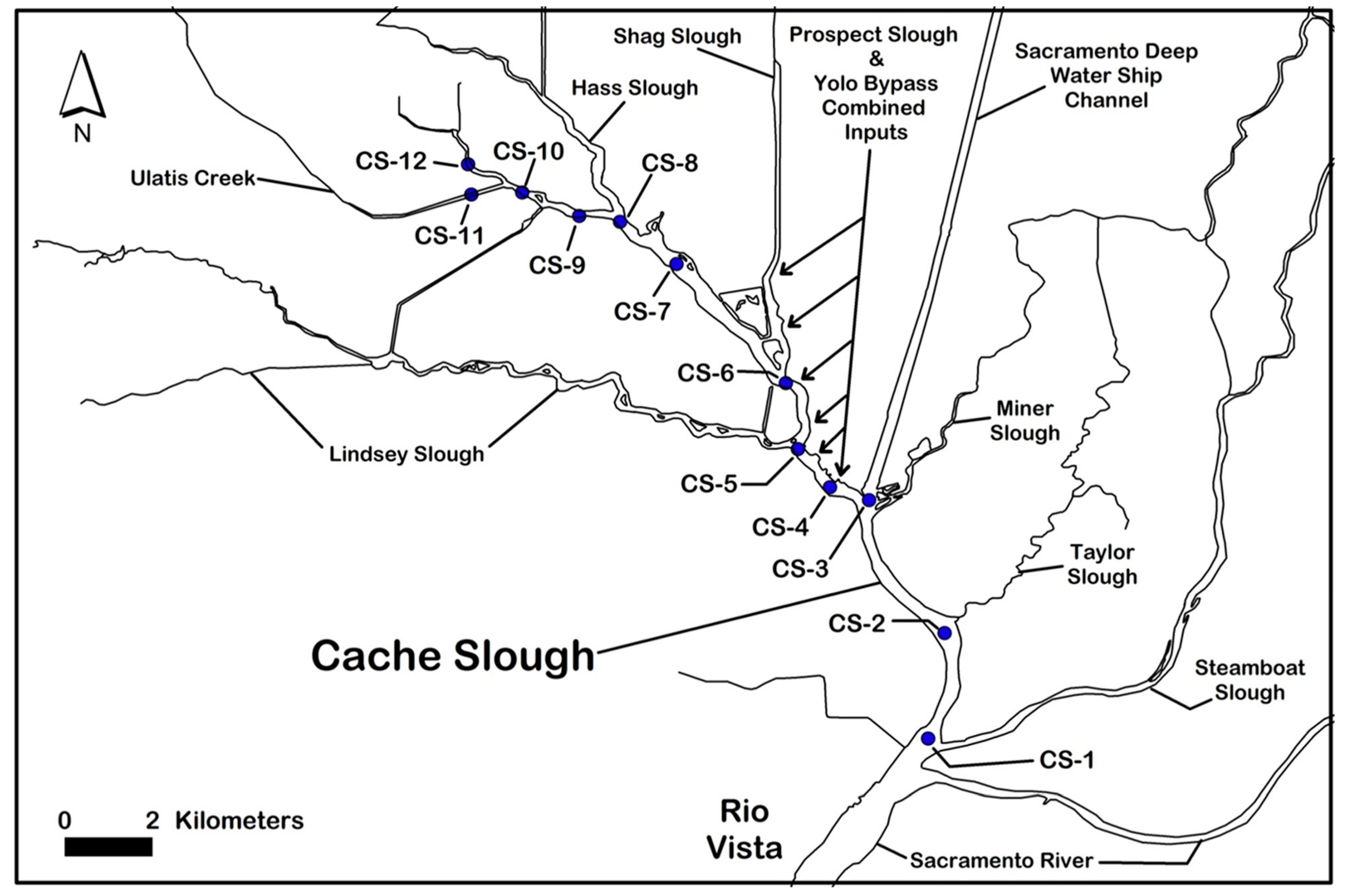
2.1. Sites Sampled and Collection Methods
2.2. SEM Copper Analysis
2.3. Statistical Analysis
3. Results
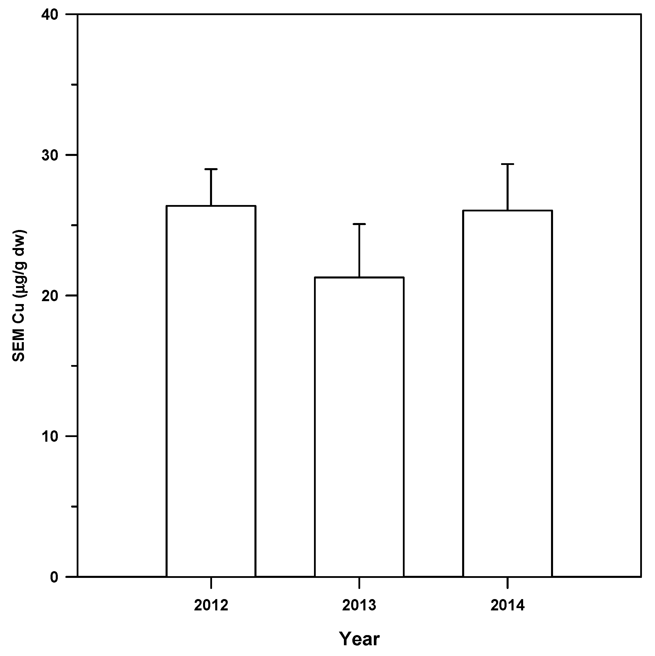
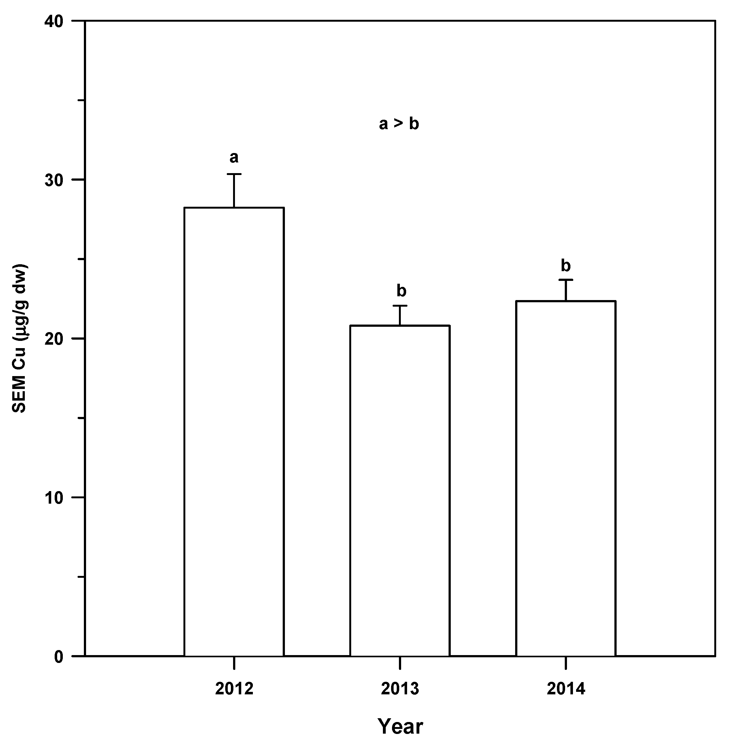
3.1. Summary Statistics
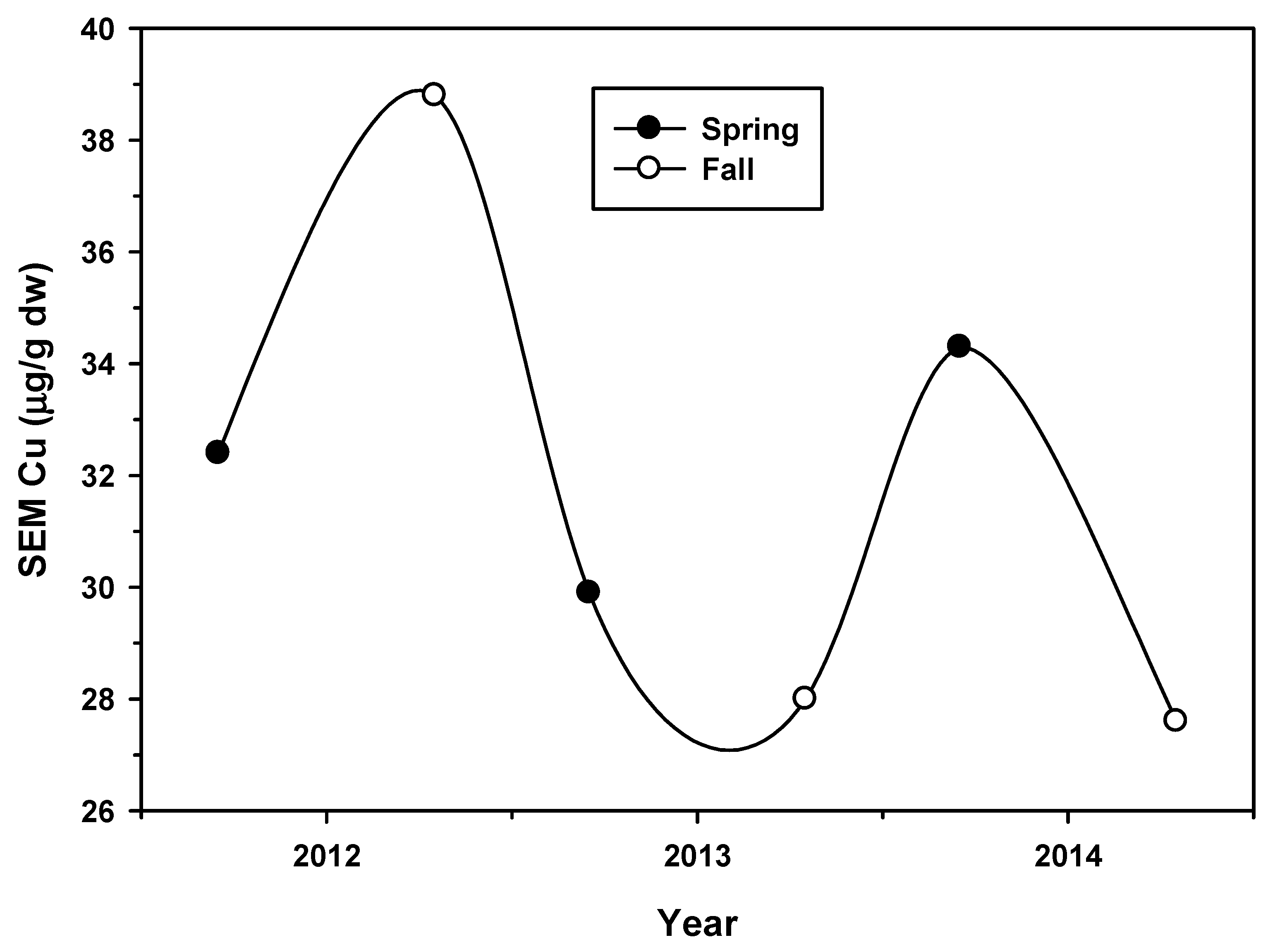
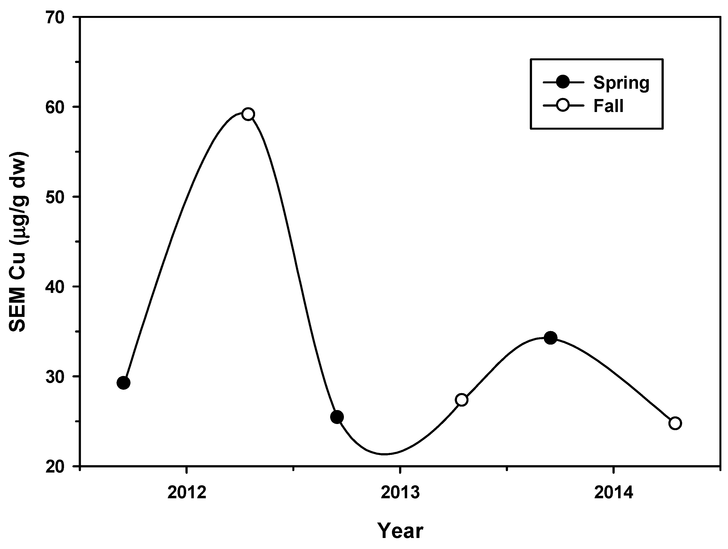
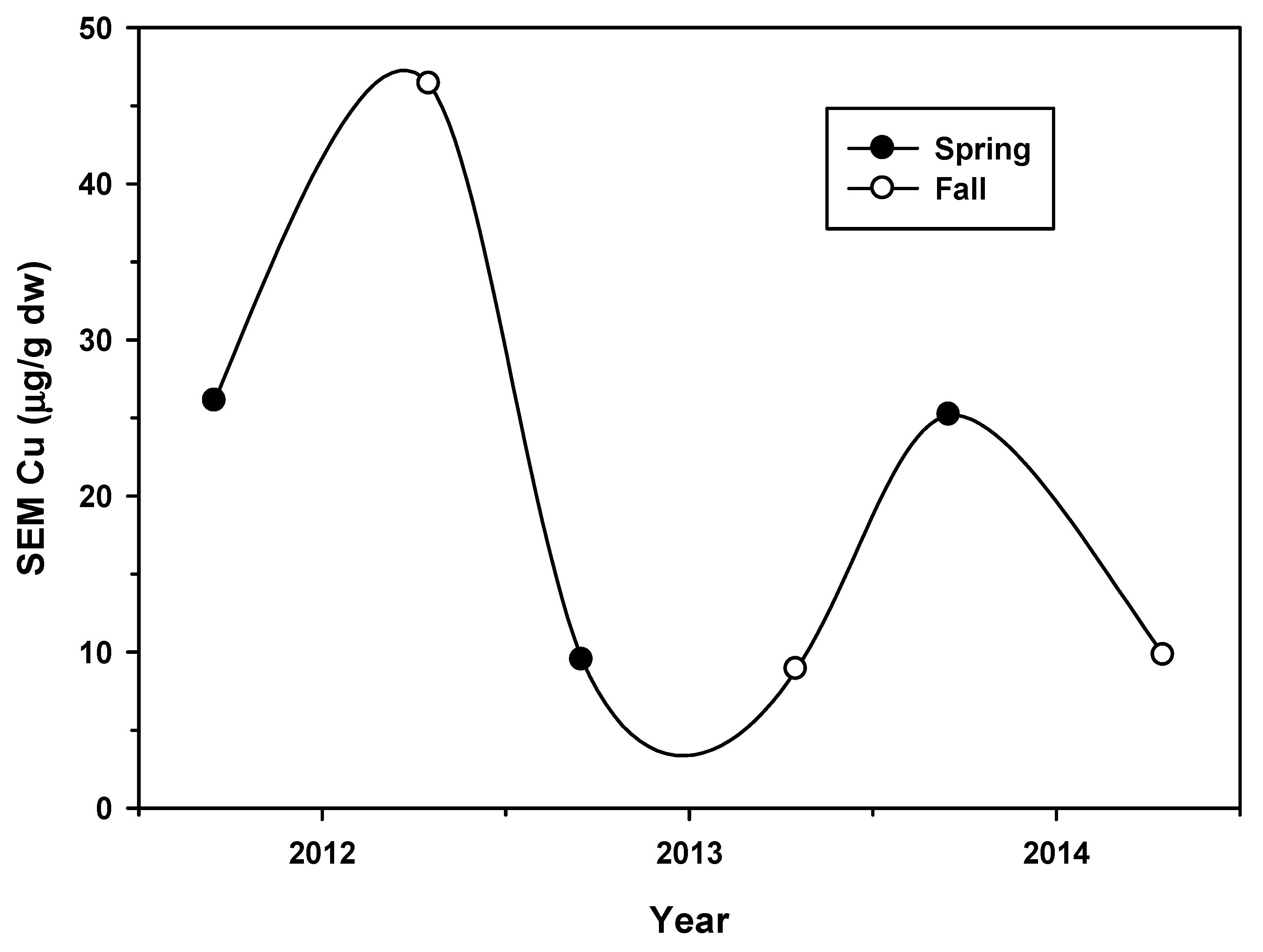
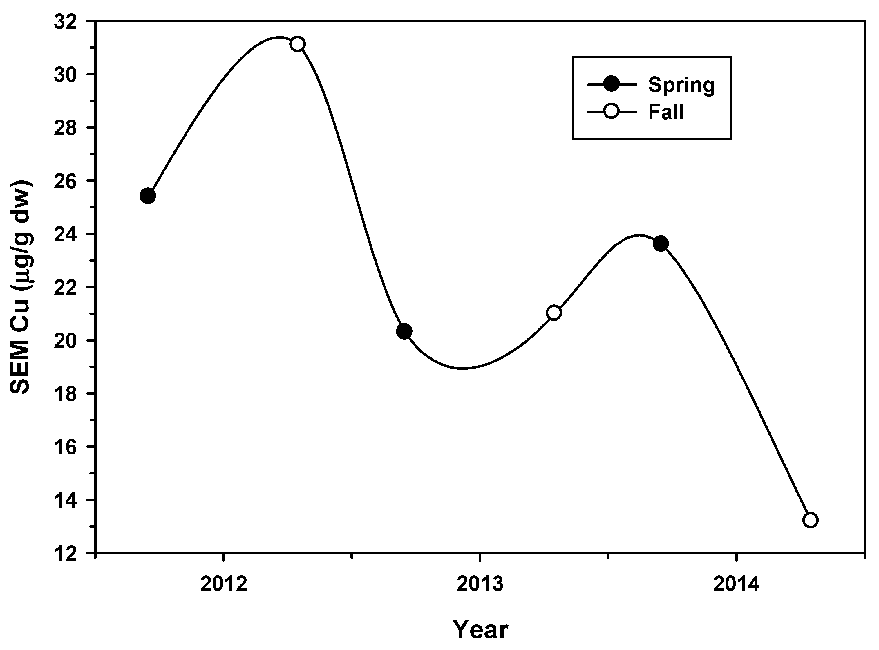
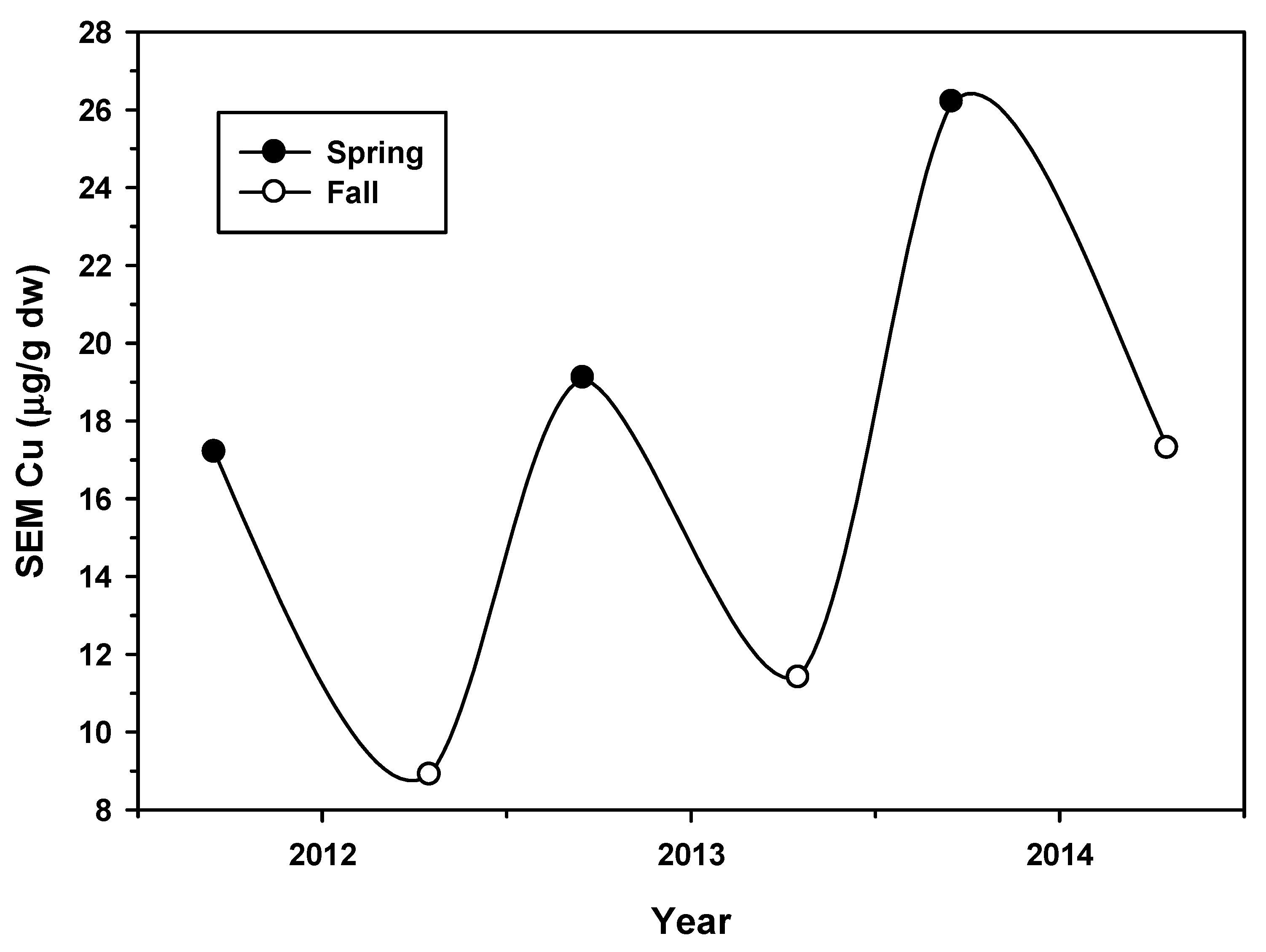
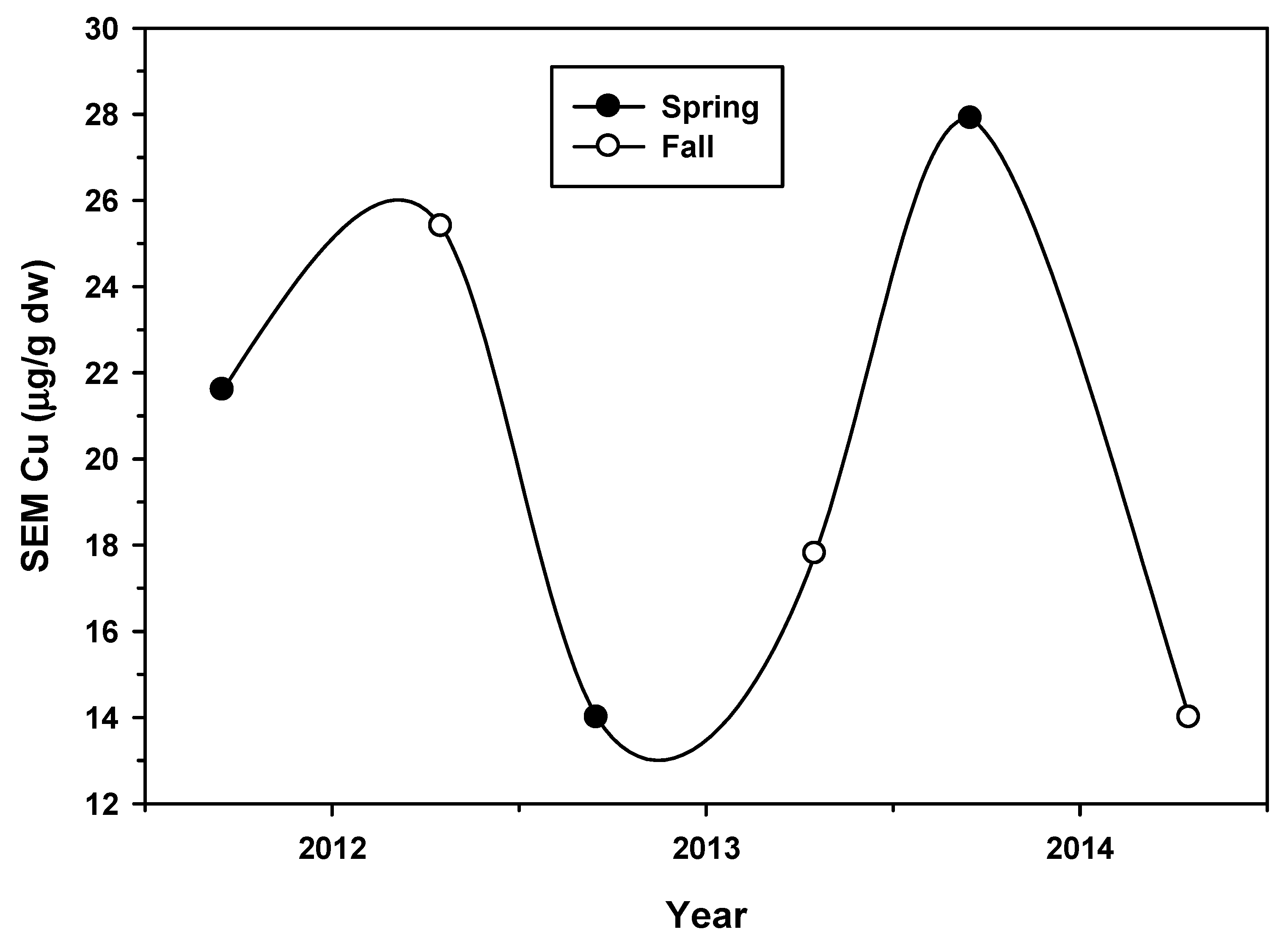
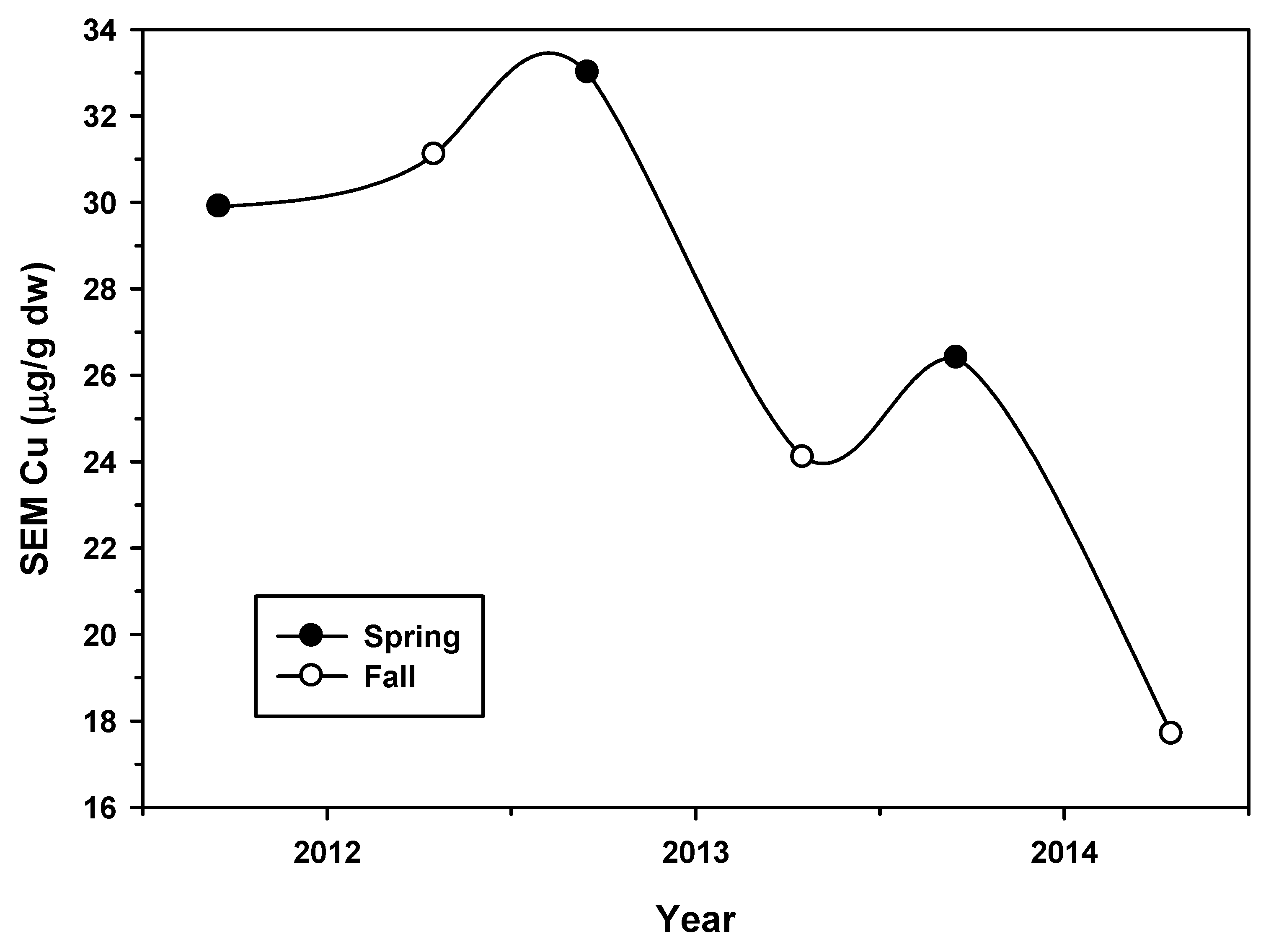
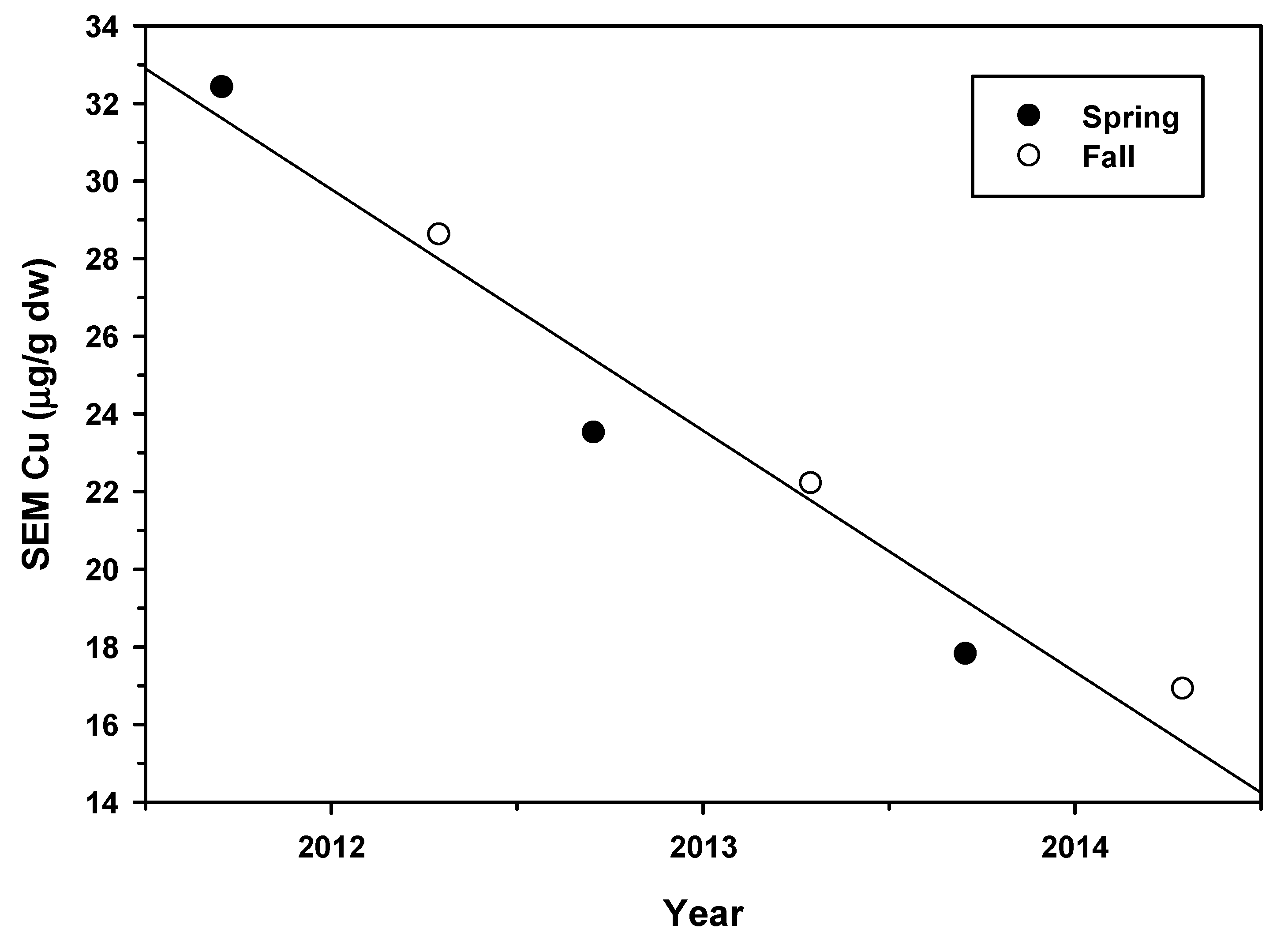
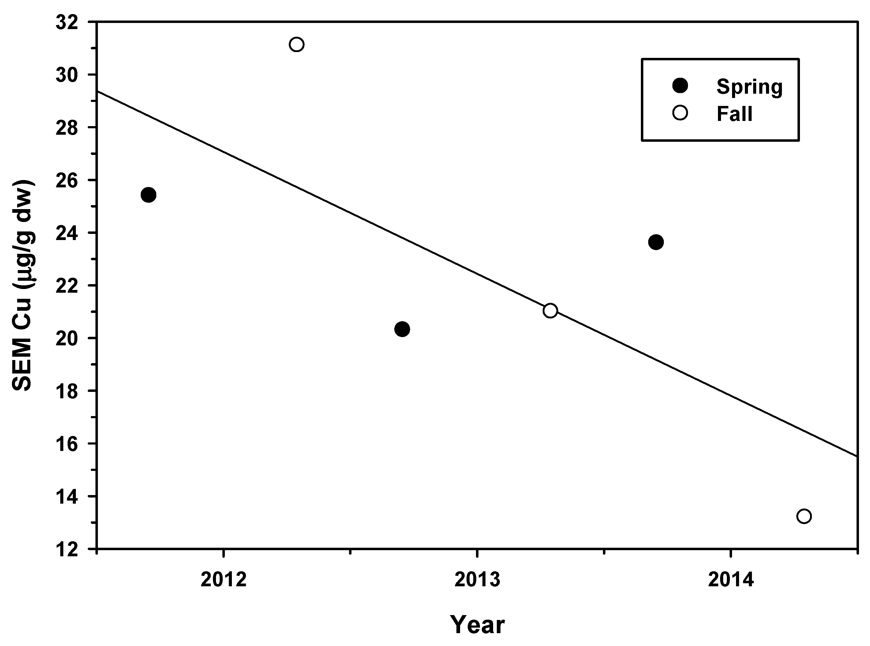
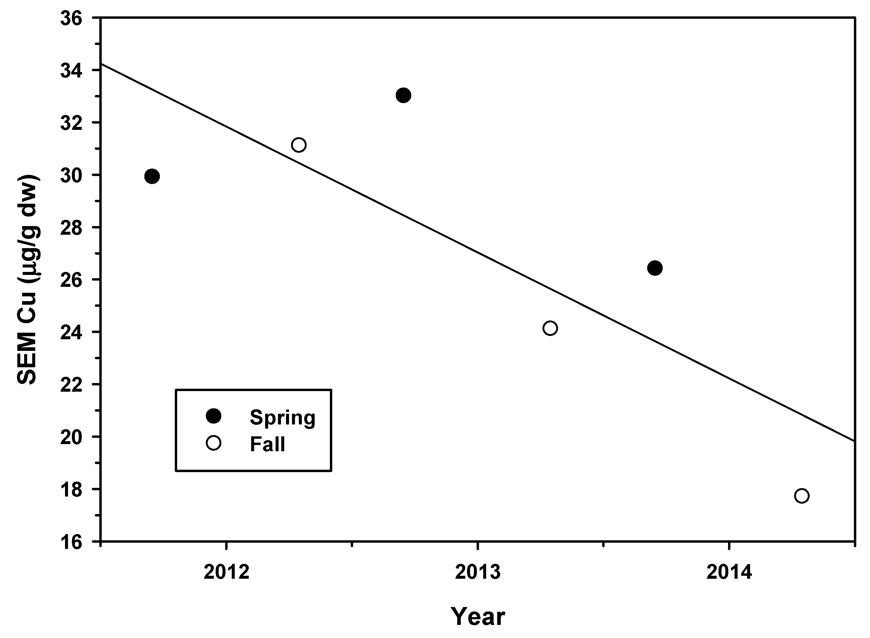
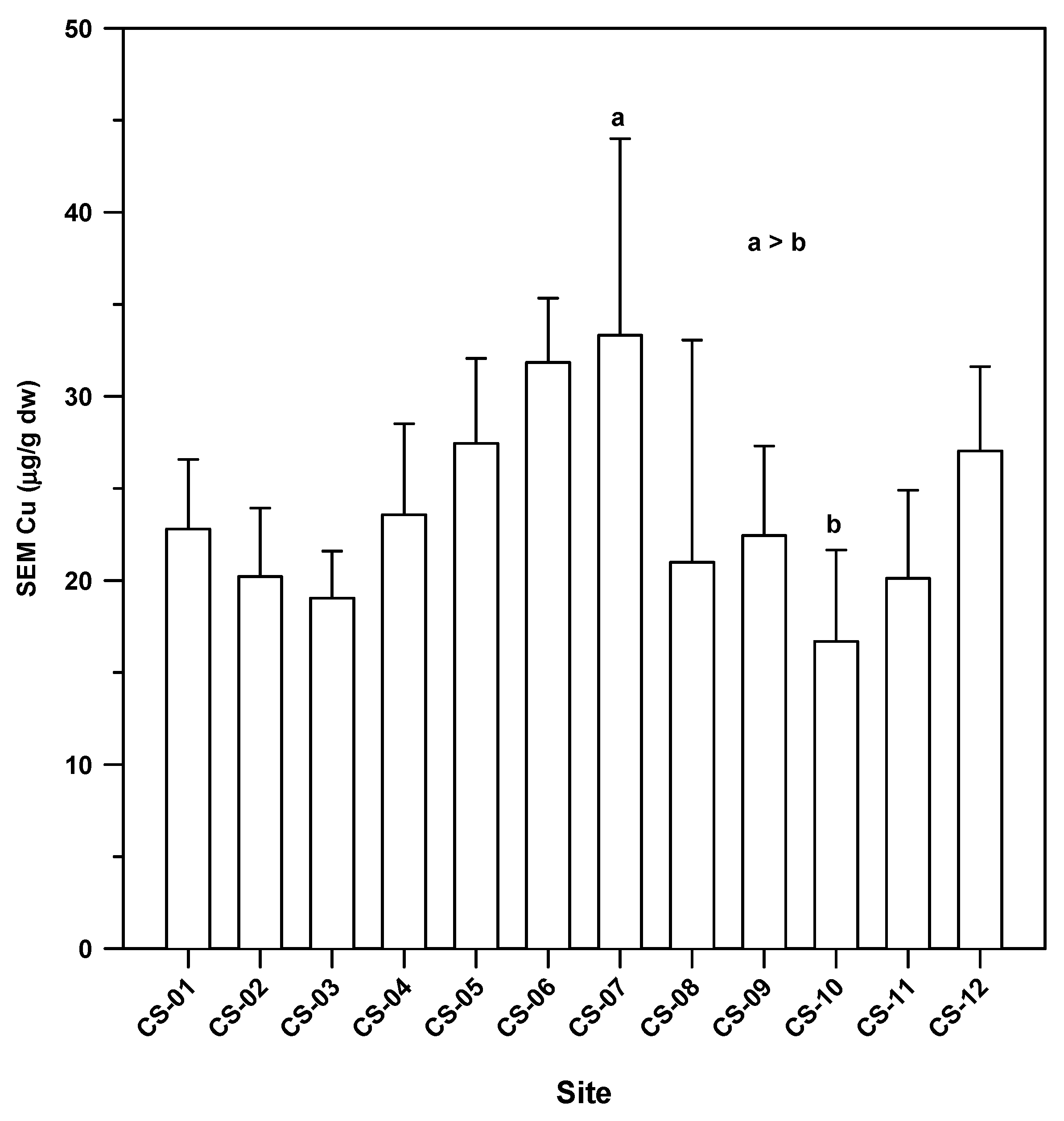
3.2. Site Trends
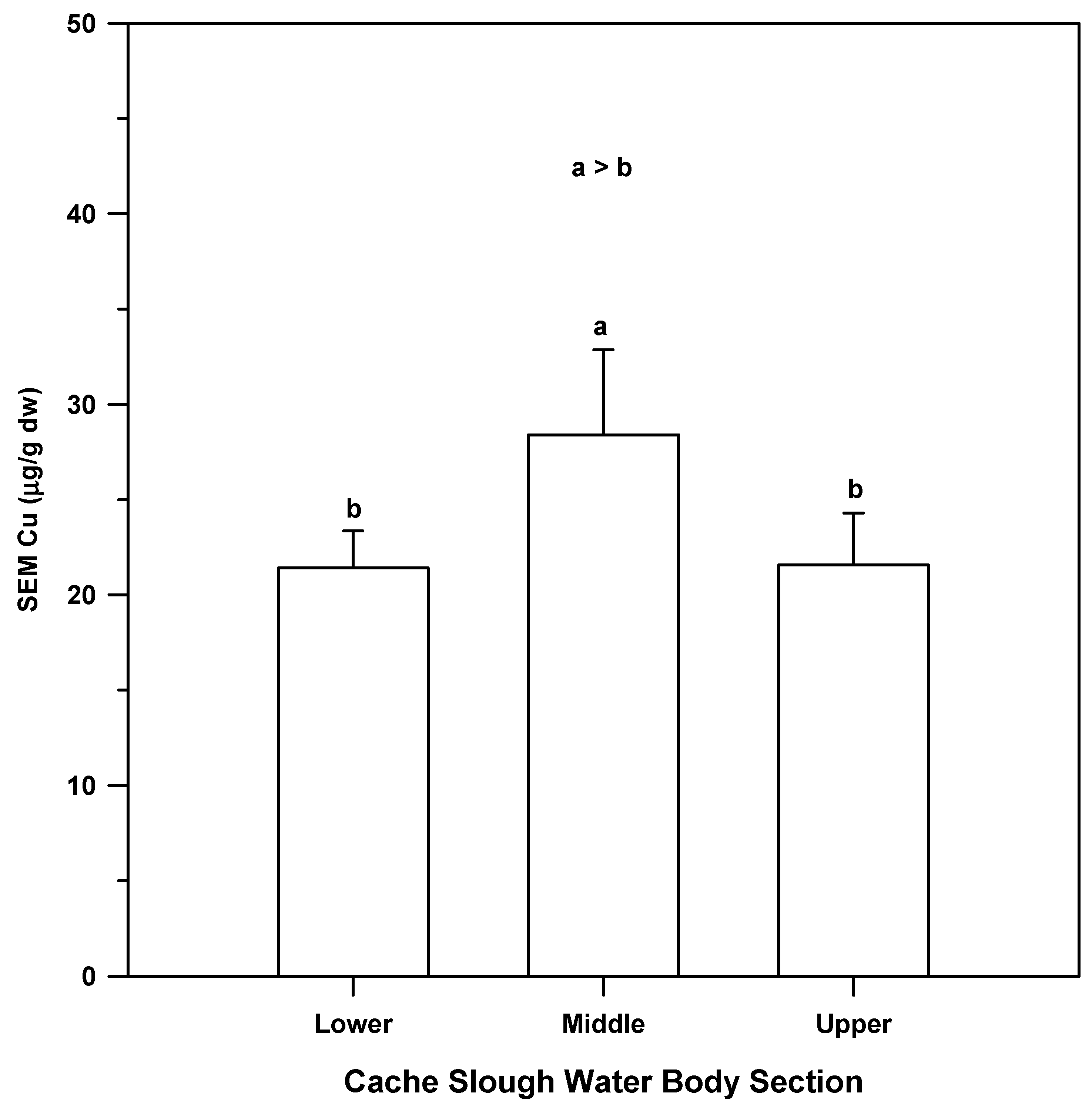
3.3. Waterbody Section Comparisons
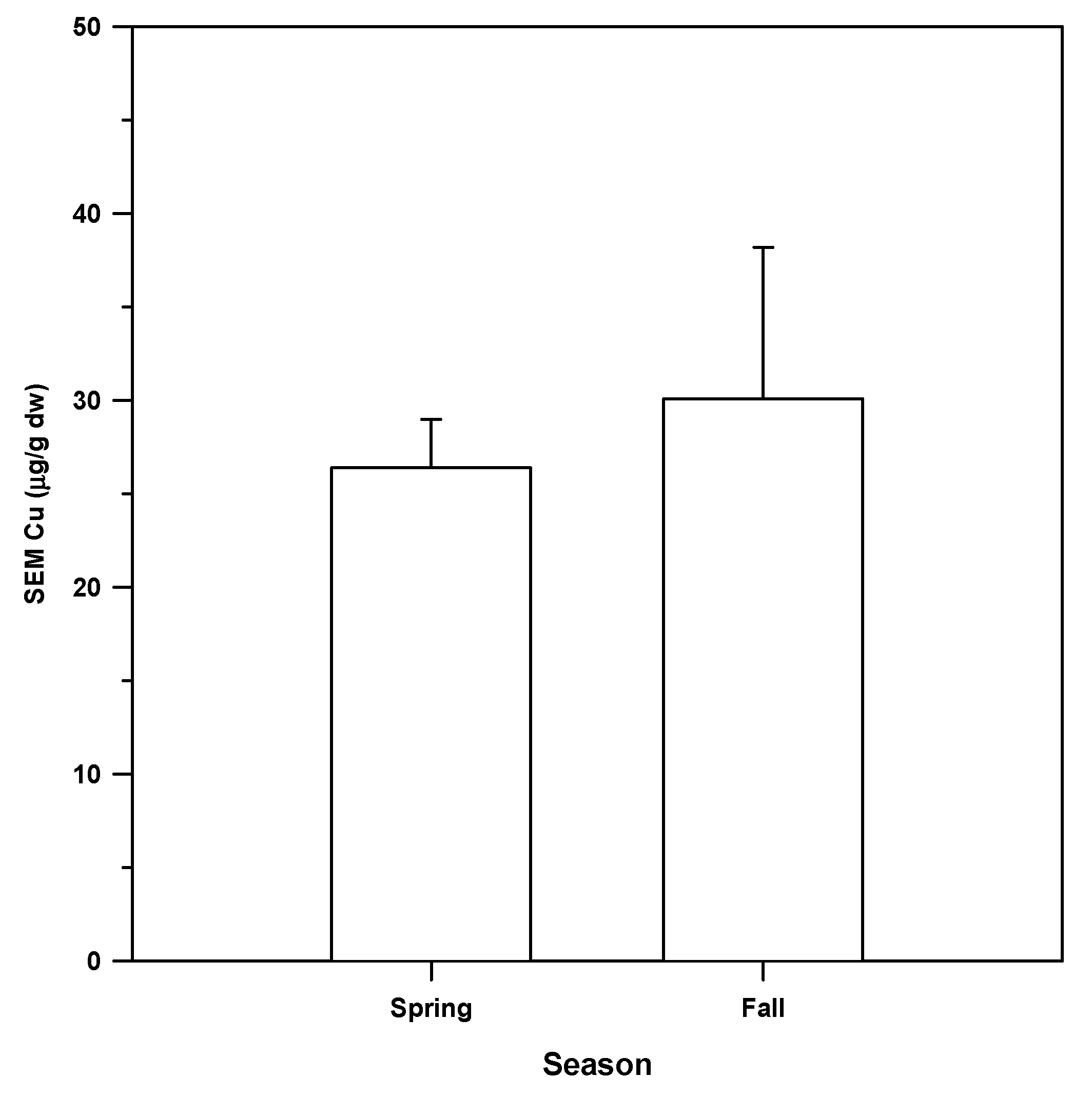
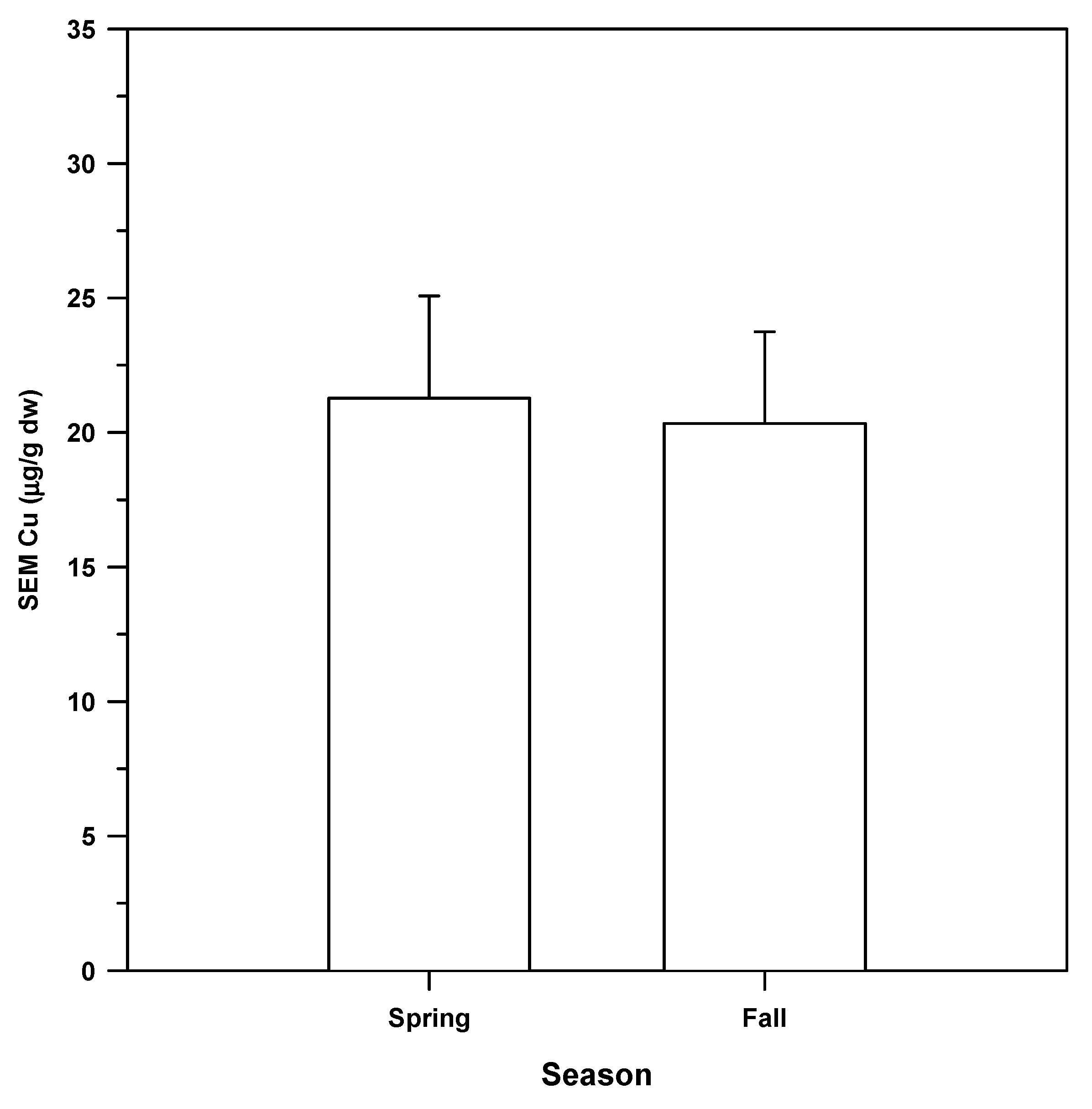
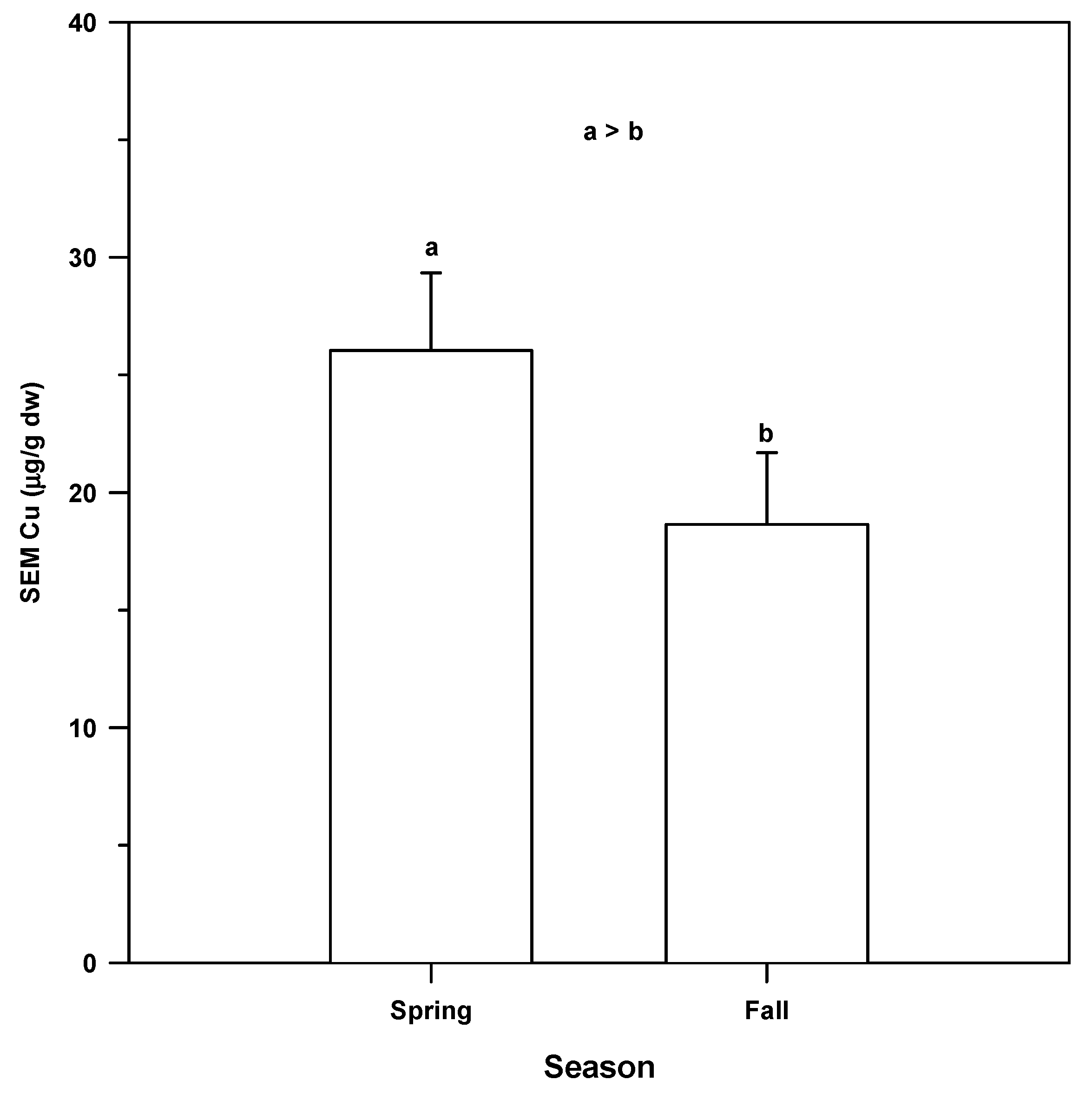
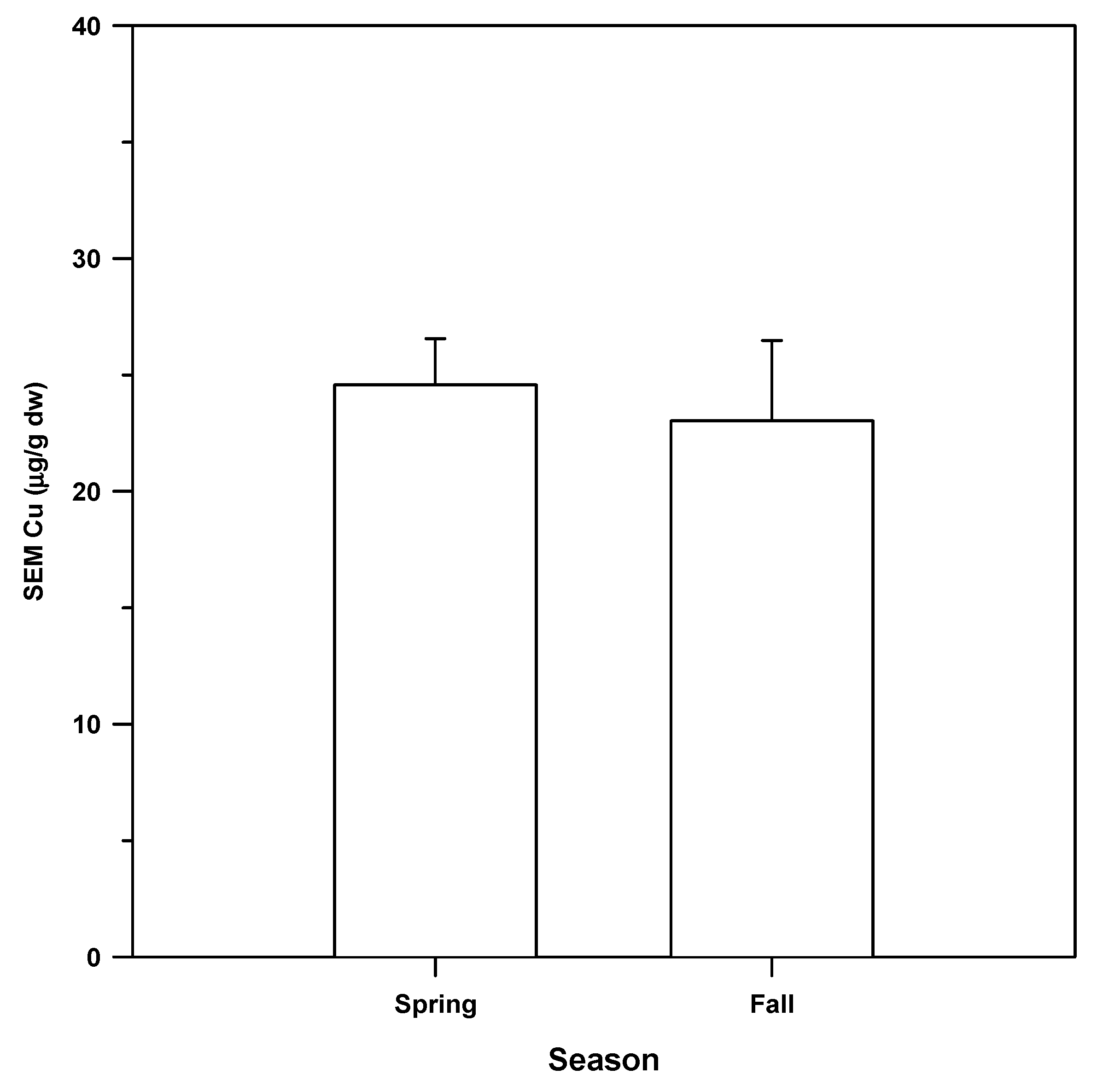
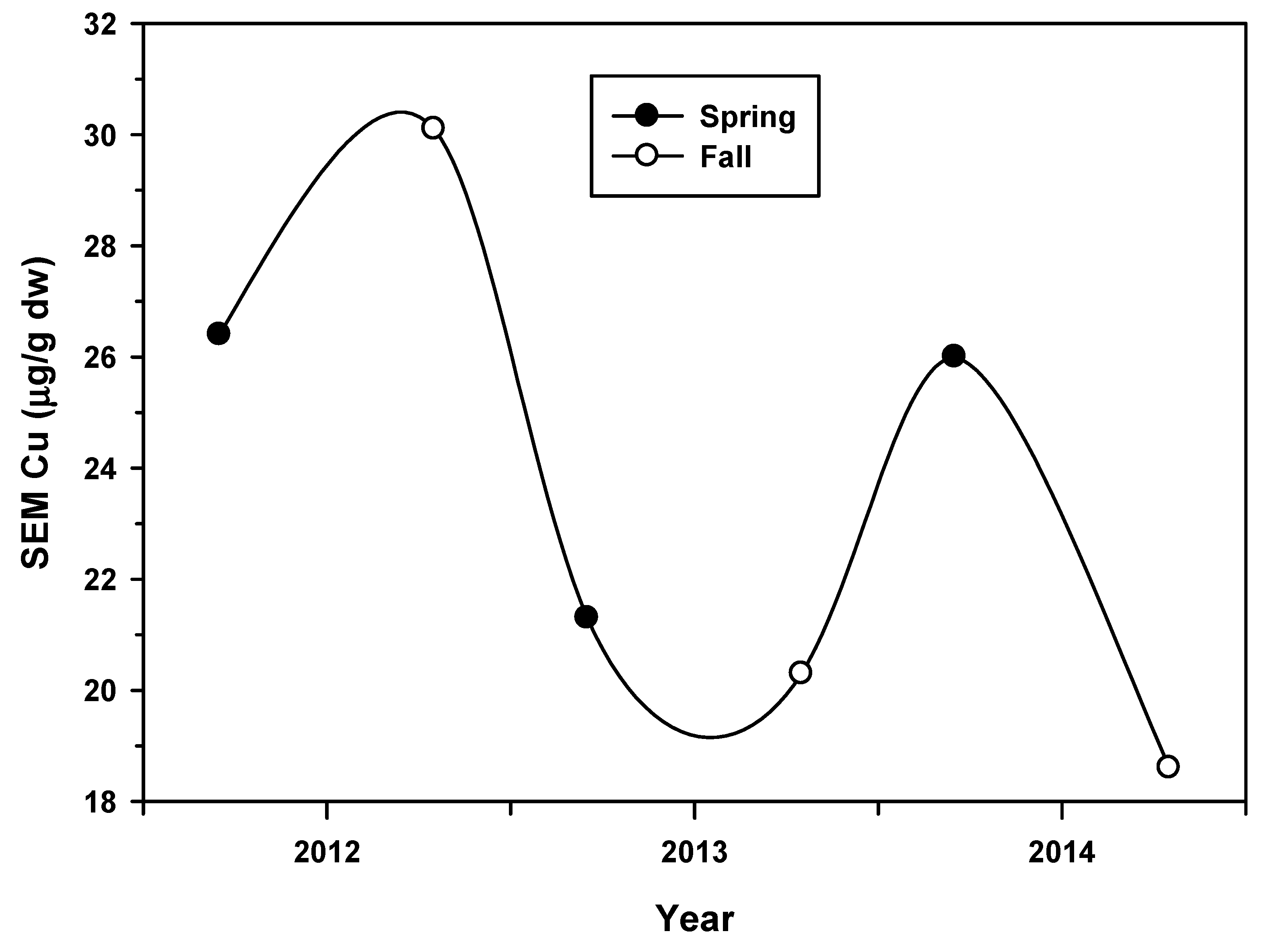
3.4. Seasonal Comparisons
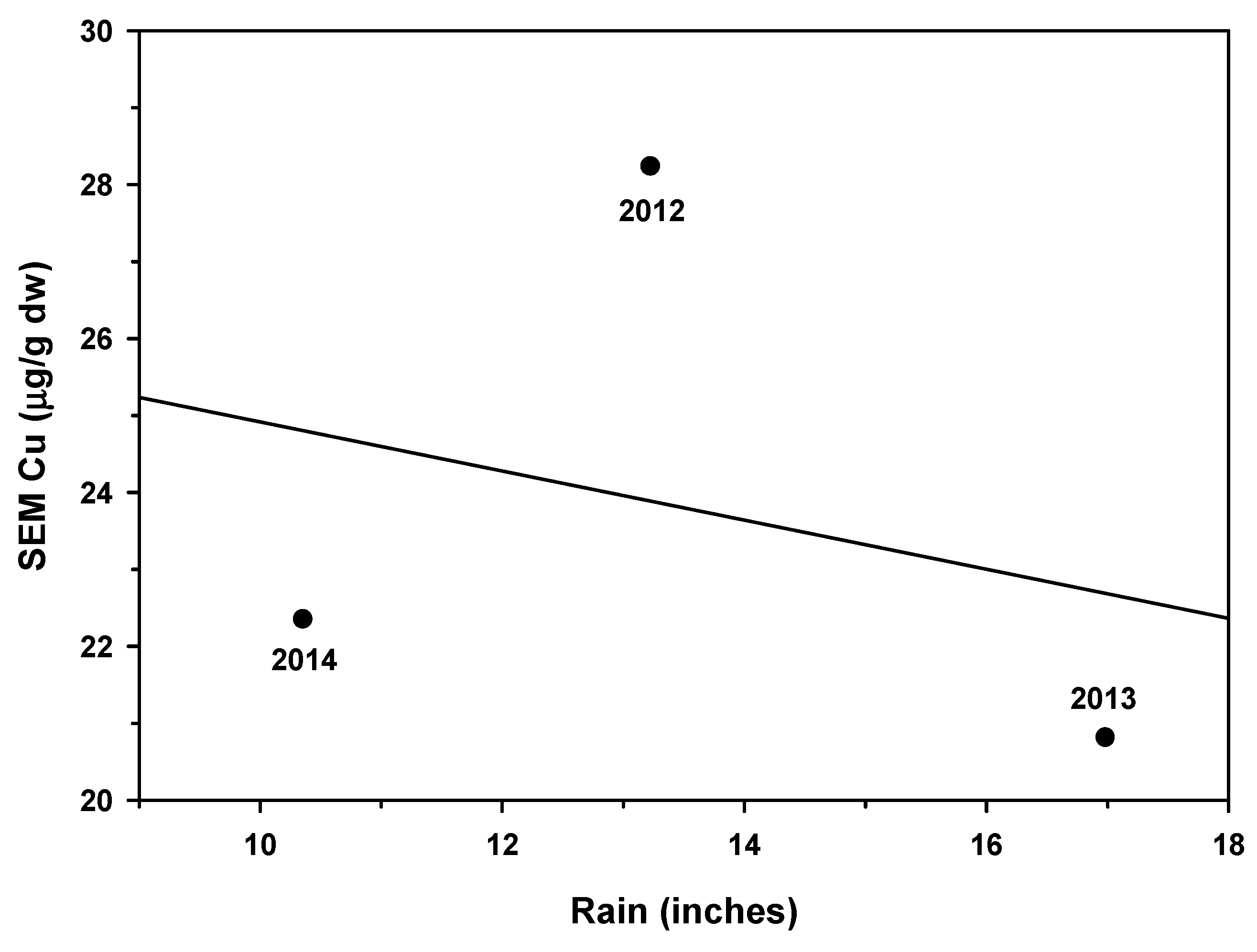
3.5. Summary of Annual Precipitation Data
4. Discussion
4.1. Comparison of Sediment SEM Copper Data from Cache Slough with Historical Data
4.2. Comparison of Sediment Total Copper Data with SEM Copper Data in Cache Slough
5. Conclusions
Author Contributions
Funding
Institutional Review Board Statement
Informed Consent Statement
Data Availability Statement
Acknowledgments
Conflicts of Interest
References
- Alves, J.P.H.; Passos, E.A.; Garcia, C.A.B. Metals and acid volatile sulfide in sediment cores for the Sergipe river estuary, northeast Brazil. J. Braz. Chem. Soc. 2007, 18, 748–758. [Google Scholar] [CrossRef] [Green Version]
- Lee, J.S.; Lee, J.H. Influence of acid volatile sulfides and simultaneously extracted metals on the bioavailability and toxicity of a mixture of sediment-associated Cd, Ni, and Zn to polychaetes Neanthes arenacoedentata. Sci. Total Environ. 2005, 338, 229–241. [Google Scholar] [CrossRef] [PubMed]
- Sahlin, S.; Agerstrand, M. Copper in Sediment; EQS Data Overview; ACES Report 28; Department of Environmental Science and Analytical Chemistry, Stockholm University: Stockholm, Sweden, 2018. [Google Scholar]
- Ditoro, D.M.; Mahony, J.D.; Hansen, D.J.; Scott, K.J.; Hicks, M.B. Toxicity of cadmium in sediments: The role of acid volatile sulfides. Environ. Toxicol. Chem. 1990, 9, 1488–1502. [Google Scholar]
- Mendez-Fernandez, L.; De Jonge, M.; Bervoets, L. Influence of sediment geochemistry on metal accumulation rates and toxicity in the aquatic oligochaete Tubifex tubifex. Aquat. Toxicol. 2014, 157, 109–119. [Google Scholar] [CrossRef] [PubMed]
- European Food Safety Authority (EFSA). Statement of the PPR Panel on a Framework for Conducting the Environmental Risk Assessment for Transition Metals When Used as Active Substances in Plant Protection Products (PPP); Report prepared for the European Commission by the EFSA; EFSA: Parma, Italy, 2020. [Google Scholar] [CrossRef]
- Hall, L.W.; Anderson, R.D. Assessing Annual, Seasonal, and Spatial Trends in Copper Sediment Concentrations from a California Agricultural Waterbody; University of Maryland: Queenstown, MD, USA, 2022. [Google Scholar]
- Hall, L.W.; Killen, W.D.; Anderson, R.D.; Alden, R.W., III. The relationship of benthic community metrics to pyrethroids, metals, and sediment characteristics in Cache Slough, California. J. Environ. Sci. Health Part A 2015, 15, 1–10. [Google Scholar] [CrossRef]
- California Department of Fish and Wildlife. Atlas of the Biodiversity of California; Biogeographic Data Branch: Sacramento, CA, USA, 2003.
- Pernigotto, G.; Gasparella, A. Classification of European Climates for Building Energy Simulation Analysis. In Proceedings of the International High Performance Building Conference, IN Paper 300, Purdue University, West Lafayette, IN, USA, 9–12 July 2018. [Google Scholar]
- International Soil Reference and Information Centre. Reference Soil Spain: Eutric Vertisol, Wageningen University and Research in Wageningen, The Netherlands. 2021. Available online: website:https://museum.isric.org/content/welcome-isric-world-soil-museum (accessed on 2 February 2022).
- U. S. Department of Agriculture, Natural Resources Conservation Service. State Soil Geographic (STATSGO2) Data Base for California. 1994. Available online: https//databasin.org/datasets/1ff4328039f948529c33e7e71bb9b5fc/ (accessed on 7 February 2022).
- Hall, L.W. Summary Cache Slough Copper Use Data; University of Maryland: Queenstown, MD, USA, 2021. [Google Scholar]
- Hall, L.W.; Dauer, D.M.; Alden, R.W., III; Uhler, A.D.; DiLoranzo, J.; Burton, D.T.; Anderson, R.D. An integrated case study for evaluating the impacts of an oil refinery effluent on aquatic biota in the Delaware River: Sediment quality triad studies. Hum. Ecol. Risk Assess. 2005, 11, 657–770. [Google Scholar] [CrossRef]
- Plumb, R.H. Procedures of Handling and Chemical Analysis of Sediment and Water Samples; Report. U. S. Army Core of Engineers; U.S. Army Engineer Waterways Experiment Station: Vicksburg, MS, USA, 1981. [Google Scholar]
- Besser, J.; Ingersoll, C.; Giesy, J. Effects of spatial and temporal variation of acid-volatile sulfide on the bioavailability of copper and zinc in freshwater sediments. Environ. Toxicol. Chem. 1996, 15, 286–293. [Google Scholar] [CrossRef]
- Burton, G.A.; Green, A.; Baudo, R.; Forbs, V.; Nguyen, L.T.H.; Janssen, R.J.; Kukkonen, J.; Leppanen, M.; Maltby, L. Characterizing sediment acid volatile sulfide concentrations in European streams. Environ. Toxicol. Chem. 2007, 26, 1–12. [Google Scholar] [CrossRef]
- Campana, O.; Rodrıguez, A.; Blasco, J. Identification of a potential toxic hot spot associated with AVS spatial and seasonal variation. Arch. Environ. Contam. Toxicol. 2009, 56, 416–425. [Google Scholar] [CrossRef]
- Patton, G.; Crecelius, E. Simultaneously Extracted Metals/Acid-Volatile Sulfide and Total Metals in Surface Sediment from the Hanford Reach of the Columbia River and the Lower Snake River; U.S. Department of Energy, Pacific Northwest National Laboratory: Richland, WA, USA, 2001. Available online: http://www.ntis.gov/ordering (accessed on 15 February 2022).
- Pignotti, E.; Guerra, R.; Covelli, S.; Fabbri, E.; Dinelli, E. Sediment quality assessment in a coastal lagoon (Ravenna, NE Italy) based on SEM-AVS and sequential extraction procedure. Sci. Total Environ. 2018, 635, 216–227. [Google Scholar] [CrossRef]
- Poot, A.; Meerman, E.; Gillissen, F.; Koelmans, A. A kinetic approach to evaluate the association of acid volatile sulfide and simultaneously extracted metals in aquatic sediments. Environ. Toxicol. Chem. 2009, 28, 711–717. [Google Scholar] [CrossRef] [PubMed]
- Pricaa, M.; Dalmacijab, B.; Rončevićb, S.; Krčmarb, D.; Bečelićb, M. A comparison of sediment quality results with acid volatile sulfide (AVS) and simultaneously extracted metals (SEM) ratio in Vojvodina (Serbia) sediments. Sci. Total Environ. 2008, 389, 235–244. [Google Scholar] [CrossRef] [PubMed]
- Van Den Berg, G.; Loch, J.; Van Der Heijdt, L.; Zwolsman, J. Vertical distribution of acid-volatile sulfide and simultaneously extracted metals in a recent sedimentation. Environ. Toxicol. Chem. 1998, 17, 758–763. [Google Scholar] [CrossRef]
- Van Den Berg, G.; Buykx, S.; Van Den Hoop, M.; Van Der Heijdt, L.; Zwolsman, J. Vertical profiles of trace metals and acid-volatile sulphide in a dynamic sedimentary environment: Lake Ketel, The Netherlands. Appl. Geochem. 2001, 16, 781–791. [Google Scholar] [CrossRef]
- Van den Hoop, M.A.G.T.; den Hollander, H.A.; Kerdijk, H.N. Spatial and seasonal variations of acid volatile sulphide (AVS) and simultaneously extracted metals (SEM) in Dutch marine and freshwater sediments. Chemosphere 1997, 35, 2307–2316. [Google Scholar] [CrossRef]
- Hall, L.W.; Killen, W.D.; Anderson, R.D.; Alden, R.W., III. The influence of physical habitat, pyrethroids, and metals on benthic community condition in an urban and residential stream in California. Hum. Ecol. Risk Assess. 2009, 15, 526–553. [Google Scholar] [CrossRef]
- Hall, L.W.; Killen, W.D.; Anderson, R.D.; Alden, R.W., III. A three-year assessment of the Influence of physical habitat, pyrethroids and metals on benthic communities in two urban Calfornia streams. J. Ecosyst. Ecography 2013, 3, 133. [Google Scholar] [CrossRef]
- Hall, L.W.; Killen, W.D.; Anderson, R.W.; Alden, R.W., III. The influence of multiple chemical and non-chemical stressors on benthic communities in a mid-west agricultural stream. J. Environ. Sci. Health Part A 2017, 52, 1008–1021. [Google Scholar] [CrossRef]
- Hall, L.W.; Anderson, R.W.; Killen, W.D.; Alden, R.W., III. An analysis of multiple stressors on resident benthic communities in a California agricultural stream. Air Soil Water Res. 2018, 11, 1–18. [Google Scholar] [CrossRef]
- Hall, L.W.; Killen, W.D.; Anderson, R.W.; Alden, R.W., III. Long term bioassessment multiple stressor study in a residential California stream. J. Environ. Sci. Health Part A 2021, 56, 1–5. [Google Scholar] [CrossRef]
- Mackie, K.A.; Muller, T.; Zikeli, S.; Kandeler, E. Long-term copper application in an organic vineyard modifies spatial distribution of soil micro-organisms. Soil Biol. Biochem. 2013, 65, 245–253. [Google Scholar] [CrossRef]
- Shull, D.H. Bioturbation. In Encyclopedia of Ocean Sciences; Elsevier: Amsterdam, The Netherlands, 2009; pp. 395–400. [Google Scholar] [CrossRef]
- Remaila, T.M.; Yin, N.; Bennett, W.W.; Simpson, S.L.; Jolley, D.F.; Weish, D.T. Contrasting effects of bioturbation on metal toxicity of contaminanted sediments resulting in misleading interpretation of the AVS-SEM metal-sulfide paradigm. Environ. Sci. Proceesses Impacts 2018, 20, 1285–1296. [Google Scholar] [CrossRef] [PubMed]
- Schloesser, D.W.; Malakauskas, D.M.; Malakauskas, S.J. Freshwater polychaete (Manayunkia speciosa) near the Detroit River western Lake Erie: Abundance and life history characteristics. J. Great Lake Res. 2016, 42, 1070–1083. [Google Scholar] [CrossRef]
- Han, F.X.; Hargreaves, J.A.; Kingery, W.L.; Huggett, D.B.; Schlenk, D.K. Accumulation, distribution and toxicity of copper in sediments of catfish ponds receiving periodic copper sulfate applications. J. Environ. Qual. 2001, 30, 912–919. [Google Scholar] [CrossRef] [PubMed]
- Baddar, Z.E.; Peck, E.; Xu, X. Temporal dispersion of copper and zinc in the sediments of metal removal constructed wetlands. PLoS ONE 2021, 16, e0255527. [Google Scholar]
- Gianessi, L.P.; Reigner, N. The Values of Fungicides in U. S. Crop Production. CropLife Foundation. 2005. Available online: www.croplifefoundation.org (accessed on 20 February 2022).


| 2012 Cu SEM (µg/g dw) | 2013 Cu SEM (µg/g dw) | 2014 Cu SEM (µg/g dw) | ||||
|---|---|---|---|---|---|---|
| Station | Spring | Fall | Spring | Fall | Spring | Fall |
| CS-01 | 28.6 | 28.0 | 18.4 | 17.8 | 22.3 | 21.7 |
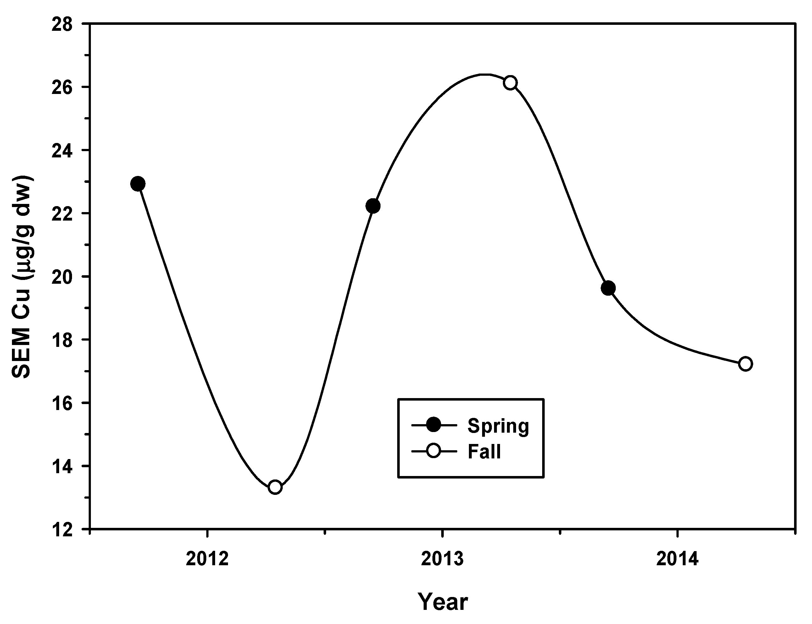
| CS-02 | 22.9 | 13.3 | 22.2 | 26.1 | 19.6 | 17.2 |
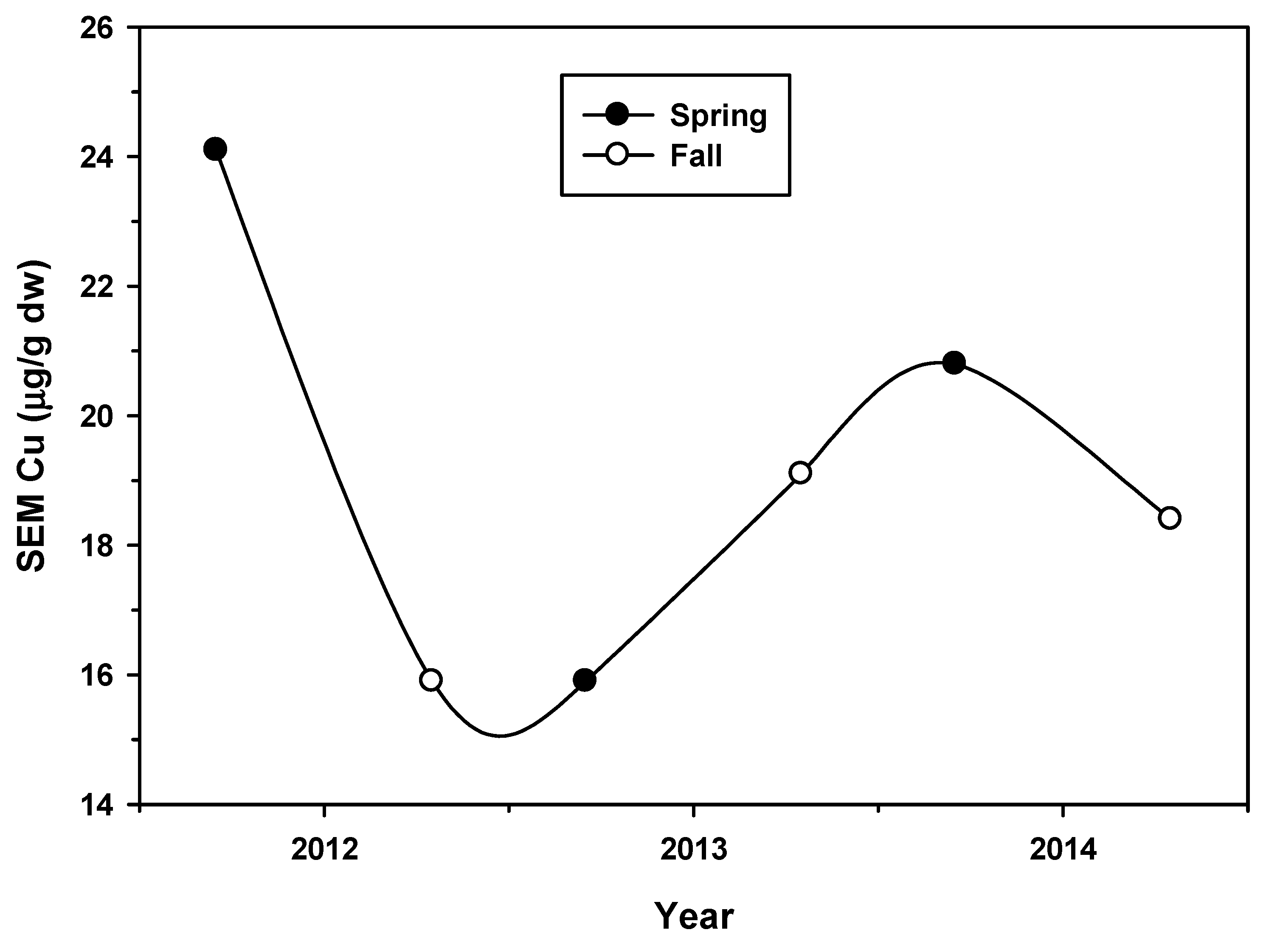
| CS-03 | 24.1 | 15.9 | 15.9 | 19.1 | 20.8 | 18.4 |
| CS-04 | 32.4 | 28.6 | 23.5 | 22.2 | 17.8 | 16.9 |
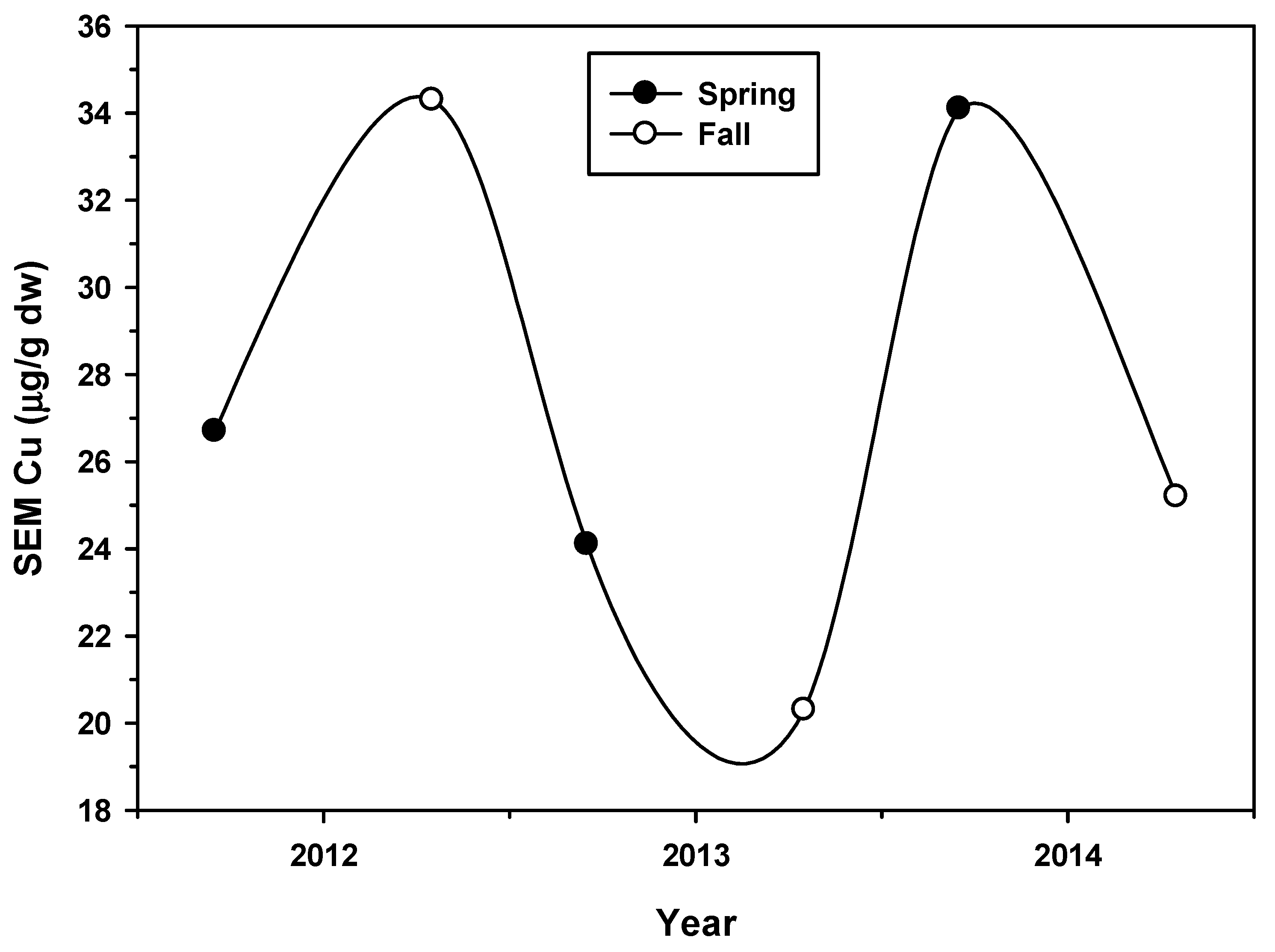
| CS-05 | 26.7 | 34.3 | 24.1 | 20.3 | 34.1 | 25.2 |
| CS-06 | 32.4 | 38.8 | 29.9 | 28.0 | 34.3 | 27.6 |
| CS-07 | 29.2 | 59.1 | 25.4 | 27.3 | 34.2 | 24.7 |
| CS-08 | 26.1 | 46.4 | 9.5 | 8.9 | 25.2 | 9.8 |
| CS-09 | 25.4 | 31.1 | 20.3 | 21.0 | 23.6 | 13.2 |
| CS-10 | 17.2 | 8.9 | 19.1 | 11.4 | 26.2 | 17.3 |
| CS-11 | 21.6 | 25.4 | 14.0 | 17.8 | 27.9 | 14.0 |
| CS-12 | 29.9 | 31.1 | 33.0 | 24.1 | 26.4 | 17.7 |
| Year | Season | n | Mean | Std Dev | Range | Min | Max | Median |
|---|---|---|---|---|---|---|---|---|
| 2012 | Spring | 12 | 26.4 | 4.51 | 15.2 | 17.2 | 32.4 | 26.4 |
| Fall | 12 | 30.1 | 14.0 | 50.2 | 8.90 | 59.1 | 29.9 | |
| 2013 | Spring | 12 | 21.3 | 6.59 | 23.5 | 9.50 | 33.0 | 21.3 |
| Fall | 12 | 20.3 | 5.91 | 19.1 | 8.90 | 28.0 | 20.7 | |
| 2014 | Spring | 12 | 26.0 | 5.73 | 16.5 | 17.8 | 34.3 | 25.7 |
| Fall | 12 | 18.6 | 5.28 | 17.8 | 9.80 | 27.6 | 17.5 |
| Water | Precipitation (Inches) | Water Year | Sum % of 30 | |||||||||||
|---|---|---|---|---|---|---|---|---|---|---|---|---|---|---|
| Year | OCT | NOV | DEC | JAN | FEB | MAR | APR | MAY | JUN | JUL | AUG | SEP | Sum of Rain | Year Mean ** |
| 2011 | 1.75 | 2.65 | 5.52 | 1.36 | 3.88 | 7.00 | 0.08 | 1.40 | 1.14 | 0.00 | 0.00 | 0.00 | 24.78 | 125 |
| 2012 * | 1.72 | 0.87 | 0.07 | 2.52 | 0.94 | 4.45 | 2.65 | 0.00 | 0.01 | 0.00 | 0.00 | 0.00 | 13.23 | 67 |
| 2013 * | 1.28 | 4.33 | 6.46 | 1.06 | 0.26 | 1.59 | 0.58 | 0.57 | 0.31 | 0.00 | 0.00 | 0.55 | 16.99 | 86 |
| 2014 * | 0.00 | 0.82 | 0.38 | 0.20 | 4.49 | 1.93 | 1.97 | 0.01 | 0.00 | 0.02 | 0.00 | 0.54 | 10.36 | 51 |
| 2015 | 0.37 | 1.28 | 7.63 | 0.01 | 2.28 | 0.16 | 1.81 | 0.19 | 0.07 | 0.00 | 0.00 | 0.00 | 13.80 | 68 |
| Location | Water Body/Primary Surrounding Land Use | Depositional Areas Targeted? | # of Sites Sampled & Frequency | SEM Cu (Min–Max, Mean) | Reference |
|---|---|---|---|---|---|
| Western Montana, USA | Upper Clark Fork River and Milltown Reservoir/Primarily forested but with some inputs from agriculture or Cu mining upstream; some agricultural influence | Not reported | 3 sections, 7 total sites sampled once from composite samples (1 of 7 sites agr) | RC (reference): (1.91–1.91, 1.91) a Milltown Reservoir: (35.0–902, 265) Upper Clark Fork: (655–655, 655) Upper Clark Fork Agriculture (CF4): (36.2–36.2, 36.2) | [16] |
| Sweden, Denmark, England, Finland, Belgium, France, Germany, and Italy | SW Sweden/Agriculture b E Denmark/Agriculture S England & Wales/Agriculture S Finland/Agriculture S Belgium/Agriculture | Yes (sand grain size and smaller) | Sweden: 3 sites, 1 composited sample each site, sampled once c Denmark: 6 sites England/Wales: 16 sites Finland: 5 sites Belgium: 6 sites | Sweden: (2.29–8.90, 4.85) Denmark: (1.84–110.2, 5.28) England/Wales: (7.12–25.9, 15.4) Finland: (1.21–41.5, 13.0) Belgium: (3.50–22.7, 11.2) | [17] |
| Sweden, Denmark, England, Finland, Belgium, France, Germany, and Italy | N France/Agriculture W & S Germany/Agriculture N Italy/Agriculture | Yes | France: 12 sites Germany: 9 sites Italy: 2 sites | France: (0.064–20.8, 8.23) Germany: (1.97–76.1, 15.7) Italy: (3.05–3.56, 3.30) | |
| Guadalete Estuary, SW Spain (tidal sites) | Site G1/Harbor/Port Sites G2–G3/Agriculture Sites S1-S7/Mouths of agriculture drains | Yes (most samples < 63 um) | 10 sites with 3 replicates/site, sampled twice (Aug 2002 & Mar 2003) | Site G1: (4.4–170, 46.4) Sites G2–G3: (10.8–16.5, 14.0) Sites S1-S7: (5.7–21.0, 14.4) | [18] |
| Washington State Desert | Hanford Reach (Columbia River)/Desert Priest Rapids Dam (Columbia River)/Agr McNary Dam (Columbia River)/Agriculture Ice Harbor Dam (Snake River)/Agriculture | Not reported | 4 sites sampled 2–3 times over 3 years 6 sites sampled 2–3 times over 3 years 6 sites sampled 2–3 times over 3 years 3 sites sampled 2 times over 2 years | Hanford Reach Site (desert): (5.27–12.6, 8.63) Priest Rapids Dam Sites: (4.38–30.5, 17.7) McNary Dam Sites: (6.80–20.9, 15.9) Ice Harbor Dam: (4.64–15.7, 12.3) | [19] |
| Ravenna, NE Italy (tidal sites) | Pialassa Piomboni (coastal lagoon)/Primary freshwater input from agriculture | Not reported | 50 sites sampled once | Pialassa Piomboni: (0.318–89.0, 6.35) | [20] |
| SE Netherlands | Beekloop (headwater stream)/Agriculture d | Not reported | 4 sites sampled once with 3 replicates per site | Sites L1–4: (19.1–76.3, 53.2) | [21] |
| N Serbia | Various rivers, canals, streams/Agriculture Various rivers, canals, streams/Urban | Yes | 9 urban sites sampled twice in one year 3 urban sites sampled twice in one year | Agriculture: (6.35–96.6, 45.4) e Urban: (12.7–23.5, 17.6) | [22] |
| SW Netherlands | Meuse/Rhine River Delta/Agriculture f | Yes | 4 sites sampled twice in Nov 1995 and once in Jun 1996 | Sites 1–4: (19.1–76.3, 56.7) | [23] |
| N Netherlands | Lake Ketel/Agriculture (some urban upstream) | Yes (most sediment < 63 um) | 4 sites (10 reps per site) sampled once | Sites A–D: (13.3–58.5, 35.3) | [24] |
| Netherlands/Belgium | Various Coastal Sites (11–20 km offshore) Various Urban Sites | Not reported | 8 sites sampled once 10 sites sampled once | Coastal sites: (0.635–2.52, 1.27) Urban sites: (1.27–49.6, 17.1) | [25] |
| Netherlands/Belgium | Various Agriculture Sites (some urban upstream) | Not reported | 3 sites sampled once | Agriculture sites: (10.8–71.8, 34.5) | |
| Antioch, California State | Lower Kirker Creek/Urban Upper Kirker Creek/Agriculture g | Yes | 14 sites with composite samples collected once for 2 years | 12 Urban Sites: (0.191–12.6, 3.05) 2 Agriculture Sites: (0.191–12.4, 4.21) | [26] |
| Salinas, California State | Alisal, Gabilon and Natividad Creeks/Urban with some agriculture | Yes | 13 sites with composite samples collected once/year for 3 years | 11 Urban Sites h (3.62–20.6, 8.49) 2 Agriculture Sites: (2.67–8.26, 5.46) | [27] |
| N Illinois State | Big Bureau Creek/Agriculture | Yes | 12 sites with composite samples collected once/year for 3 years | Sites 1–12: (2.54–7.63, 4.63) | [28] |
| Santa Maria, California State | Santa Maria River, Osco Flaco Creek, Orcutt Creek and unnamed drainages/Agriculture | Yes | 12 sites with composite samples collected once/year for 3 years | Sites 1–12 h (7.63–20.3, 11.5) | [29] |
| Pleasant Grove, California State | Upper Pleasant Grove Creek and Tributaries/Urban Lower Pleasant Grove Creek/Agriculture | Yes | 21 sites with composite samples collected once/year for 10 years | 18 Urban Sites: (0.508–252, 21.5) 3 Agriculture Sites: (0.191–21.9, 6.94) | [30] |
| Metric | Total Copper | SEM Copper | Results |
|---|---|---|---|
| Range of mean seasonal concentrations | 37–46 µg/g dw | 18.6–30.1 µg/g dw | Mean SEM copper seasonal range lower |
| Significant site trends | CS-04 downward trend | CS-04, CS-09, CS-12 downward trend | More sites show downward trend with SEM copper; no sites showed increasing concentrations |
| Significant site comparisons | Both CS-06 and CS-05 showed higher values that 2 to 3 upstream sites | CS-07 higher than upstream site CS-10 | More significant differences among sites for total copper |
| Significant water body section comparisons | Concentrations in middle section higher than upper section but not lower section | Concentration in middle section higher than both upper and lower section | Similar results showing higher concentrations in middle water body section |
| Significant seasonal differences | No seasonal differences for both spring and fall for 2012 and 2013 but spring concentrations higher in 2014 | No seasonal differences for both spring and fall for 2012 and 2013 but spring concentrations higher in 2014 | Same results |
| Significant differences with seasons combined for all years | No significant differences | No significant differences | Same results |
| Significant relationship to precipitation | No relationship to precipitation | No relationship to precipitation | Same results |
Publisher’s Note: MDPI stays neutral with regard to jurisdictional claims in published maps and institutional affiliations. |
© 2022 by the authors. Licensee MDPI, Basel, Switzerland. This article is an open access article distributed under the terms and conditions of the Creative Commons Attribution (CC BY) license (https://creativecommons.org/licenses/by/4.0/).
Share and Cite
Hall, L.W., Jr.; Anderson, R.D. Trends Analysis of Simultaneously Extracted Metal Copper Sediment Concentrations from a California Agricultural Waterbody including Historical Comparisons with Other Agricultural Waterbodies. Agriculture 2022, 12, 540. https://doi.org/10.3390/agriculture12040540
Hall LW Jr., Anderson RD. Trends Analysis of Simultaneously Extracted Metal Copper Sediment Concentrations from a California Agricultural Waterbody including Historical Comparisons with Other Agricultural Waterbodies. Agriculture. 2022; 12(4):540. https://doi.org/10.3390/agriculture12040540
Chicago/Turabian StyleHall, Lenwood W., Jr., and Ronald D. Anderson. 2022. "Trends Analysis of Simultaneously Extracted Metal Copper Sediment Concentrations from a California Agricultural Waterbody including Historical Comparisons with Other Agricultural Waterbodies" Agriculture 12, no. 4: 540. https://doi.org/10.3390/agriculture12040540