Algorithm for Extracting the 3D Pose Information of Hyphantria cunea (Drury) with Monocular Vision

Abstract

Currently, the robustness of pest recognition algorithms based on sample augmentation with two-dimensional images is negatively affected by moth pests with different postures. Obtaining three-dimensional (3D) posture information of pests can provide information for 3D model deformation and generate training samples for deep learning models. In this study, an algorithm of the 3D posture information extraction method for Hyphantria cunea (Drury) based on monocular vision is proposed. Four images of every collected sample of H. cunea were taken at 90° intervals. The 3D pose information of the wings was extracted using boundary tracking, edge fitting, precise positioning and matching, and calculation. The 3D posture information of the torso was obtained by edge extraction and curve fitting. Finally, the 3D posture information of the wings and abdomen obtained by this method was compared with that obtained by Metrology-grade 3D scanner measurement. The results showed that the relative error of the wing angle was between 0.32% and 3.03%, the root mean square error was 1.9363, and the average relative error of the torso was 2.77%. The 3D posture information of H. cunea can provide important data support for sample augmentation and species identification of moth pests.

1. Introduction

Hyphantria cunea (Drury) belongs to Lepidoptera, Arctiidae. It is a pest that resides worldwide, feeds on miscellaneous plants, reproduces considerably, may cause devastating damage to agricultural and forestry crops, and is difficult to control and manage [1]. Acquisition of occurrence information of H. cunea is an important prerequisite for its early detection and accurate control. With the development of machine vision technology, its application in pest identification is increasingly common. However, it remains difficult to identify multi-pose pests [2]. Lv et al. [3] developed an identification method for multi-objective rice light-trap pests based on template matching. They obtained an accurate rate of multi-template matching of 83.1%, which was higher than the accurate rate of single template matching (59.9%). Li et al. [4,5,6] developed three methods for multi-pose pest classification using two-dimensional (2D) image information. These methods included feature extraction and classification of multi-pose pests based on machine vision, automatic identification of orchard pests based on posture description, and fuzzy classification of orchard pest posture based on Zernike moments. The classification methods achieved a good recognition effect in laboratory conditions.

In recent years, deep learning has been gradually applied to improve the identification accuracy of pests because of its outstanding advantages. Wen et al. [2] used the structural similarity index to estimate the posture of apple moth pests, built a deep neural network for moth identification based on improved pyramidal stacked denoising autoencoder architecture, and an achieved identification accuracy of 96.9%. Ding and Taylor [7] proposed an automatic detection pipeline based on deep learning for identifying codling moths in field traps and achieved a recognition accuracy of 93.1%. Chen et al. [8] proposed a method for segmentation and counting of aphid nymphs on pak choi leaves using convolutional neural networks, and the counting precision achieved was high. Cheng et al. [9] proposed a pest identification method based on deep residual learning with complex farmland background; the classification accuracy of 10 crop pests was 98.67%. Xie et al. [10] designed a multilevel fusion classification framework of field crop pests that was aligned with the multilevel deep feature learning model, and the results on 40 common pest species in field crops showed that the multilevel learning feature model outperformed the state-of-the-art methods of pest classification. Shen et al. [11] developed an improved inception network to extract feature maps and used Faster Region-Based Convolutional Neural Network (R-CNN) to classify stored-grain insects. They achieved a mean average precision of 88%. Sun et al. [12] trained a Faster R-CNN model optimized with the K-means clustering algorithm to detect the red turpentine beetle with unconstrained postures. The area under the curve for object and trap on all test sets reached 0.9350 and 0.9722, respectively. A two-layer Faster R-CNN was proposed to detect brown rice planthopper (Nilaparvata lugens Stal). The accuracy and recall rate of the detection model reached 94.5% and 88.0%, respectively, and the detection result was much better than that of the YOLO v3 algorithm [13]. Wang et al. [14] proposed a novel two-stage mobile vision-based cascading pest detection approach (DeepPest), and the pest images were classified into crop categories based on multi-scale contextual information. Then, a multi-projection pest detection model was trained with crop-related pest images. Jiao et al. [15] proposed an anchor-free region convolutional neural network (AF-RCNN) to classify pests via an end-to-end way. The AF-RCNN obtained 56.4% mean average precision and 85.1% mean recall on a dataset of 24 pests. Khanramaki et al. [16] used an ensemble of deep learning models to classify three citrus pests. Diversity at the classifier, feature, and data levels were comprehensively considered, and the recognition accuracy was 99.04%.

The main problem in the deep learning models for pest identification is the lack of a large number of training samples. Currently, 2D images are primarily used for geometric and light intensity transformation in samples augmentation. The posture diversity of the pest training samples is limited, which creates difficulties in meeting the requirements for deep learning training. Deformation simulation based on three-dimensional (3D) data does not cause information loss when the object posture changes and has strong robustness in multi-pose object recognition [17,18].

The 3D technology application in insects primarily includes 3D model reconstruction, insect flight posture, and 3D posture estimation. Machine vision, confocal laser scanning microscope (CLSM), magnetic resonance imaging (MRI), and micro-computerized tomography (micro-CT) are the primary methods for 3D model reconstructions of insects. The 3D reconstruction of insects based on machine vision primarily uses monocular or stereo vision with a rotating platform to acquire insect images and 3D reconstruction software to achieve the 3D reconstruction of adult insects [19,20,21,22,23]. CLSM, MRI, and micro-CT are primarily used to reconstruct 3D models of insect local organs or larvae [24,25,26,27,28,29,30]. In the aspect of insect flight posture, the kinematic parameters of insect hovering and autonomous flight are obtained for the development of micro-bionic aircraft. Yu and Sun used numerical methods to solve Navier–Stokes equations to study the aerodynamic interaction between the wings and the body on both sides of a model insect during flight. When hovering, the influence of the interaction between the wings and the body and the wings was less than 3% and less than 2%, respectively [31]. Chen and Sun [32,33] reconstructed and analyzed the kinematic parameters of the wings and body of the fly in the process of rapid take-off and autonomous flight based on the contour information of the image obtained by three high-speed cameras placed in orthogonal position. Huang [34] reconstructed the 3D shells of insects and used their projection to estimate the insect posture. The flapping angle curve was obtained by using the fly data set to verify the posture estimation algorithm, and the flapping and swing angles had similar regular variations. Lv et al. [35] proposed an effective method of obtaining target 3D posture based on lidar, which can simplify the recognition and improve the recognition rate. There are few studies on 3D posture applied to insect recognition. Zhang et al. [36] manually marked the key points of insect wings, extracted the spatial coordinates of the marked feature points of moth forewings based on the Harris corner detection method, and obtained the angle of the forewings through calculation. Moreover, Chen et al. [37] designed an insect recognition device and method based on 3D posture estimation.

Three-dimensional posture information extraction is an important basis for a 3D model of insect deformation. However, so far, there are few studies on the extraction of 3D insect postures [36], and these are primarily based on the artificial marking method to extract 3D insect postures. In this study, we proposed a scheme to extract 3D posture information of H. cunea based on machine vision and quantified the 3D posture characteristics of H. cunea, which provides an information source for the subsequent construction of the 3D deformation calculation method for feature-preserving augmentation of moth pest samples. Additionally, the method presented in the study provides a view of generating a large number of 3D posture dataset for current popular deep learning models in an effective way.

2. Materials and Methods

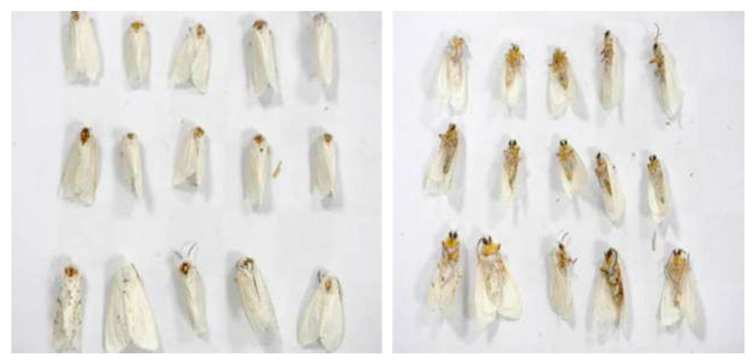
2.1. Sampling of H. cunea

A self-developed automatic pest monitoring device was used to obtain the samples of H. cunea from Xiaotangshan Precision Agriculture Demonstration Base in Changping District, Beijing, China. We aimed to collect samples of H. cunea with different postures so that the images of the samples could facilitate subsequent data processing and improve accuracy.

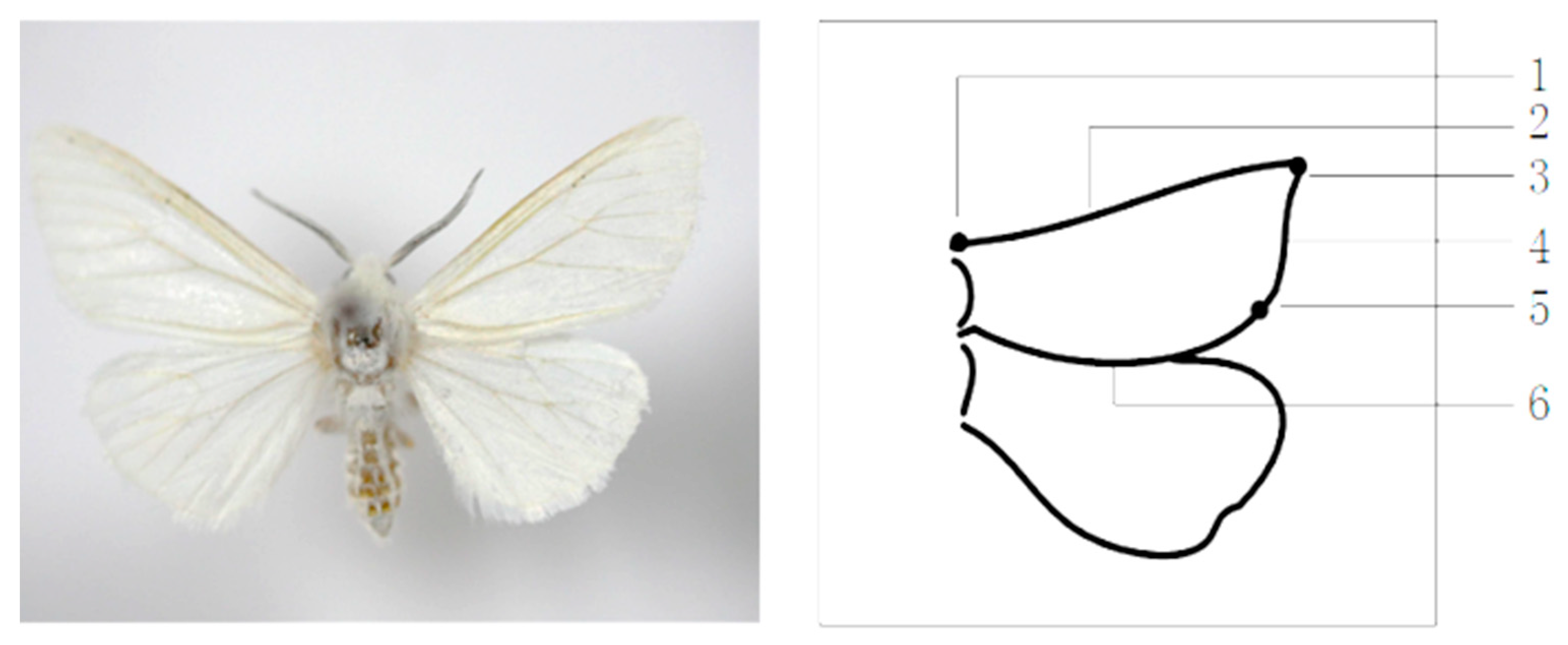
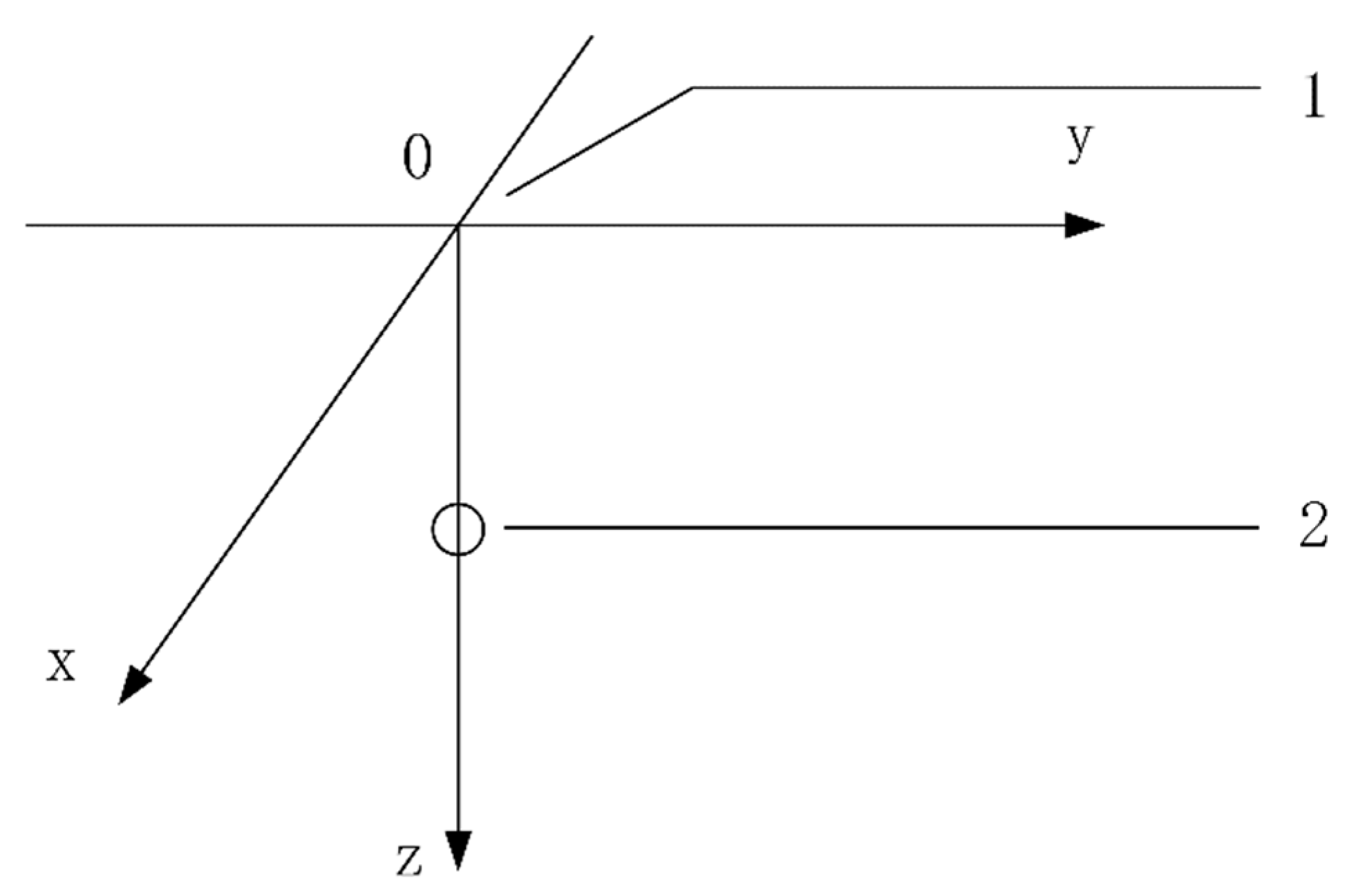
2.2. Definition of 3D Posture Information of H. cunea

The posture change of Lepidopteran pests is caused by the rotation of wings around the humeral angle and deformation of the torso. According to the characteristics of shape and posture changes of the H. cunea, the 3D posture information of the H. cunea was divided into wings and torso. The angle of the wings on the dorsal side of the insect, namely the intersection line of the plane where the wings are, is the 3D posture of the insect wing. Figure 1 shows images of the ventral and dorsal sides of H. cunea samples in various postures.

The wings of H. cunea include the fore and hind wings, which are nearly triangular and comprise three margins and three angles. The three angles are the humeral, apical, and anal angles (Figure 2). The fore wings of H. cunea cover the hind wings in a general posture, and the fore and hind wings are almost in the same plane. Moreover, the shape of the hind wings exposed to the outside is similar to that of the fore wings and is almost triangular. In this experiment, the hind wings were ignored: the fore and hind wings were combined into a plane calculation, and three inflection points of the wing contour curve were selected as three key points. The positions of the three points in the study were not the strictly defined humeral, apical, and anal angles of the front wing.

The torso part of a moth pest includes the head, thorax, and abdomen. Figure 3 shows the images of the abdomen of H. cunea in different postures. The torso posture change is caused by abdominal distortion or bending deformation. The posture of H. cunea is primarily of two types. The first is with the wings open: the angle between the two wings is more than 180°, and every angle of the abdomen is exposed. The second is with the wings retracted: the angle between the two wings is less than 180°, and the abdomen is visible in the front, but the back is occluded. Therefore, it is necessary to extract the 3D posture information of the torso using two methods according to whether the wing angle is greater than 180°.

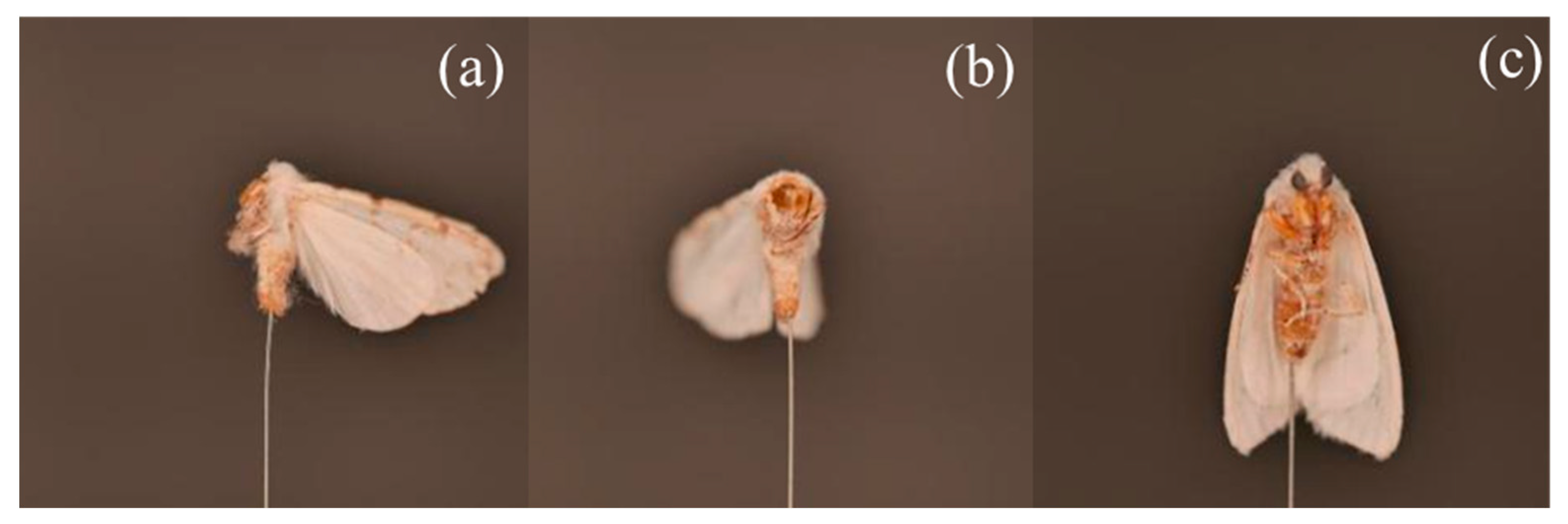
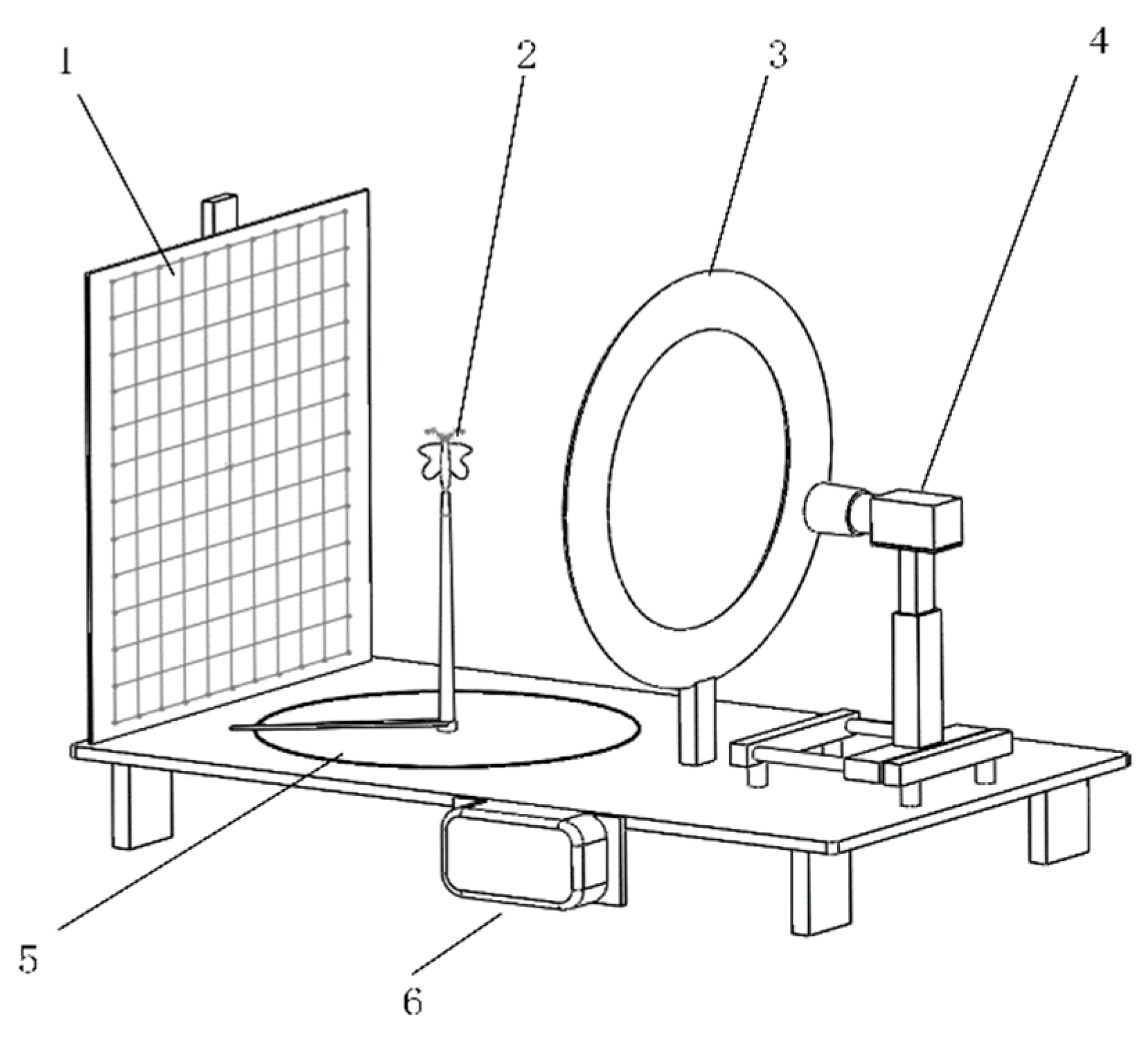
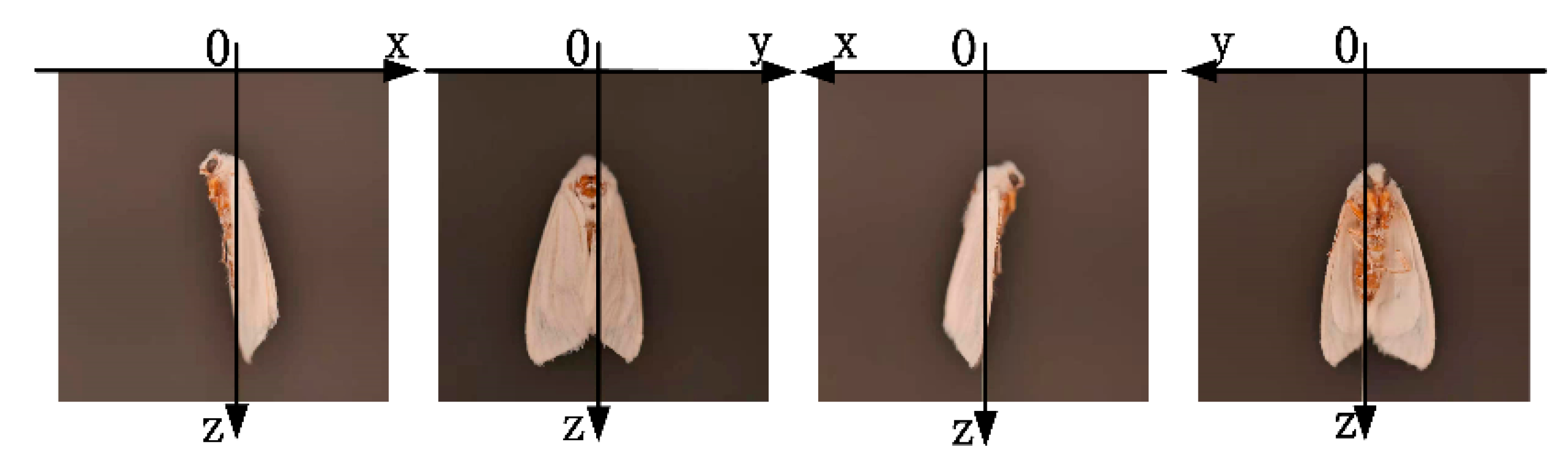
2.3. Image Data Acquisition

The image acquisition platform is shown in Figure 4. The background plate was a white square paper with a 1 cm unit, and the insect specimens were fixed vertically to the axis of rotation. A background plate was used for converting pixel coordinates to corresponding actual coordinates in the later stage. In the formal collection of H. cunea sample images, the square paper plate with a white background was replaced with a black background plate to facilitate the differentiation between the background and the H. cunea, and to extract the features of H. cunea. The insect needle and the axis of rotation were connected by a graduated rotating platform, and the insect needle could rotate along with the rotating platform. The camera used was a Panasonic DMC-GH4 (Panasonic, Suzhou, China) with a resolution of 2448 × 2448 pixels. The focal length of the camera was 60.0 mm, and the aperture value was f/2.8. The light source for insect image acquisition was RL100-75, which is a white shadowless ring light source. The ring light source and the camera were fixed when the insect sample photos were taken, and the insect needle was rotated, starting from the dorsal side of the H. cunea sample. A photo was taken every 90° rotation; a total of 4 photos were taken for each H. cunea sample. To minimize distortion, the camera image plane was parallel to the base plane of the image acquisition platform.

2.4. Extraction of 3D Posture of Wings

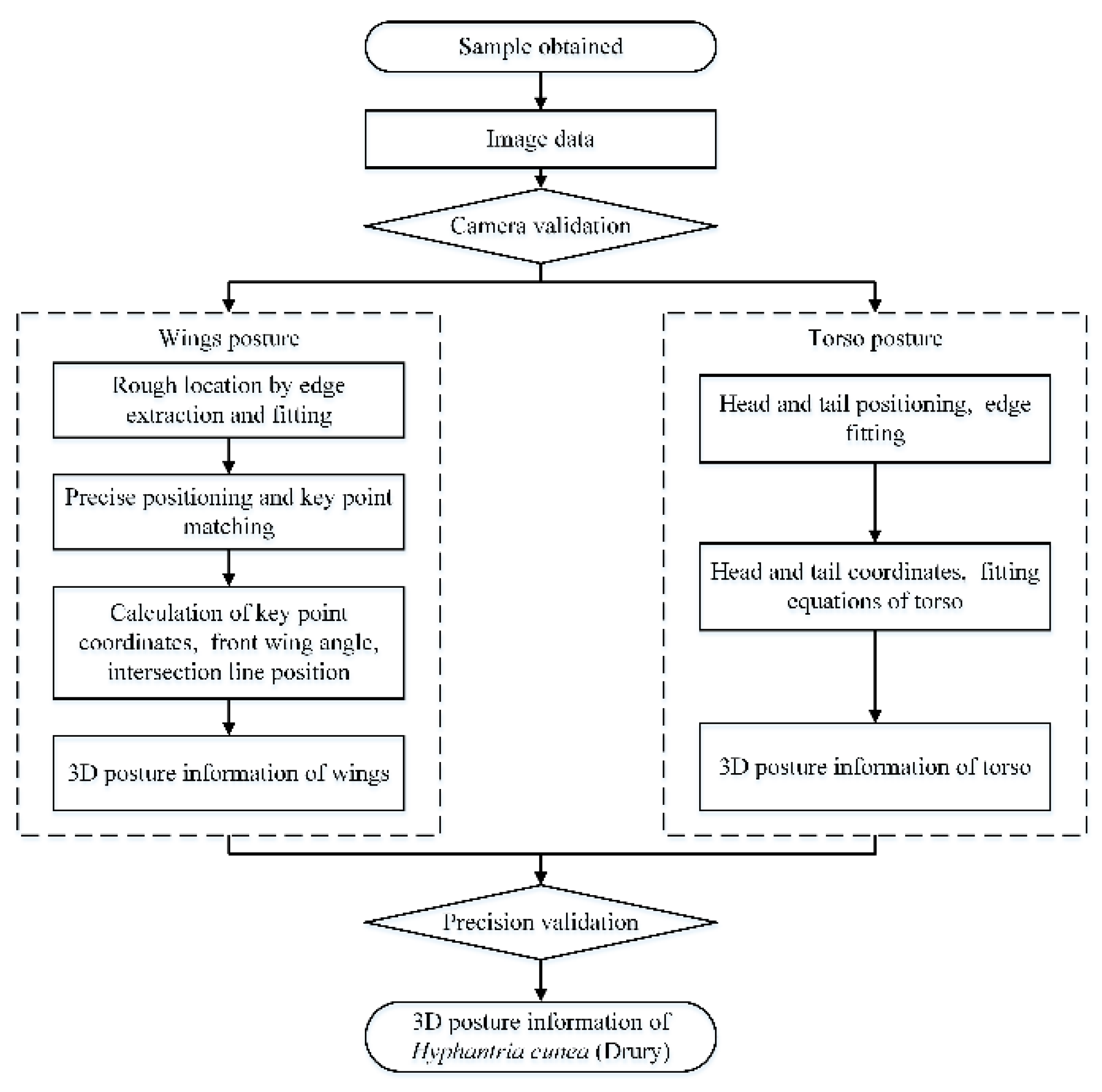
2.4.1. Overall Workflow

The image processing software used was MATLAB R2017a (Matrix Laboratory, Natick, MA, USA), the operating system was WIN10 (Microsoft, Seattle, WA, USA), the PC processor was Intel Core i7-7700, CPU 3.60 GHz. The extraction method of the 3D posture information of H. cunea was as follows:

• The characteristics of 3D posture change of multi-pose H. cunea were investigated, and the key feature points for extraction and localization methods of torso and wing posture information were determined.
• The 3D posture information of the H. cunea was extracted. The key points were located, the 3D coordinates of the key points were obtained, and the wing angle, the intersection equation of the wing plane, and the bending information of the torso were calculated. The calculation method of the torso and wing feature points was established to obtain the 3D information characteristics of H. cunea.
• A validation method for the accuracy of the 3D posture of H. cunea was established: a Metrology-grade 3D scanner (Artec Micro, Santa Clara, CA, USA) measurement method was used to verify the posture information obtained by monocular vision.

The entire extraction process is shown in Figure 5.

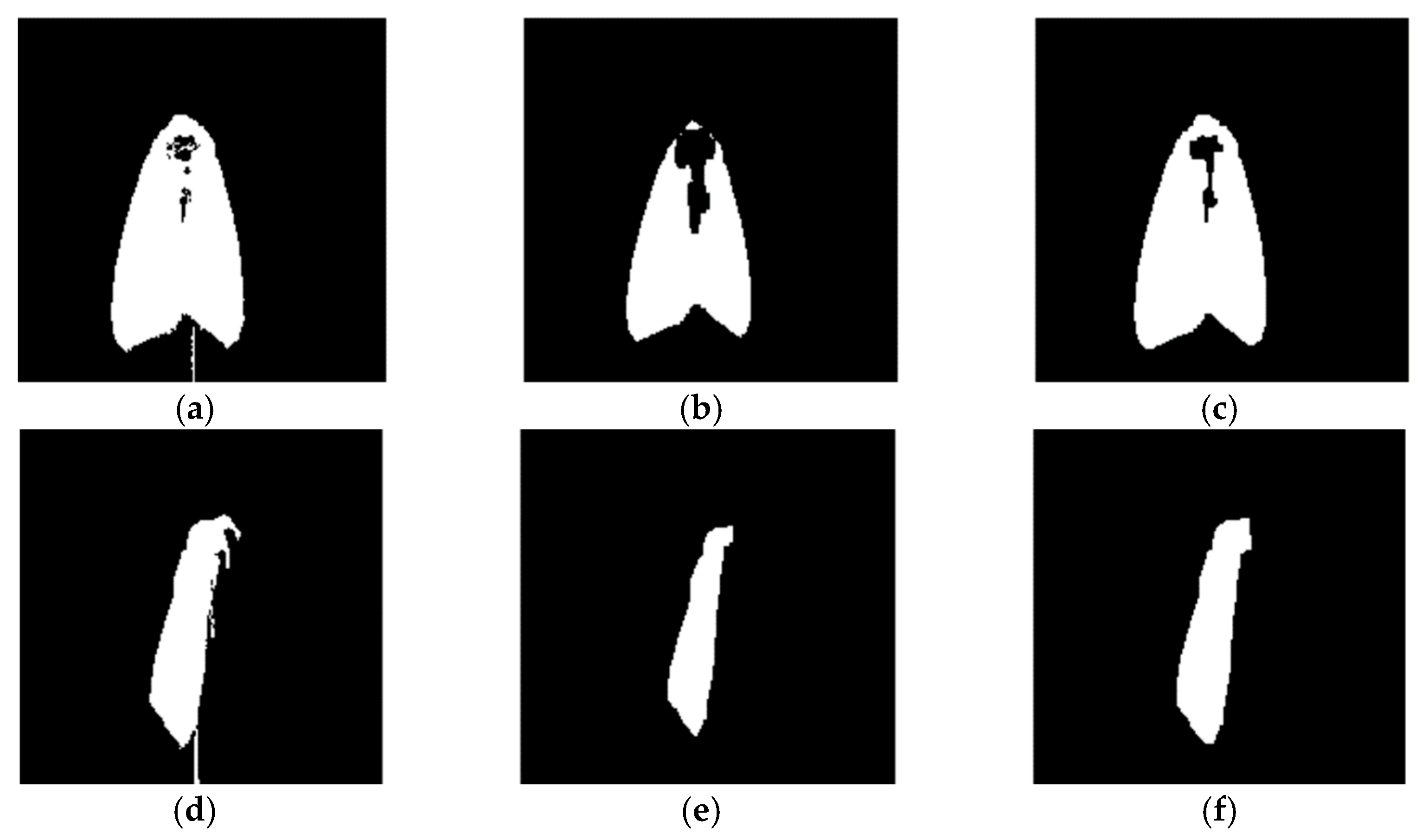
2.4.2. Image Preprocessing

The purpose of image preprocessing is to simultaneously extract the features of the target object and suppress the interference of non-target objects.

The color image of H. cunea was transformed to a gray image based on the rgb2gray() function. The speed of image processing was improved by removing the color information of the image while retaining the brightness information. In this study, median filtering was used to remove noise from the image, and to obtain edge information on H. cunea. Median filtering is a type of sequential statistical filtering suitable for extracting the edge of an image. The median filter function is expressed in Equation (1) [38].

$$B=medfilt2\left(A, \left[m,n\right]\right)$$

(1)

$A$ is the original image, $B$ is the processed image, $\left[m,n\right]$ is the two-dimensional template, $\left[m,n\right]$ is $3\times 3$ filter window by default.

Based on median filtering, the image was converted to a binary image through the application of erosion and dilation as shown in Figure 6. Then bwtraceboundary() function was used for edge tracking. All edge points were saved.

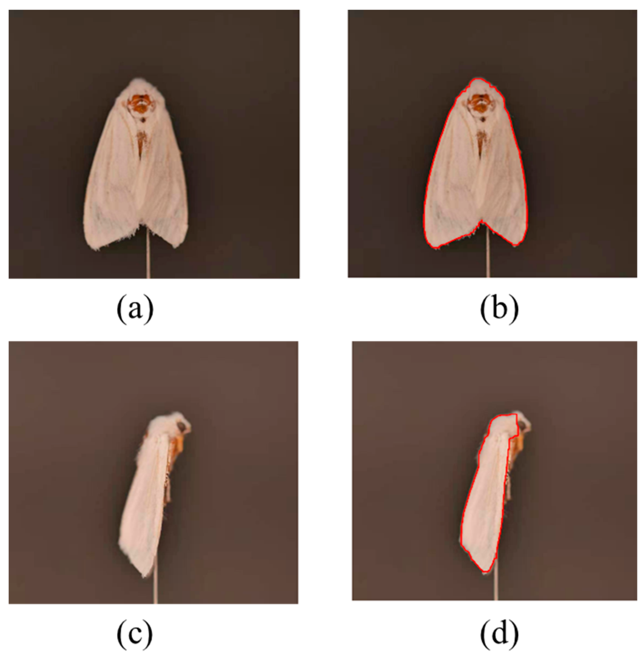
2.4.3. Approximate Location of Key Points

The target key points were the inflection points of the contour. The method in this study was to extract edge features, collect edge points, and synthesize the edge points into curves or straight lines. Then, the intersections of the lines were used as the reference points for the key points. The key point was located near the reference point, but the key point must be located precisely.

The specific experimental scheme was as follows. According to the posture characteristics of H. cunea, the 3D posture characteristics of its wing were divided into two types. In the first case, the wings of the H. cunea were withdrawn, and the angle of the wings was less than 180°. First, the images of H. cunea were preprocessed to provide a basis for subsequent detection and localization. As shown in Figure 6, the image was converted to a binary image, and erosion and dilation were used to eliminate the influence of insect needles and other non-wing contours. Then the bwtraceboundary() function was used for edge tracking, given the search starting point and search direction. The function returned a line coordinate array. Figure 7 shows the edge tracking result. The coordinate points after tracking and extraction were saved as an Excel table.

The second step was edge fitting. There were too many edge points stored from each picture, which would not improve the fitting accuracy and would increase the fitting time. Thus, a step size of 10 was set for the edge points, and the coordinates of one point every step distance were saved. Then, n_i edge points could be screened out for edge fitting.

When the wings angle of the H. cunea was less than 180°, points of the anal angle of the two wings overlapped. For the dorsal image, according to the location of five reference points of the humeral, apical, anal angle, the n_i points must be divided into five sections, and the five reference points must be fitted. The edge points were segmented by traversing all of them. The maximum and minimum points of x and y in the coordinates (x,y) were selected; that is, four points on edge, A1, A2, and A4. The points larger than the ordinate of the left and right adjacent points were selected as A3 and A9, respectively. Points A5 and A6 were selected according to (l_A1–A3)/(l_A1–A5) = 5, and (l_A1–A9)/(l_A1–A6) = 5. The point A8 with the lowest y-coordinate was selected after traversing l_A3–A9. Finally, A5, A6, A3, A8, and A9 were used as the segmentation points, and the images in Figure 8 were obtained after edge fitting. The intersection of the two fitting lines was denoted as the reference point of the key point. Similarly, the n_i points of the right-side view image rotated 90° clockwise should be divided into 4 sections, and 3 key points could be obtained by fitting the curve. The minimum points of x, maximum and minimum points of y in the coordinates (x,y) of the right view image were selected, that is, the three most marginal points B1, B2, and B3. Points B4 and B5 were selected according to (l_B1–B3)/(l_B1–B5) = 5, and (l_B1–B2)/(l_B1–B4) = 5. B2, B3, B4, and B5 were used as the segmentation points, and the image in Figure 8d was obtained after edge fitting. The intersection of the two fitting lines was denoted as the reference point of the key point.

In the second case. with the wings of H. cunea unfolded, the angle of the wings was more than 180°, and there was no triangle contour from the dorsal view image. The right and left view images were obtained when the H. cunea rotated 90°, and the approximate triangular wings were clearly visible. The outline of the humeral angle point was calculated based on the above methods, and key points were approximately positioned after fitting right and left view image edge points. The anal angle point was the lowest point in the wing profile, that is, the point with the lowest y value. The apical corner of the right wing is the leftmost point of the contour points, that is, the lowest x value point. The apical corner of the left wing is the rightmost point of the contour points, that is, the point with the maximum x value. The apical corner of the left wing was the rightmost point of the contour points, that is, the point with the maximum x value. Figure 9 shows the left-wing humeral angle fitting schematic diagram and the right-wing humeral angle fitting contraction.

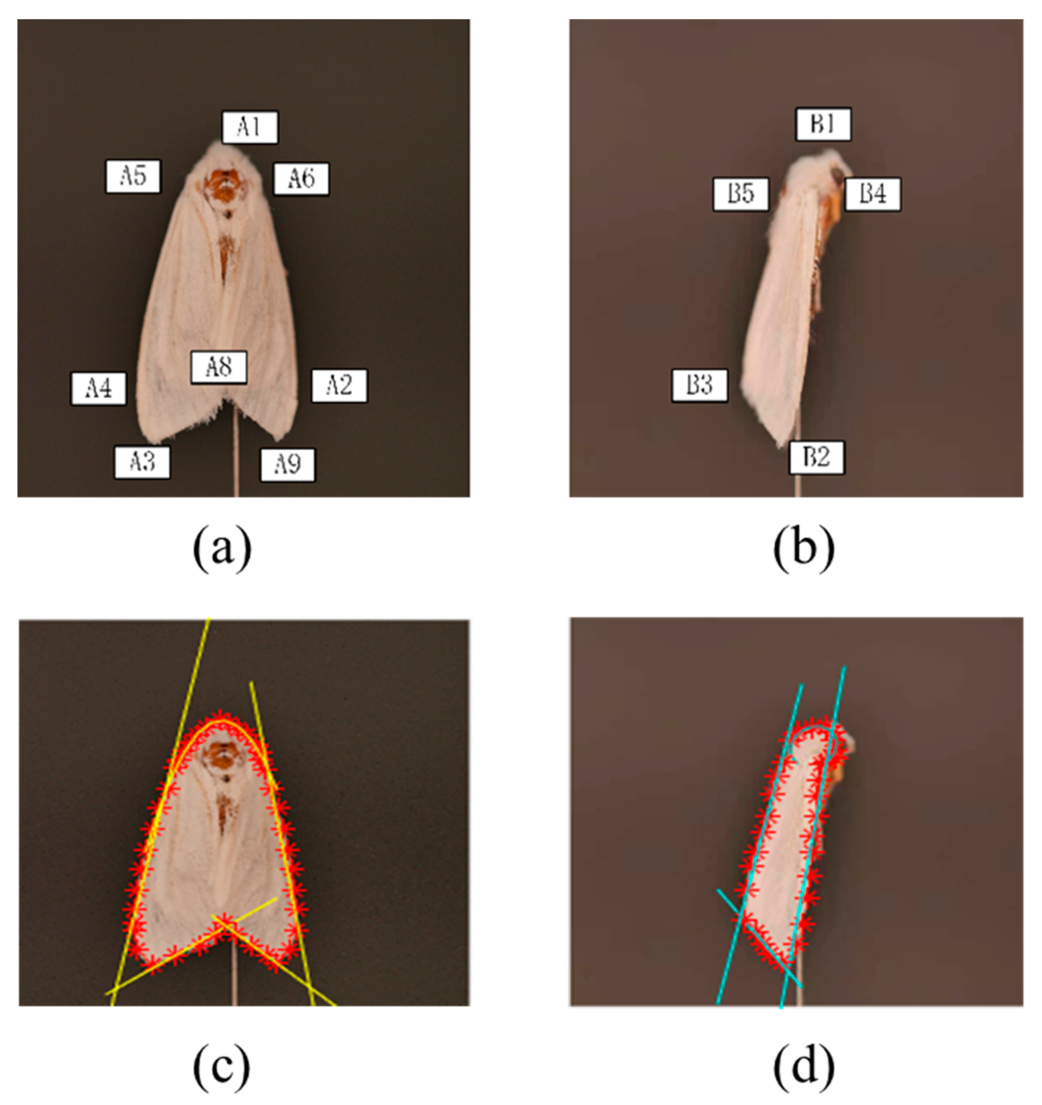
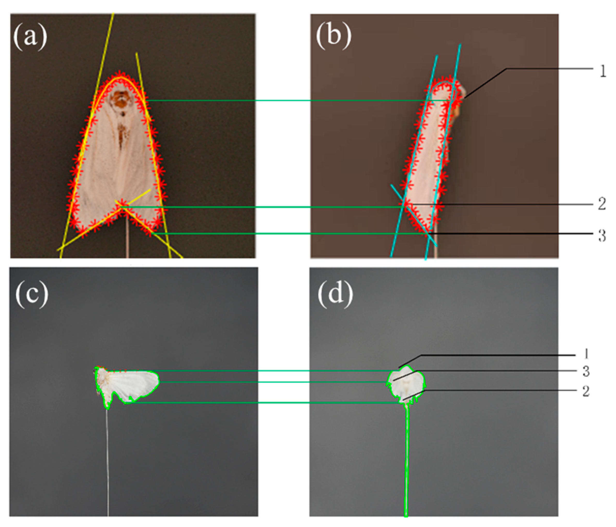
2.4.4. Precise Positioning and Matching of Key Points

The precise method consisted of calculating the reference points of the humeral, apical, and anal angle points on each wing. Then, the 10 points closest to the reference point in all edge points were traversed, and the center point of the 10 points was calculated; that is, the precise coordinates of the key points were obtained according to the following Equation (2).

$$X={\displaystyle \sum }_{i=1}^{10}{x}_{i, }Y={\displaystyle \sum }_{i=1}^{10}{y}_i$$

(2)

where $X$ and $Y$ are the coordinates of center point on X and Y axes respectively. $x_i$, and $y_i$ are the coordinates of edge points on X and Y axes. Since the camera was fixed when taking the image, a picture was taken when the insect needle rotated 90° clockwise. Therefore, the abscissa of the key points changed, but the ordinate remained the same (i.e., the y values of the two matched key points were the same). Owing to the error in finding the intersection point of the fitting edge, the coordinate y of the corresponding key points of the two pictures may not be equal. The two y values were averaged to obtain the final y value of the key points on the dorsal right side. Finally, the coordinates (x_l1,y_l1), (x_bl1,y_l1) and (x_br1,y_r1), (x_r1,y_r1) of two pairs of humeral angle points, the coordinates (x_l2,y_l2), (x_bl2,y_l2) and (x_br2,y_r2), (x_r2,y_r2) of two pairs of anal angle points, and the coordinates (x_l3,y_l3), (x_bl3,y_l3) and (x_br3,y_r3), (x_r3,y_r3) of two pairs of apical angle points were obtained.

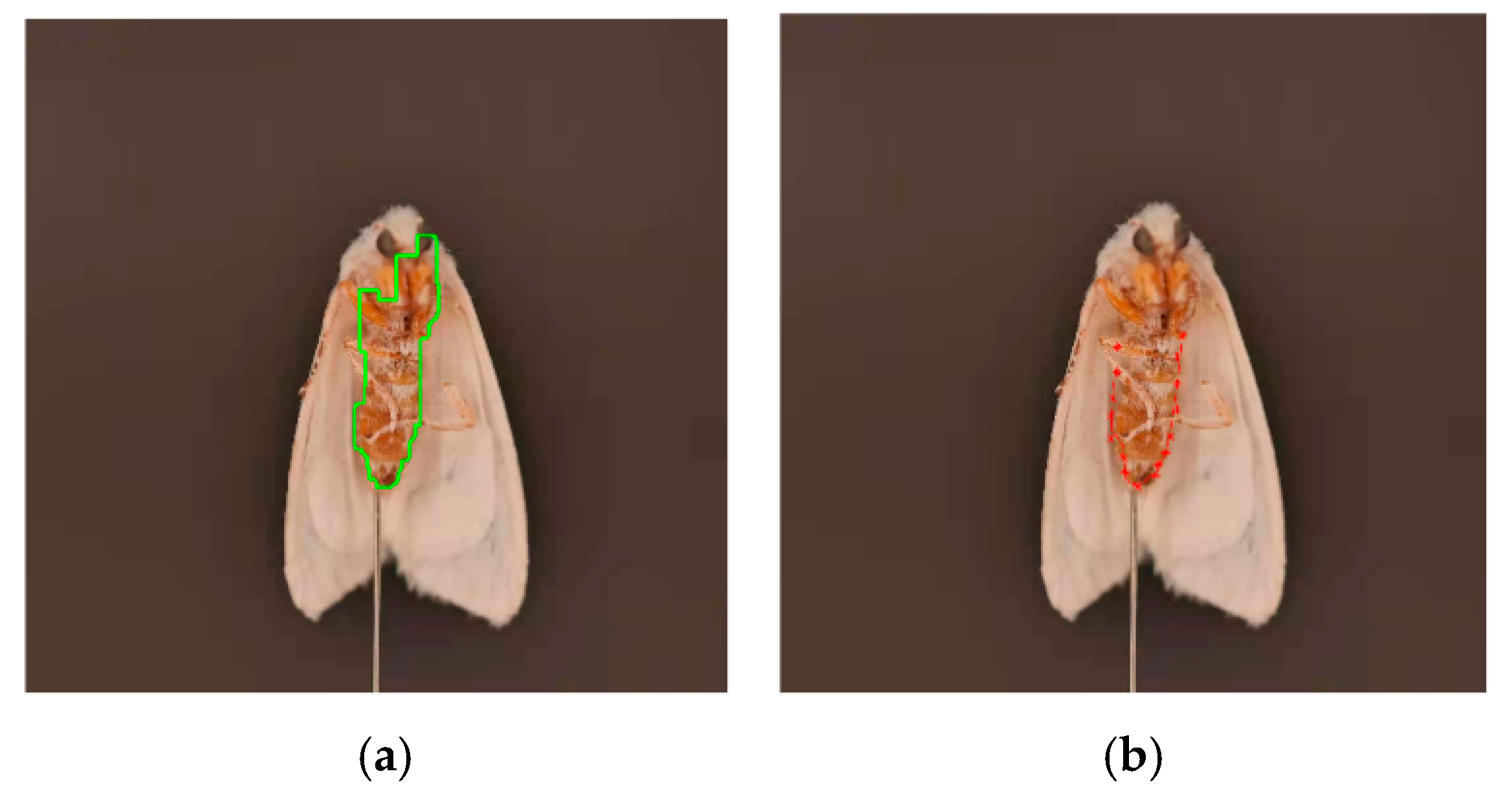
2.4.5. Extraction of 3D Posture Features of the Torso

If the angle of the wings of the H. cunea was greater than 180°, its abdomen was visible. The abdominal image was obtained when H. cunea was rotated 180° from the dorsal view, and another image was obtained when H. cunea was rotated 90° again. Curve contour fitting was performed in the middle, as shown in Figure 10. Finally, two points and four curve segments were combined to form a 3D frame.

If the angle of the wings was less than 180°, the abdomen was not completely visible, and half of it was covered by wings. In this case, the abdomen image could not be collected unless the wings of the insect were removed. Twenty H. cunea samples with the angle of the wings smaller than 180° were found, and their wings were removed to expose their abdomens. Two view pictures were obtained, and the proportion of the width of the same ordinate value between the part covered by the wing and the part not covered by the wing was calculated. Because the partial error of the abdominal occlusion had little influence on the experimental results, the 3D posture information of the edge position and bending of the occluded part of the H. cunea could be calculated from the side that was not occluded.

2.4.6. Calculation of the 3D Posture Information

The 3D posture information of wings of H. cunea included two pairs of coordinates for the humeral angle point (x_l1,y_l1), (x_bl1,y_l1) and (x_br1,y_r1), (x_r1,y_r1), two pairs of coordinates for the anal angle point (x_l2,y_l2), (x_bl2,y_l2) and (x_br2,y_r2), (x_r2,y_r2), and two pairs of coordinates for the apical angle point (x_l3,y_l3), (x_bl3,y_l3) and (x_br3,y_r3), (x_r3,y_r3). Then, the 3D coordinates of every key point could be obtained.

The position of H. cunea in space is shown in Figure 11, and the coordinate system was established, as shown in Figure 12.

The relationship between 2D point coordinates and 3D point coordinates was obtained as follows.

Right wing:

$$\{\begin{array}{c}{x}_r=-\left(x_{-}r-X_r\right)=X_r-x_{-}r\\ y_r=x_{-}br-Y\\ z_r=y,\end{array}$$

(3)

and left wing:

$$\{\begin{array}{c}{x}_l=x_{-}l-X_l\\ y_l=x_{-}bl-Y\\ z_l=y.\end{array}$$

(4)

In the formula, X_r is the abscissa of the insect needle on the right-wing diagram, X_l is the abscissa of the insect needle on the left-wing diagram, Y is the abscissa of the insect needle in the dorsal view, x_r is the 2D abscissa of the center point of the right-side view image, x_l is the 2D abscissa of the center point of the left-side view image, x_br is the 2D abscissa of a point on the right wing in a dorsal view image, x_bl is the 2D abscissa of a point on the left wing in a dorsal view image, and y is the corresponding average ordinate of the two viewing angles.

According to Equations (3) and (4), the 3D coordinates of each key point and two sets of coordinates or six coordinate points of the H. cunea sample were obtained. Then, the plane of each wing, according to the three points, the plane normal vector, and the angle between the two planes could be calculated, that is, the angle between the two wings. The two plane equations were simultaneous, and the equation of the intersection line and its direction vector was obtained.

The establishment of the coordinate system and the conversion formula of the 2D and 3D coordinate systems of the torso were the same as those of the wing. Finally, four 3D curve equations and the 3D coordinates of the head and tail were obtained; this was the 3D posture information of the torso.

2.5. Accuracy Verification of the 3D Information Extraction

To verify the feasibility and reliability of the proposed method, the results of the study were compared with the reference values of a Metrology-grade 3D scanner measurement. The reference values of the angles between the wings of the H. cunea were measured by a Metrology-grade 3D scanner with a point accuracy of up to 10 microns. The two methods were compared to verify the reliability of the method proposed for the extraction of 3D posture information of H. cunea in this study.

Paired samples refer to the same samples tested twice at different times or to two samples that had similar test records. The differences between paired samples were compared. In this study, every method was tested twice on each H. cunea sample. Therefore, the data of the two methods could be paired, meeting the conditions of a paired t-test for their comparison. To verify the accuracy of the proposed method and measure the calculation deviation, the root mean square error (RMSE) was calculated: the smaller the error, the higher the accuracy.

During the extraction and verification of the 3D abdominal information of H. cunea, for each fitting equation, a number of points were found along its corresponding abdominal edge at a certain distance. A Metrology-grade 3D scanner was used to measure the points and find their coordinates. When x = 0, y was put into the equation for the torso, and z₁ was obtained. When y = 0, x was put into the equation, and z₁ was obtained. Then z₁ was compared with the coordinate z measured by the Metrology-grade 3D scanner.

3. Results and Discussion

3.1. Result

In the study, four images were taken for each H. cunea sample for a total of nine samples, and 36 images were obtained. In Figure 13, matching results of key points for different angles of the wings were presented. As shown in Figure 13, the key points of wings with different angles were well identified, and the corresponding fit lines were of a reasonable accuracy.

The angle between the wings and the direction vector of the intersection line for each sample was calculated, as shown in

Table 1. Angle between the wings and the direction vector of intersecting lines for each sample.

Sample	Angle between the Wings (°)	Direction Vector of Intersecting Lines
1	103.3151	1 × 1010 × (−0.3349, −0.0415, −1.6122)
2	286.5005	1 × 109 × (1.0672, −0.1245, 0.8172)
3	127.7247	1 × 1011 × (0.0041, 0.0049, −1.1289)
4	102.4134	1 × 1011 × (0.2565, 0.0142, 1.2537)
5	72.4769	1 × 1010 × (−0.5009, 0.2267, 7.0706)
6	150.6711	1 × 1010 × (−2.7502, 0.1524, −5.3349)
7	342.7297	1 × 1010 × (−4.5790, −0.3979, −4.2846)
8	172.2616	1 × 1010 × (0.0630, 2.3785, −6.0611)
9	271.8351	1 × 1010 × (0.9570, 2.2869, 9.5959)

. In Table 1, it can be seen that different samples have the variant angle of the wings; for example, 72.4769° for sample 5, while 342.7297 for sample 7. Specifically, the direction vectors of intersecting lines were also presented in Table 1. As shown in Table 1, the direction vectors of intersecting lines were slightly different for different angles between the wings, even for similar angles of wings; for example, in sample 1 and sample 4, the angles of wings are 103.3151, and 102.4134, but the direction vectors of intersecting lines are also quite different. This means the diversity and complexity of H. cunea in the real world.

The contour features of H. cunea were extracted, as shown in

Table 2. 3D torso information of the samples, including 3D coordinates of head and tail, and corresponding fitted equation. The 3D coordinates of the head and tail are presented in image coordinates.

Sample	Head Coordinates	Tail Coordinates	Fitting Equation of Torso Edge
1	(−50, −20, 280)	(0, 0, 752)	z = −0.0013y3 + 0.867y2 − 2.4018y + 764.8990 z = −0.0398y3 − 1.5512y2 − 1.9434y + 855.0992 z = −0.0013x3 + 0.867x2 − 2.4018x + 764.8990 z = −0.0398x3 − 1.5512x2 − 1.9434x + 855.0992
2	(0, 0, 322)	(0, 0, 632)	z = −0.0226 × x2 + (−1.1978 × x) + 661.8303 z = −0.1110 × x2 + (2.4081× x) + 645.0075 z = −0.0110 × y2 + (−3.5920 × y) + 668.6825 z = −0.1332 × y2 + (−3.1020 × y) + 652.3501
3	(34, −23, 194)	(0, 0, 487)	z = 0.0007 × y3 + (−0.1996 × y2) + (−6.9745 × y) + 433.1011 z = 0.0024 × y3 + (−0.2119 × y2) + (−0.5866 × y) + 498.5497 z = 0.0007 × x3 + (−0.1996 × x2) + (−6.9745 × x) + 433.1011 z = 0.0024 × x3 + (−0.2119 × x2) + (−0.5866 × x) + 498.5497
4	(24, −43, 180)	(0, −21, 479)	z = −0.0001 × y3 + (−0.0185 × y2) + (−0.5754 × y) + 516.1118 z = −0.0381 × y3 + (0.9691 × y2) + (2.1505 × y) + 372.4526 z = −0.0001 × x3 + (−0.0185 × x2) + (−0.5754 × x) + 516.1118 z = −0.0381 × x3 + (0.9691 × x2) + (2.1505 × x) + 372.4526
5	(0, 0, 380)	(0, −10, 491)	z = −0.7636 × y3 + (65.3431 × y2) + (−1842.6824 × y) + 17,521.4701 z = 0.0013 × y3 + (0.0429 × y2) + (0.4754×y) + 482.8186 z = −0.7636 × x3 + (65.3431 × x2) + (−1842.6824 × x) + 17,521.4701 z = 0.0013 × x3 + (0.0429 × x2) + (0.4754 × x) + 482.8186
6	(−220, 0, 980)	(0, 35, 1730)	z = 0.0001 × y3 + (−0.0176 × y2) + (−1.6880 × y) + 1753.9989 z = 0.0730 × y3 + (12.3106 × y2) + (675.1220 × y) + 13,564.7679 z = 0.0001 × x3 + (−0.0176 × x2) + (−1.6880 × x) + 1753.9989 z = 0.0730 × x3 + (12.3106 × x2) + (675.1220 × x) + 13,564.7679
7	(−130, 40, 1300)	(0, −30, 1990)	z = −0.3541 × y2 + (38.6749 × y) + 1014.3517 z = −0.0397 × y2 + (1.6088 × y) + 1984.9320 z = 0.1512 × x2 + (−33.5388 × x) + 3533.1131 z = −0.2801 × y2 + (−32.5045 × y) + 993.5104
8	(0, 0, 1030)	(0, 0, 1852)	z = −0.0844 × y2 + (2.2203 × y) + 1814.2713 z = −0.0145 × y2 + (0.6312 × y) + 1893.2772 z = −0.0844 × x2 + (2.2203 × x) + 1814.2713 z = −0.0145 × x2 + (0.6312 × x) + 1893.2772
9	(80, −80, 700)	(0, 41, 1616)	z = −0.0281 × y2 + (−0.5978 × y) + 1605.8748 z = −0.0486 × y2 + (−0.9896 × y) + 1660.7973 z = −0.0281 × x2 + (−0.5978 × x) + 1605.8748 z = −0.0486 × x2 + (−0.9896 × x) + 1660.7973

. The point with the smallest ordinate of the pixel was the head, and the point with the largest ordinate of the pixel was the tail. The curve contour of H. cunea abdomen was also fitted and showed in Table 2.

3.2. Accuracy Verification

The angle results of H. cunea wings obtained in this study were compared with the reference values measured by the Metrology-grade 3D scanner. The comparison results are shown in

Table 3. Accuracy validation of study, the result from 3D scanner is used as truth data. The measured, reference value, the absolute and relative errors are shown for each sample.

Samples	Measured Value (°)	Reference Value (°)	Absolute Error (°)	Relative Tolerance (%)
1	103.3151	106.5433	−3.2282	3.03
2	286.5005	287.4093	−0.9088	0.32
3	127.7247	129.6543	−1.9296	1.49
4	102.4134	104.6035	−2.1901	2.09
5	72.4769	73.7544	−1.2775	1.73
6	150.6711	152.9886	−2.3175	1.51
7	342.7297	340.9005	1.8292	0.54
8	172.2616	173.5770	−1.3154	0.76
9	271.8351	270.4576	1.3775	0.51

. Comparing the Metrology-grade 3D scanner measurement results with the results obtained by the proposed method, the relative error range was from 0.32% to 3.03%, and the average relative error was 1.33%, both within the range of (100% ± 5%). According to the statistical principle, the data results were reliable [39].

In this study, the wing angle calculation method and the Metrology-grade 3D scanner measurement calculation method were matched using a t-test. The inspection results of t between the reference and measured value of the angle of the wings of H. cunea are shown in

Table 4. t-test between reference and measured values of the angle of the wings angle of H. cunea samples.

Item	Mean (°)	Standard Deviation (°)	t Value	df	Sig. (Two-Sided)
Reference and Measured Values	−1.1067	1.6852	−1.970	8	0.084

(p = 0.084, which is greater than the statistical significance, which was set at 0.05). Thus, there was no significant difference between the reference value and the measured value of the wing angle, and the results showed that this method was sufficiently accurate.

To test the accuracy of the proposed calculation method, we determined the calculation deviation and calculated the RMSE (also known as standard error). The RMSE was 1.9363°, which showed that the error between reference and measured values was small, the accuracy of this method was high.

For the verification of the 3D torso information, six points were selected from one equation. The verification results are shown in

Table 5. Verification result of the H. cunea sample. The truth value (measured value) and the calculated value of coordinate Z are presented in pixel, and the absolute and relative errors are calculated.

The Selected Marker Point	Measured Value of Coordinate Z (pixel)	Calculated Value of Coordinate Z (px)	Absolute Error	Relative Tolerance
1	386	404	18	4.66
2	397	421	24	6.04
3	424	427	3	0.71
4	452	460	8	1.77
5	540	552	12	2.22
6	564	571	7	1.24

. The maximum relative error was 6.04%, the minimum relative error was 0.71%, and the average relative error was 2.77%. The results obtained by other fitting equations were consistent with Table 5. Therefore, using this method, there were large errors in individual areas, but the overall abdominal contour could be approximately defined by the fitting equation.

3.3. Discussion

The research on using monocular vision to calculate the 3D pose information of H. cunea is less reported. Currently, 3D scanner measurement is the most accurate method to obtain the 3D pose information of H. cunea. However, the high cost of the device limits the wide usage of this method. In this study, a low-cost device was constructed, and the corresponding algorithm was developed to calculate the 3D pose information of H. cunea. The accuracy validation shown in Section 3 indicates the performance of the presented method achieved a reasonable accuracy. The average relative error of measured angles of wings was 1.33% for the presented method when compared to the true value from the 3D scanner. This error is similar to the angle measurement of wings conducted by another research, for example, 1.02% for Bollworm [36]. Thus, the present method can be used to obtain 3D pose information of H. cunea in a cheap and fast way. As a result, the application of machine vision and deep learning in pest recognition may benefit from the study, for the training samples can be obtained more easily than before.

The result shown in Table 3 indicates that the absolute errors vary with individuals, and the relative errors were range from 0.32% to 3.03%. This means the performance of the method may be influenced by the input samples. In fact, for monocular vision, the depth, as well as clarity of images are both important in this study [40,41]. In some cases, we could not obtain an image with both depth and clarity well. As a result, the inaccurate input images decrease the performance of the method. As for the presented method, inaccurate input images influence the estimation accuracy of the torso, including the three aspects. Firstly, an unclear image would decrease the accuracy of the key points obtained from the feature extraction method. Then, the low-quality key points influence the matched key points. As a result, it decreased the accuracy of the fitted edge and obtained inaccurate angles of the wings or 3D torso information. Thus, more work needs to be conducted on how to improve the quality of the captured images and enhance the robustness of the method.

4. Conclusions

H. cunea was selected as the representative moth for this experiment, which aimed to create and verify an algorithm to extract 3D posture. Feature point extraction and location method of posture information of H. cunea wing and torso was developed, and the 3D information of H. cunea was obtained. The accuracy of the 3D posture information was verified, and the results showed that the 3D information of H. cunea was obtained accurately by this method. The 3D posture information could provide a data source for 3D model deformation simulation. To conclude this paper, the following key points are summarized about the extraction and location method of 3D posture information of H. cunea.

The images of H. cunea were obtained by an insect image acquisition system, and the posture change of the moth included wing and torso deformation. The wing deformation is caused by the rotation of the wing around the humeral angle, and the torso deformation is caused by bending and twisting of the torso. According to the characteristics of the posture change of the moth, the 3D posture of H. cunea was defined, and the key parts that could represent the 3D posture information of H. cunea were determined.

The approximate location of the insect wing key points was established based on boundary tracking and edge fitting. The coordinates of the key points of the wings were obtained based on precise location and key-point matching. The angle of the wings was calculated to obtain the 3D posture information of the wings. The 3D posture information of H. cunea wing angle obtained by this method was compared with the Metrology-grade 3D scanner measurement, and the results showed that the relative error of the wing angle was between 0.32% and 3.03%, the average relative error was 1.33%, and the RMSE was 1.9363.

Through the edge extraction and curve fitting of the abdomen, the head and tail coordinates and the fitting equations of the torso edge of H. cunea were obtained to extract the 3D posture of the insect abdomen. The information obtained by this method was compared with the Metrology-grade 3D scanner measurements, and the results showed that the average relative error of the torso was 2.77%.

The above results confirmed that the proposed method for extraction of 3D posture information of H. cunea was accurate. The 3D posture information of H. cunea extracted using our method can provide important data support for sample augmentation and species identification of moth pests.

References

1. Liu, H.J.; Luo, Y.Q.; Wen, J.B.; Zhang, Z.M.; Feng, J.H.; Tao, W.Q. Pest risk assessment of Dendroctonus valens, Hyphantria cunea and Apriona swainsoni in Beijing area. J. Beijing For. Univ. 2005, 27, 81–87. [Google Scholar]
2. Wen, C.; Wu, D.; Hu, H.; Wei, P. Pose estimation-dependent identification method for field moth images using deep learning architecture. Biosyst. Eng. 2015, 136, 117–128. [Google Scholar] [CrossRef]
3. Lv, J.; Yao, Q.; Liu, Q.; Xue, J.; Chen, H.M.; Yang, B.J.; Tang, J. Multi-target rice lamp trap pest identification based on template matching Method research. China Rice Sci. 2012, 26, 619–623. [Google Scholar]
4. Li, W.Y.; Chen, M.X.; Li, M.; Sun, C.H.; Du, S.F. Automatic identification method of target pests in orchard based on attitude description. Agric. Chin. J. Mech. Eng. 2014, 45, 54–59. [Google Scholar] [CrossRef]
5. Li, W.Y.; Du, S.F.; Li, M.; Chen, M.X.; Sun, C.H. Fuzzy classification of orchard pest posture based on Zernike moments. In Proceedings of the IEEE International Conference on Fuzzy Systems (FUZZ-IEEE), Beijing, China, 6–11 July 2014. [Google Scholar]
6. Li, W.Y.; Li, M.; Chen, M.X.; Qian, J.P.; Sun, C.H.; Du, S.F. Feature extraction and multi-pose pests of crops based on machine vision Classification method. Trans. Chin. Soc. Agric. Eng. 2014, 30, 154–162. [Google Scholar]
7. Ding, W.G.; Taylor, G. Automatic moth detection from trap images for pest management. Comput. Electron. Agric. 2016, 123, 17–28. [Google Scholar] [CrossRef] [Green Version]
8. Chen, J.; Fan, Y.Y.; Wang, T.; Zhang, C.; Qiu, Z.J.; He, Y. Automatic Segmentation and Counting of Aphid Nymphs on Leaves Using Convolutional Neural Networks. Agronomy 2018, 8, 129. [Google Scholar] [CrossRef] [Green Version]
9. Cheng, X.; Zhang, Y.; Chen, Y.; Wu, Y.; Yue, Y. Pest identification via deep residual learning in complex background. Comput. Electron. Agric. 2017, 141, 351–356. [Google Scholar] [CrossRef]
10. Xie, C.; Wang, R.; Zhang, J.; Chen, P.; Dong, W.; Li, R.; Chen, T.; Chen, H. Multi-level learning features for automatic classification of field crop pests. Comput. Electron. Agric. 2018, 152, 233–241. [Google Scholar] [CrossRef]
11. Shen, Y.; Zhou, H.; Li, J.; Jian, F.; Jayas, D.S. Detection of stored-grain insects using deep learning. Comput. Electron. Agric. 2018, 145, 319–325. [Google Scholar] [CrossRef]
12. Sun, Y.; Zhang, D.Y.; Yuan, M.S.; Ren, L.L.; Liu, W.P.; Wang, J.X. In-trap red turpentine beetle detection model based on deep learning. Agric. Chin. J. Mech. Eng. 2018, 49, 180–187. [Google Scholar]
13. He, Y.; Zhou, Z.Y.; Tian, L.H.; Liu, Y.F.; Luo, X.W. Brown rice planthopper (Nilaparvata lugens Stal.) detection based on deep learning. Precis. Agric. 2020, 21, 1385–1402. [Google Scholar] [CrossRef]
14. Wang, F.Y.; Wang, R.J.; Xie, C.J.; Yang, P.; Liu, L. Fusing multi-scale context-aware information representation for automatic in-field pest detection and recognition. Comput. Electron. Agric. 2020, 169, 11. [Google Scholar] [CrossRef]
15. Jiao, L.; Dong, S.F.; Zhang, S.Y.; Xie, C.J.; Wang, H.Q. AF-RCNN: An anchor-free convolutional neural network for multi-categories agricultural pest detection. Comput. Electron. Agric. 2020, 174, 9. [Google Scholar] [CrossRef]
16. Khanramaki, M.; Askari, A.E.; Kozegar, E. Citrus pests classification using an ensemble of deep learning models. Comput. Electron. Agric. 2021, 186, 11. [Google Scholar] [CrossRef]
17. Wang, K.; Mu, Z.C. A 3D ear recognition method with pose robustens. China Sci. Pap. 2013, 8, 6. [Google Scholar]
18. Tang, H.L. Face Recognition Based on 3D Features. Ph.D. Dissertation, Beijing University of Technology, Beijing, China, 2011. [Google Scholar]
19. Bel, B.S.; Schmelzle, S.; Blüthgen, N.; Heethoff, M. An automated device for the digitization and 3D modelling of insects, combining extended-depth-of-field and all-side multi-view imaging. ZooKeys 2018, 759, 1–27. [Google Scholar]
20. Lau, J.M. 3D digital model reconstruction of insects from a single pair of stereoscopic images. J. Microsc.-Oxford 2013, 212, 107–121. [Google Scholar]
21. Nguyen, C.; Lovell, D.; Oberprieler, R.; Jennings, D.; Adcock, M.; Gates-Stuart, E.; Salle, J. Virtual 3D Models of Insects for Accelerated Quarantine Control. In Proceedings of the IEEE International Conference on Computer Vision (ICCV) Workshops, Sydney, NSW, Australia, 2–8 December 2013; pp. 161–167. [Google Scholar]
22. Nguyen, C.V.; Lovell, D.R.; Adcock, M.; La, S.J. Capturing natural-colour 3D models of insects for species discovery and diagnostics. PLoS ONE 2014, 9, e94346. [Google Scholar] [CrossRef] [PubMed] [Green Version]
23. Qian, J.; Dang, S.; Wang, Z.; Zhou, X.; Dan, D.; Yao, B.; Tong, Y.; Yang, H.; Lu, Y.; Chen, Y.; et al. Large-scale 3D imaging of insects with natural color. Opt. Express 2019, 27, 4845–4857. [Google Scholar] [CrossRef] [PubMed]
24. Ge, S.Q.; Wipfler, B.; Pohl, H.; Hua, Y.; Slipiński, A.; Yang, X.K.; Beutel, R.G. The first complete 3D reconstruction of a Spanish fly primary larva (Lytta vesicatoria, Meloidae, Coleoptera). PLoS ONE 2012, 7, e52511. [Google Scholar] [CrossRef] [PubMed]
25. Ge, S.Q.; Hua, Y.; Ren, J.; Slipinski, A.; Wipfler, B. Transformation of head structures during the metamorphosis of Chrysomela populi (Coleoptera: Chrysomelidae). Arthropod Syst. Phylogeny 2015, 73, 129–152. [Google Scholar]
26. Grzywacz, A.; Goral, T.; Szpila, K.; Hall, M.J.R. Confocal laser scanning microscopy as a valuable tool in Diptera larval morphology studies. Parasitol. Res. 2014, 113, 4297–4302. [Google Scholar] [CrossRef] [PubMed] [Green Version]
27. Klaus, A.V.; Kulasekera, V.L.; Schawaroch, V. Three-dimensional visualization of insect morphology using confocal laser scanning microscopy. J. Microsc.-Oxford 2003, 212, 107–121. [Google Scholar] [CrossRef] [PubMed]
28. Li, W.P. Three-Dimensional Live Monitoring of Insect Embryo Development and Microcirculation Imaging Based on OCT Technology. Master’s Thesis, Hebei University, Baoding, China, 2018. [Google Scholar]
29. Mohoric, A.; Bozic, J.; Mrak, P.; Tusar, K.; Lin, C.; Sepe, A.; Mikac, U.; Mikhaylov, G.; Sersa, I. In vivo continuous three-dimensional magnetic resonance microscopy: A study of metamorphosis in Carniolan worker honey bees (Apis mellifera carnica). J. Exp. Biol. 2020, 223, jeb225250. [Google Scholar] [CrossRef] [PubMed]
30. Rother, L.; Kraft, N.; Smith, D.B.; El Jundi, B.; Gill, R.J.; Pfeiffer, K. A micro-CT-based standard brain atlas of the bumblebee. Cell Tissue Res. 2021, 386, 29–45. [Google Scholar] [CrossRef] [PubMed]
31. Yu, X.; Sun, M. A computational study of the wing–wing and wing–body interactions of a model insect. Acta Mech. Sin. 2009, 25, 421–431. [Google Scholar] [CrossRef]
32. Chen, M.W.; Sun, M. Experimental observation and mechanical analysis of the rapid take-off process of bees and flies. Acta Mech. Sin. 2014, 35, 3222–3231. [Google Scholar]
33. Chen, M.W.; Zhang, Y.L.; Sun, M. Wing and body motion and aerodynamic and leg forces during take-off in droneflies. J. R. Soc. Interface 2013, 10, 20130808. [Google Scholar] [CrossRef] [Green Version]
34. Huang, Y.B. Motion Analysis and Simulation Design of Flapping Wing Flight. Master’s Thesis, Zhejiang University, Hangzhou, China, 2018. [Google Scholar]
35. Lv, D.; Sun, J.F.; Li, Q.; Wang, Q. 3D pose estimation of target based on ladar range image. Infrared Laser Eng. 2015, 44, 1115–1120. [Google Scholar]
36. Zhang, R.K.; Chen, M.X.; Li, M.; Yang, X.T.; Wen, J.B. The calculation method of the angle between the forewings in the three-dimensional pose of moths based on machine vision. For. Sci. 2017, 53, 120–130. [Google Scholar]
37. Chen, M.X.; Zhang, R.K.; Li, M.; Wen, J.B.; Yang, X.T.; Zhao, L. Insect Recognition Device and Method Based on 3D Posture Estimation. ZL 201611269850.7, 20 December 2016. [Google Scholar]
38. Zhang, D.F. MATLAB Digital Image Processing, 2nd ed.; China Machine Press: Beijing, China, 2012; pp. 214–216. [Google Scholar]
39. Yu, C.H. SPSS and Statistical Analysis; Publishing House of Electronics Industry: Beijing, China, 2007; pp. 122–132. [Google Scholar]
40. Serrano-Pedraza, I.; Vancleef, K.; Read, J.C. Avoiding monocular artifacts in clinical stereotests presented on column-interleaved digital stereoscopic displays. J. Vis. 2016, 16, 13. [Google Scholar] [CrossRef] [PubMed]
41. Li, X.; Liu, W.; Pan, Y.; Ma, J.; Wang, F. A knowledge-driven approach for 3D high temporal-spatial measurement of an arbitrary contouring error of CNC machine tools using monocular vision. Sensors 2019, 19, 744. [Google Scholar] [CrossRef] [PubMed] [Green Version]
Figure 1. Samples of H. cunea in various poses. Different postures of wings (left), and different postures of torso (right).
Agriculture 12 00507 g001
Figure 2. H. cunea and the outline of its wings. 1. Point of the humeral angle 2. Costal margin 3. Point of the apical angle 4. Outer margin 5. Point of the anal angle 6. Inner margin.
Agriculture 12 00507 g002
Figure 3. Images of the abdomen of H. cunea in different postures. (a,b) are abdomen of H. cunea with opened wings, (c) is the abdomen of H. cunea with closed wing.
Agriculture 12 00507 g003
Figure 4. Image acquisition platform. 1. Standard square paper. 2. Insect specimen. 3. Light source. 4. Camera. 5. Rotating platform. 6. Single chip.
Agriculture 12 00507 g004
Figure 5. Overall workflow of three-dimensional posture information extraction process of H. cunea.
Agriculture 12 00507 g005
Figure 6. Schematic diagram of erosion and dilation: (a) binarization of the back view image; (b) erosion after binarization of the back view image; (c) dilation after binarization of the back view image; (d) binarization of the right view image; (e) corrosion after binarization of the right view image; and (f) corrosion expansion after binarization of the right view image.
Agriculture 12 00507 g006
Figure 7. Edge tracking results of H. cunea: (a) back view image; (b) edge extraction from a back view image; (c) right-wing perspective image; and (d) edge extraction from a right-wing perspective image.
Agriculture 12 00507 g007
Figure 8. Fitting results of edges with wings angle less than 180° of H. cunea: (a) split points for the back view image are selected; (b) split points for the right view image are selected; (c) edge fitting result of the back view image; and (d) edge fitting result of the right view image.
Agriculture 12 00507 g008
Figure 9. Edge fitting when the wings angle is greater than 180°.
Agriculture 12 00507 g009
Figure 10. Abdominal contour curve fitting of H. cunea: (a) abdominal edge extraction and (b) abdominal edge fitting.
Agriculture 12 00507 g010
Figure 11. Spatial location of H. cunea 1. Coordinate origin 2. H. cunea position. X, Y, Z are three-dimensional axes.
Agriculture 12 00507 g011
Figure 12. Schematic diagram of the establishment of the coordinate system.
Agriculture 12 00507 g012
Figure 13. (ad) are matching results of key points when the wings angle is less than and greater than 180°, respectively. 1. Point of humeral angle. 2. Point of anal angle. 3. Point of apical angle. Red points are key points, the line in green are edges of the wing.
Agriculture 12 00507 g013