Article

A Lightweight Attention-Based Convolutional Neural Networks for Tomato Leaf Disease Classification

1
Department of Bio-Systems Engineering, Gyeongsang National University, Jinju 52828, Korea
2
Ministry of Communication and Information Technology, Kathmandu 44600, Nepal
3
Smart Farm Research Center, Gyeongsang National University, Jinju 52828, Korea
*
Author to whom correspondence should be addressed.
Agriculture 2022, 12(2), 228; https://doi.org/10.3390/agriculture12020228
Submission received: 3 January 2022 / Revised: 27 January 2022 / Accepted: 31 January 2022 / Published: 4 February 2022
(This article belongs to the Section Crop Protection, Diseases, Pests and Weeds)

Abstract

:
Plant diseases pose a significant challenge for food production and safety. Therefore, it is indispensable to correctly identify plant diseases for timely intervention to protect crops from massive losses. The application of computer vision technology in phytopathology has increased exponentially due to automatic and accurate disease detection capability. However, a deep convolutional neural network (CNN) requires high computational resources, limiting its portability. In this study, a lightweight convolutional neural network was designed by incorporating different attention modules to improve the performance of the models. The models were trained, validated, and tested using tomato leaf disease datasets split into an 8:1:1 ratio. The efficacy of the various attention modules in plant disease classification was compared in terms of the performance and computational complexity of the models. The performance of the models was evaluated using the standard classification accuracy metrics (precision, recall, and F1 score). The results showed that CNN with attention mechanism improved the interclass precision and recall, thus increasing the overall accuracy (>1.1%). Moreover, the lightweight model significantly reduced network parameters (~16 times) and complexity (~23 times) compared to the standard ResNet50 model. However, amongst the proposed lightweight models, the model with attention mechanism nominally increased the network complexity and parameters compared to the model without attention modules, thereby producing better detection accuracy. Although all the attention modules enhanced the performance of CNN, the convolutional block attention module (CBAM) was the best (average accuracy 99.69%), followed by the self-attention (SA) mechanism (average accuracy 99.34%).

Graphical Abstract

1. Introduction

Tomato is a ubiquitous crop with high nutritional values in the world. More than 180 million tons of tomatoes were produced worldwide in 2018, and Asia is the biggest market and producer of tomatoes [1]. However, it is affected by many diseases and pests, and the precise identification of those diseases is a challenging task for agronomists [2]. Traditionally, farmers have utilized their experience and visual inspection to identify plant diseases, but this comes with some serious cost, efficiency, and reliability issues [3]. Sometimes, even an experienced farmer and agronomist might fail to correctly identify a plant disease due to the large variety of species and similar disease symptoms. Furthermore, an increase in global temperature due to climate change has increased the chances of diseases occurring and spreading quickly [4]. Therefore, automatic detection of plant diseases is of utmost necessity for timely intervention in order to prevent massive losses. Convolutional neural network (CNN) is a powerful deep learning algorithm for image detection and classification that automatically extracts and analyzes image features. Therefore, the application of CNNs is soaring in most domains. Although CNN was introduced by Neocognitron [5] and LeNet [6] in the 1980s, the application of CNN skyrocketed after it successfully classified ImageNet 1000 datasets by AlexNet [7] using graphical processing unit (GPU).
The computer vision technique is widely used for agricultural domains such as product quality inspection, disease identification, and crop monitoring and management [8]. Phytopathology is one of the prominent fields of agriculture for computer vision application. Moreover, accurate and automatic detection of plant diseases is a complex and challenging task due to the clutter background, multiple simultaneous disorders, nuances in some disease characteristics, variations in symptoms, etc. [9]. With efficient hardware and software development, the implementation of deep CNNs for plant disease detection has steadily increased. Besides disease detection and classification, CNN is used for pixel-level segmentation of diseased and healthy regions, allowing the measurement of disease severity [10]. Toda and Okura [11] designed a CNN based on InceptionV3 architecture using publicly available datasets, which had 54,306 images in which 26 classes were diseased images and 12 classes were healthy images from 14 different plants. They also visualized the internal performance of the CNN by exposing the output of the intermediate layer into a human interpretable form. Moreover, they investigated how CNN extracts the color and texture features of the lesion region using the semantic dictionary method. By visualizing the intermediate layer’s output, they could reduce the network parameters by 75%.
The conventional CNN, a stack of convolutional and activation layers, learns global features from input images and trains the model accordingly. However, the background features sometimes overpower the foreground leaf and diseased regions, thus drastically reducing the performance of the model for test images of different scenarios [12,13]. Integrating the attention mechanism to CNN allows the model to focus on significant features rather than global features [14,15]. After the persuasive performance of the attention mechanism on many image classification datasets, various researchers have adapted it for plant disease classification [16,17,18,19,20]. Zeng and Li [16] designed a lightweight residual network (ResNet) incorporating a self-attention module in the base network with four residual blocks with 13 convolutional layers. They empirically tested the best locations of the attention module in the base network and obtained the highest classification accuracy at the 8th convolutional layer. In addition, the various channel reduction ratios (1/2 to 1/16) were tested, and the best result was obtained at 1/8. In contrast, Lee et al. [17] used attached an attention module with recurrent neural network (RNN) and trained it using features extracted from input images. They used a pretrained GoogleNet CNN, Mountain View, CA, USA, for global feature extraction and applied attention mechanism on the features before applying it to the gated RNN and classifying 20 disease classes and one healthy class of plant diseases. The model with attention mechanism showed significant improvement, even for the unseen test datasets. Zhao et al. [18] and Yilma et al. [19] also applied attention-based deep CNN to classify tomato diseases. Zhao et al. [18] used a squeeze-and-excitation network (SENet), also called channel attention module, and integrated it into each stage of the ResNet50 architecture to build a proposed model called SE-ResNet50. Then, the performance of the proposed model was evaluated with some baseline models without the SENet module for tomato and grape disease classification. On the other hand, Yilma et al. [19] used attention augmented residual (AAR) network that mixed the features from a residual block and element-wise multiplied features from a residual block and an attention block to discriminate global features of tomato diseases. Moreover, they used a conditional variation generative adversarial network (CVGAN) to generate synthetic image data for increase in training and testing datasets. Moreover, various researchers have utilized openly available tomato disease datasets to validate the performances of conventional CNNs without the attention modules [2,21,22,23]. All the above mentioned works used standard CNN architectures with deep and substantial training parameters that were designed for large image datasets, such as ImageNet-1K, MS COCO, and VOC-7. Although a deep and heavy network produces better detection accuracy, it needs high-performance hardware and massive training datasets. Therefore, it is vital to study the performance of lightweight CNNs with improved image recognition algorithm (attention modules) for detection of a few classes of plant diseases.
In this study, a lightweight CNN with 20 layers and reduced trainable parameters was designed using the ResNet topology [24]. Then, the commonly used attention modules, namely the convolutional block attention module (CBAM) [15], self-attention module [16], squeeze-and-excitation module [25], and the dual attention module [26], were integrated into the base network to observe the impact of different attention mechanisms on conventional CNN. Moreover, the performance of the models with and without attention mechanisms was assessed by employing well-known classification metrics (accuracy, precision, recall, and F1 score). All the models were trained, validated, and tested using tomato disease datasets split at a ratio of 8:1:1 for training, validation, and testing. Furthermore, the productive number of attention modules and their locations in the base network were comprehensively assessed through an ablation study. Finally, the computational complexity of the models, the training and testing time per image, network parameters, and sizes were calculated and compared parametrically. Therefore, the main objectives of this study were to design a lightweight and computationally efficient network for classification of a few classes of plant diseases, improve the performance of conventional CNN by amending it with an attention mechanism, and identify an effective and efficient attention module for plant disease detection.

2. Materials and Methods

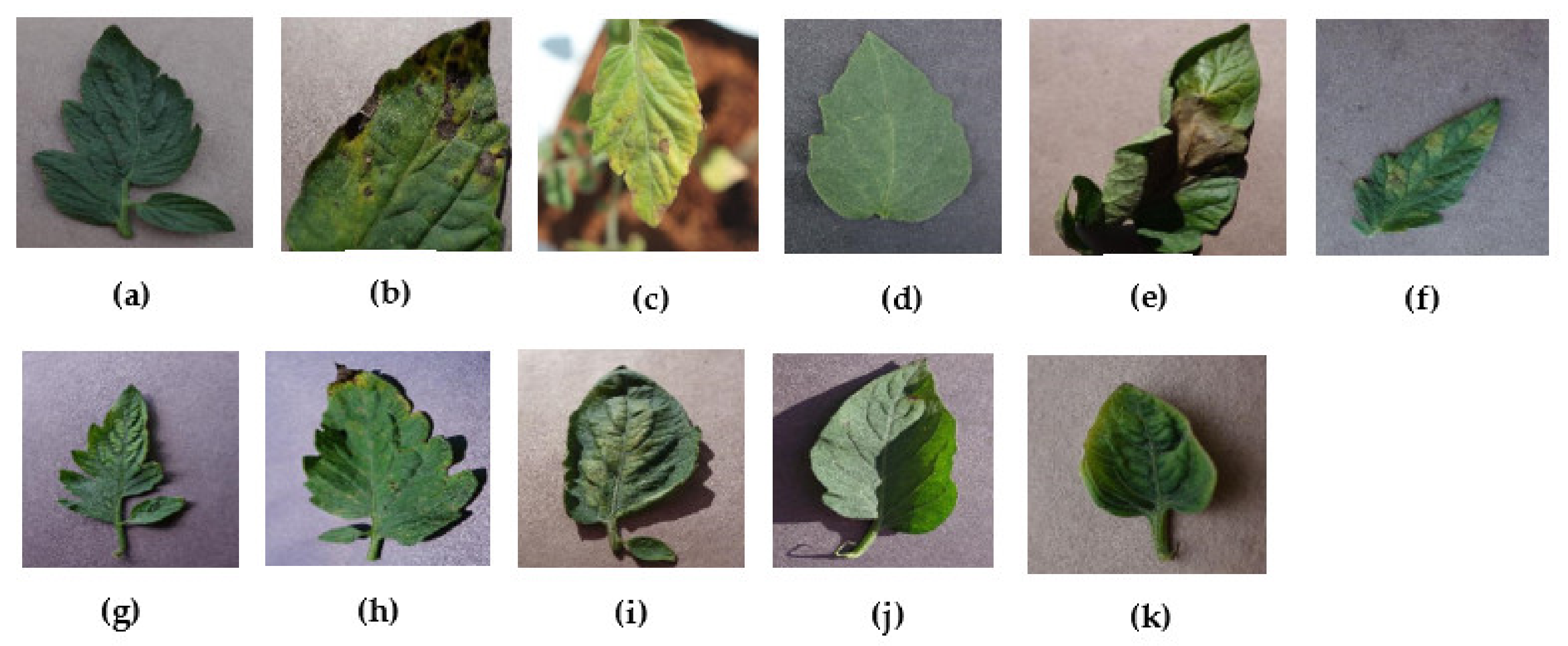
2.1. Data Collection and Preprocessing

Ten classes of tomato leaf images (9 disease and one healthy) that were part of the PlantVillage public datasets [27] were collected. The Fusarium wilt diseased images were captured from the greenhouse located at Gyeongsang National University, South Korea. In this way, a total of 19,510 images from 10 distinct disease classes and one healthy class were used to train, validate, and test the models. Most of the field-captured images were taken nondestructively, but few leaves were detached from the plant and captured on a white background. A sample of images from each class is presented in Figure 1. Similarly, Table 1 shows various information about the dataset, such as class assignment, the common and scientific name of the tomato diseases [13], the number of images per class, and the source of data collection. As image data preparation is very crucial in the deep learning model, different image preprocessing functions were carried out before applying to the model. The main preprocessing functions were labeling, resizing, rescaling, and augmentation of the raw images. Then, the images were split into training, validation, and testing sets at the ratio of 8:1:1 [12]. The larger the number of input images, the better the learning of the deep model. Thus, the image augmentation technique was performed to the training datasets.

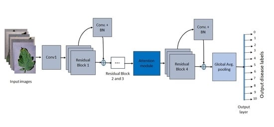
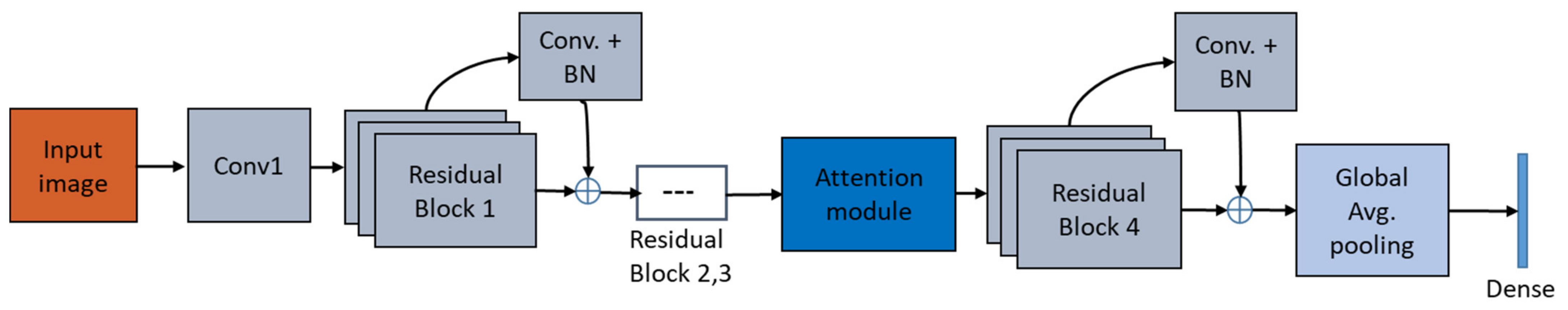
2.2. Lightweight Attention-Based Network Design

A lightweight attention-based CNN model was designed using ResNet topology. It consisted of 20 layers, and the attention modules were embedded between the residual blocks 3 and 4 (after the 16th layer) [16]. Figure 2 shows the block diagram of the proposed model, and the detailed parameters of the base model are given in Table 2. The kernel filters of each layer of the base network were four times lower than the standard ResNet architecture, lowering the total network parameters to make it lighter and portable. In addition, the number of convolutional layers was limited to 20 to decrease the network complexity [28]. Conv1 layer had 16 kernel filters of large patch size (7 × 7) followed by a batch normalization layer, a rectifier linear unit (ReLU) activation layer, and a maximum pooling layer (Max. pooling), which reduced the size of feature maps to half of the input image size. Residual blocks 1 and 4 comprise a convolutional block containing three convolutional layers (conv.) accompanied by a batch normalization (BN) layer and an activation (ReLU) layer. Whereas Residual blocks 2 and 3 have a convolutional block followed by an identity block. The structure of the identity block was similar to the convolutional block except for the shortcut path. Finally, a global average pooling (Global Avg. Pooling) layer converted 2D feature maps to 1D before a dense output layer. The various attention modules were inserted into the base network at the same location, as shown in Figure 2. The necessary zero padding and maximum pooling layers were added to adjust the spatial dimension of the input and output feature maps.

2.2.1. Convolutional Block Attention Module (CBAM)

CBAM uses two attention modules (channel attention and spatial attention) in series, followed by the spatial attention module [15], as shown in Figure 3. The channel attention module was used to generate two feature maps using average and maximum pooling layers from the intermediate layer. Then, both feature maps were input to the shared multilayer perceptron (MLP), and the output feature maps were added before normalizing using the sigmoid function. The multiplied features between the channel attention module and convolutional layer were applied to the spatial attention module to determine the position of the important features in the image. The final feature maps from the channel and spatial attention modules are given in Equations (1) and (2).
CA x   =   σ M L P A v g P o o l x   +   M L P M a x P o o l x
SA x   =   σ f 7 × 7 F a v g s ; F m a x s
where CA(x) represents the channel attention feature maps, SA(x) is the spatial attention feature maps, σ represents the sigmoid function of the feature maps, f 7 × 7 represents the 7 × 7 convolutional operation, M L P is multilayer perceptron, A v g P o o l x is average pooling of input x, M a x P o o l x is the maximum pooling of input x, F m a x s is the feature maps obtained from maximum pooling operation, and F a v g s is the feature maps from maximum pooling operation.

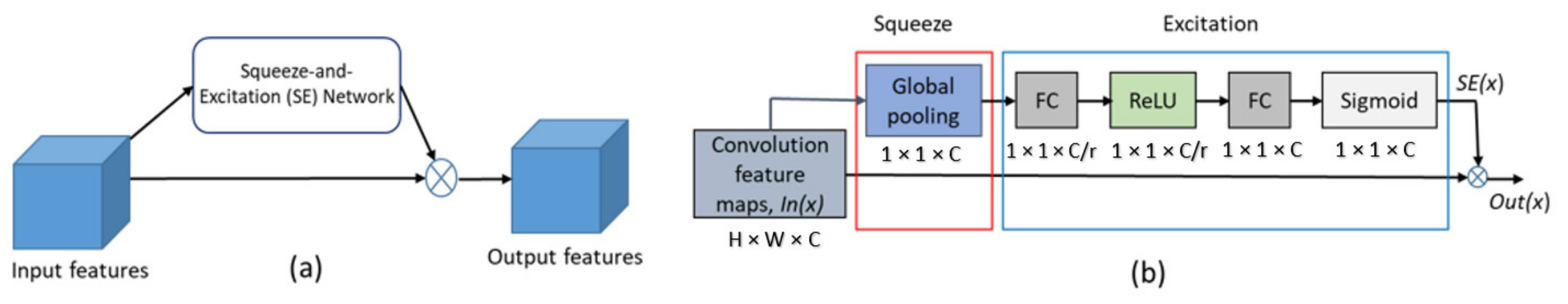
2.2.2. Squeeze-and-Excitation (SE) Attention Module

The dimension of the input feature map was squeezed to 1 × 1 × C by global pooling operation, and two fully connected (FC) layers followed by a rectifier linear unit (ReLU) and sigmoid activation layers were attached to build an excitation block [25], as shown in Figure 4. The squeeze-and-excitation (SE) feature maps were element-wise multiplication, with the input feature maps forwarding to the next layer. The computational operation of the SE module is expressed mathematically in Equation (3). Finally, a mathematical multiplication was carried out to incorporate the SE features maps to the main network’s feature maps.
SE x   =   F e x x , W   =   σ W 2 δ W 1 x
where SE(x) represents the squeeze-and-excitation feature maps, F e x is squeezed or global pooled features, x is the input feature maps, W is the weight of the SE networks, σ is sigmoid operation, δ is ReLU operation, and W 1 and W 2 are the weights of the first and second dense layer, respectively.

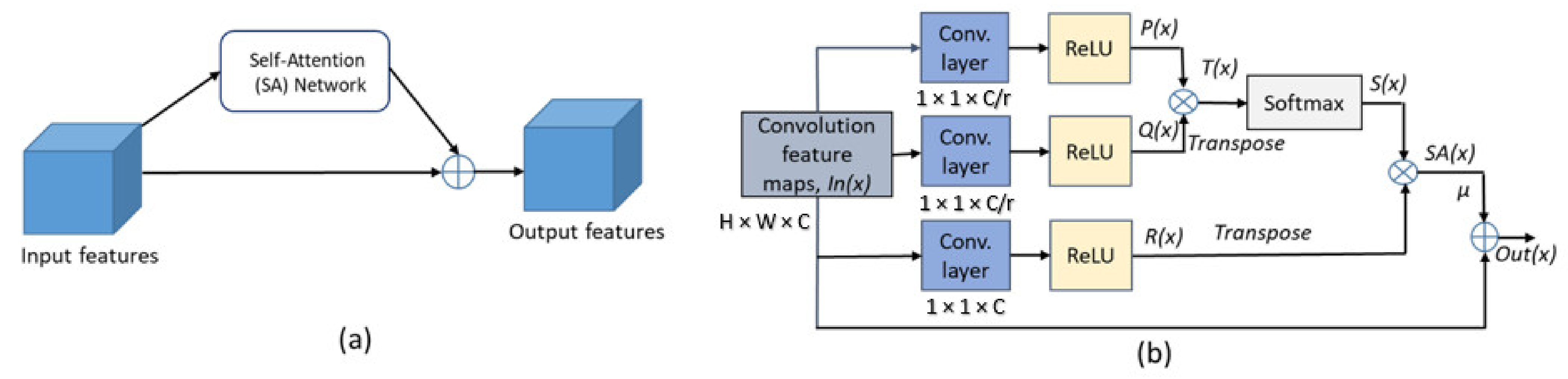
2.2.3. Self-Attention (SA) Module

Figure 5 represents the embedding of a self-attention module into the network and its architecture [16]. It consisted of three parallel convolutional and ReLU activation layers to extract the discriminating features from the input images. The output of the two convolutional layers was multiplied element-wise and fed to a softmax layer to generate an attention map. Then, the attention maps were multiplied by the transpose of the feature maps generated from the third convolutional branch to obtain self-attention feature maps. Finally, scaled attention maps were added to the input feature maps to generate output feature maps, as shown in Equation (4).
O u t x   =   μ SA x   +   I n x   =   μ S x . T x   +   I n x   =   μ S o f t P x . Q x . R x T   +   I n x
where out(x) is output features maps after the self-attention (SA) module, SA(x) is the feature maps after self-attention module, In(x) is the input feature maps, S o f t is softmax operation, μ is a scaling factor, P x , Q x , and R x are the feature maps generated from the three parallel convolutional paths of the SA module, S(x) is the feature maps after softmax operation, and T(x) is the transposed feature maps of the P(x).Q(x).

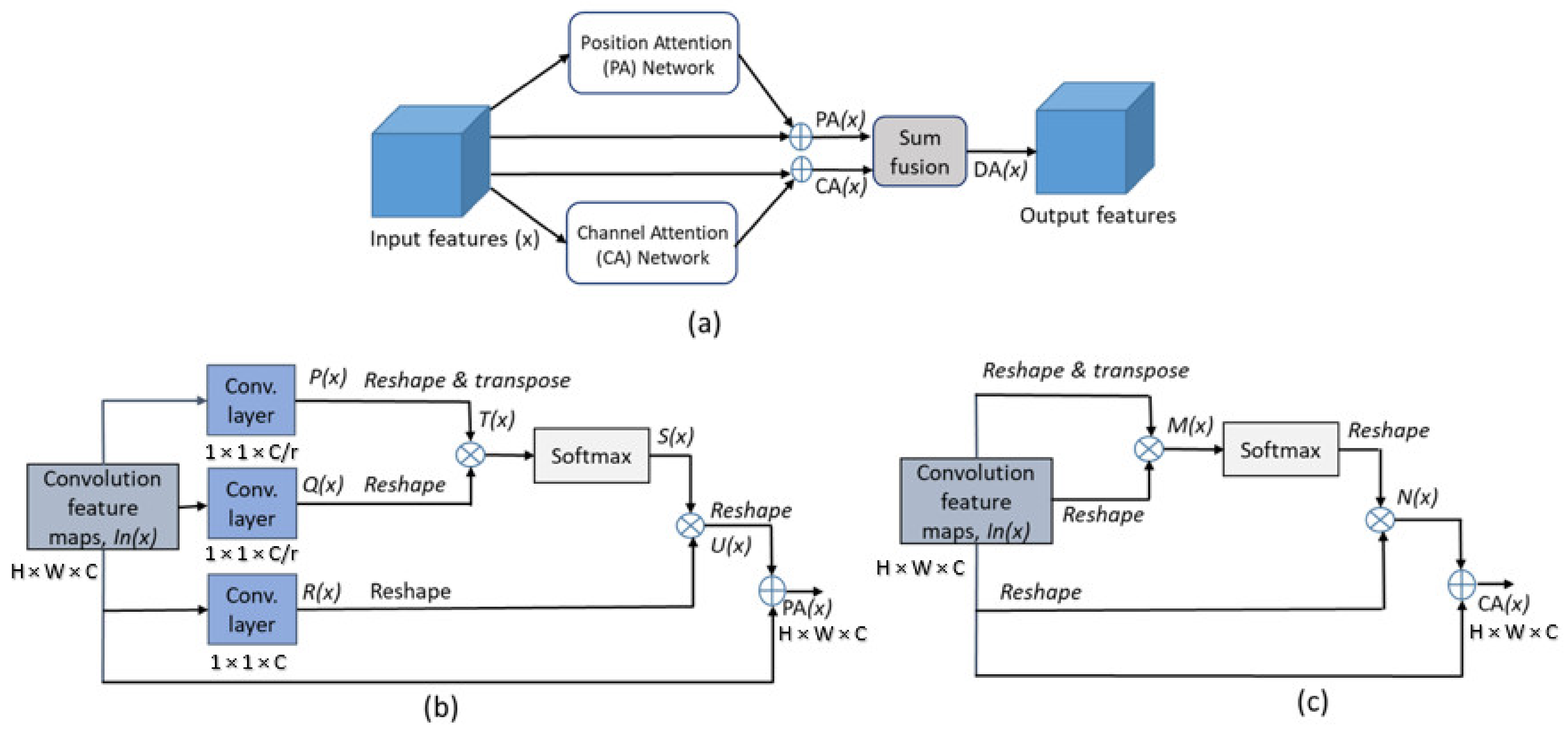
2.2.4. Dual Attention (DA) Module

The authors of [26] proposed a dual attention mechanism with two attention networks, namely position attention (PA) and channel attention (CA) networks for scene segmentation. The position attention network is similar to the self-attention module except for the activation layers and the use of some different strategies for attention map generation, as shown in Figure 6. The DA module also contains a channel attention network that performs two multiplication operations, softmax, and an addition operation. Equation (5) shows the overall mathematical operations carried out in the dual attention module, and Equations (6) and (7) provide the mathematical operation performed in the PA and CA networks.
DA x   =   PA x   +   CA x
PA x   =   U x   +   I n x   =   R x . S x   +   I n x   =   S o f t ( P x T . Q x ) . S x   +   I n x
CA x   =   N x   +   I n x   =   s o f t M x . I n x   +   I n x   =   S o f t ( I n x T . I n x ) . I n x   +   I n x
where DA(x) is the dual attentions’ feature maps, PA(x): position attentions’ feature maps, CA(x): channel attentions’ feature maps, In(x): input feature maps, P(x), Q(x), and R(x): feature maps of three parallel convolutional operations, T(x): transposed P(x).Q(x), S(x): feature maps after the softmax operation of T(x), U(x): multiplied feature maps of S(x) and R(x), CA(x): channel attention feature maps, N(x): multiplied feature of softmax(M(x)) and input feature maps, M(x): multiplied feature maps of reshaped and transposed and reshaped input feature maps, and . and + are the element-wise product and multiplication of the feature maps.

2.3. Network Training and Evaluation

The lightweight base network and all the models with the various attention modules were trained, validated, and tested using the same image datasets. Moreover, the same training hyperparameters and evaluation strategies were applied to fairly compare their performance. As the deep CNN performance improves for a large number of training datasets, we used several data augmentation algorithms, as shown in Table 3. The data augmentation approaches were executed only on training datasets after splitting the whole images into training, validation, and testing sets. The increase in training image count due to the data augmentation process is provided in Table 4. Thus, the training images increased massively after the augmentation (8 times). Furthermore, the Adam optimizer with default learning rate was chosen as training hyperparameter to effectively converge the network [29]. Although the models were trained for a fixed 100 epochs, the optimally trained model was saved for testing purpose in every epoch to ensure minimum validation loss. Furthermore, an Adam optimizer that effectively converges the network [29] was chosen. Then, all the trained models were evaluated using the same testing datasets. The performance of the models was quantified by adopting the standard classification metrics, as shown in Equations (8)–(11) [30]. In addition, the size of the models was determined by counting the total number of network parameters and the memory space usage. On the other hand, the computational complexity was determined using the floating point operations (FLOPs), the total mathematical operations required to complete a forward and backpropagation of an input image.
P r e c i s i o n   =   T P T P + F P
R e c a l l = T P T P + F N
F 1 s c o r e = 2 × P r e c i s i o n × R e c a l l P r e c i s i o n + R e c a l l
A c c u r a c y = T P + T N T P + T N + F P + F N
where T P stands for true positive, T N for true negative, F P is false positive, and F N is false negative of the predicted class.
The training, validation, and testing of all the models were done in the same hardware and software environment. A workstation with Intel Core 10th generation i9-10900K processor, an NVIDIA RTX 2070 GPU (8 GB dedicated memory), and 64 GB DDR4 RAM with Windows 10 Pro, Redmond, WA, USA, operating system was used. Keras with TensorFlow 2.4.1, Santa Clara, CA, USA, running at the backend, CUDA Toolkit 11.0, Santa Clara, CA, USA, cuDNN v8.2.0, Santa Clara, CA, USA, and Python 3.8.3, Wilmington, DE, USA, were used in this study.

3. Results

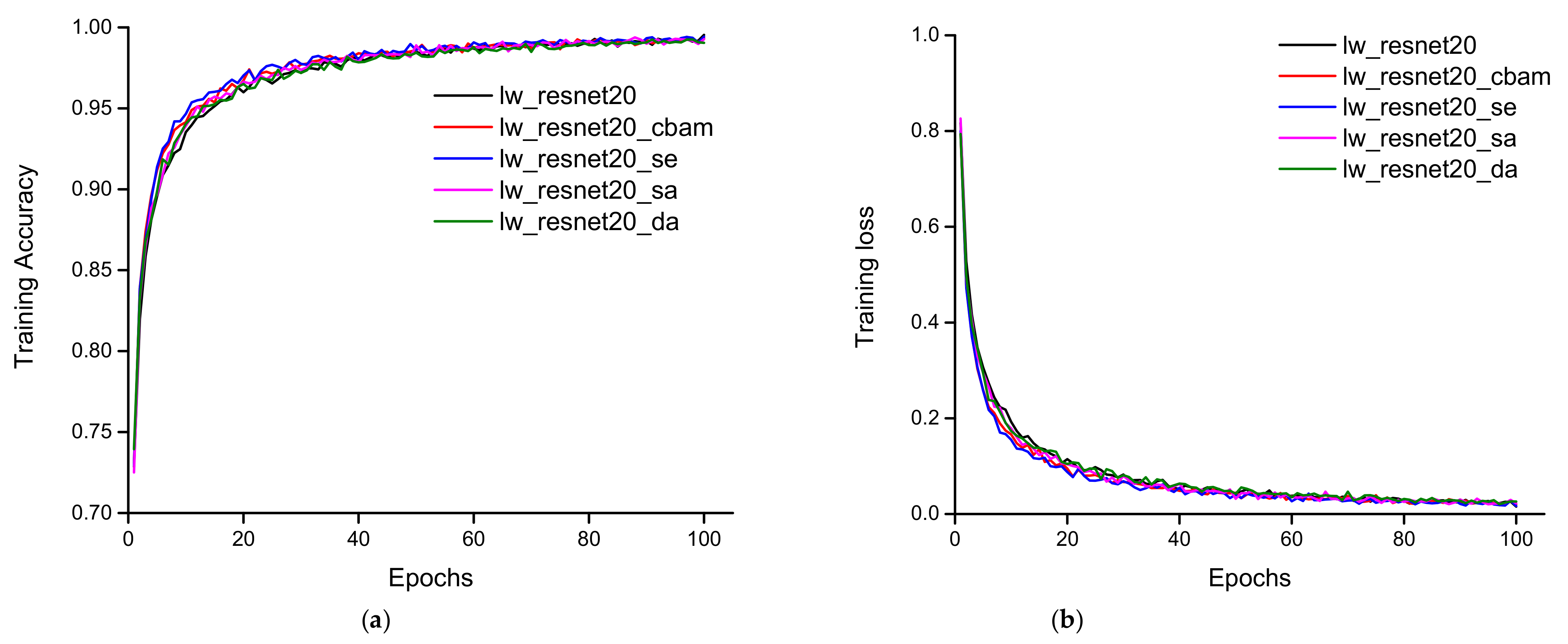
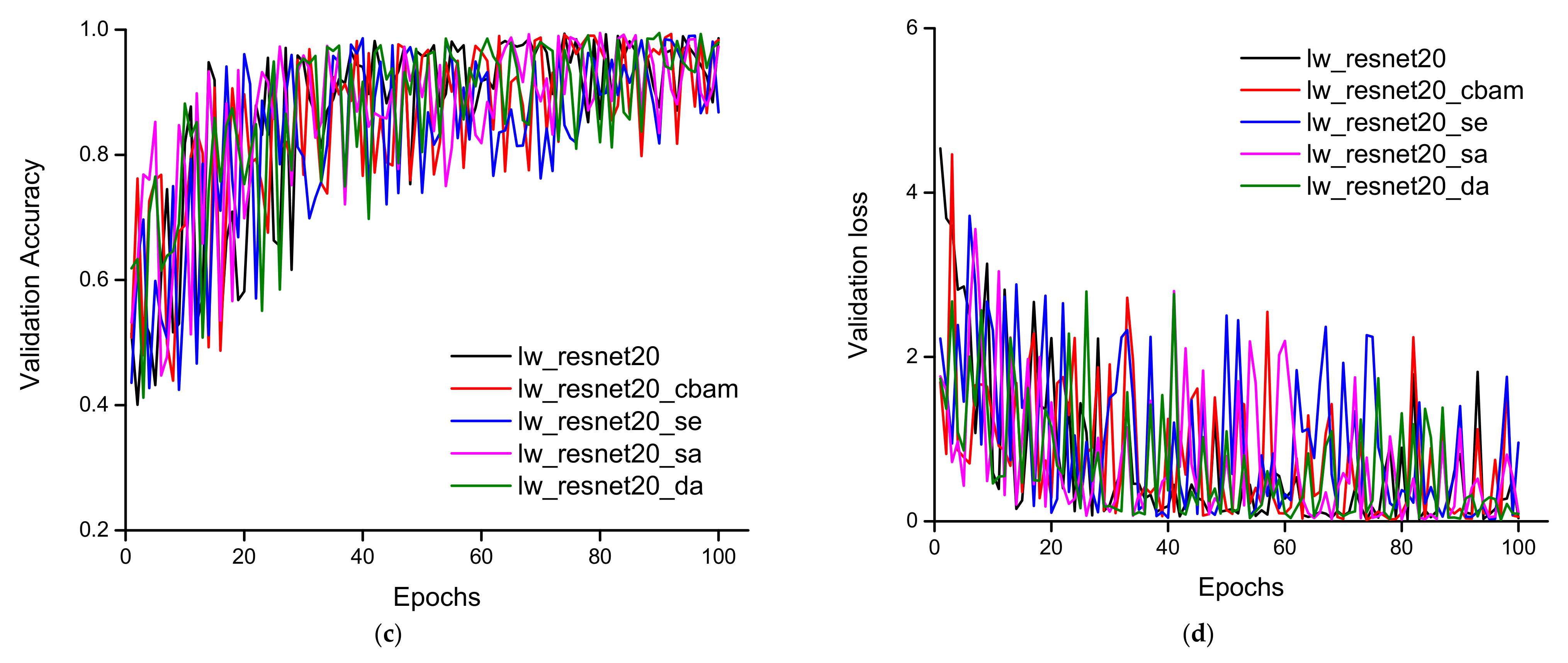
3.1. Training, Validation, and Testing Accuracy of the Models

All the models were trained and validated with the same dataset, training, and validation parameters. Figure 7 shows the training and validation accuracy and loss plots of the different models. The base model without attention module (lw_resnet20) trained relatively slower (indicated by a black line) than the model with attention modules. The model with SE attention module (lw_resnet20_se, represented by a blue line) showed quick training ability, as shown in Figure 7a,b. The validation accuracy and loss of all the models provided a significant fluctuation in each epoch. The best training accuracy and loss were obtained from the base model, followed by the lw_resnet20_se model. However, the highest validation accuracy and loss results were achieve by the lw_resnet20_cbam model, followed by the lw_resnet20_da model, as shown in Table 5.
The optimally trained model was saved using the validation loss checkpoint and recalled to evaluate the testing dataset. The testing dataset, which was not applied to the model training and validation process, was used to check the robustness of the model. A total of 1960 images from 11 distinct classes of tomato leaf (10 disease classes and one healthy class) were utilized while testing the models. The confusion matrix, a summarized and graphical way of visualizing classification performance, was adopted to observe the class-wise classification results of the models. Figure 8 demonstrates the normalized confusion matrices generated from the base model and without various attention mechanisms. The diagonal value represents the ratio of correctly detected images of a particular class to the total number of applied images in that class. The lw_resnet20_cbam model showed an excellent classification capability for all classes of tomato disease. The lw_resnet20_sa model was the second best, correctly classifying more than 97% of all disease classes. On the other hand, the lw_resnet20_se showed the least detection accuracy for target spot diseased images (Figure 8c). The class-wise precision, recall, and F1 score produced by the various models on the test images are presented in Table 6. The lw_resnet20_cbam model performed the best with more than 99% precision, recall, and F1 score in each class classification, providing an average accuracy of 99.69%, followed by the lw_resnet20_sa model. The results in Table 4 show that the attention module helped improve the performance of conventional CNN as the base model produced the lowest average accuracy. However, the different attention strategies influenced the classification ability differently.

3.2. Network Parameters and Efficiency

The deeper the network, the more network parameters there are, thus increasing the size and computational complexity of the network [31]. The network parameters, size, training and testing efficiency, FLOPs, and the average accuracy on the test dataset are presented in Table 7. The proposed models had almost 16 times fewer network parameters and were 23 times less complex than the standard ResNet50 model [15]. The base model was found to be comparatively efficient and lightweight due to fewer network parameters but showed poor performance on the test dataset. The SE and CBAM modules are the lightest attention modules compared to SA and DA. Moreover, the channel attention of CBAM and the module structure of SE are somewhat similar except for the maximum pooling layers. The training time of the models was not significantly different amongst the various attention modules. The test time per image of the model was calculated by averaging the time taken to detect 1960 test images. The SA and DA modules are heavier than CBAM and SE, increasing the computational complexity.

4. Discussion

4.1. Tomato Disease Detection

The low interclass variance, high intra-class variance, and mixed symptoms of two or more diseases on the same leaf are some of the serious challenges for plant disease detection using computer vision techniques [9]. As all the images were of tomato leaves, the chances of producing false positive (FP) and false negative (FN) were higher due to lower interclass variance. Moreover, some of the images of late blight and target spot disease were in the preliminary stage, so there was marginal difference between diseased images and healthy images or mistakenly labeled ones, as shown in Figure 9. Therefore, most of the models poorly detected early blight, healthy, late blight, and target spot leaf images. In contrast, all the models perfectly identified the Fusarium wilt diseased images because of the distinction in datasets. The majority of the Fusarium wilt images were captured directly on the plant (nondestructively), which made them unique with the background and leaf position (Figure 1). The precision, recall, and F1 score of the target spot class were minimum for all the models due to higher FPs and FNs. All models wrongly detected some healthy images as late blight, bacterial spot, and target spot diseases except the lw_resnet20_cbam model, which falsely identified 1% of target spot images as healthy leaves because some diseased images at a very early stage were almost visually indistinguishable from healthy leaves. Therefore, all the models failed to achieve 100% correct classification of healthy and diseased images. However, lw_resnet20_cbam and lw_resnet20_sa models performed well except for giving 1% FPs and FNs, respectively. On the other hand, almost all the models precisely identified bacterial spot, leaf mold, mosaic virus, and yellow leaf curl virus diseased images.

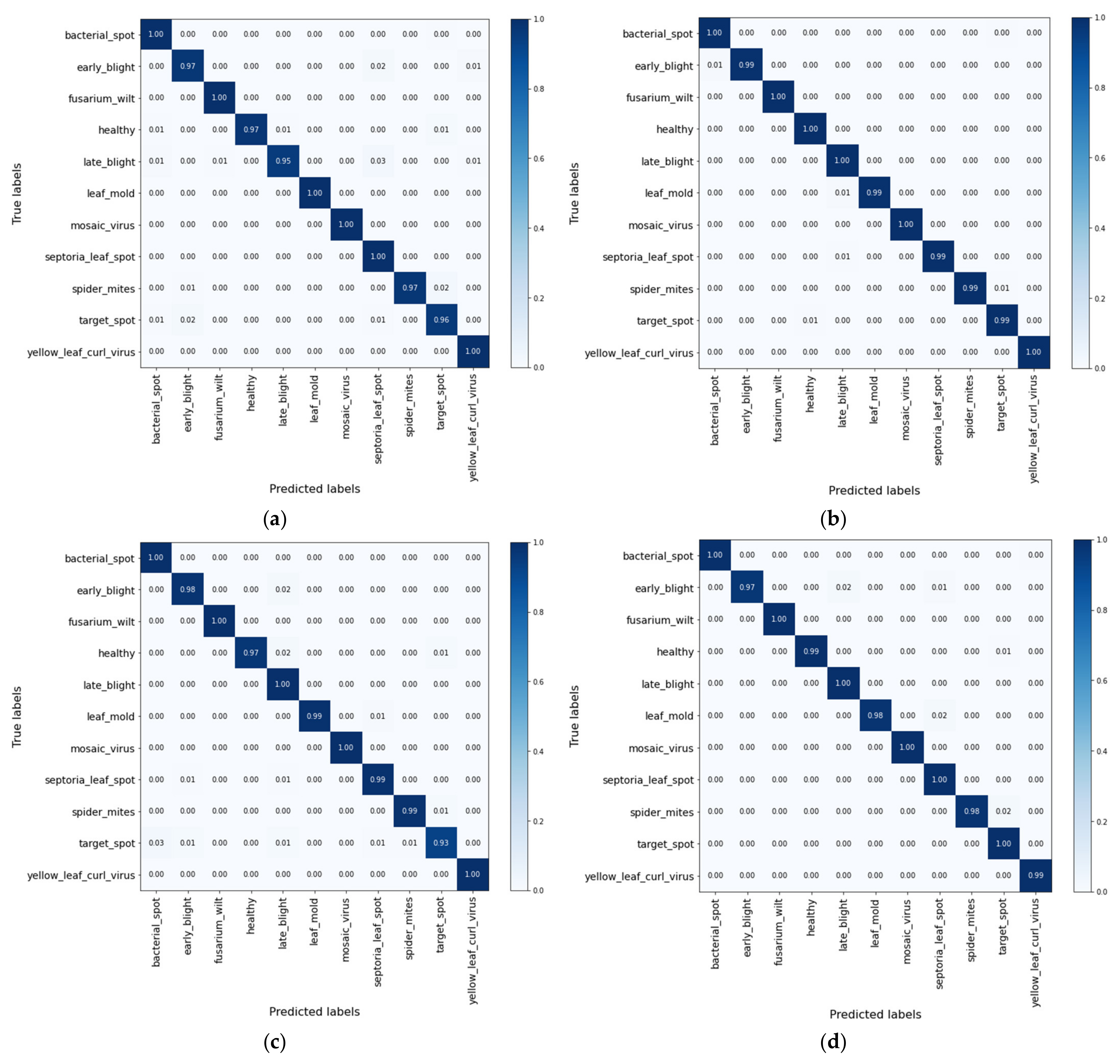
4.2. Performance Evaluation of the Models

The attention modules allow the network to identify the discriminative features and their location in the input images to emphasize key features during training. The channel attention module determines the salient features available in the input images. At the same time, the spatial or position attention reveal the spatial location of those key features. The number of attention modules and their place in the network is same for all. We fixed the position of the attention module between blocks 3 and 4 to permit the network to focus on specific high-level features because the datasets were of the same plant (tomato). The lw_resnet20_cbam outperformed in terms of classification accuracy and model lightness. The additional maximum pooling layer in the channel attention module of the CBAM provide even minute details of the salient features to the network, boosting the network’s performance. DA also uses two attention modules (channel and position), but it failed to perform as well as the CBAM model. One reason for the lower performance might be the parallel combination of channel and position attention. As [15] suggests, series combination results are better than parallel. Moreover, the module structure is bulkier than other attention modules due to three parallel convolutional layers for position attention and three branching matrix operations of input feature maps for channel attention. In contrast, CBAM uses maximum, average pooling, and convolutional layers in the spatial attention module, which is computationally more efficient than matrix operations.
The performance of our proposed model (lw_resnet20_cbam) was compared with models that were previously studied by various researchers. Some studies utilized the same tomato disease datasets with different deep CNN architectures. Some of them also implemented attention-based CNN to improve detection accuracy. Table 8 demonstrates the performance comparison of various CNN architectures used for the same tomato disease datasets. Only [2] used more tomato disease datasets (12 classes) than ours (11 categories). In addition, most researchers applied a generic model designed for a large number of image classification datasets, which is computationally inefficient for a small number of plant datasets. Moreover, the majority of generic models were used as transfer learning. From the table, it can be seen that none of the previous studies achieved better detection results than ours in such a large number of tomato leaf images with such a lightweight model. Therefore, this study will be helpful for future researchers to design efficient and effective networks for portable devices.
Amongst the various attention modules, the SA module also showed competitive results although it came at the cost of more network complexity and size. Its architecture is almost similar to the position attention module of the DA network except for an additional ReLU activation layer in each convolutional branch. In addition, the SA model’s performance superseded the DA model but could not match up to the CBAM model. The SE network utilizes a similar principle as CBAM’s channel attention module, although it only uses global average pooling operation in contrast to the maximum and global pooling operations in CBAM. Nevertheless, its performance was similar to the DA model. However, the SE module is the lightest and most efficient attention module. Thus, it is equally important to identify key features and their locations in the input images. Furthermore, the channel and spatial attention module should be in series so that the model can detect dominant features and their place in the input images.

5. Conclusions

This study experimented with various attention modules and analyzed their performance in tomato disease classification. Attention modules used for different purposes were employed. The network architecture, computational complexity, and performance were comprehensively compared. From the results, it can be concluded that the determination of key features and their location in the input images is crucial to enhancing classification performance. Moreover, identifying key feature regions is wiser than finding essential features. The determination of critical features and their position should be sequential because merging these features will lead to loss of crucial information. Our proposed model outperformed the prevailing generic models used for plant disease detection in terms of accuracy and efficiency.

Author Contributions

Conceptualization, methodology, software, validation, formal analysis, investigation, and writing, A.B.; visualization, E.A. and J.K.B.; supervision, H.-T.K.; project administration, N.-E.K. All authors have read and agreed to the published version of the manuscript.

Funding

This work was supported by the Korea Institute of Planning and Evaluation for Technology in Food, Agriculture, Forestry, and Fisheries (IPET) through Agriculture, Food, and Rural Affairs Convergence Technologies Program for Educating Creative Global Leader, funded by the Ministry of Agriculture, Food, and Rural Affairs (MAFRA) (717001-7).

Data Availability Statement

The data presented in this study are openly available in [PlantVillage] at [www.plantvillage.org], reference number [27].

Conflicts of Interest

The authors declare no conflict of interest.

References

  1. Food and Agriculture Organization of the United Nations [FAO]. Fao Publications Catalogue 2019; FAO: Rome, Italy, 2019; p. 114. [Google Scholar]
  2. Liu, J.; Wang, X. Tomato Diseases and Pests Detection Based on Improved Yolo V3 Convolutional Neural Network. Front. Plant Sci. 2020, 11, 1–12. [Google Scholar] [CrossRef] [PubMed]
  3. Wang, G.; Sun, Y.; Wang, J. Automatic Image-Based Plant Disease Severity Estimation Using Deep Learning. Comput. Intell. Neurosci. 2017, 2017, 2917536. [Google Scholar] [CrossRef] [PubMed] [Green Version]
  4. FAO. Climate-Related Transboundary Pests and Diseases; FAO: Rome, Italy, 2008; p. 59. [Google Scholar]
  5. Fukushima, K. Neocognitron: A self-organizing neural network model for a mechanism of pattern recognition unaffected by shift in position. Biol. Cybern. 1980, 36, 193–202. [Google Scholar] [CrossRef] [PubMed]
  6. LeCun, Y.; Boser, B.; Denker, J.S.; Henderson, D.; Howard, R.E.; Hubbard, W.; Jackel, L.D. Backpropagation applied to digit recognition. Neural Comput. 1989, 1, 541–551. [Google Scholar] [CrossRef]
  7. Krizhevsky, A.; Sutskever, I.; Hinton, G.E. ImageNet classification with deep convolutional neural networks. Commun. ACM 2017, 60, 84–90. [Google Scholar] [CrossRef]
  8. Gomes, J.F.S.; Leta, F.R. Applications of computer vision techniques in the agriculture and food industry: A review. Eur. Food Res. Technol. 2012, 235, 989–1000. [Google Scholar] [CrossRef]
  9. Garcia, J.; Barbedo, A. A review on the main challenges in automatic plant disease identification based on visible range images. Biosyst. Eng. 2016, 144, 52–60. [Google Scholar] [CrossRef]
  10. Bhujel, A.; Khan, F.; Basak, J.K.; Jaihuni, M.; Sihalath, T.; Moon, B.E.; Park, J.; Kim, H.T. Detection of gray mold disease and its severity on strawberry using deep learning networks. J. Plant Dis. Prot. 2022. (Accepted). [Google Scholar]
  11. Toda, Y.; Okura, F. How Convolutional Neural Networks Diagnose Plant Disease. Plant Phenomics 2019, 2019, 9237136. [Google Scholar] [CrossRef]
  12. Mohanty, S.P.; Hughes, D.P.; Salathé, M. Using deep learning for image-based plant disease detection. Front. Plant Sci. 2016, 7, 1–10. [Google Scholar] [CrossRef] [Green Version]
  13. Ferentinos, K.P. Deep learning models for plant disease detection and diagnosis. Comput. Electron. Agric. 2018, 145, 311–318. [Google Scholar] [CrossRef]
  14. Mnih, V.; Heess, N.; Graves, A.; Kavukcuoglu, K. Recurrent models of visual attention. In Proceedings of the Advances in Neural Information Processing Systems: Annual Conference on Neural Information Processing Systems 2014, Montreal, QC, Canada, 8–13 December 2014; Volume 3, pp. 2204–2212. [Google Scholar]
  15. Woo, S.; Park, J.; Lee, J.Y.; Kweon, I.S. CBAM: Convolutional block attention module. In Proceedings of the Computer Vision—ECCV 2018, Munich, Germany, 8–14 September 2018; Volume 11211, pp. 3–19. [Google Scholar] [CrossRef] [Green Version]
  16. Zeng, W.; Li, M. Crop leaf disease recognition based on Self-Attention convolutional neural network. Comput. Electron. Agric. 2020, 172, 105341. [Google Scholar] [CrossRef]
  17. Lee, S.H.; Goëau, H.; Bonnet, P.; Joly, A. Attention-Based Recurrent Neural Network for Plant Disease Classification. Front. Plant Sci. 2020, 11, 1–8. [Google Scholar] [CrossRef]
  18. Zhao, S.; Peng, Y.; Liu, J.; Wu, S. Tomato leaf disease diagnosis based on improved convolution neural network by attention module. Agriculture 2021, 11, 651. [Google Scholar] [CrossRef]
  19. Yilma, G.; Belay, S.; Kumie, G.; Assefa, M.; Ayalew, M.; Oluwasanmi, A.; Qin, Z. Attention augmented residual network for tomato disease detection and classification. Turkish J. Electr. Eng. Comput. Sci. 2021, 29, 2869–2885. [Google Scholar] [CrossRef]
  20. Yang, G.; He, Y.; Yang, Y.; Xu, B. Fine-Grained Image Classification for Crop Disease Based on Attention Mechanism. Front. Plant Sci. 2020, 11, 1–15. [Google Scholar] [CrossRef]
  21. Brahimi, M.; Boukhalfa, K.; Moussaoui, A. Deep Learning for Tomato Diseases: Classification and Symptoms Visualization. Appl. Artif. Intell. 2017, 31, 299–315. [Google Scholar] [CrossRef]
  22. Rangarajan, A.K.; Purushothaman, R.; Ramesh, A. Tomato crop disease classification using pre-trained deep learning algorithm. Procedia Comput. Sci. 2018, 133, 1040–1047. [Google Scholar] [CrossRef]
  23. Tm, P.; Pranathi, A.; Saiashritha, K.; Chittaragi, N.B.; Koolagudi, S.G. Tomato Leaf Disease Detection Using Convolutional Neural Networks. In Proceedings of the 2018 11th International Conference on Contemporary Computing (IC3), Noida, India, 2–4 August 2018. [Google Scholar] [CrossRef]
  24. He, K.; Zhang, X.; Ren, S.; Sun, J. Deep residual learning for image recognition. In Proceedings of the IEEE Conference on Computer Vision and Pattern Recognition (CVPR), Las Vegas, NV, USA, 27–30 June 2016. [Google Scholar] [CrossRef] [Green Version]
  25. Hu, J.; Shen, L.; Albanie, S.; Sun, G.; Wu, E. Squeeze-and-Excitation Networks. IEEE Trans. Pattern Anal. Mach. Intell. 2020, 42, 2011–2023. [Google Scholar] [CrossRef] [Green Version]
  26. Fu, J.; Liu, J.; Tian, H.; Li, Y.; Bao, Y.; Fang, Z.; Lu, H. Dual attention network for scene segmentation. In Proceedings of the IEEE/CVF Conference on Computer Vision and Pattern Recognition (CVPR), Long Beach, CA, USA, 15–20 June 2019. [Google Scholar] [CrossRef] [Green Version]
  27. Hughes, D.P.; Salathe, M. An open access repository of images on plant health to enable the development of mobile disease diagnostics. arXiv 2015, arXiv:1511.08060. [Google Scholar]
  28. Koning, S.; Greeven, C.; Postma, E. Reducing Artificial Neural Network Complexity: A Case Study on Exoplanet Detection Related Work on Parameter Reduction. arXiv 2015, arXiv:1902.10385. [Google Scholar]
  29. Kingma, D.P.; Ba, J.L. Adam: A method for stochastic optimization. In Proceedings of the International Conference on Learning Representations (ICLR), San Diego, CA, USA, 7–9 May 2015; pp. 1–15. [Google Scholar]
  30. Grandini, M.; Bagli, E.; Visani, G. Metrics for Multi-Class Classification: An Overview. arXiv 2020, arXiv:2008.05756. [Google Scholar]
  31. Vu, T.; Wen, E.; Nehoran, R. How Not to Give a FLOP: Combining Regularization and Pruning for Efficient Inference. arXiv 2020, arXiv:2003.13593. [Google Scholar]
  32. Abbas, A.; Jain, S.; Gour, M.; Vankudothu, S. Tomato plant disease detection using transfer learning with C-GAN synthetic images. Comput. Electron. Agric. 2021, 187, 106279. [Google Scholar] [CrossRef]
  33. Maeda-Gutiérrez, V.; Galván-Tejada, C.E.; Zanella-Calzada, L.A.; Celaya-Padilla, J.M.; Galván-Tejada, J.I.; Gamboa-Rosales, H.; Luna-García, H.; Magallanes-Quintanar, R.; Guerrero Méndez, C.A.; Olvera-Olvera, C.A. Comparison of Convolutional Neural Network Architectures for Classification of Tomato Plant Diseases. Appl. Sci. 2020, 10, 1245. [Google Scholar] [CrossRef] [Green Version]
  34. Zhang, K.; Wu, Q.; Liu, A.; Meng, X. Can deep learning identify tomato leaf disease? Adv. Multimed. 2018, 2018, 6710865. [Google Scholar] [CrossRef] [Green Version]
  35. Trivedi, N.K.; Gautam, V.; Anand, A.; Aljahdali, H.M.; Villar, S.G.; Anand, D.; Goyal, N.; Kadry, S. Early Detection and Classification of Tomato Leaf Disease Using High-Performance Deep Neural Network. Sensors 2021, 21, 7987. [Google Scholar] [CrossRef]
  36. Gonzalez-huitron, V.; Le, A.; Amabilis-sosa, L.E.; Ramírez-pereda, B.; Rodriguez, H. Disease detection in tomato leaves via CNN with lightweight architectures implemented in Raspberry Pi 4. Comput. Electron. Agric. 2021, 181, 105951. [Google Scholar] [CrossRef]
  37. Ramamurthy, K.; Hariharan, M.; Sundar, A.; Mathikshara, P.; Johnson, A.; Menaka, R. Attention embedded residual CNN for disease detection in tomato leaves. Appl. Soft Comput. J. 2019, 86, 105933. [Google Scholar] [CrossRef]
Figure 1. Sample image of the dataset. (a) Bacterial spot, (b) early blight, (c) Fusarium wilt, (d) healthy, (e) late blight, (f) leaf mold, (g) mosaic virus, (h) Septoria leaf spot, (i) spider mites; (j) target spot, (k) yellow leaf curl virus.
Agriculture 12 00228 g001
Figure 2. Block diagram of the proposed lightweight model. The attention modules were embedded between residual block 3 and 4, allowing the models to focus on high-level features. In addition, a convolutional layer and a batch normalization layer were attached to the shortcut path. Where, Conv1: Convolutional layer 1, Conv: Convolutional layer, BN: Batch Normalization, and Global Avg. Pooling: Global average pooling.
Agriculture 12 00228 g002
Figure 3. Convolutional block attention module (CBAM) architecture and embedding to the main network. (a) Application of the CBAM in the main network, (b) Channel attention (CA) module architecture, and (c) Spatial attention (SA) module architecture. Where H: Height of the feature map, W: Width of the feature map, C: number of channels or feature maps, and MLP: Multilayer Perceptron.
Agriculture 12 00228 g003
Figure 4. Squeeze-and-excitation (SE) architecture and placement into the main network. (a) Placement of the SE module in the main network and (b) squeeze-and-excitation (SE) module architecture. Where H: height of the feature map, W: width of the feature map, C: number of channels, r: channel reduction ratio (8), FC: fully connected layer, and ReLU: Rectifier linear Unit.
Agriculture 12 00228 g004
Figure 5. Self-attention (SA) architecture and its integration into the main network. (a) Integration of the SA module in the main network and (b) self-attention (SA) module architecture. Where Conv. layer: convolutional layer and ReLU: rectifier linear unit, H: height of the feature map, W: width of the feature map, C: number of channels, r: channel reduction ratio, In(x): input feature maps, P(x): feature maps after the first branch convolutional and ReLU operations, Q(x): feature maps after the second branch convolutional and ReLU operations, R(x): feature maps after the third branch convolutional and ReLU operations, T(x): transposed feature maps of P(x).Q(x), S(x): softmax output of transposed feature maps, SA(x): self-attention feature maps, µ: scaling factor, and Out(x): output feature maps after the SA module.
Agriculture 12 00228 g005
Figure 6. Dual attention (DA) architecture and its application into the main network. (a) Application of the DA module in the main network, (b) position attention (PA) network architecture, and (c) channel attention (CA) network architecture. Where Conv. layer: convolutional layer, P(x), Q(x), and R(x) are the feature maps from the three parallel convolutional operations, H: height of the feature map, W: width of the feature map, C: number of channels, T(x): transposed feature maps of P(x).Q(x), S(x): feature map after the softmax operation of T(x), U(x): reshaped feature maps of S(x).R(x), PA(x): position attention feature maps, In(x): input feature maps of the modules, M(x): feature maps after the multiplication of reshaped and transposed and the input feature maps, N(x): feature maps after the element-wise multiplication of the softmax output of M(x) and reshaped input feature maps, and CA(x): channel attention feature maps.
Agriculture 12 00228 g006
Figure 7. Training and validation accuracy and loss of the models. (a) Training accuracy, (b) training loss, (c) validation accuracy, and (d) validation loss.
Agriculture 12 00228 g007aAgriculture 12 00228 g007b
Figure 8. Confusion matrices provided by various models on the test dataset. (a) Lightweight base model (lw_resnet20), (b) lightweight model with CBAM (lw_resnet20_cbam), (c) model with SE attention module (lw_resnet20_se), (d) SA-based model (lw_resnet20_sa), and (e) DA-based model (lw_resnet20_da).
Agriculture 12 00228 g008aAgriculture 12 00228 g008b
Figure 9. Sample images of different classes with visually similarity. (a) Healthy leaf image, (b) late blight diseased image, and (c) target spot diseased image.
Agriculture 12 00228 g009
Table 1. Details of tomato disease datasets, including assignment of class label, common and scientific names of diseases, number of images per class, and the source of data collection.
Class
Label
Disease Common NameScientific NameImages (No.)Source (%)
PublicField
0Bacterial spotXanthomonas campestris pv. vesicatoria2127100
1Early blight Alternaria solani1000100
2Fusarium wiltFusarium oxysporum f.sp. lycopersici1350-100
3Healthy -1591100
4Late blight Phytophthora infestans1909100
5Leaf moldFulvia fulva952100
6Mosaic virusTomato mosaic virus373100
7Septoria leaf spotSeptoria lycopersici1771100
8Spider mitesTetranychus urticae1676100
9Target spotCorynespora cassiicola1404100
10Yellow leaf curl virusBegomovirus (Fam. Geminiviridae)5357100
Total19,510
Table 2. Detailed architectural parameters of the lightweight ResNet20 base network.
BlockSub-BlockLayerKernel Size, Stride and NumberOutput Shape
Input image Input 256 × 256 × 3
Conv1 Convolutional7 × 7, 2, 16128 × 128 × 16
Residual block1Convolutional block1 × 1, 2, 1663 × 63 × 64
3 × 3, 1, 16
1 × 1, 1, 64
Shortcut1 × 1, 2, 64
Residual block2Convolutional block1 × 1, 2, 3232 × 32 × 128
3 × 3, 1, 32
1 × 1, 1, 128
Shortcut1 × 1, 2, 128
Identity block1 × 1, 1, 32
3 × 3, 1, 32
1 × 1, 1, 128
Residual block3Convolutional block1 × 1, 2, 6416 × 16 × 256
3 × 3, 1, 64
1 × 1, 1, 256
Shortcut1 × 1, 2, 256
Identity block1 × 1, 1, 64
3 × 3, 1, 64
1 × 1, 1, 256
Residual block4Convolutional block1 × 1, 2, 2568 × 8 × 1024
3 × 3, 1, 256
1 × 1, 1, 1024
Shortcut1 × 1, 2, 1024
Global average pooling Global average pooling 1024
Dense Output 11
” represents the same content as the above row (convolutional).
Table 3. Training hyperparameters and details of data augmentation.
Particular Description
Batch size32
Optimizer Adam
Learning rate0.001 (default)
Epoch 100
Data augmentation:
   Image zooming0.2
   Vertical shearing0.2
   Horizontal shearing0.2
   Vertical flipTrue
   Horizontal flipTrue
   Vertical shift0.2
   Horizontal shift0.2
   Image rotation45°
Table 4. Statistics of training, validation, and testing datasets with data augmentation.
Class NameTrainingValidation *Testing *
Original CountAfter Augmentation
Bacterial spot170115,309212214
Early blight 8007200100100
Fusarium wilt10809720135135
Healthy 127211,448159160
Late blight 152713,743190192
Leaf mold76168499596
Mosaic virus29826823738
Septoria leaf spot141612,744177178
Spider mites134012,060167169
Target spot112310,107140141
Yellow leaf curl virus428538,565535537
Total count15,603140,42719471960
* Data augmentation was applied only for training datasets; therefore, the validation and testing data records are not changed.
Table 5. Top-1 training and validation loss and accuracy obtained from different models.
ModelTrainingValidation
LossAccuracyLossAccuracy
lw_resnet200.01550.99540.01940.9936
lw_resnet20_cbam0.01860.99420.01550.9951
lw_resnet20_se0.01690.99420.03000.9905
lw_resnet20_sa0.02050.99380.01980.9947
lw_resnet20_da0.02050.99250.01910.9947
Table 6. Precision, recall, F1 score, and average accuracy, obtained from the base model and models with different attention modules.
* Class Labellw_resnet20lw_resnet20_cbamlw_resnet20_selw_resnet20_salw_resnet20_da
prec.rec.F1 Scoreprec.rec.F1 Scoreprec.rec.F1 Scoreprec.rec.F1 Scoreprec.rec.F1 Score
00.981.000.991.001.001.000.981.000.991.001.001.001.001.001.00
10.960.970.971.000.990.990.970.980.981.000.970.980.950.990.97
20.991.000.991.001.001.001.001.001.001.001.001.000.991.000.99
31.000.970.990.991.001.001.000.970.981.000.991.001.000.970.99
40.990.950.970.991.000.990.961.000.980.991.000.990.980.960.97
51.001.001.001.000.990.991.000.990.991.000.980.990.990.980.98
61.001.001.001.001.001.001.001.001.001.001.001.001.001.001.00
70.961.000.981.000.991.000.990.990.990.981.000.990.971.000.99
81.000.970.981.000.991.000.990.990.950.990.980.990.990.990.99
90.950.960.960.990.990.990.970.930.950.971.000.990.990.980.98
101.001.001.001.001.001.001.001.001.001.000.991.001.001.001.00
Avg. acc.0.98580.99690.98850.99320.9890
* 0: bacterial spot, 1: early blight, 2: Fusarium wilt, 3: healthy, 4: late blight, 5: leaf mold, 6: mosaic virus, 7: Septoria leaf spot, 8: spider mites, 9: target spot, 10: yellow leaf curl virus. prec.: precision, rec.: recall, avg. acc.: average accuracy; lw_resnet20: lightweight ResNet20 base model, lw_resnet20_cbam: lightweight convolutional block attention module (CBAM) model, lw_resnet20_se: lightweight squeeze-and-excitation (SE) model, lw_resnet20_sa: lightweight self-attention (SA) model, lw_resnet20_da: lightweight dual attention (DA) model. The bold face average accuracy is the highest accuracy.
Table 7. Network parameters, training and testing efficiency, network size, and FLOPs of different models.
ModelNetwork
Parameters
Training Time (h:m:s)Test Time per Image (ms)Size on Disk (MB)GFLOPsAverage
Accuracy (%)
lw_resnet201,424,0433:42:470.79516.60.43998.58
lw_resnet20_cbam1,440,8133:45:160.91416.80.44099.69
lw_resnet20_se1,440,7153:43:240.92716.80.44098.85
lw_resnet20_sa1,572,0753:44:140.96118.30.55399.32
lw_resnet20_da1,505,9633:46:270.98417.60.58798.90
Standard ResNet5023,610,2513:45:511.59127010.1098.74
Table 8. Performance comparison of the proposed model with previous studies on tomato disease classification.
ReferenceDeep CNN ArchitectureDatasetsAccuracy (%)Summary
[2]Improved YOLOV312 classes of tomato leaf images92.39Applied feature fusion
technique for tiny disease spot detection.
[18]ResNet50 with squeeze-and-excitation (SE)
attention module
10 classes of tomato leaf and 4 classes of grape leaf images96.81 for tomato and 99.24 for grape
datasets
SE attention module was
implemented into a generic ResNet50 model.
[19]Attention augmented
ResNet (AAR)
10 classes of tomato leaf images98.91Synthetically generates tomato leaf images to increase training datasets.
[22]AlexNet and VGG16
(pretrained)
7 classes of tomato leaf images97.49 for AlexNet and 97.29 for VGG16 modelApplied transfer learning strategy to swallow and medium deep models.
[32]DenseNet121 (pretrained)5, 7, and 10 classes of tomato leaf images99.51, 98.65, and 97.11 for 5, 7, and 10 classes, respectivelyUsed transfer learning with original and synthetically
generated images.
[33]AlexNet, GoogleNet,
Inception V3, ResNet18, and ResNet50
10 classes of tomato leaf images98.93, 99.39, 98.65, 99.06, and 99.15,
respectively
Compared the performances of some standard models.
[34]AlexNet, GoogleNet, and ResNet509 classes of tomato leaf images95.83, 95.66, and 96.51, respectivelyUsed only the diseased images of tomato leaves with generic model.
[35]Customized 11 layer CNN10 classes of tomato leaf images98.49Used a swallow network with 3000 images only.
[36]MobileNetV2, NASNetMobile, Xception, MobileNet V3 (pretrained)75, 84, 100, and 98,
respectively
Used lightweight generic models to deploy in Raspberry Pi.
[37]Attention embedded
ResNet
4 classes of tomato leaf images98Applied an attention-based swallow ResNet model for small datasets.
Our modelLightweight CBAM attention module-based
ResNet20
(lw_resnet20_cbam)
11 classes of tomato leaf images99.69Reduced the network
parameters and complexity of backbone network and improved performance using an effective attention module.
CNN: Convolutional Neural Network, YOLO: You Looks Only Once, ResNet: Residual Network, VGG: Visual Geometry Group, MobileNet: Mobile Network, NASNetMobile: Neural Architecture Search Network Mobile, and CBAM: Convolutional Block Attention Module. ” represents the same content as the above row.
Publisher’s Note: MDPI stays neutral with regard to jurisdictional claims in published maps and institutional affiliations.

