
Rice Growth Stage Classification via RF-Based Machine Learning and Image Processing
 ,
,
Abstract
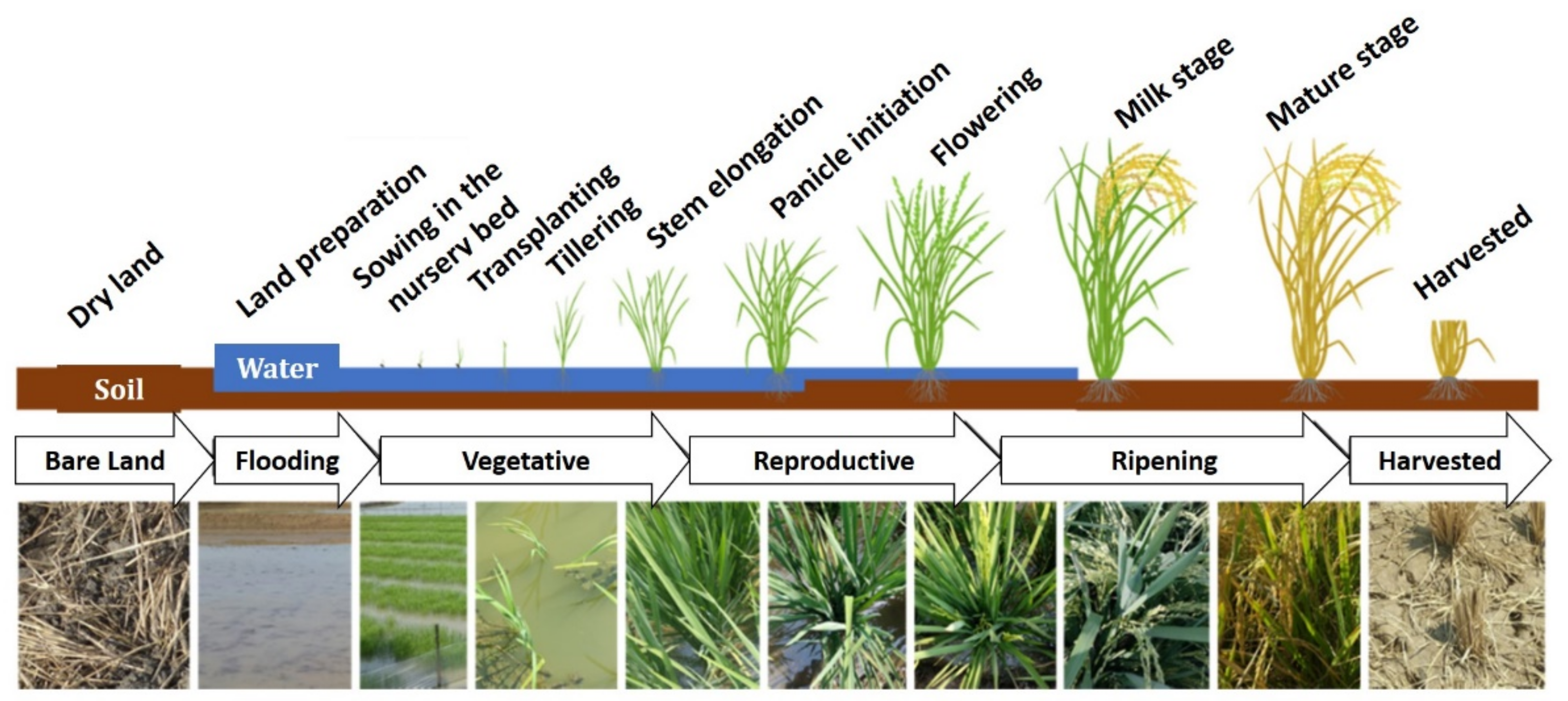
:1. Introduction
2. Background and Related Work
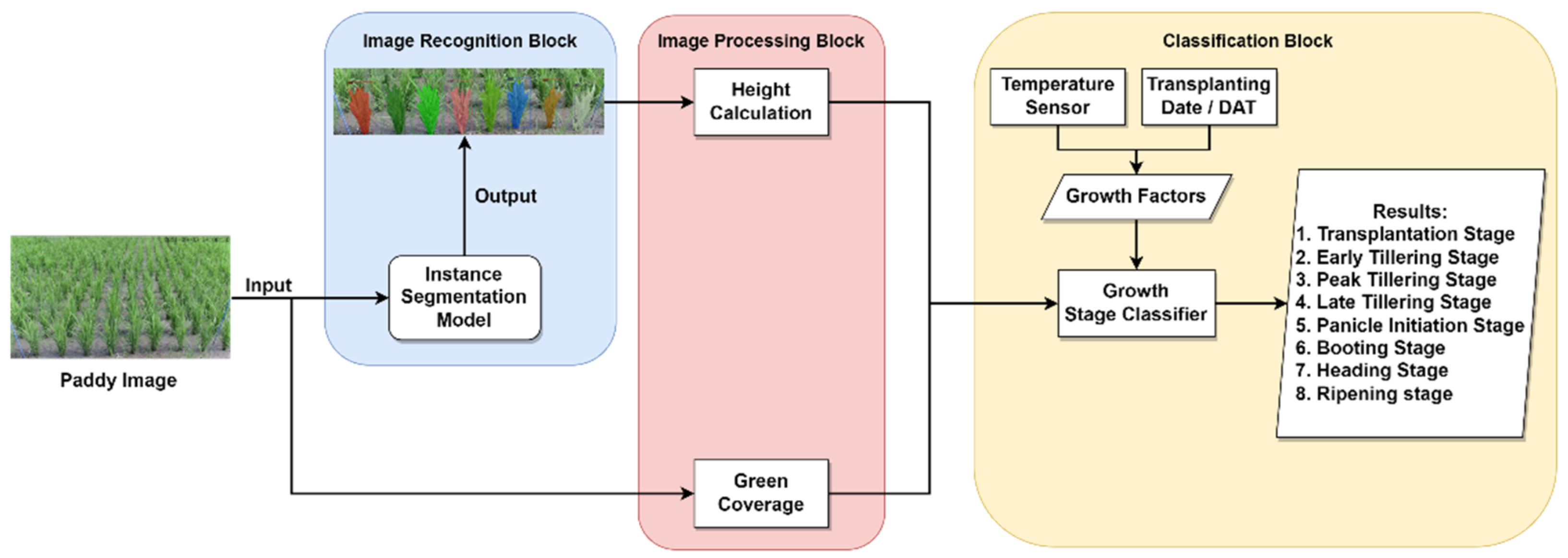
3. Design and Implementation
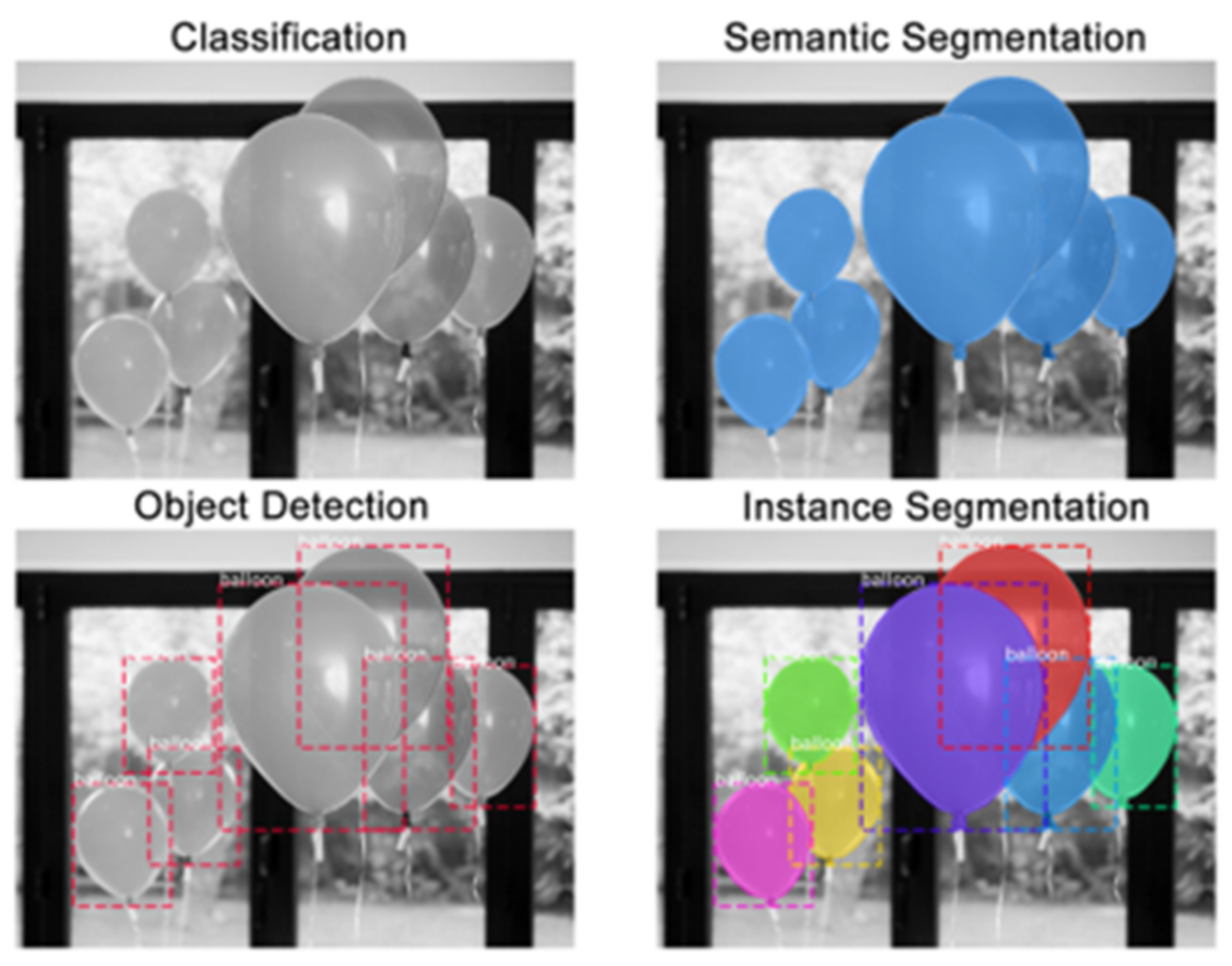
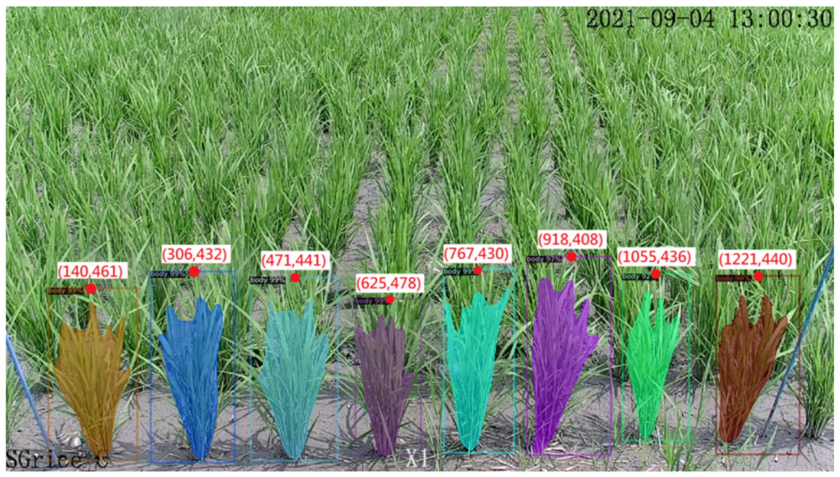
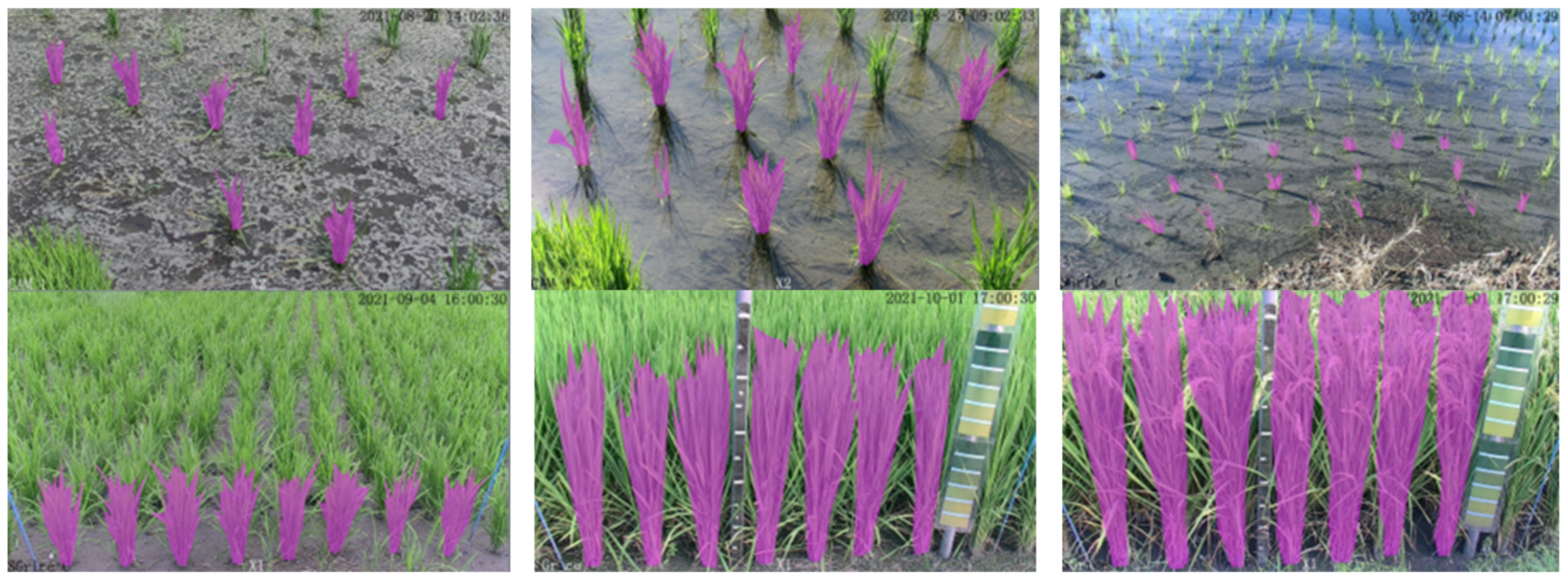
3.1. Image Recognition
3.2. Instance Segmentation Model
3.3. Data Collection and Training Setup
3.4. Image Processing
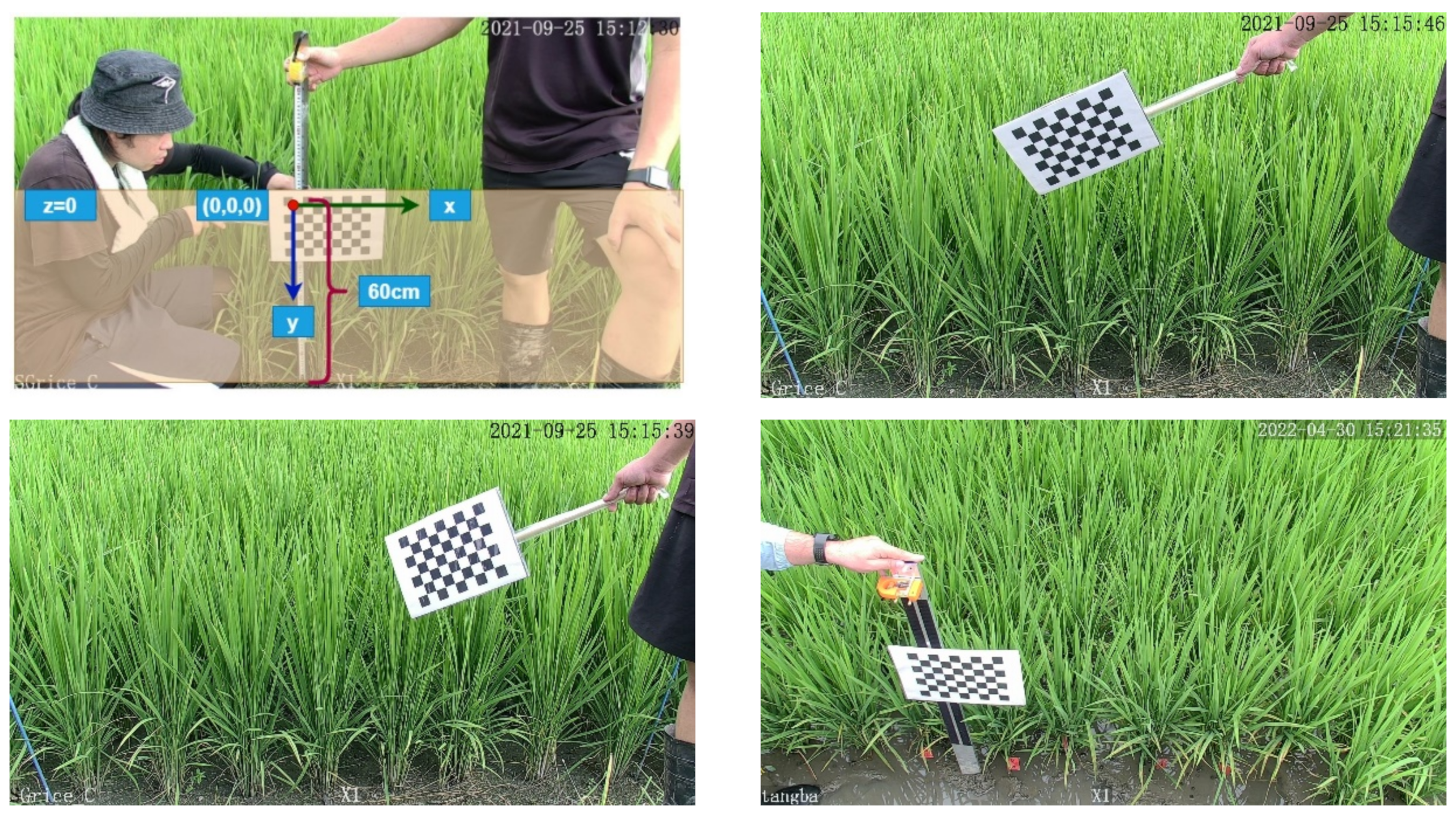
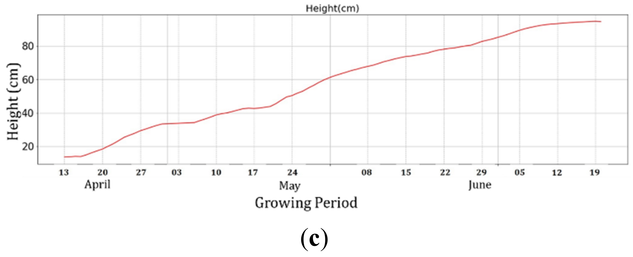
3.4.1. Height Calculation Using Camera Calibration
- Define real-world coordinates of 3D points using a known-size chessboard.
- Capture different viewpoints of the chessboard.
- Find the pixel coordinates (u, v) for each 3D point in different images (use findChessboardCorners() method from OpenCV)
- Find camera parameters (use the calibrateCamera() method from OpenCV).
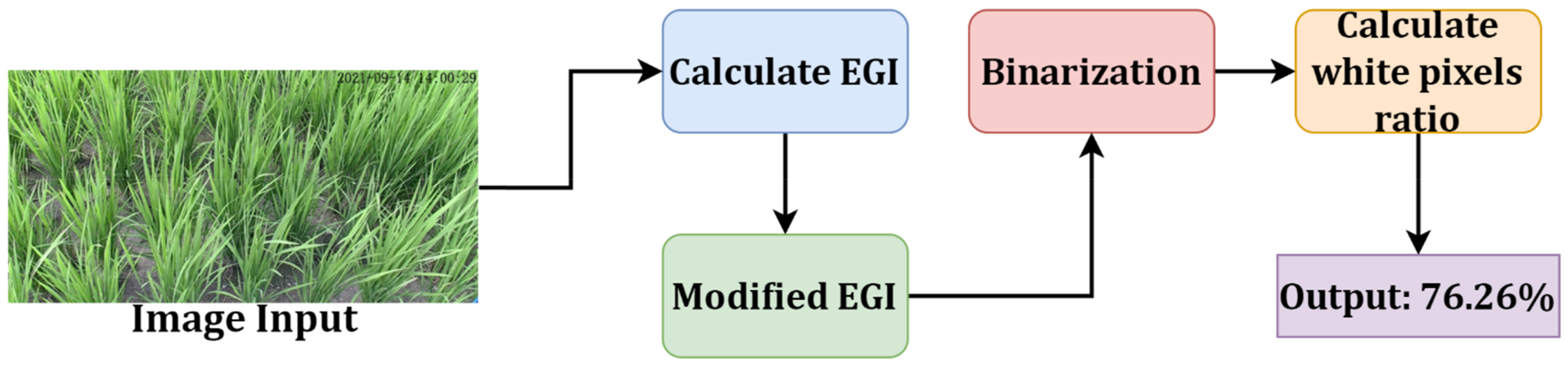
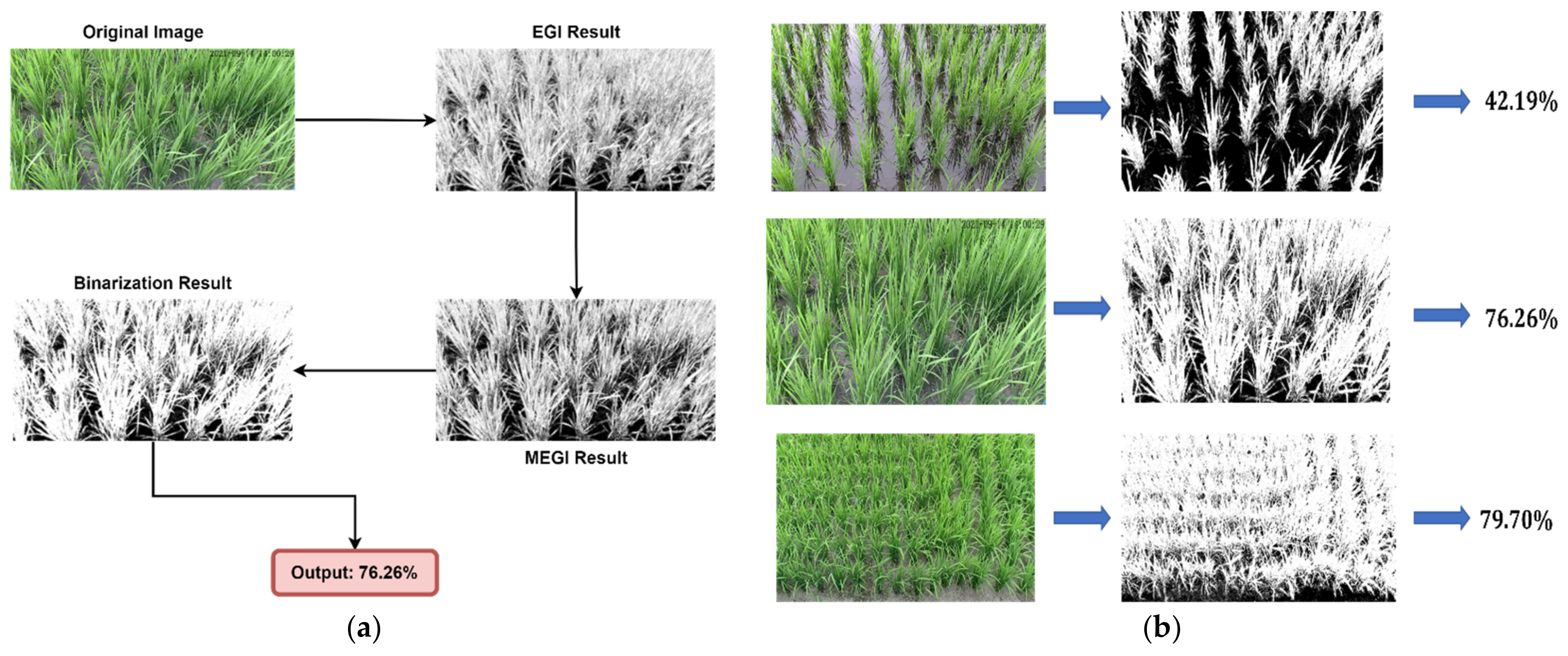
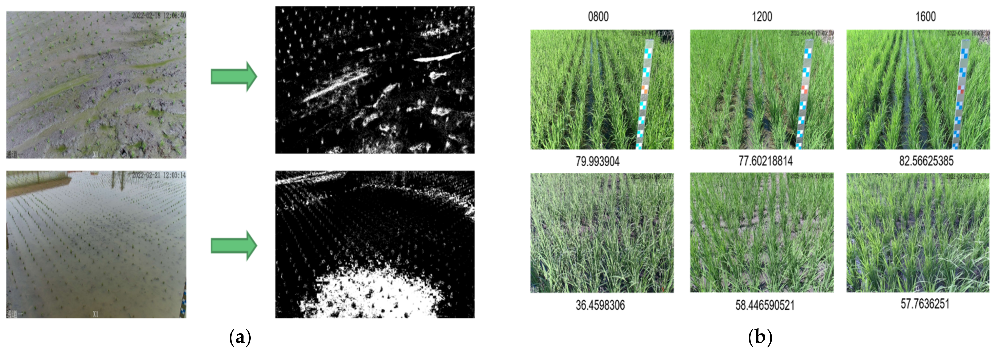
3.4.2. Green Coverage (GC) Rate
- The image is based on a large area of rice field and tries to avoid the non-field area.
- The image angle is based on the depression angle and tries to cover only the rice field area.
- Likely, the uneven coloration or partial brightness of the objects in the image will be caused by the intensity of the sunlight in the morning (sunrise) and the evening (sunset). To reduce the impact of the natural environment on the photos, we chose the images taken between 8:00 am and 4:00 pm.
3.4.3. Excess Green Index (EGI) and Modified EGI
3.4.4. Binarization and CC Rate Calculation
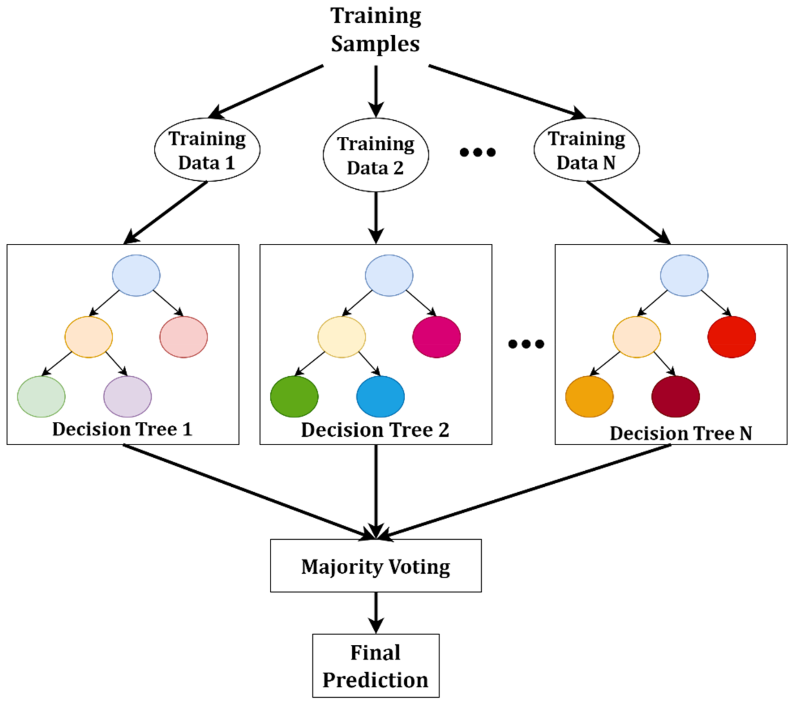
3.5. RF-Based ML Classification Model
3.6. Data Labelling
4. Experiment and Results
4.1. Image Recognition Using Instance Segmentation Model
4.2. Image Processing-Based Height Calculation
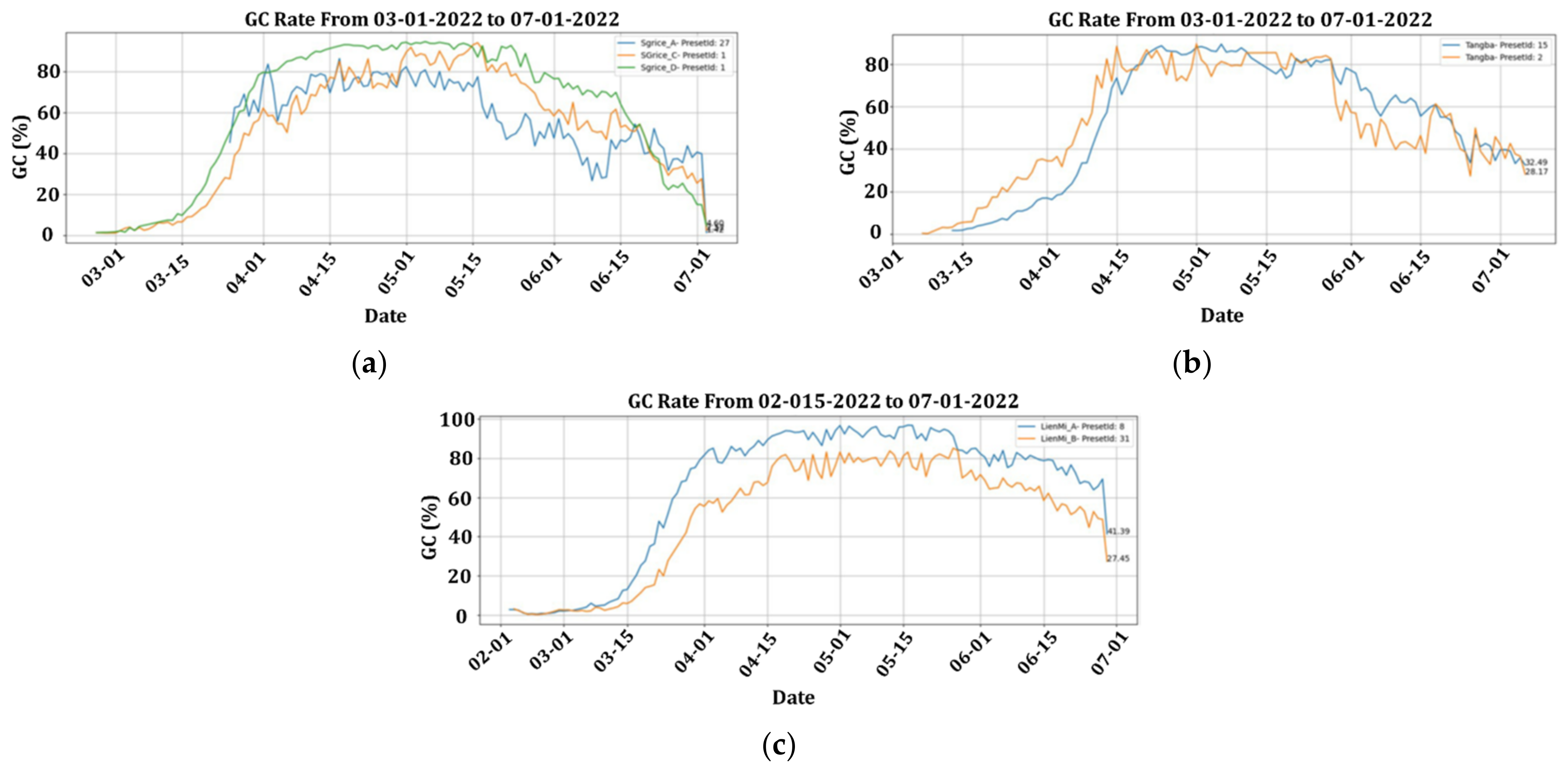
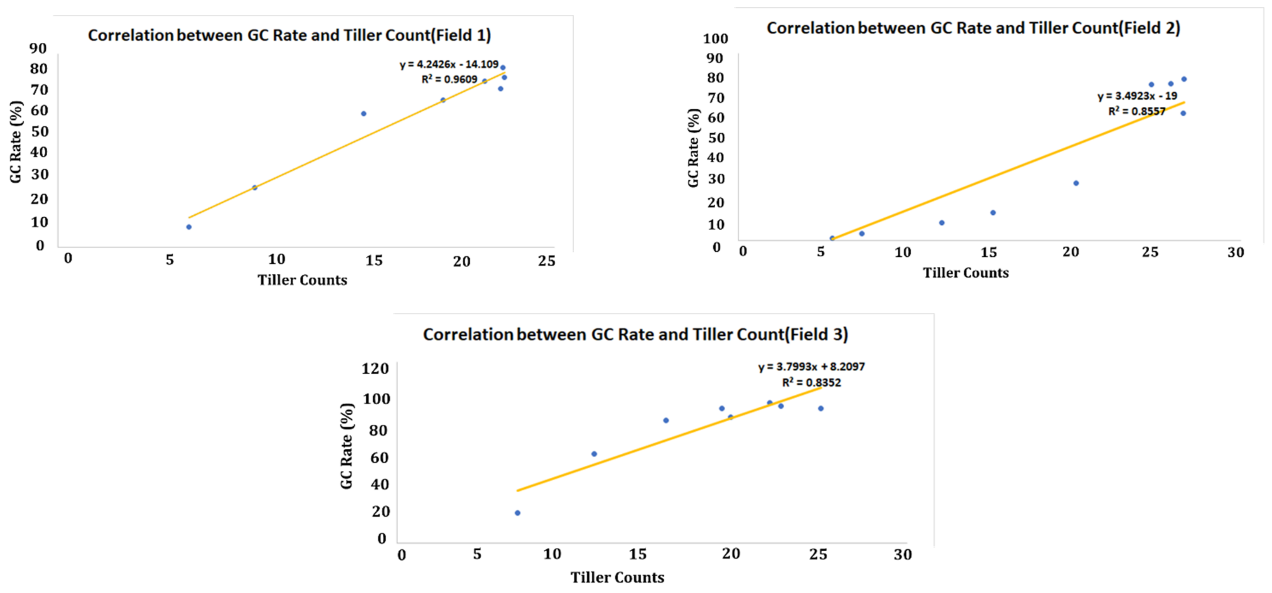
4.3. Green Coverage (GC) Rate
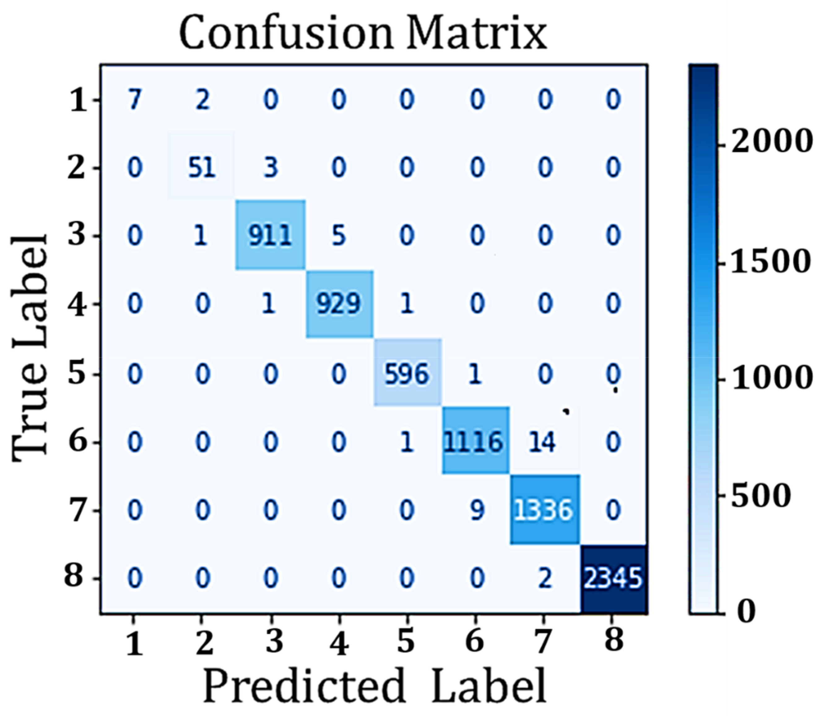
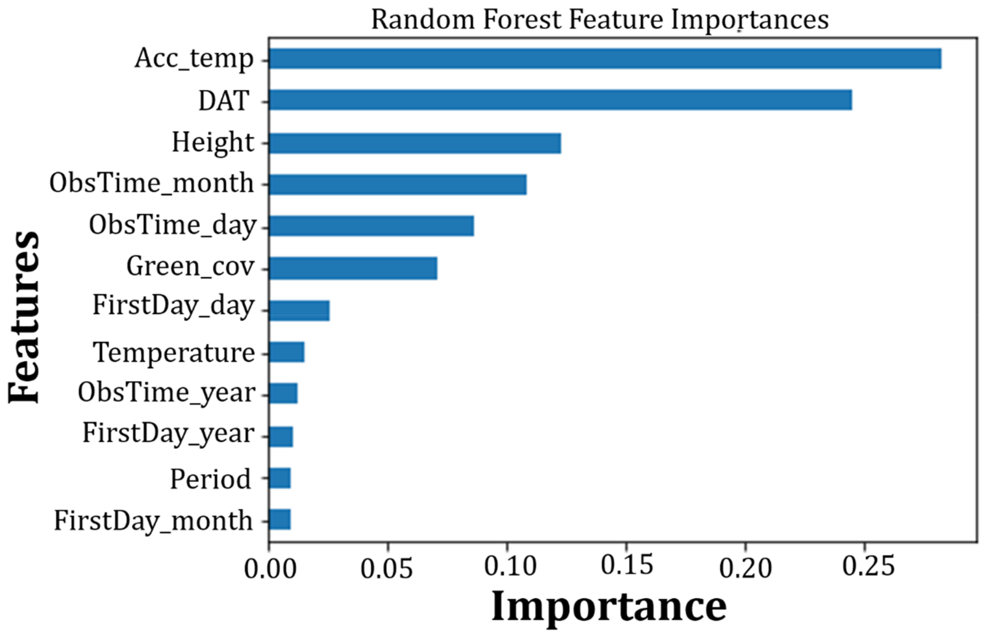
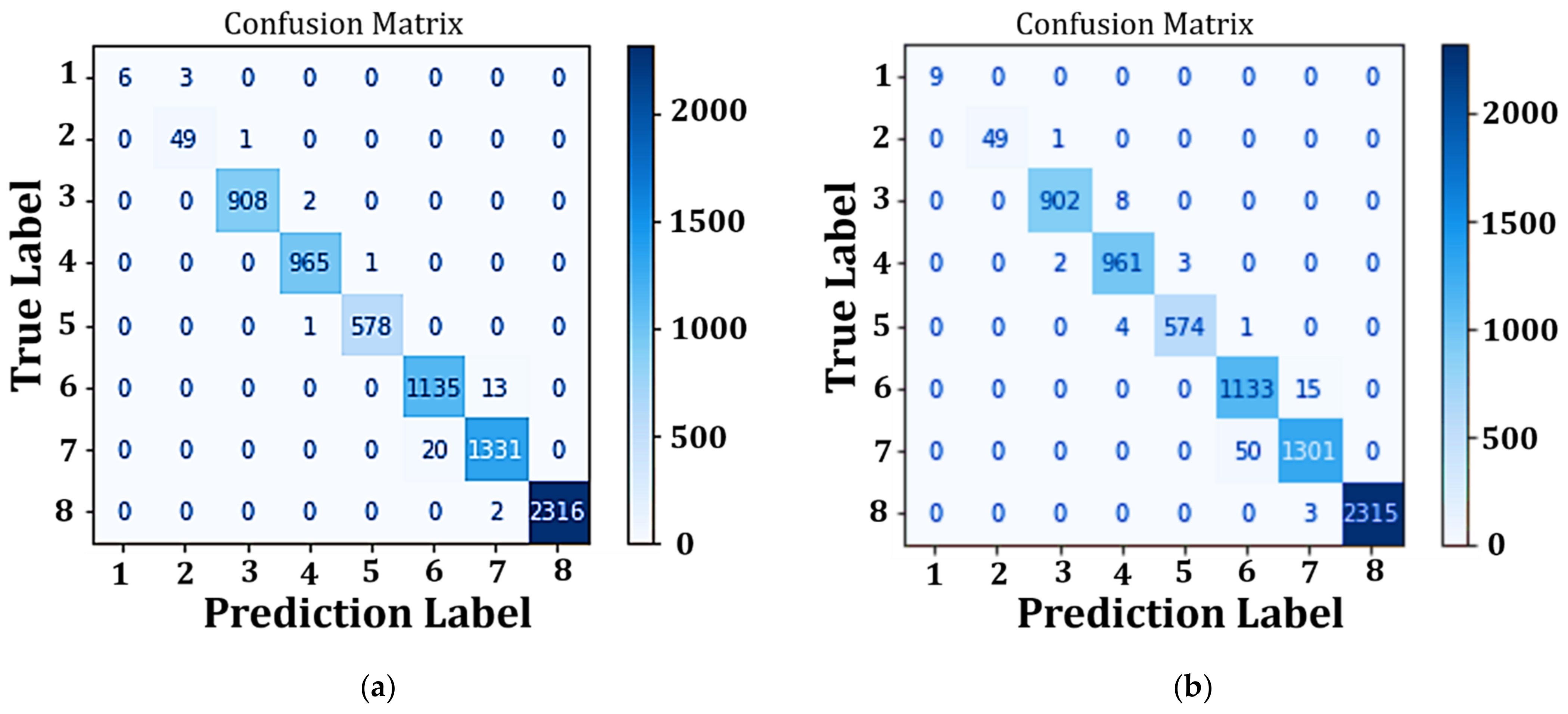
4.4. Performance Analysis of Classification Model
5. Conclusions and Future Works
Author Contributions
Funding
Institutional Review Board Statement
Informed Consent Statement
Data Availability Statement
Conflicts of Interest
References
- Bhat, S.A.; Huang, N.-F.; Sofi, I.B.; Sultan, M. Agriculture-Food Supply Chain Management Based on Blockchain and IoT: A Narrative on Enterprise Blockchain Interoperability. Agriculture 2021, 12, 40. [Google Scholar] [CrossRef]
- Hsing, Y. Rice in taiwan. In Encyclopaedia of the History of Science, Technology, and Medicine in Non-Western Cultures; Springer: Berlin/Heidelberg, Germany, 2016; pp. 3769–3772. [Google Scholar]
- Rice Can be Harvested Several Times a Year. Available online: https://kmweb.coa.gov.tw/knowledge_view.php?id=167 (accessed on 15 August 2022).
- Ramadhani, F.; Pullanagari, R.; Kereszturi, G.; Procter, J. Mapping a cloud-free rice growth stages using the integration of proba-v and sentinel-1 and its temporal correlation with sub-district statistics. Remote Sens. 2021, 13, 1498. [Google Scholar] [CrossRef]
- Production and Sales History Agricultural Products Production Process Taiwan Good Agricultural Practice (TGAP)-Rice-Paddy. Available online: https://www.afa.gov.tw/cht/index.php (accessed on 15 September 2022).
- Onyeneke, R.U.; Amadi, M.U.; Njoku, C.L.; Osuji, E.E. Climate Change Perception and Uptake of Climate-Smart Agriculture in Rice Production in Ebonyi State, Nigeria. Atmosphere 2021, 12, 1503. [Google Scholar] [CrossRef]
- Alfred, R.; Obit, J.H.; Chin, C.P.-Y.; Haviluddin, H.; Lim, Y. Towards paddy rice smart farming: A review on big data, machine learning, and rice production tasks. IEEE Access 2021, 9, 50358–50380. [Google Scholar] [CrossRef]
- Thakur, A.K.; Uphoff, N.T. How the system of rice intensification can contribute to climate-smart agriculture. Agron. J. 2017, 109, 1163–1182. [Google Scholar] [CrossRef]
- Bhat, S.A.; Huang, N.-F. Big data and ai revolution in precision agriculture: Survey and challenges. IEEE Access 2021, 9, 110209–110222. [Google Scholar] [CrossRef]
- Bhat, S.A.; Huang, N.-F.; Hussain, I.; Bibi, F.; Sajjad, U.; Sultan, M.; Alsubaie, A.S.; Mahmoud, K.H. On the Classification of a Greenhouse Environment for a Rose Crop Based on AI-Based Surrogate Models. Sustainability 2021, 13, 12166. [Google Scholar] [CrossRef]
- Huang, T.-W.; Bhat, S.A.; Huang, N.-F.; Chang, C.-Y.; Chan, P.-C.; Elepano, A.R. Artificial intelligence-based real-time pineapple quality classification using acoustic spectroscopy. Agriculture 2022, 12, 129. [Google Scholar] [CrossRef]
- Muthusinghe, M.; Palliyaguru, S.; Weerakkody, W.; Saranga, A.H.; Rankothge, W. Towards smart farming: Accurate prediction of paddy harvest and rice demand. In Proceedings of the 2018 IEEE Region 10 Humanitarian Technology Conference (R10-HTC), Colombo, Sri Lanka, 6–8 December 2018; pp. 1–6. [Google Scholar]
- Nishantha, M.D.L.C.; Zhao, X.; Jeewani, D.C.; Bian, J.; Nie, X.; Weining, S. Direct comparison of β-glucan content in wild and cultivated barley. Int. J. Food Prop. 2018, 21, 2218–2228. [Google Scholar] [CrossRef] [Green Version]
- Vesali, F.; Omid, M.; Kaleita, A.; Mobli, H. Development of an android app to estimate chlorophyll content of corn leaves based on contact imaging. Comput. Electron. Agric. 2015, 116, 211–220. [Google Scholar] [CrossRef]
- Haw, C.L.; Ismail, W.I.W.; Kairunniza-Bejo, S.; Putih, A.; Shamshiri, R. Colour vision to determine paddy maturity. Int. J. Agric. Biol. Eng. 2014, 7, 55–63. [Google Scholar]
- Lee, K.-J.; Lee, B.-W. Estimating canopy cover from color digital camera image of rice field. J. Crop Sci. Biotechnol. 2011, 14, 151–155. [Google Scholar] [CrossRef]
- Lee, K.-J.; Lee, B.-W. Estimation of rice growth and nitrogen nutrition status using color digital camera image analysis. Eur. J. Agron. 2013, 48, 57–65. [Google Scholar] [CrossRef]
- Zainuddin, Z.; Manjang, S.; Wijaya, A.S. Rice farming age detection use drone based on SVM histogram image classification. In Journal of Physics: Conference Series; IOP Publishing: Bristol, UK, 2019; p. 092001. [Google Scholar]
- Zhang, Y.; Xiao, D.; Liu, Y. Automatic Identification Algorithm of the Rice Tiller Period Based on PCA and SVM. IEEE Access 2021, 9, 86843–86854. [Google Scholar] [CrossRef]
- Ikasari, I.H.; Ayumi, V.; Fanany, M.I.; Mulyono, S. Multiple regularizations deep learning for paddy growth stages classification from LANDSAT-8. In Proceedings of the 2016 International Conference on Advanced Computer Science and Information Systems (ICACSIS), Malang, Indonesia, 15–16 October 2016; pp. 512–517. [Google Scholar]
- Murata, K.; Ito, A.; Takahashi, Y.; Hatano, H. A study on growth stage classification of paddy rice by cnn using ndvi images. In Proceedings of the 2019 Cybersecurity and Cyberforensics Conference (CCC), Melbourne, Australia, 8–9 May 2019; pp. 85–90. [Google Scholar]
- Wu, Y.; Kirillov, A.; Massa, F.; Lo, W.; Girshick, R. Detectron2 [WWW Document]. 2019. Available online: https://github.com/facebookresearch/detectron2 (accessed on 3 March 2021).
- Xie, S.; Girshick, R.; Dollár, P.; Tu, Z.; He, K. Aggregated residual transformations for deep neural networks. In Proceedings of the IEEE Conference on Computer Vision and Pattern Recognition, Honolulu, HI, USA, 21–26 July 2017; pp. 1492–1500. [Google Scholar]
- He, K.; Gkioxari, G.; Dollár, P.; Girshick, R. Mask r-cnn. In Proceedings of the IEEE International Conference on Computer Vision, Venice, Italy, 22–29 October 2017; pp. 2961–2969. [Google Scholar]
- Abdulla, W. Splash of color: Instance segmentation with mask r-cnn and tensorflow. Matterport Eng. Techblog 2018. Available online: https://engineering.matterport.com/splash-of-color-instance-segmentation-with-mask-r-cnn-and-tensorflow-7c761e238b46/ (accessed on 3 November 2022).
- Nthu Smart Farming Platform. Available online: https://nthu-smart-farming.kits.tw/ (accessed on 5 November 2022).
- Paul, A.; Mukherjee, D.P.; Das, P.; Gangopadhyay, A.; Chintha, A.R.; Kundu, S. Improved random forest for classification. IEEE Trans. Image Process. 2018, 27, 4012–4024. [Google Scholar] [CrossRef] [PubMed]
- Chiu, M.-C.; Yan, W.-M.; Bhat, S.A.; Huang, N.-F. Development of smart aquaculture farm management system using IoT and AI-based surrogate models. J. Agric. Food Res. 2022, 9, 100357. [Google Scholar] [CrossRef]
- Charbuty, B.; Abdulazeez, A. Classification based on decision tree algorithm for machine learning. J. Appl. Sci. Technol. Trends 2021, 2, 20–28. [Google Scholar] [CrossRef]
- Géron, A. Hands-On Machine Learning with Scikit-Learn, Keras, and TensorFlow; O’Reilly Media, Inc.: Sebastopol, CA, USA, 2022. [Google Scholar]


| Stage | Phase | Selection |
|---|---|---|
| Transplantation | Vegetative | Yes |
| Early Tillering | Yes | |
| Peak Tillering | Yes | |
| Late Tillering | Yes | |
| Panicle Initiation | Reproductive | Yes |
| Booting | Yes | |
| Heading | Yes | |
| Milk | Ripening | Yes |
| Dough | Yes | |
| Yellow Ripening | Yes | |
| Mature | Yes |
| Name | lr Sched | Train Time (s/iter) | Inference Time (s/im) | Train mem (GB) | Box AP | Mask AP | Model Id |
|---|---|---|---|---|---|---|---|
| R50-C4 | 1× | 0.584 | 0.110 | 5.2 | 36.8 | 32.2 | 137259246 |
| R50-DC5 | 1× | 0.471 | 0.076 | 6.5 | 38.3 | 34.2 | 137260150 |
| R50-FPN | 1× | 0.261 | 0.043 | 3.4 | 38.6 | 35.2 | 137260431 |
| R50-C4 | 3× | 0.575 | 0.111 | 5.2 | 39.8 | 34.4 | 137849525 |
| R50-DC5 | 3× | 0.470 | 0.076 | 6.5 | 40.0 | 35.9 | 137849551 |
| R50-FPN | 3× | 0.261 | 0.043 | 3.4 | 41.0 | 37.2 | 137849600 |
| R101-C4 | 3× | 0.652 | 0.145 | 6.3 | 42.6 | 36.7 | 138363239 |
| R101-DC5 | 3× | 0.545 | 0.092 | 7.6 | 41.9 | 37.3 | 138363294 |
| R101-FPN | 3× | 0.340 | 0.056 | 4.6 | 42.9 | 38.6 | 138205316 |
| X101-FPN | 3× | 0.690 | 0.103 | 7.2 | 44.3 | 39.5 | 139653917 |
| Field | Farming Period | Data Count | Stages | Data Count | Stages | Data Count |
|---|---|---|---|---|---|---|
| 1 | 1, 2 | 25,140 | 1 | 36 | 5 | 3865 |
| 2 | 1, 2 | 600 | 2 | 200 | 6 | 4592 |
| 3 | 1 | 3584 | 3 | 2316 | 7 | 5406 |
| 4 | 3638 | 8 | 9271 | |||
| Total | 29,324 | |||||
| Training Features | Definition |
|---|---|
| green_cov | GC rate calculated from the image, outputted from GC block |
| period | Farming period (first or second), 1 and 2 are used to represent these growing periods |
| FirstDay_day | The day of transplantation date (e.g., 2022/03/04, day = 4) |
| FirstDay_month | The month of transplantation date (e.g., 2022/03/19, month = 3) |
| FirstDay_year | The year of transplantation data ((e.g., 2022/03/04, year = 2022)) |
| ObsTime_day | The day of the input image’s observation date (e.g., 2022/03/19, day = 4) |
| ObsTime_month | The month of input image’s observation month (e.g., 2022/03/19, month = 3) |
| ObsTime_year | The year of input image’s observation year (e.g., 2022/03/19, year = 2022) |
| DAT | Days after transplantation (Observation Date-First Day (Date) = DAT) |
| Temperature (°C) | Air temperature of the day collected by installed sensors |
| acc_temp | Accumulated temperature, T−10 = Effective accumulated temperature of the day, Start summing up from the transplantation day till the observation day |
| height | Output (height) from height calculation block |
| Growth Stage | Code | Growth Stage | Code |
|---|---|---|---|
| Transplantation Stage | 1 | Panicle Initiation Stage | 5 |
| Early Tillering Stage | 2 | Booting Stage | 6 |
| Peak Tillering Stage | 3 | Heading Stage | 7 |
| Late Tillering Stage | 4 | Ripening Stage | 8 |
| Evaluation Type | Score | |||
|---|---|---|---|---|
| AP | AP50 | AP75 | AR | |
| Bounding Box | 0.559 | 0.780 | 0.671 | 0.613 |
| Segmentation | 0.506 | 0.780 | 0.660 | 0.539 |
| Date. | 9/3 | 9/10 | 9/17 | 9/24 | 10/1 | 10/8 | 10/15 | Average |
|---|---|---|---|---|---|---|---|---|
| Height Calculation | 47.8 | 62.7 | 75.5 | 84.7 | 87.6 | 82.3 | 97.1 | |
| Ground Truth | 48.0 | 60.4 | 75.4 | 85.9 | 90.5 | 97.8 | 106.0 | |
| Difference | −0.2 | +2.3 | +1.2 | −1.2 | −2.9 | −5.5 | −8.9 | 3.0 |
| Error Rate | −0.42(%) | +3.81(%) | +0.13(%) | −1.40(%) | −3.20(%) | −5.62(%) | −8.40(%) | 3.28(%) |
| Date | 3/17 | 3/25 | 4/1 | 4/8 | 4/15 | 4/22 | 4/29 | 5/6 | 5/13 | 5/20 | 5/27 | 6/3 | 6/10 | 6/17 | Average |
|---|---|---|---|---|---|---|---|---|---|---|---|---|---|---|---|
| Height Calculation Result | 17.38 | 32.32 | 37.58 | 41.30 | 46.56 | 57.84 | 67.26 | 69.99 | 76.51 | 81.57 | 82.32 | 92.33 | 94.95 | 95.01 | |
| Ground Truth | 18.38 | 33.88 | 41.38 | 55.88 | 56.38 | 58.75 | 67.88 | 69.75 | 71.75 | 78.00 | 81.38 | 83.38 | 94.00 | 103.38 | |
| Difference | −1.00 | −1.59 | −3.79 | −14.58 | −9.82 | −0.91 | −0.62 | 0.24 | 4.75 | 3.57 | 0.84 | 8.96 | 0.95 | −8.33 | −1.52 |
| Error Rate | 5.42% | 4.70% | 9.17% | 26.09% | 17.42% | 1.55% | 0.91% | 0.34% | 6.63% | 4.58% | 1.16% | 10.74% | 1.01% | 8.06% | 6.98% |
| Date | 3/12 | 3/19 | 3/26 | 4/1 | 4/9 | 4/16 | 4/23 | 5/7 | 5/28 | 6/3 | Average |
|---|---|---|---|---|---|---|---|---|---|---|---|
| Height Calculation Result | 41.88 | 45.35 | 52.76 | 57.52 | 63.00 | 68.04 | 78.53 | 86.39 | 105.03 | 123.26 | |
| Ground Truth | 10.3 | 18 | 26.85 | 33.6 | 38.1 | 48.9 | 58.8 | 71.2 | 100.8 | 103.9 | |
| Difference | 31.58 | 27.35 | 25.91 | 23.92 | 24.90 | 19.14 | 19.73 | 15.19 | 4.23 | 19.36 | 21.13 |
| Error Rate | 306.60% | 151.94% | 96.50% | 71.19% | 65.35% | 39.14% | 33.55% | 21.33% | 4.19% | 18.63% | 80.84% |
| Field | Depression Angle | Distance from Camera to Chessboard (m) | Chess Height above Ground (m) | Camera Height (m) |
|---|---|---|---|---|
| 1 | 23 | 1.2 | 0.6 | 1.0689 |
| 2 | 35 | 1.45 | 0.6 | 1.4317 |
| 3 | 50 | 1.596 | 0.6 | 1.8228 |
| Accuracy | Macro F1-Score | Macro Precision | Macro Recall | |
|---|---|---|---|---|
| Random Forest (baseline) | 0.99454 | 0.97337 | 0.98883 | 0.96138 |
| Stage | Precision | Recall | F1-Score | Total |
|---|---|---|---|---|
| 1 | 1.00000 | 0.77778 | 0.87500 | 9 |
| 2 | 0.94444 | 0.94444 | 0.94444 | 54 |
| 3 | 0.99563 | 0.99346 | 0.99454 | 917 |
| 4 | 0.99465 | 0.99785 | 0.99625 | 931 |
| 5 | 0.99666 | 0.99832 | 0.99749 | 597 |
| 6 | 0.99112 | 0.98674 | 0.98892 | 1131 |
| 7 | 0.98817 | 0.99331 | 0.99073 | 1345 |
| 8 | 1.00000 | 0.99915 | 0.99957 | 2347 |
| Stage | Before | RandomOverSampler | SMOTE-ENN | Stage | Before | RandomOverSampler | SMOTE-ENN |
|---|---|---|---|---|---|---|---|
| 1 | 27 | 6953 | 6951 | 5 | 1737 | 6953 | 6932 |
| 2 | 150 | 6953 | 6923 | 6 | 3444 | 6953 | 6699 |
| 3 | 2728 | 6953 | 6922 | 7 | 4055 | 6953 | 6710 |
| 4 | 2899 | 6953 | 6884 | 8 | 6953 | 6953 | 6931 |
| Model | Accuracy | Macro F1-Score | Macro Precision | Macro Recall |
|---|---|---|---|---|
| RF (Less Features) | 0.99018 | 0.95888 | 0.96949 | 0.94932 |
| RF (RandomOverSampler) | 0.99373 | 0.96551 | 0.98805 | 0.95141 |
| RF (SMOTE-ENN) | 0.98772 | 0.98653 | 0.98518 | 0.98802 |
| Model | Accuracy | Macro F1-Score | Macro Precision | Macro Recall |
|---|---|---|---|---|
| RF (SMOTE-ENN) | 0.98772 | 0.98653 | 0.98518 | 0.98802 |
| KNN | 0.96576 | 0.93469 | 0.95007 | 0.92945 |
| SVC | 0.97313 | 0.96515 | 0.95547 | 0.97744 |
| AdaBoost | 0.43609 | 0.32895 | 0.25549 | 0.47271 |
| GaussianNB | 0.83317 | 0.74009 | 0.71020 | 0.83983 |
| Logistic Regression | 0.86782 | 0.80107 | 0.76618 | 0.87496 |
Publisher’s Note: MDPI stays neutral with regard to jurisdictional claims in published maps and institutional affiliations. |
© 2022 by the authors. Licensee MDPI, Basel, Switzerland. This article is an open access article distributed under the terms and conditions of the Creative Commons Attribution (CC BY) license (https://creativecommons.org/licenses/by/4.0/).
Share and Cite
Sheng, R.T.-C.; Huang, Y.-H.; Chan, P.-C.; Bhat, S.A.; Wu, Y.-C.; Huang, N.-F. Rice Growth Stage Classification via RF-Based Machine Learning and Image Processing. Agriculture 2022, 12, 2137. https://doi.org/10.3390/agriculture12122137
Sheng RT-C, Huang Y-H, Chan P-C, Bhat SA, Wu Y-C, Huang N-F. Rice Growth Stage Classification via RF-Based Machine Learning and Image Processing. Agriculture. 2022; 12(12):2137. https://doi.org/10.3390/agriculture12122137
Chicago/Turabian StyleSheng, Rodney Tai-Chu, Yu-Hsiang Huang, Pin-Cheng Chan, Showkat Ahmad Bhat, Yi-Chien Wu, and Nen-Fu Huang. 2022. "Rice Growth Stage Classification via RF-Based Machine Learning and Image Processing" Agriculture 12, no. 12: 2137. https://doi.org/10.3390/agriculture12122137