Deep-Learning Temporal Predictor via Bidirectional Self-Attentive Encoder–Decoder Framework for IOT-Based Environmental Sensing in Intelligent Greenhouse

Abstract

Smart agricultural greenhouses provide well-controlled conditions for crop cultivation but require accurate prediction of environmental factors to ensure ideal crop growth and management efficiency. Due to the limitations of existing predictors in dealing with massive, nonlinear, and dynamic temporal data, this study proposes a bidirectional self-attentive encoder–decoder framework (BEDA) to construct the long-time predictor for multiple environmental factors with high nonlinearity and noise in a smart greenhouse. Firstly, the original data are denoised by wavelet threshold filter and pretreatment operations. Secondly, the bidirectional long short-term-memory is selected as the fundamental unit to extract time-serial features. Then, the multi-head self-attention mechanism is incorporated into the encoder–decoder framework to improve the prediction performance. Experimental investigations are conducted in a practical greenhouse to accurately predict indoor environmental factors (temperature, humidity, and CO₂) from noisy IoT-based sensors. The best model for all datasets was the proposed BEDA method, with the root mean square error of three factors’ prediction reduced to 2.726, 3.621, and 49.817, and with an R of 0.749 for temperature, 0.848 for humidity, and 0.8711 for CO₂ concentration, respectively. The experimental results show that the favorable prediction accuracy, robustness, and generalization of the proposed method make it suitable to more precisely manage greenhouses.

1. Introduction

With the rapidly growing demand of global population, modern agriculture has become an increasingly vital role in guaranteeing food production supply, ensuring social stability and safeguarding ecological environment sustainability all over the world. It is the important component of global trade economy which greatly contributes to job creation, income source, and gross domestic product of most countries. To provide healthy food to feed the population worldwide, smart agricultural greenhouses (SAG) utilize advanced intelligent information technologies to break through the limits of natural conditions by providing a stable and controllable environment for crop growing and planting management, which has recently become the significant solution to produce more with minimal socioeconomic and ecological loss from limited tillage and labor [1]. On basis of artificial intelligence [2], Internet of Things (IoT) [3], big data computing [4], 5G communication [5], blockchain [6], etc., the SAG systems record various environmental factors for real-time monitoring of crop growth status and soil/climate changes, which aims to optimize the crop production process and manage sustainable supply chain practices as efficiently and reasonably as possible. Based on many environmental data recorded intelligently in the greenhouse, SAG systems also gradually show ability in reforming the agricultural applications by enhancing the growth rate and yield, improving quality and safety of various crop production, and reducing human labor intensity.

Nevertheless, greenhouses are still susceptible to the atmospheric conditions, soil state, and other environmental factors such as humidity, air temperature, light intensity, carbon dioxide/Ozone concentrations, soil pH value, solar radiation, ultraviolet intensity, and rainfall, which directly affect crop growth and yield. Therefore, accurately evaluating infield environmental factors, and even further predicting future information, can generate more benefits for smart agricultural applications in both controlled greenhouses and large-scale farmlands [7]. Taking fruit planting in greenhouses as an example, efficient operation for optimum productivity requires a careful and comprehensive understanding of plentiful information about greenhouse indoor and outdoor environments, which are associated with various plant growth processes including photosynthesis, respiration, transpiration, phytohormone secretion, and so on. In addition, forecasting greenhouse environmental changes can provide intelligent field interventions to farmers with guidance about soil nutrients regulation, crop maturity cycle, harvesting operations, and disease/pest prevention.

Therefore, for enhancing resistance to potential risks and management efficiency in the agricultural industry, the technology development of environmental factor forecasting is indispensable in smart greenhouse systems. Particularly, it is extremely necessary to utilize the state-of-the-art mathematical models to efficiently assist in uplifting the prediction performance of intelligent systems in one way or another. Many studies have made many great efforts to accomplish the dynamic environmental prediction of modern greenhouses. Prediction algorithms are established through parameter estimation methods [8], statistic representative methods [9], shallow neural networks [10], and deep-learning models [11], to obtain professional future knowledge regarding the variation tendency of environmental conditions in IoT-based precision agricultural applications. Those attempts usually train predicting models using some current and historical data to extract representational features for maximization of profit and minimization of losses. Afterwards, these disciplinary models are applied to make informed decisions for various agronomic tasks in the designated agricultural scenes, which observably contributes to increasing crop production by more than 10 times, compared with open-environment cultivation.

However, the accurate prediction of environmental factors is a very complex nonlinear temporal issue affected by various internal and external variables, making it still challenging to forecast the future variation trends. Since the above algorithms are constructed for a particular application, their performance becomes degraded when operational conditions and datasets are changing over a long time. Additionally, thanks to high-frequency and large-scale sensing data stored by IoT systems, it becomes possible to analyze sensory data and discover new features for making accurate long-term predictions; however, subsequently, different environmental factors have complex nonlinear relationships with noisy interference, which makes it difficult for a single general model to predict different variables at the same time. To obtain an accurate system model for filtering, prediction, and control, some identification methods can used to achieve this objective [12,13,14,15,16] and to establish the mathematical models of dynamic systems from observation data [17,18,19,20,21,22,23], and other identification methods can be used to establish the prediction models and soft-sensor models for various purposes [24,25,26,27,28].

Internet of Things (IoT) technology combines interconnected devices and programs into a complete system that transfers data over the network without the need for human interaction. Through IoT technology, researchers can collect, store, and analyze huge amounts of data. These massive amounts of data are nonlinear, random, volatile, multidimensional, and contain noise. Existing microclimate and data-driven models have low prediction accuracy and make it difficult to achieve accurate medium- to long-term forecasts. Noise in the data is strongly random and the model is not learnable. This has resulted in poor prediction accuracy. Although deep-learning models have a strong learning capability, the presence of noise can lead to overfitting of the model to the noise in the training set. This overlearning affects the robustness of the model. The greenhouse environmental control process is one of high inertia and lag. Accurate and stable prediction of changes and advance control of the greenhouse environment can create a better growing environment for crops and improve crop yield and quality. Therefore, modeling the greenhouse environment is of practical importance.

To solve existing problems in environmental factor prediction, a bidirectional self-attentive encoder–decoder framework (BEDA) is proposed to construct the long-time predictor for multiple environmental factors with strong nonlinearity and noise. Firstly, to avoid the problem of overfitting the model caused by noise in the data and to improve the stability of the model, this paper uses wavelet threshold denoising to filter the greenhouse data obtained from the sensor side. Then, the bidirectional long short-term-memory (LSTM) are selected as the fundamental units to build the encoder–decoder framework due to their ability in automatic feature extraction. Finally, the multi-head self-attention is incorporated into the proposed framework to improve the predicting performance and model robustness, which also presents good generalization effect for different input time series data.

The rest of this article is organized as follows. In Section 2, related work is introduced. In Section 3, the diagram and detailed structure of the proposed model are presented. Section 4 presents the experimental details and analysis results. Finally, conclusions are drawn in Section 5.

2. Related Works

Modern greenhouse environments are complex, nonlinear, time series, strongly coupled, etc. To design a reasonable greenhouse environmental regulation scheme, an accurate predictive model of the environmental factors within the greenhouse is required. Many studies have integrated some advanced technologies and methods to accomplish the dynamic prediction for environmental factors. Currently, there are two main types of greenhouse environmental models: one is the mechanistic modeling method on basis of energy conservation equations and mass conservation equations, and the other is the data-driven analytic modeling method based on extracting significant features and mining trend rules from an amount of input data.

2.1. Microclimate Mechanistic Modeling

A mechanistic model is one in which there are physical relationships that can be expressed probabilistically by physical or mathematical equations. Microclimate mechanistic modeling is the process of modeling a system based on the mechanics of a greenhouse system, such as the physical or chemical patterns of change.

Bontsema [29] studied the rate of air exchange in greenhouses using physics by examining the outdoor temperature, wind speed, the difference between indoor and outdoor temperatures, and the opening condition of the actuators. Berrow [30] gives calculations for transpiration, photosynthesis net radiation, and water vapor exchange given by analyzing the changes in heat and water vapor produced by plants in transpiration and photosynthesis. Rasheed [31] built a simulation model of a multi-span greenhouse and used a transient system simulation program to simulate the greenhouse microenvironment.

There are numerous studies on mechanistic modeling of greenhouses, but mechanistic model parameters are difficult to assess. Many variables are affecting physical experiments in greenhouses, many mechanisms are not yet clear, and as the environment continues to change, the conservation of energy equation needs to change accordingly. The degree of difficulty in accurately characterizing the physical environment of greenhouse microclimates using mathematical expressions is high. Thus, there are limitations to the application of mechanistic modeling in greenhouse environmental prediction.

2.2. Data-Driven Analytic Modeling

In recent years, greenhouse environmental prediction methods based on data-driven analytic modeling theory have become popular among researchers. The data-driven analytic approach treats the greenhouse system as a black box and relies only on real data collected in the greenhouse to match the greenhouse system. Among them, machine-learning and deep-learning technologies are important methods to address the prediction of greenhouse environments. Yu [32] used the particle swarm optimization (PSO) algorithm to optimize the least squares support vector machine (LSSVM) under the condition of principal component analysis (PCA) to improve the precision and efficiency of temperature prediction. Machine-learning methods have a complete theoretical derivation process and procedural modeling steps. For smooth data, a more accurate model can be given for prediction; however, machine-learning methods require more human intervention and have low modeling accuracy. When the data contains noise, it can affect the convergence of the model training.

Similarly, artificial neural networks are widely used in greenhouse environmental prediction problems. For example, Linker [33] trained a neural network greenhouse model using data collected over two summer months in a small greenhouse, and achieved optimal CO₂ control in the greenhouse using neural network modeling by predicting temperature and CO₂ separately. Ferreira [34] proposes the use of radial basis function neural networks to model the internal air temperature of hydroponic greenhouses as a function of the external air temperature and solar radiation, as well as the internal relative humidity. Four [35] modeled the greenhouse dynamic process using an Elman recurrent neural network and closed-loop control using a multilayer feedforward neural network, using this cascade model of inverse neural networks and feedforward networks to model the dynamics of the temperature and humidity data. These shallow networks have nonlinear fitting capabilities, but their learning capacity is limited. It is difficult for them to cope with large amounts of temporal data, and this makes the accuracy and general predicting results in the long term difficult, and can be easily overfitted.

In recent years, deep-learning technology has made significant breakthroughs in areas such as speech recognition, computer vision [36,37], and sequence classification [38], and can also be seen as an effective tool for achieving time series prediction [39,40]. The aim is to simulate the human brain for automatic data analysis and data representation. Perez [41] proposed recurrent neural networks (RNN) to predict inside air temperature and relative humidity in the greenhouse. The inputs of the network are various environmental factors including temperature, relative humidity, solar radiation, and so on. The actuators state signals such as window opening are selected as the outputs to training the model. Song [42] predicts short-, medium-, and long-term changes in indoor humidity using a multidimensional LSTM neural network for multiple environmental variables inside and outside the greenhouse, with better results than RNN neural models. These models can automatically learn hidden feature information from the data and capture nonlinearities well. Compared to machine-learning methods and shallow neural networks, deep-learning networks perform better and are more widely used. However, these models remain a stacked network structure with a single model structure, little variation in model structure for different problems, variable performance in prediction accuracy, and poor model robustness.

In addition, other deep-learning frameworks, such as encoder–decoder and attention networks, have a wide range of applications in areas such as power and energy forecasting [43] and air quality forecasting [44]. The encoder–decoder approach has become a popular sequence-to-sequence (seq2seq) architecture due to its success in the field of machine translation. The encoder–decoder encodes the source data as a fixed-length vector. The decoder is then used to produce an output that effectively extracts time series features and transform features from the input data. It simulates the learning process of a person acquiring information, comprehending it to form a memory, and then retelling it through a session. Its encoder and decoder structure can be CNN, RNN, LSTM, and other networks, with flexible model structure and strong information extraction capability. However, as the encoder input lengthens, the previous information is overwritten by the later information, resulting in a loss of information. A fixed-length encoding vector between the encoder and decoder will not contain all the input sequence information. Attentional mechanisms become an integral part of neural networks [45]. It overcomes the problem of information loss due to fixed-length coding of encoder–decoders and mines features with attention to detail. These novel network models are not widely used in greenhouse environmental prediction.

Thereby, the greenhouse is a continuously operating system that is nonlinear, time series, strongly coupled, and has sensors that inevitably introduce noise when monitoring the greenhouse environment. This poses a major challenge in making accurate predictions about the greenhouse environment. Existing greenhouse environmental prediction models have a single structure, low prediction accuracy, and poor generalization capability. The performance of the prediction models varies widely for different greenhouse environmental factors and the models cannot be widely used in applications. To address these issues, this paper proposes a bidirectional self-attentive coding and decoding model.

3. Materials and Methods

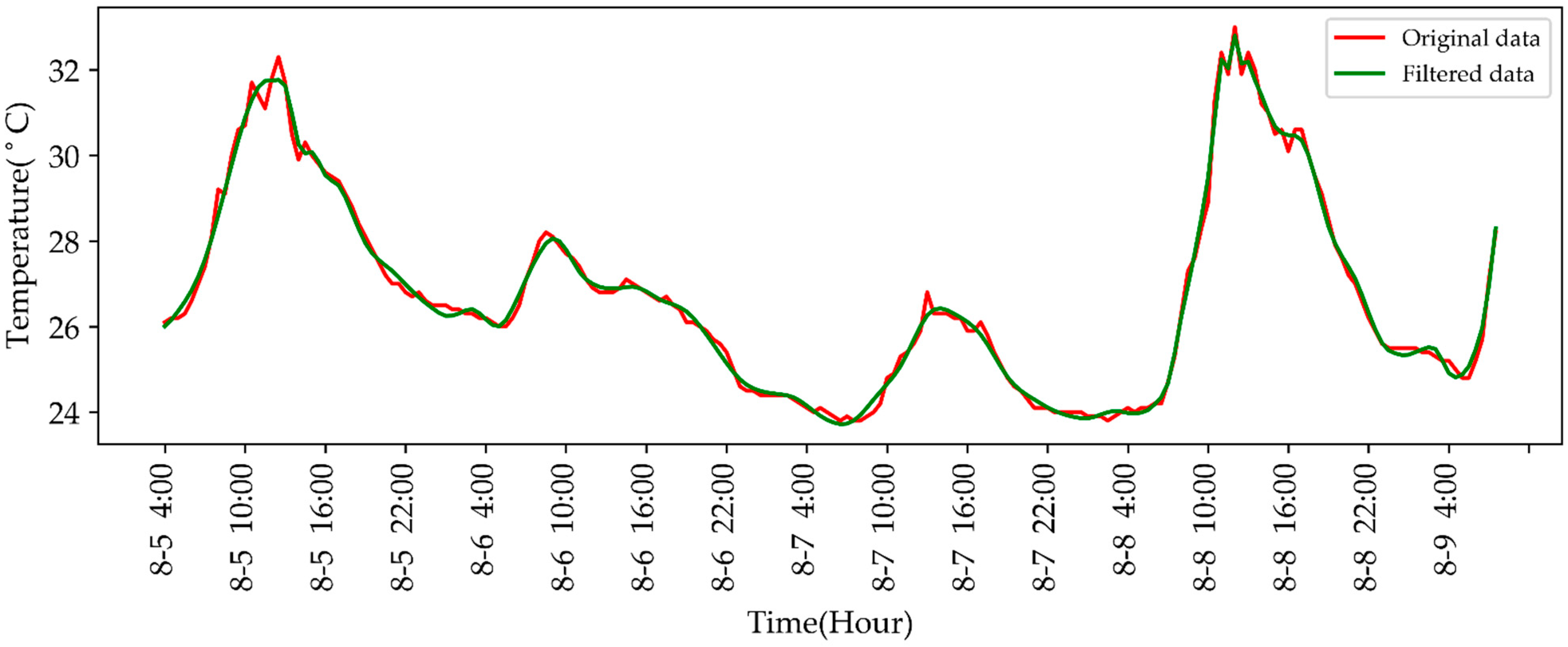
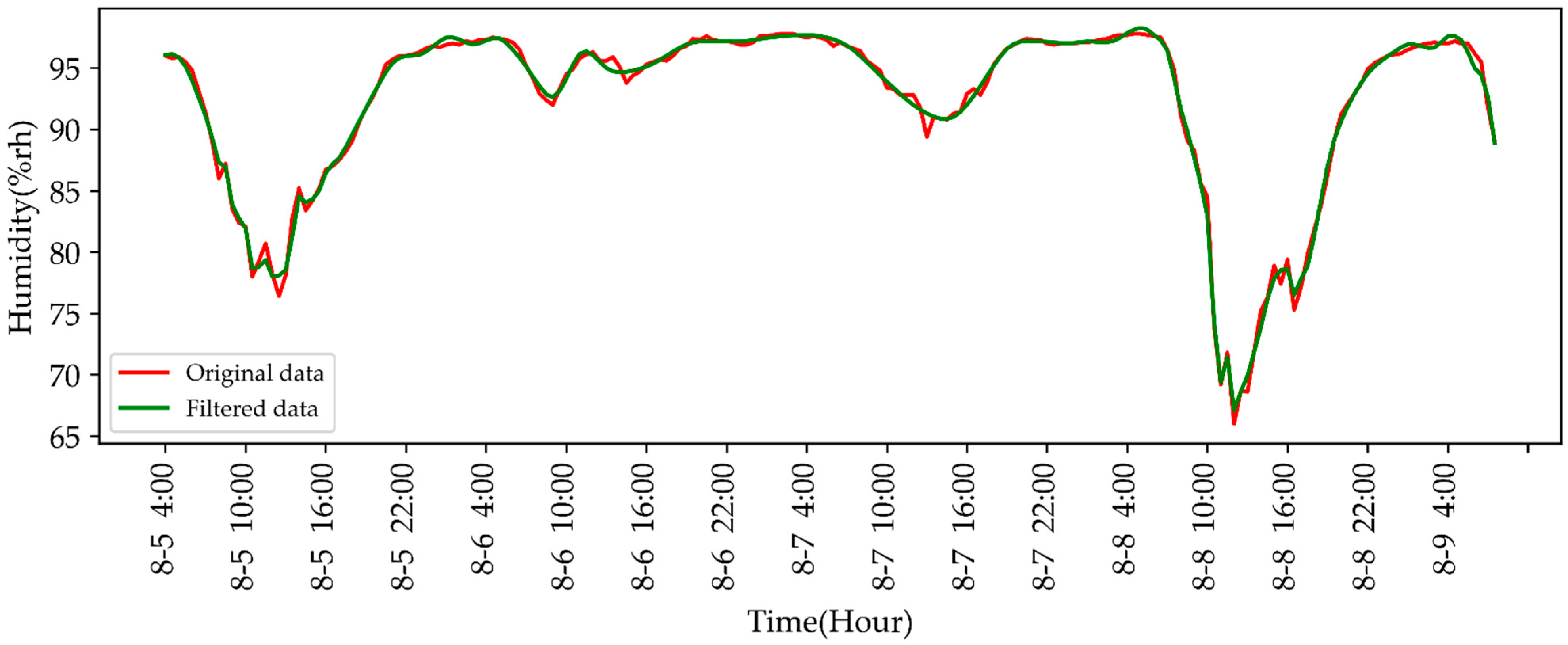
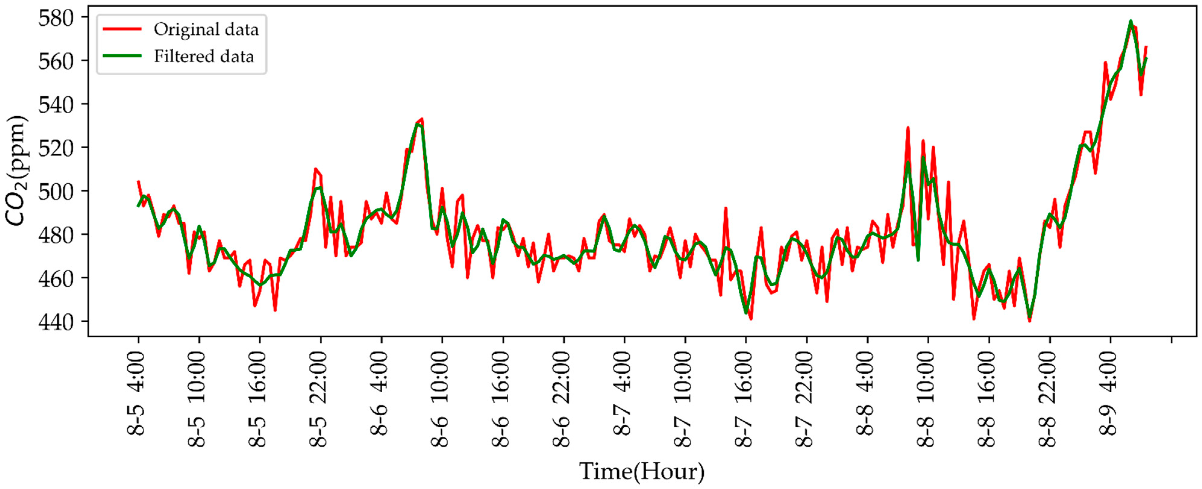
3.1. Wavelet Threshold Denoising

The data is affected by uncertainties in the acquisition process, such as the environment and sensors, resulting in a large amount of noise in the collected data while containing complex regular information, and the data usually shows strong randomness and strong nonlinearity [46,47]. If noisy data is analyzed directly, the results can be extremely distorted, so it is necessary to preprocess the data and analyze it to obtain an approximation of the true value of the data.

The discrete wavelet transform is a decomposition process. Assume that the number of decomposition layers is N, the mother wavelet function is $\eta (t)$, and the parent wavelet function is $\psi (t)$. The mother wavelet function and the parent wavelet function are orthogonal to each other, and the set obtained by applying the scale and translation transformations to them is the wavelet basis:

$${\eta }_{k,h}(t)=2^{\frac{k}{2}}\eta (2^{k}t-h)$$

(1)

$${\psi }_{k,h}(t)=2^{\frac{k}{2}}\psi (2^{k}t-h)$$

(2)

where $k\in R;k\ne 0$ is the scaling factor; $h\in R$ is the translation factor. The number of scale and translation transforms is determined by the length of the sequence and the number of decomposition layers. The original sequence $S(t)$ can be expressed as

$$S(t)={\displaystyle \sum _{h=1}^T{a}_{k,h}}{\psi }_{k,h}(t)+{\displaystyle \sum _{k=1}^N{\displaystyle \sum _{h=1}^T{d}_{k,h}{\eta }_{k,h}(t)}}=A_N+D_1+D_2+\cdots +D_i, i=1,2,\cdots ,N$$

(3)

where $T$ is the length of the original sequence; $a_{k,h}$ is the low-frequency component with a scale factor of $k$ and a translation factor of $h$; $d_{k,h}$ is the high-frequency component. The set of all low-frequency components in each layer decomposition is $A_i$, and the set of all high-frequency components is $D_i$. Decomposition of the low-frequency component of the previous layer occurs to obtain the high-frequency component of the next layer, i.e., $A_i=A_{i+1}+D_{i+1}$.

Once the components corresponding to the wavelet decomposition have been obtained, the noise is smoothed by selecting a suitable threshold $\upsilon$.

$$\sigma =\frac{median(D_i)}{0.6745}$$

(4)

$$\gamma =\sigma \sqrt{2\ln T}$$

(5)

$$\upsilon ={\lambda }_i\gamma$$

(6)

$$D_i{}^{\prime }=\{\begin{array}{ll}\left[\mathrm{sign}\left(D_{i,t}\right)\right](|D_{i,t}|-\upsilon )& \left|D_{i,t}\right|\ge \upsilon \\ 0& \left|D_{i,t}\right|<\upsilon \end{array}$$

(7)

where ${\lambda }_i$ is a scaling factor, and ${\lambda }_i\in (0,1) i=1,\cdots ,N$; $\sigma$ is the variance of the noise estimate; $median()$ is the median of the smoothed series; 0.6745 is the standard variance adjustment factor for Gaussian noise; $\gamma$ is the estimated threshold. After data reconstruction the filtered sequence is obtained as follows:

$$M(t)=A_N+D_1{}^{\prime }+D_2{}^{\prime }+\cdots +D_i{}^{\prime }, i=1,2,\cdots ,N$$

(8)

where $D_i{}^{\prime }$ indicates the high-frequency component after noise removal. The estimated true value $M(t)$ obtained retains the useful information in the original data $S(t)$, and the proportion of noise $M(t)$ is substantially reduced.

After wavelet threshold denoising, the filtered data is normalized and sliding windowed. The denoised data is normalized to improve the convergence speed and accuracy of the model.

$$X_s=\frac{X-\min (X)}{\max (X)-\min (X)}$$

(9)

The data is then processed by sliding window segmentation to divide the data into dimensions suitable for model input. The data window slides as shown in Figure 1.

The model input length is n and the prediction length is $\tau$. The window length is $n+\tau$ and the sliding step is 1. In the experiments, $n$ = 24 and $\tau$ = 24 are set.

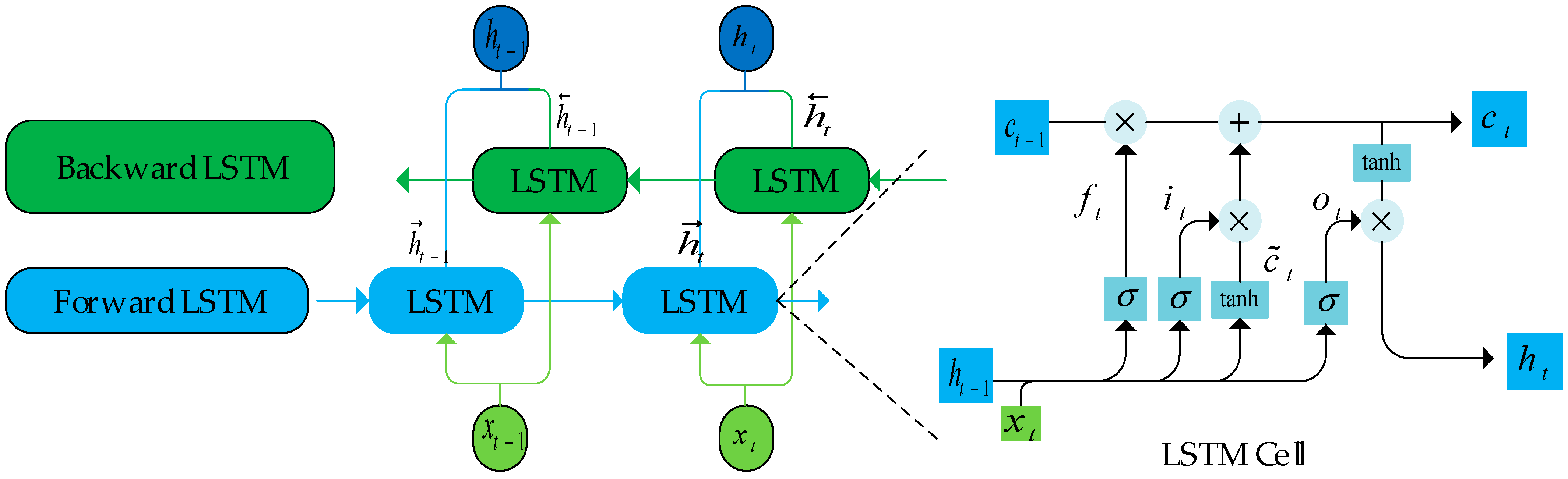
3.2. Bidirectional LSTM Unit

Bidirectional long short-term memory (BiLSTM) is a bidirectional version of LSTM, which is a combination of forwarding LSTM and backward LSTM. BiLSTM is capable of mining the laws that are difficult to resolve by LSTM, showing very good performance for complex classification and regression problems, and can make up for the shortcomings of one-way LSTM. The unidirectional LSTM network is to input the time series vectors in sequential order to obtain the prediction results. In real life, the information at the current moment is not only related to the previous information but may also have some relationship with the future information. The network structure of BiLSTM is shown in Figure 2.

The BiLSTM consists of two independent LSTM layers: the forward LSTM and the backward LSTM. The forward LSTM is computed in chronological order, while the reverse LSTM reverses the input sequence and computes it in reverse order. During training, the forward LSTM and reverse LSTM networks are independent of each other and have no interactions. Therefore, BiLSTM can better establish the correlation between time series internally. Among them, the forward propagation process of the LSTM cell is as follows:

$$f_t=\sigma \left(w_f\left[x_t;h_{t-1}\right]+b_f\right)$$

(10)

$$i_t=\sigma \left(w_i\left[x_t;h_{t-1}\right]+b_i\right)$$

(11)

$${\tilde{c}}_t=\sigma \left(w_c\left[x_t;h_{t-1}\right]+b_c\right)$$

(12)

$$c_t=f_t\times c_{t-1}+i_t\times {\tilde{c}}_t$$

(13)

$$o_t=\sigma \left(w_o\left[x_t;h_{t-1}\right]+b_o\right)$$

(14)

$$h_t=o_t\times \tanh (c_t)$$

(15)

where $f_t$ is the forget gate, $i_t$ is the input gate, $o_t$ is the output gated, $h_{t-1}$ is the hidden state of the previous cell, $c_{t-1}$ is the previous cell state, ${\tilde{c}}_t$ is a candidate for cell state, $c_t$ is the new cell content, $x_t$ is the input value at the current moment, $\sigma$ is the sigmoid activation function, $\tanh$ is the hyperbolic tangent activation function, $[;]$ is the collocation of elements, $\times$ is the multiplication between elements, $w_f$,$w_i$,$w_c$,$w_o$,$b_f$,$b_i$,$b_c$, and $b_o$ is the parameter to be learned.

The input of the forward LSTM is input in sequence order, and the final result is $[{\overrightarrow{h}}_1,{\overrightarrow{h}}_2,\cdots ,{\overrightarrow{h}}_t]$. The backward LSTM is the same process as the forward LSTM, except that the order of the input sequences is different. Eventually, the output of the reverse LSTM is $[{\overleftarrow{h}}_1,{\overleftarrow{h}}_2,\cdots ,{\overleftarrow{h}}_t]$. The final output of the BiLSTM network is as follows:

$$[h_1,h_2,\cdots ,h_t]=\left[[{\overrightarrow{h}}_1;{\overleftarrow{h}}_1],[{\overrightarrow{h}}_2;{\overleftarrow{h}}_2],\cdots ,[{\overrightarrow{h}}_t;{\overleftarrow{h}}_t]\right]$$

(16)

where $[;]$ can be concatenation, summation, and multiplication of corresponding elements. BiLSTM enhances the interaction of sequence datasets by capturing past and future information in two independent LSTMs, forward and backward, to mine sequence information features more accurately.

3.3. Multi-Head Self-Attention Mechanism

In deep learning, self-attention is an attentional mechanism for sequences that helps to learn task-specific relationships between different elements in a given sequence, resulting in a better representation of the sequence. An attention function can be described as mapping a query and a set of key-value pairs to an output, where the query, key, value, and output are all vectors. The output is computed as a weighted sum of the values, where the weight assigned to each value is computed by a compatibility function of the query with the corresponding key.

$$Q=w_{q}q$$

(17)

$$K=w_{k}k$$

(18)

$$V=w_{v}v$$

(19)

Then, the dot products of the query are computed with all keys. After scaling each point, the softmax function is used to obtain the attention weight. Finally, the values are weighted to obtain the output vector.

$$AttentionWight=soft\max \left(\frac{Q{K}_{}^T}{\sqrt{d}}\right)$$

(20)

$$head=soft\max \left(\frac{Q{K}_{}^T}{\sqrt{d}}\right)V$$

(21)

where $head$ is the output sequence after weighting, and the attention weights are calculated based on the similarity between $Q$ and $K$; $d$ is the dimension of $K$.

In multi-headed attention, multiple copies of the attention module are used in parallel. The multi-headed attention mechanism enables the model to be modeled from different subspaces using different sets of weight matrices, where $h$ is the number of different linear projections:

$$o=w_{o}concat(hea{d}_0,\dots ,hea{d}_h)$$

(22)

The values of all the headers are concatenated and fed into the linear layer to obtain the final output. Multi-head attention allows the model to jointly attend to information from different representation subspaces at different positions. Different scaled dot product attention is similar to different convolution kernels in convolution, extracting different attention features.

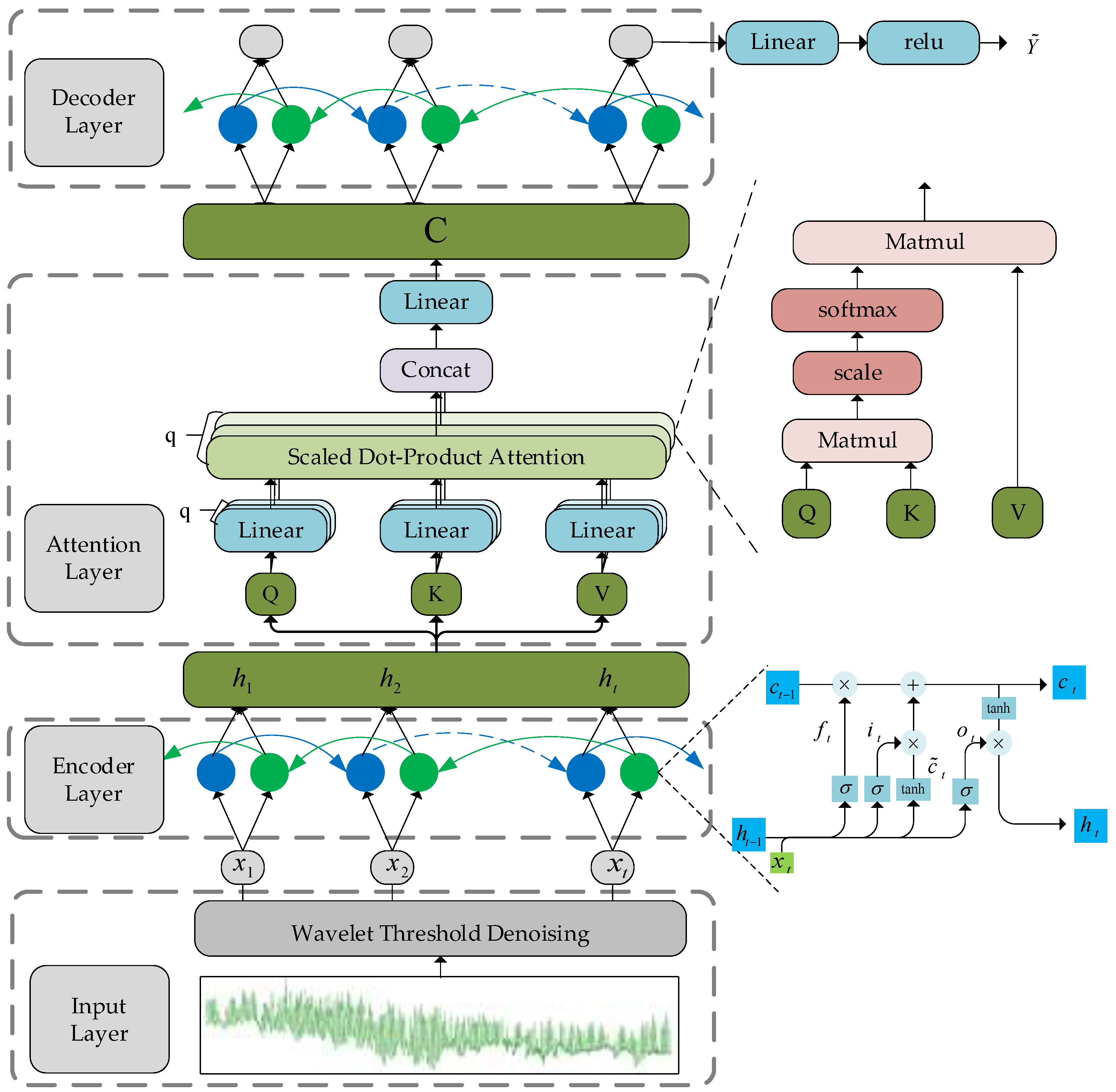
3.4. Bidirectional Self-Attentive Encoding-Decoding Framework

In this paper, we construct a self-attention prediction model based on the encoder–decoder framework. Although the encoder–decoder framework is classical, the limitations of fixed-length coding and information loss degrade the network performance as the input sequence increases. The attention mechanism overcomes the limitations of the encoder–decoder by performing attended feature selection on the encoder output. Multiheaded attention constructed by using a highly optimized matrix multiplication encoder is faster and more spatially efficient than additive attention and multiplicative attention. We use BiLSTM to build the encoder–decoder and fuse the self-attentive mechanism in the encoder–decoder. The model structure is shown in Figure 3.

As shown in Figure 3, the data is first subjected to sliding window and wavelet threshold denoising to obtain the filtered data $X={[x_1,x_2,\cdots ,x_t]}^T\in {ℝ}^t$ and the true value $Y={\left[y_{t+1},y_{t+2},\cdots ,y_{t+\tau }\right]}^T\in {ℝ}^{\tau }$. The encoder network consists of a multilayer BiLSTM network. After forward propagation of the input data $X$ through the encoder, the encoder output $H={\left[h_1,h_2,\cdots ,h_i,\cdots ,h_t\right]}^T\in {ℝ}^{t\times u}$ is obtained, where $u$ is the number of cells output by BiLSTM, $h_i=[{\overrightarrow{h}}_i;{\overleftarrow{h}}_i]$, and $[;]$ denotes the sum of two vectors.

In the multi-head attention layer, all of the queries, keys, and values come from the encoder output $H$. After encoder output $H$ has been nonlinearly mapped $k$ times, we obtain $k$ groups queries, keys, and values.

$$Q_i=\sigma \left(w_{q,i}H+b_{q,i}\right),i=1,2,\cdots ,k$$

(23)

$$K_i=\sigma \left(w_{k,i}H+b_{k,i}\right),i=1,2,\cdots ,k$$

(24)

$$V_i=\sigma \left(w_{v,i}H+b_{v,i}\right),i=1,2,\cdots ,k$$

(25)

where $w_{q,i}\in {ℝ}^{u\times d}$, $w_{k,i}\in {ℝ}^{u\times d}$, $w_{v,i}\in {ℝ}^{u\times d}$, $b_{q,i}\in {ℝ}^{t\times d}$, $b_{k,i}\in {ℝ}^{t\times d}$, $b_{v,i}\in {ℝ}^{t\times d}$ are the parameters to be learned, $d=\frac{u}{k}$, $Q_j\in {ℝ}^{t\times d}$, $K_j\in {ℝ}^{t\times d}$, and $V_j\in {ℝ}^{t\times d}$. The scaled dot product attention is computed for each of the $k$ groups Q, K, and V. The attention weight is a temporal attention weight, which is a vector of $t$ rows and $t$ columns.

$$hea{d}_i=soft\max \left(\frac{Q_i{K}_i^T}{\sqrt{d}}\right)V_i$$

(26)

All the results are concatenated and linearly transformed to obtain the output.

$$o=w_{o}concat(hea{d}_0,\dots ,hea{d}_h)+b_o$$

(27)

where $w_o\in {ℝ}^{u\times u}$, $b_o\in {ℝ}^{t\times u}$ are the parameters to be learned. Finally, we add the weighted encoder output to the original encoder output to obtain the encoding vector $C\in {ℝ}^{t\times u}$.

Similar to the encoder, the decoder is also composed of multiple layers of the BiLSTM network. In the decoder, the encoder vector $C$ is forward propagated and the decoder output $s$ is nonlinearly transformed to obtain the predicted value. The output layer transforms the output vector of the decoder linearly to a vector of variable dimension $\tau$, and then nonlinearly using the relu activation function to obtain the final predicted value.

$$\widehat{y}=relu\left(w_{y}s+b_y\right)$$

(28)

The training proceeds on the training set; after that, the evaluation is performed on the validation set for minimizing overfitting. When the training process and parameter selection are achieved, the final evaluation is performed on the unknown testing set for evaluating the performance. All models use the Adaptive Moment Estimation (Adam) optimization algorithm, which uses momentum and adaptive learning rates to speed up convergence, and it is computationally efficient and has a low memory footprint. The loss function for model training is the mean absolute error (MSE).

$$\mathrm{MSE}=\frac{{{\displaystyle {\sum }_{i=1}^n({\widehat{y}}_i-y_i)}}^2}{n}$$

(29)

where $n$ is the number of samples, $\widehat{y}$ is the predicted value, $y$ is the ground truth value. The MSE is derivable everywhere; the gradient values are dynamically changing and can converge quickly.

4. Results and Discussion

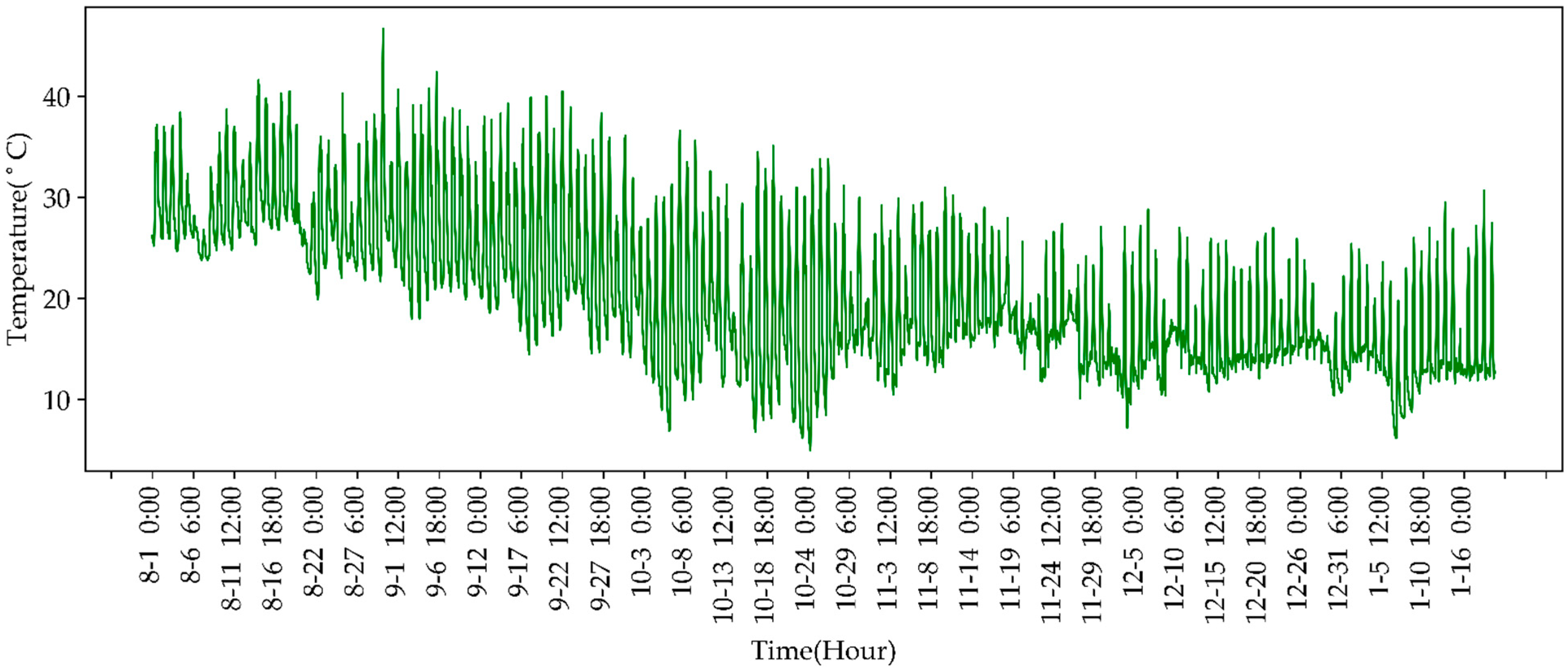
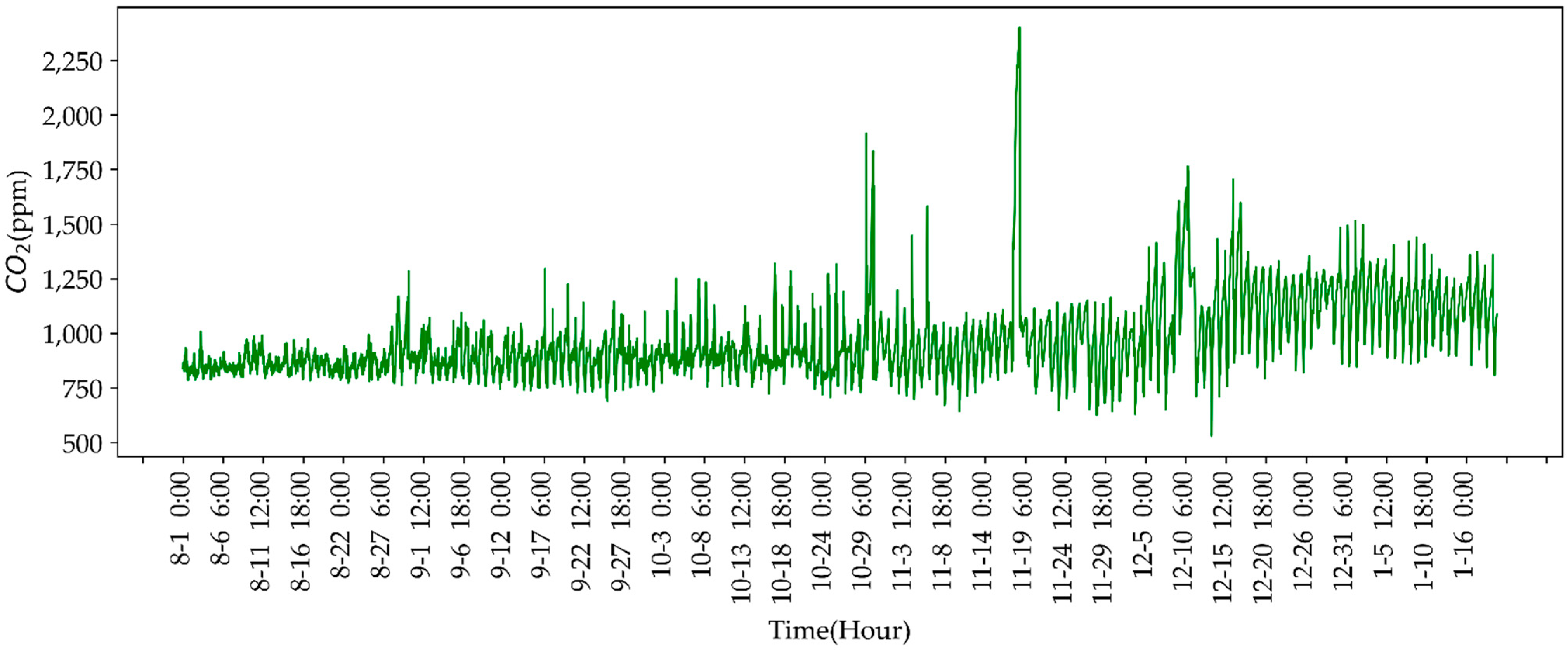
4.1. Experimental Datasets

All constructed datasets used in this experiment are real data derived from greenhouses in Weifang, Shandong, China, and collected by various environmental monitoring stations and IoT-based sensors, which are developed in-house by the Beijing Agricultural Intelligent Equipment Technology Research Centre. Each greenhouse is equipped with an intelligence management system to collect, analyze and process massive environmental information, including temperature, humidity, CO₂, light intensity and quanta, total radiation, net radiation, barometric pressure, wind direction, wind speed, and rainfall in the inside and outdoors of the whole greenhouse. The various parameters measuring the greenhouse are recorded by different devices at all times. Then, those data can be transferred to the cloud platform and stored in the management system’s database via the serial port at any time, as long as the computer is connected to the collector. Then, these data are automatically transmitted to the background cloud server through communication forms such as CAN/4G/WIFI at regular intervals, and are stored in the management system’s database via the serial port at any time, as long as the computer is connected to the collector. After data processing and intelligent model learning, the prediction results and determined recommendations are returned in a timely manner, which can more accurately reflect the dynamic situation of greenhouse management. The experimental greenhouse and inside scenes equipped with various IoT-based environmental monitoring sensors and stations are shown in Figure 4.

The dataset includes greenhouse air temperature, humidity, and CO₂ concentrations for a total of 172 days from 1 August 2020 to 19 January 2021, with a data sampling frequency of 30 min. The sensor acquisition data is relatively complete, with only a few missing values. For the missing parts of the data, mean interpolation is used. A total of 8256 sets of data were finally obtained. The waveforms of temperature, humidity, and CO₂ concentration are shown in Figure 5, Figure 6 and Figure 7.

The graphs show that the temperature, humidity, and CO₂ concentration data in the greenhouse are cyclical and fluctuating. The CO₂ concentration data are significantly higher after December than before December.

In the experimental section, we used the first 24 temperature data to predict the last 24 temperature data, i.e., the first 12 h to predict the last 12 h. Similarly, humidity and CO₂ concentration were also predicted by the first 24 data to the last 24 data. We used the first 158 days of data as training, and the last 28 days were divided equally into the validation and test sets. Due to the performance of the sensor and the measurement environment, the greenhouse data obtained from the sensor will inevitably be mixed with noise. The presence of noise can lead to overfitting of the model to the noise in the training set, resulting in a reduction in the prediction accuracy and robustness of the model. Therefore, the original dataset was denoised by wavelet threshold filtering. The local filter waveforms for temperature, humidity, and CO₂ concentration are shown in Figure 8, Figure 9 and Figure 10.

Here, the red waveform is the original data, and the green waveform is the wavelet threshold filtered data. As can be seen from the graphs, the curve is smoother after wavelet threshold filtering. The parameters for suitable wavelet threshold denoising were derived from several comparisons. In the temperature dataset, the parameters for using wavelet threshold denoising are wavelet basis: sym3, $N=3$, and scaling factor: 0.9, 0.5, and 0.4, respectively. In the humidity dataset, the parameters for using wavelet threshold denoising are wavelet basis: sym3, $N=3$, and scaling factor: 0.9, 0.6, and 0.6, respectively. In the CO₂ dataset, the parameters for using wavelet threshold denoising are wavelet basis: db3, $N=1$, and scaling factor: 0.3.

4.2. Evaluation Metrics

We evaluated the performance of the model using five evaluation metrics, including root mean square error (RMSE), mean absolute error (MAE), Pearson correlation coefficient (R), symmetric mean absolute percentage error (SMAPE), and complexity-invariant distance (CID). The formulae for calculating the first four indicators are shown below:

$$\mathrm{RMSE}=\sqrt{\frac{{{\displaystyle {\sum }_{i=1}^n({\widehat{y}}_i-y_i)}}^2}{n}}$$

(30)

$$\mathrm{MAE}=\frac{1}{n}{\displaystyle {\sum }_{i=1}^n\left|{\widehat{y}}_i-y_i\right|}$$

(31)

$$\mathrm{SMAPE}=\frac{1}{n}{\displaystyle {\sum }_{i=1}^n\frac{\left|{\widehat{y}}_i-y_i\right|}{(\left|{\widehat{y}}_i\right|+\left|y_i\right|)/2}}$$

(32)

$$\mathrm{R}=\frac{{\displaystyle {\sum }_{i=1}^n({\widehat{y}}_i-{\overline{\widehat{y}}}_i)(y_i-{\overline{y}}_i)}}{\sqrt{{\displaystyle {\sum }_{i=1}^n{({\widehat{y}}_i-{\overline{\widehat{y}}}_i)}^2{\displaystyle {\sum }_{i=1}^n{(y_i-{\overline{y}}_i)}^2}}}}$$

(33)

where $n$ is the number of samples, $\widehat{y}$ is the predicted value, $\overline{\widehat{y}}$ is the average of the prediction, $y$ is the ground truth value of the power load, and $\overline{y}$ is the average of the ground truth value.

In addition, we also used the complexity-invariant distance [48] metric to assess the information difference in complexity between the predicted and actual values. The complexity-invariant distance was proposed by Batista and originally used to measure the complexity difference between two time series by using information theory. For two time series, $\widehat{Y}=({\widehat{y}}_1,{\widehat{y}}_2,\cdots ,{\widehat{y}}_{\tau })$ and $y=(y_1,y_2,\cdots ,y_{\tau })$ of length, the statistic $CID(\widehat{Y},Y)$ can be calculated as follows:

$$CE(Y)=\sqrt{{{\displaystyle \sum _{t=1}^{\tau }(y_{t+1}-y_t)}}^2}$$

(34)

$$CF(\widehat{Y},Y)=\frac{\max \left\{CE(\widehat{Y}),CE(Y)\right\}}{\min \left\{CE(\widehat{Y}),CE(Y)\right\}}$$

(35)

$$ED(\widehat{Y},Y)=\sqrt{{{\displaystyle \sum _{t=1}^{\tau }({\widehat{y}}_t-y_t)}}^2}$$

(36)

$$CID(\widehat{Y},Y)=ED(\widehat{Y},Y)CF(\widehat{Y},Y)$$

(37)

Similar to the common evaluation metrics, a smaller CID means less difference between the two time series. It can effectively overcome the subjective similarities directly observed by the human eye.

4.3. Comparative Experiments

To validate the performance of our approach, we conducted some experiments to compare our proposed model with other advanced deep-learning models. In this paper, BP [29], LSTM [30], GRU, BiLSTM [49], encoder–decoder, and attention methods are used as comparison methods, where both encoder–decoder and attention were constructed using LSTM networks. All experimental models were written using the Torch deep-learning framework. Among them, the number of network layers of BP, LSTM, GRU, and BiLSTM is all four layers, and the number of network cells in each layer is 24. The encoder and decoder of encoder–decoder and attention are composed of two layers of the LSTM network. The encoder and decoder of the method in this paper are composed of two layers of the BiLSTM network. The number of attention heads in the attention model and the paper method is four. The batch size of all models is 16, the number of training iterations epoch is 100, the optimizer is Adam, and the learning rate is 0.001. All models were trained and tested on a cloud server platform with Windows 10 system, and codes are based on the open-source framework, Pytorch with Python API, and were run on a dual-core Intel Core i7-9750H@2.6 GHz processor with two NVIDIA RTX 2060 GPUs, which have 16 G memory.

To verify the stability of the models, each model was repeated 10 times independently in this paper, and the result indicators of each test set were statistically analyzed, and box-and-whisker plots were drawn. In the box-and-whisker plot, a line in the middle of the box, which is the median of the data, represents the average of the sample data. The upper and lower limits of the box, which are the upper and lower quartiles of the data, respectively, mean that the box contains 50% of the data, and the width of the box reflects, to some extent, the degree of fluctuation of the data. There is a line above and below the box, representing the maximum and minimum values. By relying on the box-and-whisker plot, we can roughly determine the dispersion of the data distribution. The average of the results of 10 model tests was used as the final evaluation of each model.

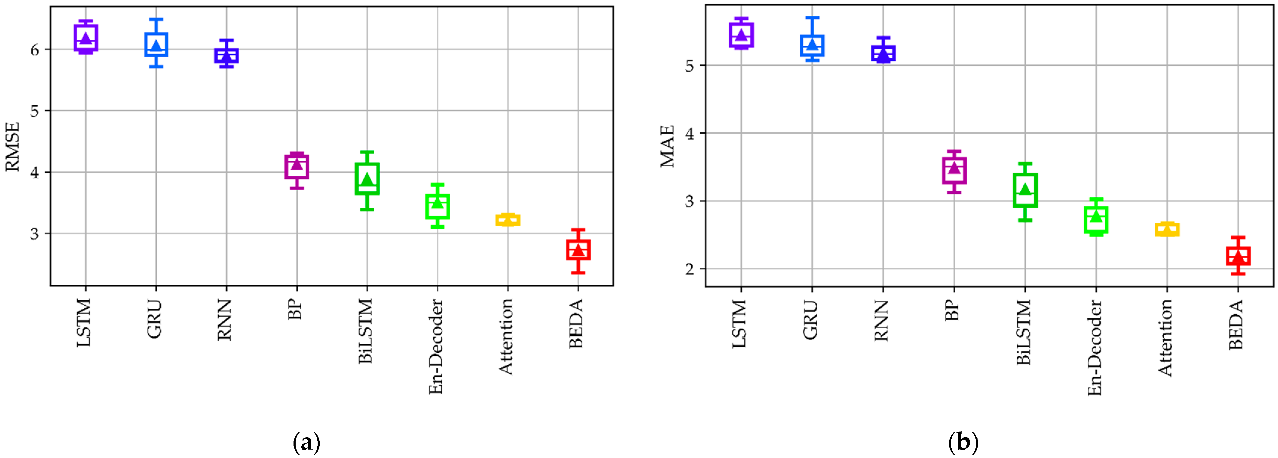
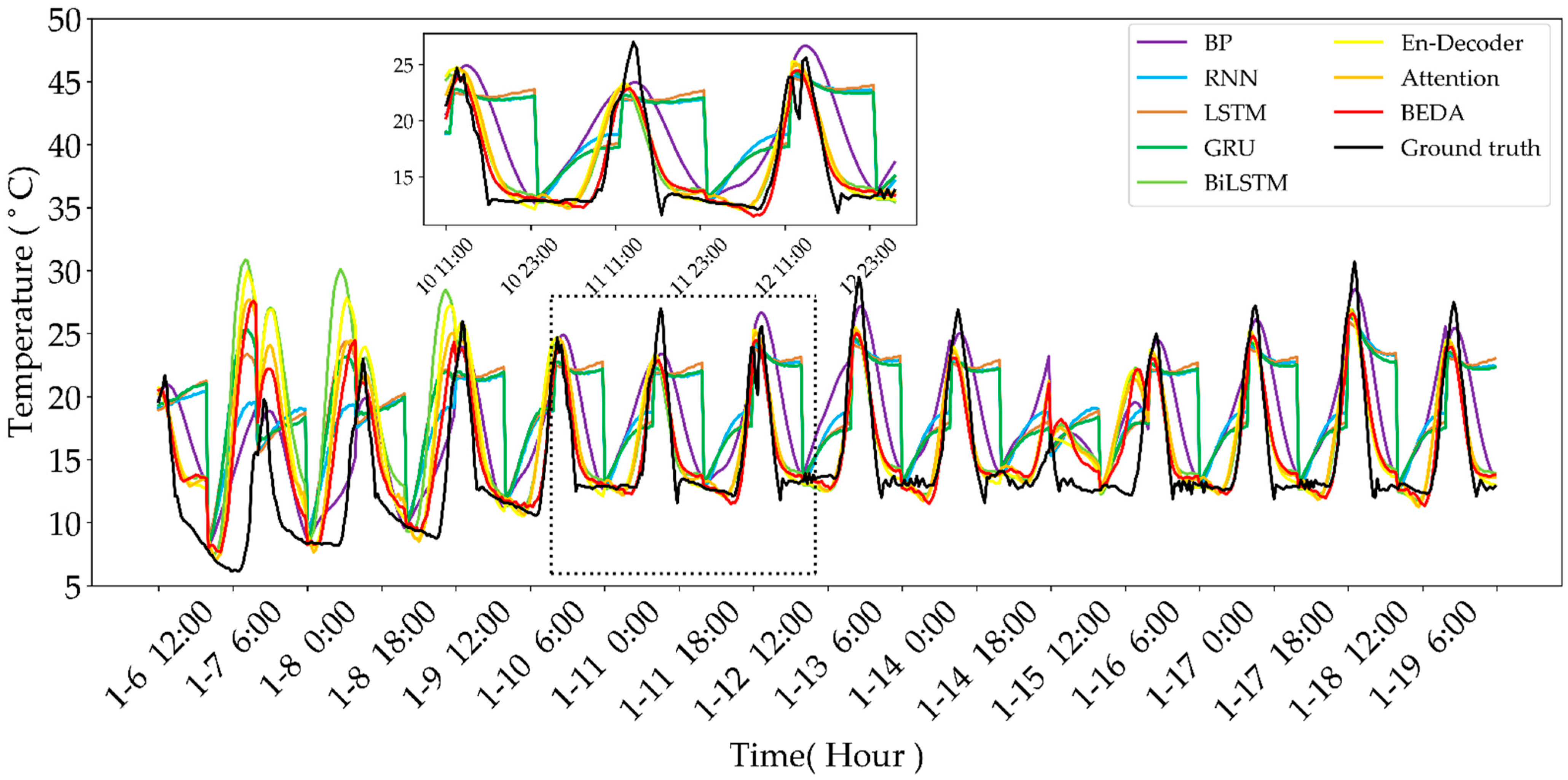
4.3.1. Temperature-Predicting Results

The RMSE box-and-whisker diagram and MAE box-and-whisker diagram for each model of the temperature dataset are shown in Figure 11. We can see, from Figure 11, that the LSTM, GRU, RNN, BP, and BiLSTM models have wider boxes and unstable models, and the attention model has the narrowest box and the most stable model. There is more stability and more accuracy with the encoder–decoder structure than without the encoder–decoder structure. The model is more stable and has higher prediction accuracy after incorporating the attention mechanism. Although the box of the paper’s method is wider than the attention model, its RMSE metric is smaller than that of attention model, highlighting the accuracy of the model and indicating that the use of bidirectional recurrent neural networks is effective for model performance improvement.

The temperature data in the greenhouse for each model index is shown in

Table 1. Model indicators for temperature in greenhouses.

Model	RMSE	MAE	SMAPE	R	CID
LSTM	6.179	5.451	0.333	0.377	254.5
GRU	6.054	5.31	0.326	0.399	249
RNN	5.888	5.186	0.322	0.481	228.2
BP	4.125	3.487	0.227	0.51	147.6
BiLSTM	3.887	3.169	0.193	0.517	145.2
Encoder–decoder	3.498	2.773	0.174	0.646	124.1
Attention	3.202	2.567	0.166	0.706	112.5
Proposed BEDA	2.726	2.183	0.144	0.749	97.38

. Figure 12 visualizes the evaluation indicators in Table 1. As can be seen from Table 1, the proposed method has the smallest RMSE, MAE, and SMAPE, the largest R, and the best curve fit. As can be seen from the table, using the encoder–decoder structure reduces RMSE, MAE, SMAPE, and CID by 43%, 49%, 47%, and 51%, respectively, compared to not using the encoder–decoder structure. Using BiLSTM reduces each model metric by 37%, 41%, 42%, and 43%, respectively, compared to LSTM. With the addition of the attention mechanism, the metrics of the encoder–decoder structure are reduced by 8%, 7%, 4%, and 9%, respectively. The metrics of encoder–decoder attention networks using BiLSTM decreased by 15%, 15%, 13%, and 13%, respectively, compared to those using LSTM.

Figure 13 shows the prediction waveforms of each model for the temperature data, which shows the temperature prediction curves from 6 January 2021 to 19 January 2021. In different parts of the prediction, the model in this paper does not perform the best, but in most of them, the prediction curve of the proposed method is the closest to the true curve. The local plot shows the prediction curve from January 10 to 12, in which the predicted values of the proposed method are closest to the true values.

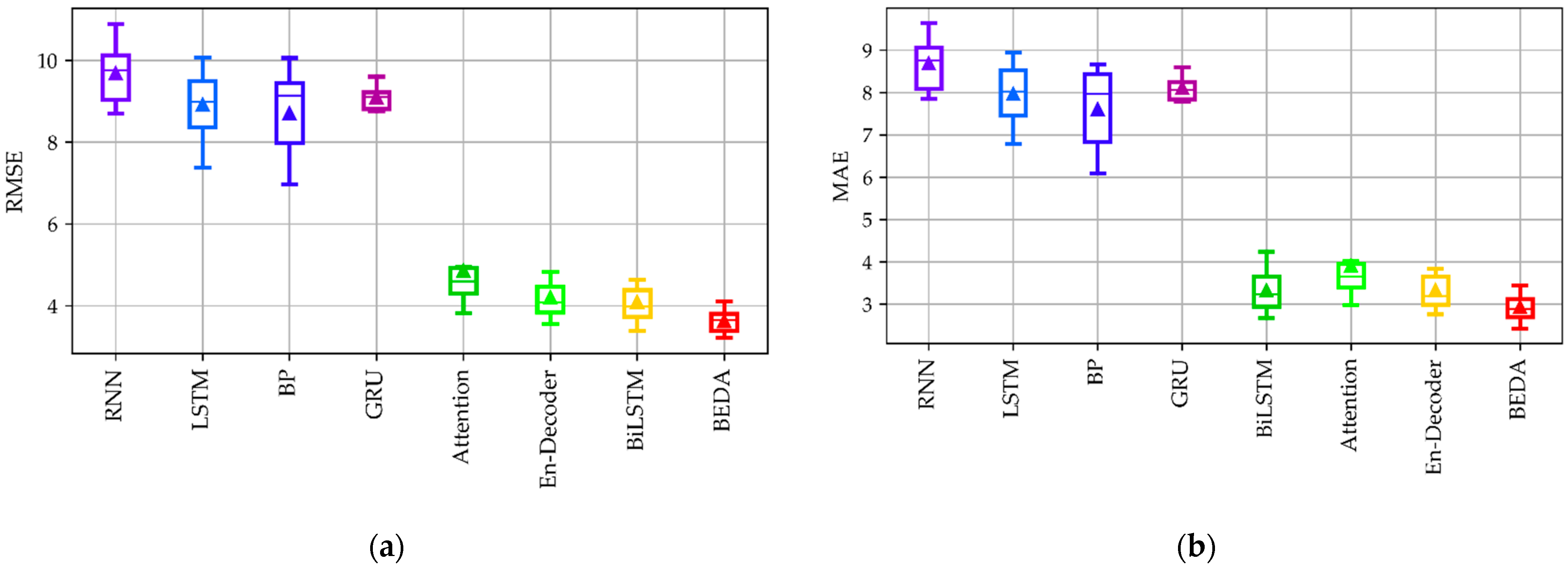
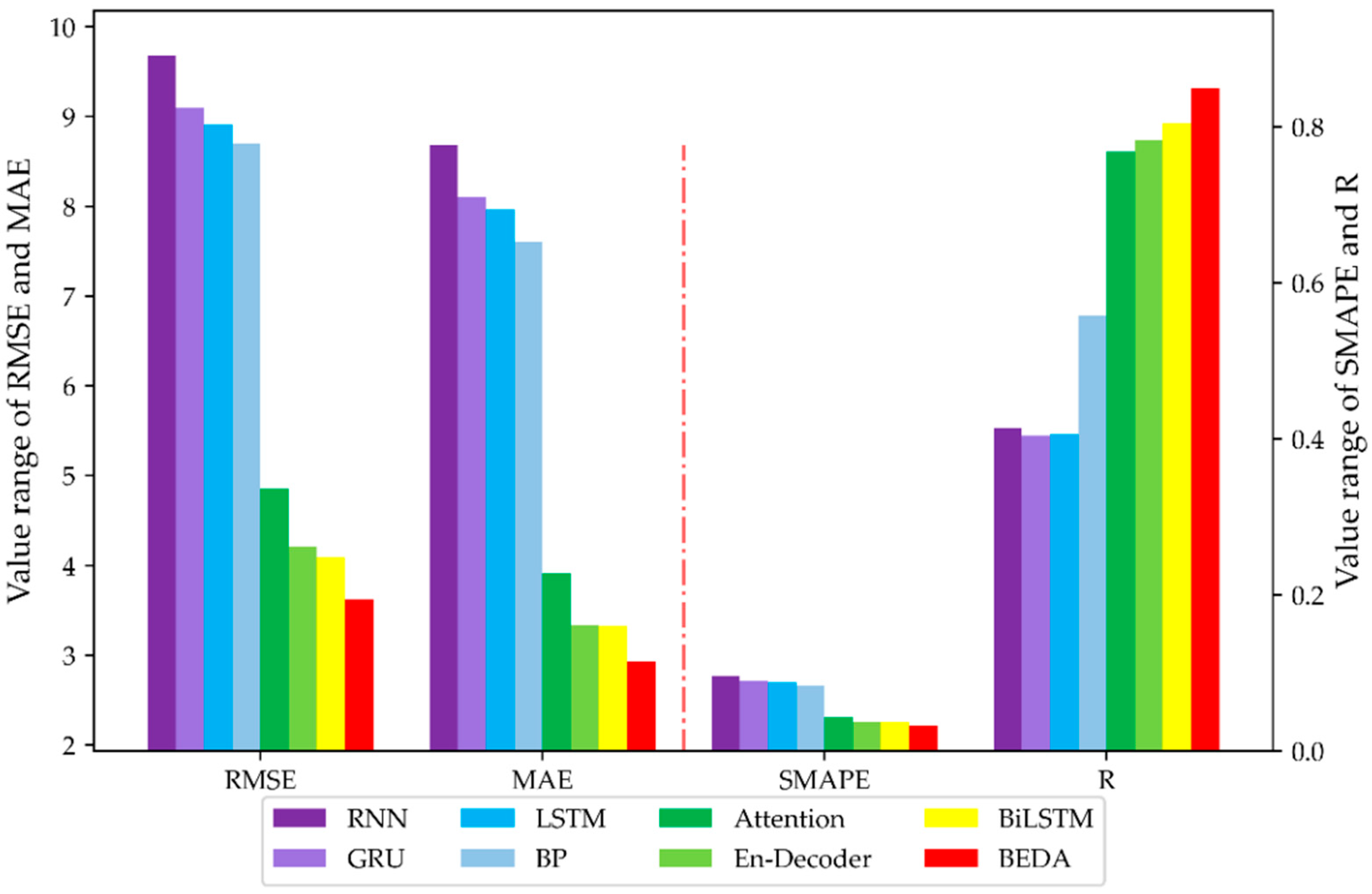
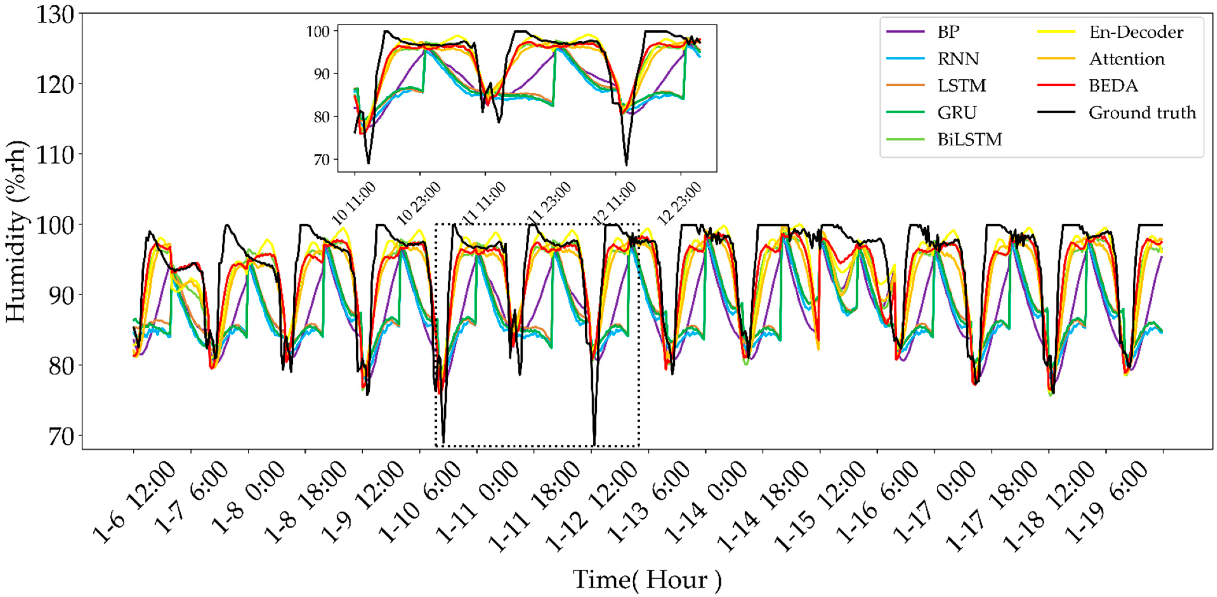
4.3.2. Humidity-Predicting Results

The RMSE box-and-whisker diagram and MAE box-and-whisker diagram for each model of the humidity dataset are shown in Figure 14. As can be seen from Figure 14, the RNN, LSTM, and BP models have wider boxes, unstable models, and low prediction accuracy. Although the GRU model has a narrower box, its RMSE and MAE are larger, and its prediction accuracy is low. The use of the encoder–decoder structure is more stable and accurate than the structure without the encoder–decoder. The inclusion of the attention mechanism resulted in a more stable model with higher prediction accuracy. BiLSTM showed good performance in the humidity dataset, while the encoder–decoder attention model was constructed with a smaller box using BiLSTM and the model had higher prediction accuracy.

The humidity data in the greenhouse for each model index is shown in

Table 2. Model indicators for humidity in greenhouses.

Model	RMSE	MAE	SMAPE	R	CID
RNN	9.680	8.683	0.0954	0.412	283.7
GRU	9.092	8.106	0.0888	0.403	257.7
LSTM	8.912	7.963	0.0872	0.406	259.5
BP	8.702	7.606	0.0834	0.557	355.1
Attention	4.851	3.90	0.0425	0.767	171.4
Encoder–decoder	4.201	3.335	0.0363	0.782	141.7
BiLSTM	4.093	3.325	0.0363	0.804	147.1
Proposed BEDA	3.621	2.934	0.0319	0.848	127.8

. Figure 15 visualizes the evaluation indicators in the Table 2. As can be seen from Table 2, the proposed method has the smallest RMSE, MAE, and SMAPE, the largest R, and the best curve fit. As can be seen from the table, using the encoder–decoder structure reduces RMSE, MAE, SMAPE, and CID by 52%, 58%, 58%, and 45%, respectively, compared to not using the encoder–decoder structure. Using BiLSTM reduces each model metric by 54%, 58%, 58%, and 43%, respectively, compared to LSTM. The metrics of encoder–decoder attention networks using BiLSTM decreased by 13%, 12%, 12%, and 9%, respectively, compared to those using LSTM.

Figure 16 shows the prediction waveforms of each model for the humidity data, which shows the humidity prediction curves from 6 January 2021 to 19 January 2021. In different parts of the prediction, the model in this paper does not perform the best, but in most of them, the prediction curve of the proposed method is the closest to the true curve. The local plot shows the prediction curve from January 10 to 12, in which the predicted values of the proposed method are closest to the true values.

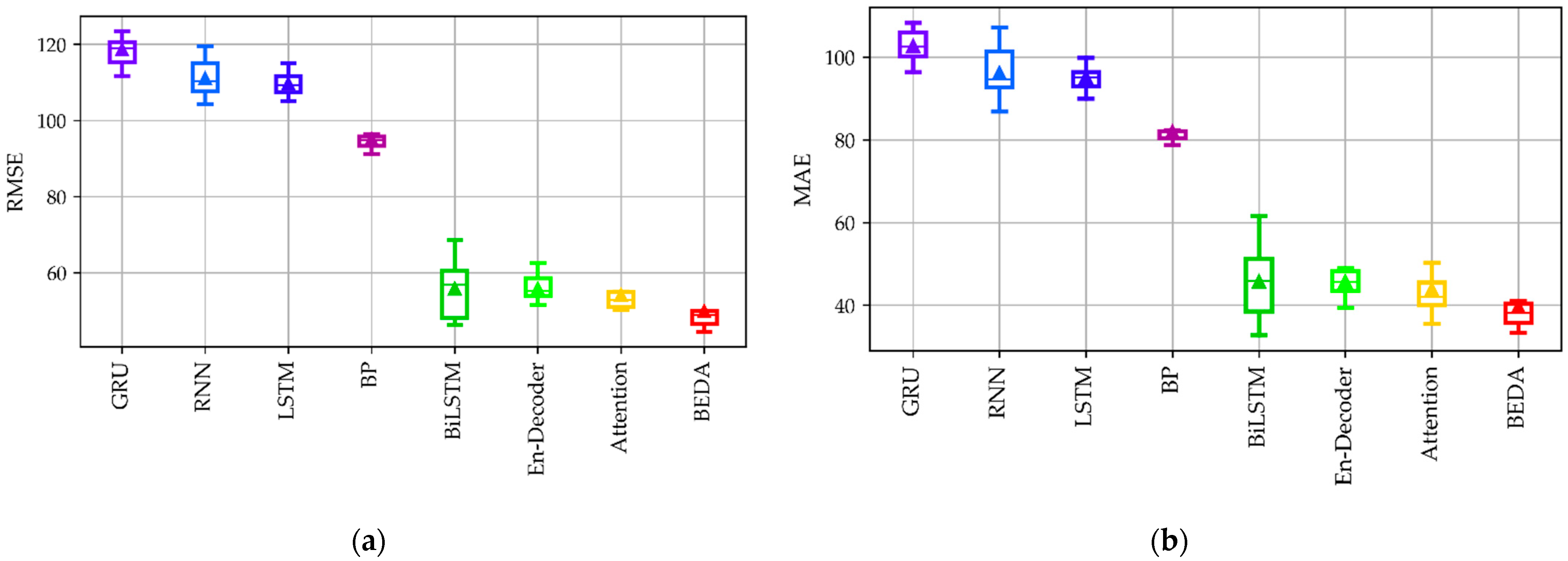
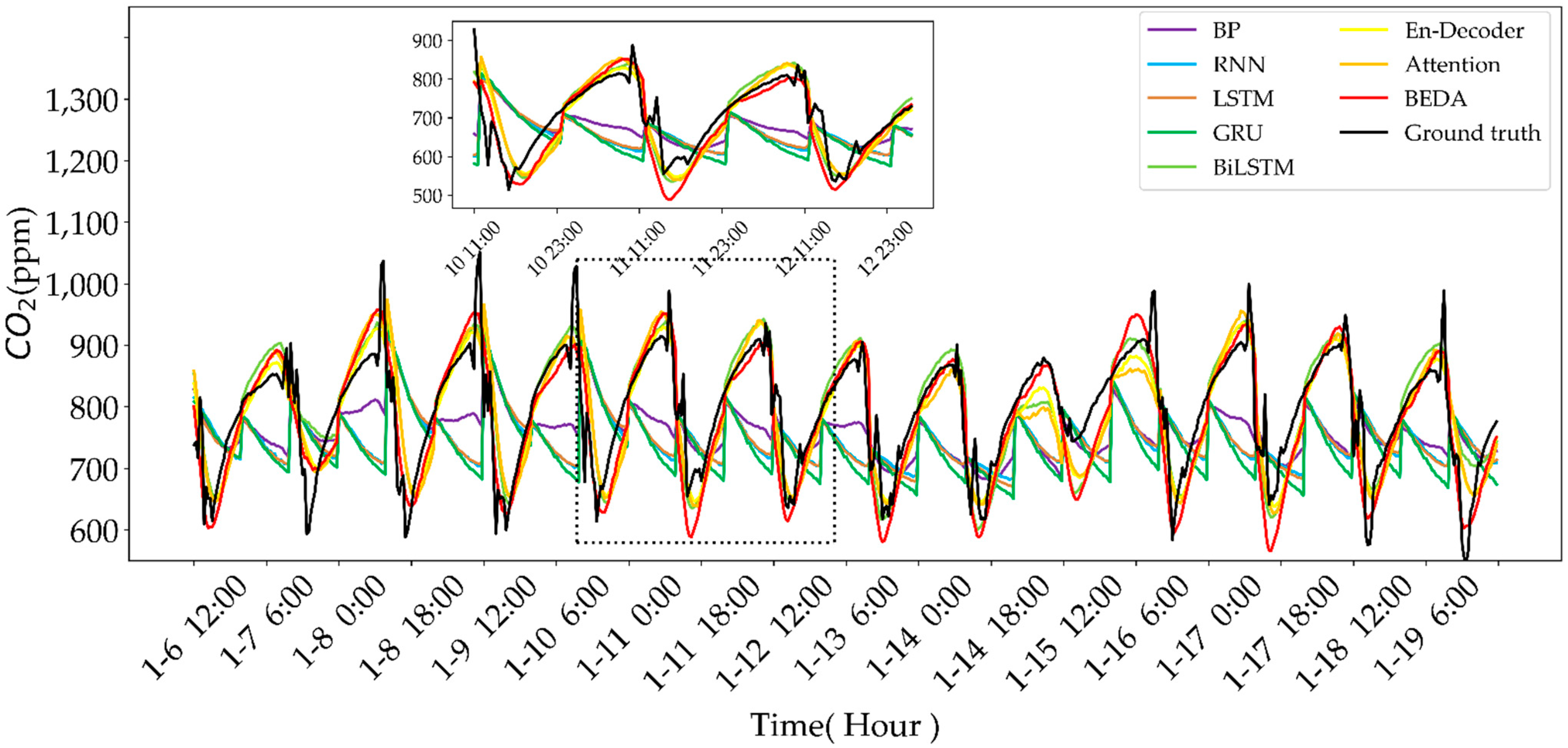
4.3.3. CO₂ Concentration-Predicting Results

The RMSE box-and-whisker diagram and MAE box-and-whisker diagram for each model of the CO₂ dataset are shown in Figure 17. As can be seen from Figure 17, the GRU, RNN, LSTM, and BiLSTM models have wider boxes, unstable models, and low prediction accuracy. Although the BP model has a narrower box, its RMSE and MAE are larger, and its prediction accuracy is low. The use of encoder–decoder structures is more stable and accurate than structures without encoder–decoders. The introduction of the attention mechanism means the model is more stable and has higher prediction accuracy. The encoder–decoder attention model constructed using BiLSTM has high prediction accuracy and stability.

The CO₂ data in the greenhouse for each model index is shown in

Table 3. Model indicators for CO₂ in greenhouses.

Model	RMSE	MAE	SMAPE	R	CID
GRU	118.610	102.699	0.1526	0.1723	4046.4
RNN	111.068	96.196	0.1420	0.1601	4773.2
LSTM	109.683	95.131	0.1403	0.1369	5135.1
BP	95.083	81.975	0.1201	0.1626	5432.7
BiLSTM	55.821	45.712	0.0683	0.8087	2576.6
Encoder–decoder	55.782	45.796	0.0683	0.8125	2652.1
Attention	54.110	43.883	0.0664	0.8405	2541.8
Proposed BEDA	49.817	39.640	0.0590	0.8711	2221.4

. Figure 18 visualizes the evaluation indicators in Table 3. As can be seen from Table 3, the proposed method has the smallest RMSE, MAE, and SMAPE, the largest R, and the best curve fit. As can be seen from the table, using the encoder–decoder structure reduces RMSE, MAE, SMAPE, and CID by 49%, 51%, 51%, and 48%, respectively, compared to not using the encoder–decoder structure. Using BiLSTM reduces each model metric by 49%, 51%, 51%, and 49%, respectively, compared to LSTM. With the addition of the attention mechanism, the metrics of the encoder–decoder structure are reduced by 3%, 4%, 2%, and 4%, respectively. The metrics of encoder–decoder attention networks using BiLSTM decreased by 8%, 9%, 11%, and 12%, respectively, compared to those using LSTM.

Figure 19 shows the prediction waveforms of each model for the CO₂ data, which shows the CO₂ prediction curves from 6 January 2021 to 19 January 2021. In different parts of the prediction, the model in this paper does not perform the best, but in most of them, the prediction curve of the proposed method is the closest to the true curve. The local plot shows the prediction curve from January 10 to 12, in which the predicted values of the proposed method are closest to the true values.

Figure 20 shows a scatter plot of the test results for the three dataset test sets of temperature humidity and CO₂, with the horizontal axis representing the true values and the vertical axis representing the predicted values. The blue dots are the distribution of all predicted values, the black dots are the distribution of the true values, the red line is the regression fit line for the predicted values, and the black line represents the true values. The slope of the black line is 1. The slopes of the regression lines for the predicted results of the test sets for temperature, humidity, and CO₂ were calculated to be 0.678, 0.754, and 1.039, respectively.

It was shown, with the greenhouse temperature, humidity, and CO₂ datasets, that the encoder–decoder model performs better than other commonly used models for time series data with high randomness and volatility. The encoder–decoder model can better extract data features and dig deeper into the feature patterns within the data. The incorporation of attention can even effectively improve the stability and prediction accuracy of the model. BiLSTM has better performance than LSTM by extracting learned column data features in both forward and backward directions. The bidirectional self-attentive encoder–decoder model showed good stability and prediction accuracy on all three datasets.

5. Conclusions

Within the trend of a progressive adoption of IoT and artificial intelligence technologies in agriculture, we considered the specific problem of developing temporal predictors for environmental factors in smart greenhouses embedding IoT sensors. The model is based on a bidirectional self-attentive encoder–decoder framework (BEDA) for forecasting multiple environmental factors with strong nonlinearity and noise. In the proposed method, the integrity and accuracy of data are effectively improved after wavelet threshold denoising and data pretreatment operation in the first stage. Then, the bidirectional long short-term memory (LSTM) is selected as the fundamental unit to extract time-serial features. Ultimately, the multi-head self-attention mechanism is incorporated into the encoder–decoder framework to construct the prediction model. The prediction results of temperature, humidity, and CO₂ using the constructed BEDA method show that the proposed predictor can achieve better accuracy, robustness, and generalization performance than the comparative prediction models. Specifically, for the root mean square error, the prediction results of the proposed method can fall to 2.726 for temperature, 3.621 for humidity, and 49.817 for CO₂ concentration, respectively, with an R of 0.749, 0.848, and 0.8711 for three parameters. Experimental results show that the proposed method is much more suitable for smart greenhouse management and application. In further work, the model structure will be optimized to improve the prediction performance, and the coupling of greenhouse data will be investigated to expand the application scope of the proposed model in smart agriculture. The proposed methods in this paper can combine other identification schemes [50,51,52,53,54,55] for studying new modeling and prediction of dynamic time series and dynamical systems with colored noises [56,57,58,59,60], and can be applied to other fields [61,62,63,64,65,66] such as signal modeling, tracking, and control systems.

References

1. Kksal, O.; Tekinerdogan, B. Architecture design approach for IoT-based farm management information systems. Precis. Agric. 2019, 20, 926–958. [Google Scholar] [CrossRef] [Green Version]
2. Eli-Chukwu, N.; Ogwugwam, E.C. Applications of artificial intelligence in agriculture: A review. Eng. Technol. Appl. Sci. Res. 2019, 9, 4377–4383. [Google Scholar] [CrossRef]
3. Jirapond, M.; Nathaphon, B.; Siriwan, K.; Narongsak, L.; Apirat, W.; Pichetwut, N. IoT and agriculture data analysis for smart farm. Comput. Electron. Agric. 2019, 156, 467–474. [Google Scholar]
4. Zhang, C.; Liu, Z. Application of big data technology in agricultural internet of things. Int. J. Distrib. Sens. Netw. 2019, 15, 155014771988161. [Google Scholar] [CrossRef]
5. Dananjayan, S. A survey on the 5G network and its impact on agriculture: Challenges and opportunities. Comput. Electron. Agric. 2020, 180, 105895. [Google Scholar]
6. Mta, C.; Aehb, C. Integrating blockchain and the internet of things in precision agriculture: Analysis, opportunities, and challenges. Comput. Electron. Agric. 2020, 178, 105476. [Google Scholar]
7. Jin, X.B.; Yang, N.X.; Wang, X.Y.; Bai, Y.T.; Kong, J.L. Hybrid deep learning predictor for smart agriculture sensing based on empirical mode decomposition and gated recurrent unit group model. Sensors 2020, 20, 1334. [Google Scholar] [CrossRef] [Green Version]
8. Xu, L.; Xiong, W.L.; Alsaedi, A.; Hayat, T. Hierarchical parameter estimation for the frequency response based on the dynamical window data. Int. J. Control Autom. Syst. 2018, 16, 1756–1764. [Google Scholar] [CrossRef]
9. Sun, Q. Ecological agriculture development and spatial and temporal characteristics of carbon emissions of land use. Appl. Ecol. Environ. Res. 2019, 17, 17. [Google Scholar] [CrossRef]
10. Kolasa-Więcek, A. Use of Artificial neural networks in predicting direct nitrous oxide emissions from agricultural soils. Ecol. Chem. Eng. 2013, 20, 419–428. [Google Scholar] [CrossRef]
11. Ayele, T.W.; Mehta, R. Real time temperature prediction using IoT. In Proceedings of the 2nd IEEE International Conference on Inventive Communication and Computational Technologies, Coimbatore, India, 20–21 April 2018; pp. 1114–1117. [Google Scholar]
12. Ding, F.; Zhang, X.; Xu, L. The innovation algorithms for multivariable state-space models. Int. J. Adapt. Control Signal Process. 2019, 33, 1601–1608. [Google Scholar] [CrossRef]
13. Ding, F.; Ma, H.; Pan, J.; Yang, E. Hierarchical gradient- and least squares-based iterative algorithms for input nonlinear output-error systems using the key term separation. J. Frankl. Inst. 2021, 358, 5113–5135. [Google Scholar] [CrossRef]
14. Ding, F.; Chen, H.; Xu, L.; Dai, J.; Li, Q.; Hayat, T. A hierarchical least squares identification algorithm for Hammerstein nonlinear systems using the key term separation. J. Frankl. Inst. 2018, 355, 3737–3752. [Google Scholar] [CrossRef]
15. Xu, L.; Song, G. A recursive parameter estimation algorithm for modeling signals with multi-frequencies. Circuits Syst. Signal Process. 2020, 39, 4198–4224. [Google Scholar] [CrossRef]
16. Li, M.; Liu, X. Maximum likelihood hierarchical least squares-based iterative identification for dual-rate stochastic systems. Int. J. Adapt. Control Signal Process. 2021, 35, 240–261. [Google Scholar] [CrossRef]
17. Li, M.; Liu, X. Iterative parameter estimation methods for dual-rate sampled-data bilinear systems by means of the data filtering technique. IET Control Theory Appl. 2021, 15, 1230–1245. [Google Scholar] [CrossRef]
18. Ding, F. Coupled-least-squares identification for multivariable systems. IET Control Theory Appl. 2013, 7, 68–79. [Google Scholar] [CrossRef]
19. Ding, F.; Xu, L.; Meng, D.D. Gradient estimation algorithms for the parameter identification of bilinear systems using the auxiliary model. J. Comput. Appl. Math. 2020, 369, 112575. [Google Scholar] [CrossRef]
20. Pan, J.; Jiang, X.; Wan, X.; Ding, W. A filtering based multi-innovation extended stochastic gradient algorithm for multivariable control systems. Int. J. Control Autom. Syst. 2017, 15, 1189–1197. [Google Scholar] [CrossRef]
21. Pan, J.; Ma, H.; Zhang, X.; Liu, Q.Y. Recursive coupled projection algorithms for multivariable output-error-like systems with coloured noises. IET Signal Process. 2020, 14, 455–466. [Google Scholar] [CrossRef]
22. Ding, F.; Liu, X.; Chu, J. Gradient-based and least-squares-based iterative algorithms for Hammerstein systems using the hierarchical identification principle. IET Control Theory Appl. 2013, 7, 176–184. [Google Scholar] [CrossRef]
23. Ding, F. Decomposition based fast least squares algorithm for output error systems. Signal Process. 2013, 93, 1235–1242. [Google Scholar] [CrossRef]
24. Ding, F. Hierarchical multi-innovation stochastic gradient algorithm for Hammerstein nonlinear system modeling. Appl. Math. Model. 2013, 37, 1694–1704. [Google Scholar] [CrossRef]
25. Li, M.; Liu, X. Maximum likelihood least squares based iterative estimation for a class of bilinear systems using the data filtering technique. Int. J. Control Autom. Syst. 2020, 18, 1581–1592. [Google Scholar] [CrossRef]
26. Li, M.; Liu, X. The least squares based iterative algorithms for parameter estimation of a bilinear system with autoregressive noise using the data filtering technique. Signal Process. 2018, 147, 23–34. [Google Scholar] [CrossRef]
27. Ding, F. Two-stage least squares based iterative estimation algorithm for CARARMA system modeling. Appl. Math. Model. 2013, 37, 4798–4808. [Google Scholar] [CrossRef]
28. Ding, F.; Xu, L.; Zhu, Q. Performance analysis of the generalised projection identification for time-varying systems. IET Control Theory Appl. 2016, 10, 2506–2514. [Google Scholar] [CrossRef] [Green Version]
29. Beverena, P.J.M.; Bontsemab, J.; Stratenc, G.; Hentena, E.J. Minimal Heating and Cooling in a Modern Rose Greenhouse. Appl. Energy 2015, 137, 97–109. [Google Scholar] [CrossRef]
30. Berroug, F.; Lakhal, E.K.; Omari, M.E.; Faraji, M.; Qarnia, H.E. Thermal performance of a greenhouse with a phase change material north wall. Energy Build. 2012, 43, 3027–3035. [Google Scholar] [CrossRef]
31. Rasheed, A.; Kwak, C.S.; Na, W.H.; Lee, J.W.; Kim, H.T.; HyunWoo, L. Development of a building energy simulation model for control of multi-span greenhouse microclimate. Agronomy 2020, 10, 1236. [Google Scholar] [CrossRef]
32. Yu, H.; Chen, Y.; Hassan, S.G.; Li, D. Prediction of the temperature in a Chinese solar greenhouse based on LSSVM optimized by improved PSO. Comput. Electron. Agric. 2016, 122, 94–102. [Google Scholar] [CrossRef]
33. Linker, R.; Seginer, I.; Gutman, P.O. Optimal CO2 control in a greenhouse modeled with neural networks. Comput. Electron. Agric. 1998, 19, 289–310. [Google Scholar] [CrossRef]
34. Ferreira, P.M.; FariaE, A.; RuanoA, E. Neural network models in greenhouse air temperature prediction. Neurocomputing 2002, 43, 51–75. [Google Scholar] [CrossRef] [Green Version]
35. Fourati, F.; Chtourou, M. A greenhouse control with feed-forward and recurrent neural networks. Simul. Model. Pract. Theory 2007, 15, 1016–1028. [Google Scholar] [CrossRef]
36. Zheng, Y.Y.; Kong, J.L.; Jin, X.B.; Wang, X.Y.; Zuo, M. CropDeep: The crop vision dataset for deep-learning-based classification and detection in precision agriculture. Sensors 2019, 19, 1058. [Google Scholar] [CrossRef] [Green Version]
37. Zheng, Y.Y.; Kong, J.L.; Jin, X.B.; Wang, X.Y.; Su, T.L.; Wang, J.L. Probability fusion decision framework of multiple deep neural networks for fine-grained visual classification. IEEE Access 2019, 7, 122740–122757. [Google Scholar] [CrossRef]
38. Zhen, T.; Kong, J.L.; Yan, L. Hybrid deep-learning framework based on gaussian fusion of multiple spatiotemporal networks for walking gait phase recognition. Complexity 2020, 2020, 1–17. [Google Scholar] [CrossRef]
39. Shi, Z.G.; Bai, Y.T.; Jin, X.B.; Wang, X.Y.; Su, T.L.; Kong, J.L. Parallel deep prediction with covariance intersection fusion on non-stationary time series. Knowl. Based Syst. 2021, 211, 106523. [Google Scholar] [CrossRef]
40. Jin, X.B.; Yu, X.H.; Su, T.L.; Yang, D.N.; Wang, L. Distributed deep fusion predictor for a multi-sensor system based on causality entropy. Entropy 2021, 23, 219. [Google Scholar] [CrossRef]
41. Perez, I.G.; Godoy, A.J.C. Neural networks-based models for greenhouse climate control. In Proceedings of the XXXIX Jornadas de Automática, Badajoz, Spain, 5–7 September 2018; pp. 875–879. [Google Scholar]
42. Song, Y.E.; Moon, A.; An, S.Y.; Jung, H. Prediction of smart greenhouse temperature-humidity based on multi-dimensional LSTMs. J. Korean Soc. Precis. Eng. 2019, 36, 239–246. [Google Scholar] [CrossRef]
43. Jin, X.B.; Zheng, W.Z.; Kong, J.L.; Wang, X.Y.; Bai, Y.T.; Su, T.L.; Lin, S. Deep-learning forecasting method for electric power load via attention-based encoder-decoder with bayesian optimization. Energies 2021, 14, 1596. [Google Scholar] [CrossRef]
44. Shi, P.F.; Fang, X.L.; Ni, J.J.; Zhu, J.X. An Improved attention-based integrated deep neural network for PM2.5 concentration prediction. Appl. Sci. 2021, 11, 4001. [Google Scholar] [CrossRef]
45. Luong, M.; Pham, H.; Manning, C.D. Effective approaches to attention-based neural machine translation. arXiv 2015, arXiv:1508.04025. [Google Scholar]
46. Zhao, Z.Y.; Wang, X.Y.; Yao, P.; Bai, Y.T. A health performance evaluation method of multirotors under wind turbulence. Nonlinear Dyn. 2020, 102, 1–15. [Google Scholar] [CrossRef]
47. Jin, X.-B.; Zhang, J.-H.; Su, T.-L.; Bai, Y.-T.; Kong, J.-L.; Wang, X.-Y. Modeling and Analysis of Data-Driven Systems through Computational Neuroscience Wavelet-Deep Optimized Model for Nonlinear Multicomponent Data Forecasting. Comput. Intell. Neurosci. 2021, 2021, 1–13. [Google Scholar] [CrossRef]
48. Batista, G.; Keogh, E.J.; Tataw, O.M.; De Souza, V.M. CID: An efficient complexity-invariant distance for time series. Data Min. Knowl. Discov. 2014, 28, 634–669. [Google Scholar] [CrossRef]
49. Moon, T.; Son, J.E. Knowledge transfer for adapting pre-trained deep neural models to predict different greenhouse environments based on a low quantity of data. Comput. Electron. Agric. 2021, 185, 106136. [Google Scholar] [CrossRef]
50. Ding, F. State filtering and parameter estimation for state space systems with scarce measurements. Signal Process. 2014, 104, 369–380. [Google Scholar] [CrossRef]
51. Ding, F. Combined state and least squares parameter estimation algorithms for dynamic systems. Appl. Math. Model. 2014, 38, 403–412. [Google Scholar] [CrossRef]
52. Liu, Y.; Shi, Y. An efficient hierarchical identification method for general dual-rate sampled-data systems. Automatica 2014, 50, 962–970. [Google Scholar] [CrossRef]
53. Zhang, X.; Liu, Q.Y. Recursive identification of bilinear time-delay systems through the redundant rule. J. Frankl. Inst. 2020, 257, 726–747. [Google Scholar] [CrossRef]
54. Zhang, X. Recursive parameter estimation and its convergence for bilinear systems. IET Control Theory Appl. 2020, 14, 677–688. [Google Scholar] [CrossRef]
55. Ding, F.; Zhan, X.; Alsaedi, A.; Hayat, T. Hierarchical extended least squares estimation approaches for a multi-input multi-output stochastic system with colored noise from observation data. J. Frankl. Inst. 2020, 357, 11094–11110. [Google Scholar] [CrossRef]
56. Xu, L.; Sheng, J. Hierarchical multi-innovation generalised extended stochastic gradient methods for multivariable equation-error autoregressive moving average systems. IET Control Theory Appl. 2020, 14, 1276–1286. [Google Scholar] [CrossRef]
57. Xu, L.; Sheng, J. Separable multi-innovation stochastic gradient estimation algorithm for the nonlinear dynamic responses of systems. Int. J. Adapt. Control Signal Process. 2020, 34, 937–954. [Google Scholar] [CrossRef]
58. Zhang, X.; Hayat, T. Recursive parameter identification of the dynamical models for bilinear state space systems. Nonlinear Dyn. 2017, 89, 2415–2429. [Google Scholar] [CrossRef]
59. Zhang, X.; Hayat, T. Combined state and parameter estimation for a bilinear state space system with moving average noise. J. Frankl. Inst. 2018, 355, 3079–3103. [Google Scholar] [CrossRef]
60. Zhou, Y. Modeling nonlinear processes using the radial basis function-based state-dependent autoregressive models. IEEE Signal Process. Lett. 2020, 27, 1600–1604. [Google Scholar] [CrossRef]
61. Xu, L.; Yang, E. Separable recursive gradient algorithm for dynamical systems based on the impulse response signals. Int. J. Control Autom. Syst. 2020, 18, 3167–3177. [Google Scholar] [CrossRef]
62. Ding, F.; Lv, L.; Pan, J.; Wan, X.; Jin, X. Two-stage gradient-based iterative estimation methods for controlled autoregressive systems using the measurement data. Int. J. Control Autom. Syst. 2020, 18, 886–896. [Google Scholar] [CrossRef]
63. Pan, J.; Li, W.; Zhang, H. Control algorithms of magnetic suspension systems based on the improved double exponential reaching law of sliding mode control. Int. J. Control Autom. Syst. 2018, 16, 2878–2887. [Google Scholar] [CrossRef]
64. Xu, L.; Chen, F.; Hayat, T. Hierarchical recursive signal modeling for multi-frequency signals based on discrete measured data. Int. J. Adapt. Control Signal Process. 2021, 35, 676–693. [Google Scholar] [CrossRef]
65. Kong, J.L.; Wang, Z.N.; Jin, X.B.; Wang, X.Y.; Su, T.L.; Wang, J.L. Semi-supervised segmentation framework based on spot-divergence supervoxelization of multi-sensor fusion data for autonomous forest machine applications. Sensors 2018, 18, 3061. [Google Scholar] [CrossRef] [Green Version]
66. Kong, J.L.; Wang, H.X.; Wang, X.Y.; Jin, X.B.; Fang, X.; Lin, S. Multi-stream hybrid architecture based on cross-level fusion strategy for fine-grained crop species recognition in precision agriculture. Comput. Electron. Agric. 2021, 182, 106134. [Google Scholar] [CrossRef]
Figure 1. Window sliding to generate model training data.
Agriculture 11 00802 g001
Figure 2. Bidirectional long short-term memory model structure.
Agriculture 11 00802 g002
Figure 3. Bidirectional self-attentive encoder–decoder model structure.
Agriculture 11 00802 g003
Figure 4. Intelligent greenhouse systems.
Agriculture 11 00802 g004
Figure 5. Waveforms of original data from the temperature dataset.
Agriculture 11 00802 g005
Figure 6. Waveforms of original data from the humidity dataset.
Agriculture 11 00802 g006
Figure 7. Waveforms of original data from the CO2 dataset.
Agriculture 11 00802 g007
Figure 8. Temperature data after wavelet threshold filtering.
Agriculture 11 00802 g008
Figure 9. Humidity data after wavelet threshold filtering.
Agriculture 11 00802 g009
Figure 10. CO2 data after wavelet threshold filtering.
Agriculture 11 00802 g010
Figure 11. Temperature dataset indicator box plots for each model. (a) RMSE box and whiskers for each model of the temperature dataset; (b) MAE box and whiskers for each model of the temperature dataset.
Agriculture 11 00802 g011
Figure 12. Histogram of each model test indicator for indoor temperature data.
Agriculture 11 00802 g012
Figure 13. Waveforms of test results for each model of indoor temperature data.
Agriculture 11 00802 g013
Figure 14. Humidity dataset indicator box plots for each model. (a) RMSE box and whiskers for each model of the humidity dataset; (b) MAE box and whiskers for each model of the humidity dataset.
Agriculture 11 00802 g014
Figure 15. Histogram of each model test indicator for indoor humidity data.
Agriculture 11 00802 g015
Figure 16. Waveforms of test results for each model of indoor humidity data.
Agriculture 11 00802 g016
Figure 17. CO2 dataset indicator box plots for each model. (a) RMSE box and whiskers for each model of the CO2 dataset; (b) MAE box and whiskers for each model of the CO2 dataset.
Agriculture 11 00802 g017
Figure 18. Histogram of each model test indicator for indoor CO2 data.
Agriculture 11 00802 g018
Figure 19. Waveforms of test results for each model of indoor CO2 data.
Agriculture 11 00802 g019
Figure 20. Three datasets were tested for dispersion of results. (a) Distribution of predicted results for the temperature test set; (b) distribution of predicted results for the humidity test set; (c) distribution of predicted results for the CO2 test set.
Agriculture 11 00802 g020