Disease Detection in Apple Leaves Using Deep Convolutional Neural Network

Abstract

The automatic detection of diseases in plants is necessary, as it reduces the tedious work of monitoring large farms and it will detect the disease at an early stage of its occurrence to minimize further degradation of plants. Besides the decline of plant health, a country’s economy is highly affected by this scenario due to lower production. The current approach to identify diseases by an expert is slow and non-optimal for large farms. Our proposed model is an ensemble of pre-trained DenseNet121, EfficientNetB7, and EfficientNet NoisyStudent, which aims to classify leaves of apple trees into one of the following categories: healthy, apple scab, apple cedar rust, and multiple diseases, using its images. Various Image Augmentation techniques are included in this research to increase the dataset size, and subsequentially, the model’s accuracy increases. Our proposed model achieves an accuracy of 96.25% on the validation dataset. The proposed model can identify leaves with multiple diseases with 90% accuracy. Our proposed model achieved a good performance on different metrics and can be deployed in the agricultural domain to identify plant health accurately and timely.

1. Introduction

The production of fruits and crops across the globe is highly influenced by various diseases. A decrease in production leads to an economic degradation of the agricultural industry worldwide. Apple trees are cultivated worldwide, and apple is one of the most widely eaten fruits in the world. The world produced an estimated 86 million tons of apples in 2018, and production and consumption have increased ever since [1]. However, the average national yield of apples is low in comparison to the potential yield of apples. The major factors for the low production of apples are ecological factors, poor post-harvest technologies, less thrust on basic research, inadequate supply of quality planting materials to farmers and socio-economic constraints, etc. Despite their high consumption and medicinal benefits, apple trees are prone to a variety of diseases caused due to insects and micro-organisms such as bacteria.There are several diseases which attack apple, the major one being anthracnose (Neofabraea spp.) cedar apple rust (Gymnosporangium juniperivirginianae), fireblight (Erwinia amylovora), scab (Venturia inaequalis) and powdery mildew (Podosphaera leucotricha). The proper care of trees using fertilizers is thus an important step. A timely determination of such conditions in the leaves can help the farmers and prevent further losses by taking proper actions. Using just the traditional approaches for diagnosing the plant’s disease, farmers often miss the ideal time for preventing such diseases, since the use of these conventional diagnostic approaches takes a lot of time. Currently, there are no automated procedures for such timely detection, and expert supervision is required frequently. A lack of automation leads to a waste of time and money, which deteriorates the quality of fruits and crops. Advancement in technology has directed machine learning [2] and additional soft computing methods in this domain, which are very useful in the automatic detection and classification of diseases in various plants. Anuradha Badage [3] proposed a system that can periodically inform the farmers in advance about the crop diseases and help them to take the required actions. The system used Canny Edge Detection [4], which captures the deformities in the leaves and color changes in the leaves to identify the diseases accurately. In another research, Korkut, Umut Baris et al. [5] collected images of leaves of different plant species and extracted their features via transfer learning. After that, various machine learning methods were employed on the extracted features, and the final model was achieved with an accuracy of 94%. Despite the advent of different machine learning approaches to enhance the overall efficiency of disease analysis in plants/crops, multiple factors such as light conditions of crop images and disease variations affect the detection accuracy. An evident advantage of deep learning over machine learning is that deep learning techniques can be applied directly to raw data in various formats such as .csv, .jpg, etc. Machine learning, on the other hand, requires an additional step of pre-processing in the form of feature extraction. Conventional machine learning algorithms such as Support Vector Machines (SVMs) [6], Decision Trees [7], Bayesian Networks [8], etc., are flat-algorithms. Flat indicates that these algorithms cannot be applied to raw data directly. Figure 1 shows the steps involved in solving a problem via machine learning. The raw data are fed to the model directly in deep learning and any impurity in data can lead the incorrect learning of the model, and thus will not classify it correctly.

The primary advantage of using deep learning [9] techniques is to eliminate the need for feature extraction. Feature extraction is a complex process and requires a deep understanding of the problem in hand. Deep learning algorithms determine high-level features from data in an incremental manner. Figure 1 and Figure 2 reveal the steps associated with a deep learning problem. Deep learning combines the steps of feature extraction and classification. Another advantage of deep learning algorithms is their great potential to work with extensive data [10]. Pardede, Hilman F. et al. [11] used a convolutional autoencoder to counter the problem of hand-crafted features. The autoencoder extracted features via unsupervised learning techniques. The outputs of the autoencoder are later fed to an SVM-based classifier for the purpose of feature learning. The advancements in the domain of computer vision and deep learning have led to the use of convolutional neural networks [12] (CNNs). CNNs have become the go-to models for image classification tasks. The most significant advantage is its architecture and how it extracts and passes features to the subsequent layers. A CNN consists of broadly two modules—the feature extraction module and the classifier module. The role of the feature extraction module is to draw out the relevant features from the image via convolution and pooling. The classifier module acts upon the extracted features and performs the task of output predictions. Figure 3 shows a simplified structure of convolutional neural networks.

Since 2016, many researchers have started to leverage the potential of CNNs to build better image classifiers. Justine Boulent et al. [13], in their work, summarized 19 different studies which made use of CNNs to detect the diseases in crops automatically. Their work also highlights the significant shortcomings and issues in these studies. Keeping in prospect the success of CNNs as a classifier for image data, we have tried to leverage its functionality for our research. In this paper, we proposed an ensemble of three state-of-the-art deep learning models—DenseNet121 [14], EfficientNetB7 [15], and EfficientNet NoisyStudent [16] to automate the task of disease detection in apple’s leaves among four classes—healthy, scab, rust, and multiple diseases. We used transfer learning [17] to transfer the knowledge of the previously learned models into our research. We ensembled the three model’s prediction outputs by Model Averaging [18], which reduces the variance observed in the predictions across models.

The accuracy achieved by our proposed model on the validation dataset is 96.25%. From the results, it is seen that the model outperformed various other previous models proposed earlier in terms of its performance metrics such as accuracy, etc. The proposed model uses Image Augmentation techniques such as Canny Edge Detection [4], Flipping, Blurring, etc., to increase our dataset’s size and develop a more robust and generic model. To the best of our knowledge, the techniques proposed in this paper are not available in the previous literature and can significantly boost the model’s performance by providing an enhanced dataset for training. Ensembling has led to a reduced variance in the predictions and produced better accuracy in difficult cases of multiple diseased leaves. In addition to this, the proposed model is deployed using a web application to make it easily accessible for farmers.

The remainder of this paper is organized as follows: In Section 2, a detailed background study is presented, which includes the work carried out previously in this domain. Section 3 discusses the proposed methodology, which summarizes the working steps taken to reach our proposed model. Details about the dataset, Image Augmentation techniques used, Modeling, and Ensembling are discussed in this section. Section 4 describes the results obtained and a brief comparison with previous researches. Finally, this paper is concluded in Section 5.

2. Related Works

Many studies used machine learning and other soft computing techniques in the agricultural domain for disease detection and classification. Korkut, Umut Baris et al. [5] used various machine learning methods to develop their proposed model for detecting diseases in different species plants. The proposed model achieved an accuracy of 94%. Pardede, Hilman F. et al. [11] used a variant of traditional convolutional neural networks (CNNs)—a convolutional autoencoder—and formulated an unsupervised feature learning algorithm to classify various diseases in plants. Selvaraj, M.G. et al. [19] classified diseases in banana plants via machine learning models derived from the pixel-based classification of multi-level images obtained through a satellite with an accuracy of over 97% in disease classification. Rumpf, T. et al. [20] in their research, separated non-diseased sugar beet leaves from diseased ones. Their approach relied on spectral vegetation indices and SVMs, and 97% accuracy was achieved by the final model on the validation dataset. Aditya Sinha et al. [21] in their study, summarized widespread approaches and methodologies utilized for the discovery, quantification, and division of diseases by previous researchers to know the scope of modification. S. Ramesh et al. [22] created their dataset for crop disease detection. They extracted features using a histogram of an oriented gradient (HOG). Yang, Tingwei Guo et al. [23] in their paper, prefaced the utilization of machine learning in plant immunity gene development and plant bug distribution. The problem with the above research is their inability to automate the part of feature extraction. Researchers who used machine learning techniques have to divide the overall process into two parts—feature wrenching and grouping. With the improvements in deep learning and computer vision, various research is currently being carried out to overcome the drawbacks and limitations of these machine learning-based studies by combining the step of feature extraction and classification.

S.P. Mohanty et al. [24] used a publicly available dataset with more than fifty-four thousand images of infected and normal plant leaves. They practiced a deep convolutional neural network to distinguish fourteen crop varieties and twenty-six bugs. The final model delivered an accuracy of 99.35% on the validation dataset. Saleem, M.H. et al. [25] explained and compared various approaches based on deep learning to detect plant diseases. P. Goncharov et al. [26] developed a Deep Siamese convolutional network for the organization of grape leaf disease. J. Sun et al. [27] proposed a unique three-step approach to detect maize leaf blight disease using a CNN-based model. They recommended a way to consolidate three vital dataset transformation parts, tweaking network, and discovery modules. Authors in [28] proposed a model for automatic disease detection in vineyard crops by developing an original image registration method. The suggested method delivered more than 92% of apprehension at the level of grapevine and 87% at the leaf level. Lu, Yang et al. [29] proposed a novel method to identify rice crop diseases depending on deep convolutional neural network (CNN) techniques to identify ten common rice diseases. Authors in [30] developed a CNN-based approach to classify the images of banana leaves as healthy or diseased by using LeNet [31] architecture via transfer learning. The authors argued that the model showed to be effective in adapting to different conditions. Barbedo, Jayme G.A. et al. [32] analyzed the prime factors that hinder the effectiveness of deep CNNs and discussed some tunings that can be carried out in the design to overcome these problems. The authors summarized their findings in the paper by highlighting various advantages and disadvantages, which concluded the subject on a more realistic note. Liu, Bin et al. [33] created a unique structure of a deep convolutional neural network based on AlexNet, to identify apple leaf pathogens among the classes—brown spot, mosaic, alternaria leaf spot, and rust. Their dataset contained more than thirteen thousand images of ailing apple leaves, divided proportionally amongst the four identified classes. Z. Chuanlei et al. [34] used various pattern recognition methods and image processing techniques to classify apple leaf diseases. From each image, thirty-eight features were extracted via pattern recognition techniques. The extracted features were represented based on texture, color, shape, etc. From these 38 features, only the most essential features were used for training. The selected features were then finally fed to an SVM classifier which classified the images with more than 90% accuracy. Bingze Dai, Tian Qiu et al. [35], in their work, used a histogram of gradients (HOG) and pre-trained CNNs to extract features and then applied an SVM and transferred learning methods using four deep learning models, i.e., VGG, DenseNet, ResNet [36] and GoogLeNet [37]. S. Melike et al. [38], in their study, proposed a faster region-based convolutional neural network (Faster R-CNN) to classify apple leaf diseases. The model was based on the Inception v2 architecture. Jiang, Peng et al. [39], in their work, used a deep convolutional neural network for the classification of apple leaf diseases in real time. They combined the GoogLeNet Inception architecture with the Rainbow concatenation [40] method (INAR-SSD) via transfer learning to produce a deep CNN. Their proposed INAR-SSD model was trained on a dataset containing more than twenty-six thousand images of apple leaves with different diseases. The results exhibited that the model achieved an acceptable performance with 78.80% accuracy on the real-time data with an overall speed of 23.13 frames per second during classification.

The following three points list the limitations of the previous research and how we intend to overcome this in our research.

• Previous models have limitations in utilising the advantage of Image Augmentation techniques properly. Our proposed model uses various Image Augmentation techniques such as Canny Edge Detection, Flipping, Blurring, etc., to enhance our dataset. These techniques can help in building a robust model.
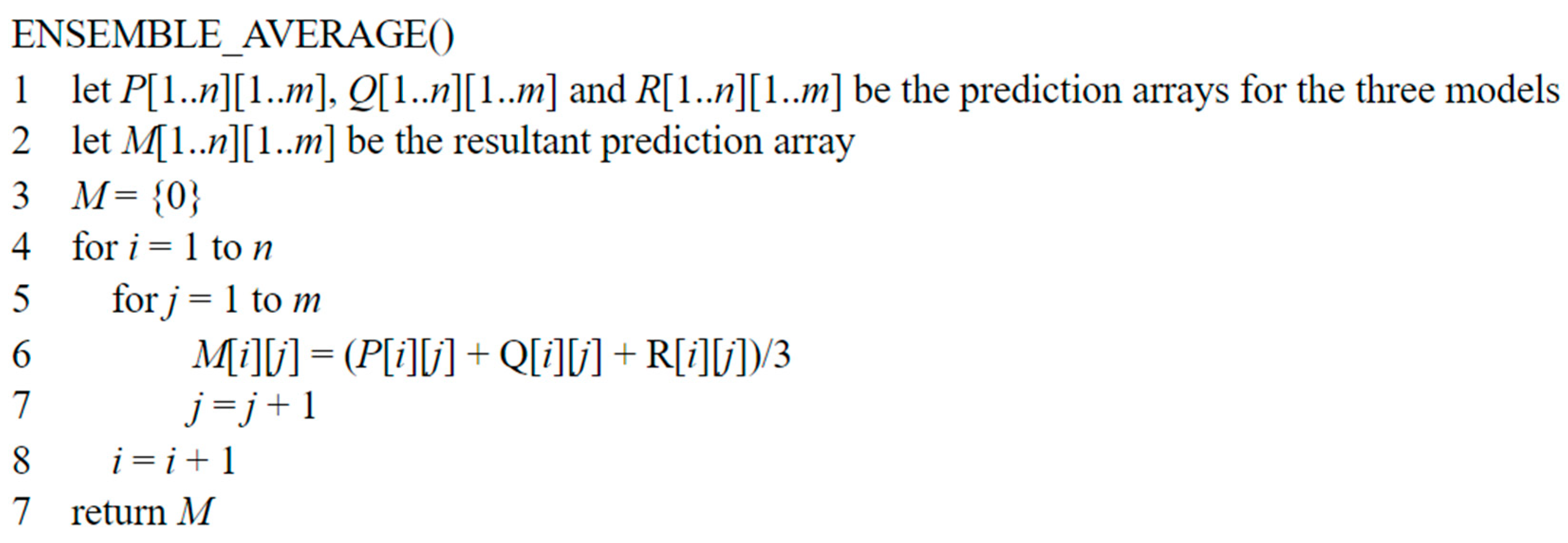
• The performance of many of the previously proposed model were not adequate, especially under challenging cases, e.g., identifying leaves with multiple diseases. In our research, we have used an ensemble of pre-trained deep learning models. The advantage of this is that our proposed model combines the predictions of three models and can perform well under challenging situations.
• We have deployed the proposed model in the form of a web application that serves as an easy-to-use system for I users. The user has to upload the leaf’s image on our web application, and the result is obtained in a couple of seco.

3. Methodology

In this section, we explain our step-wise methodology to elaborate the proposed model. Figure 4 shows the flow diagram that lists these main steps.

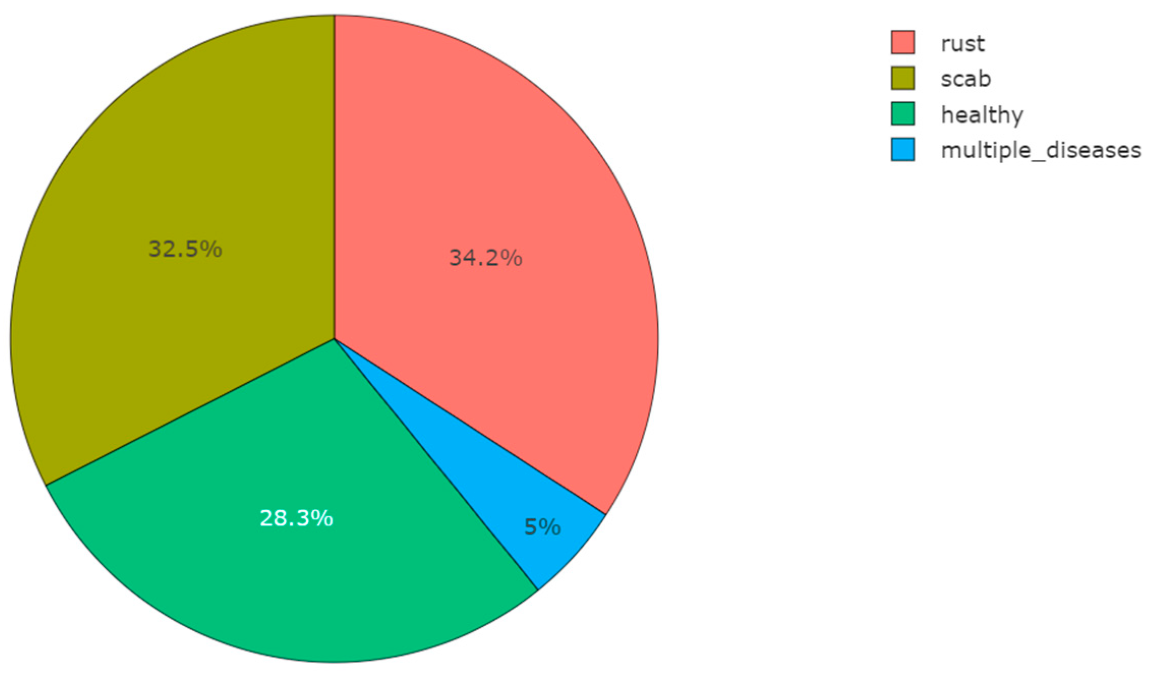
3.1. Dataset Collection

The dataset used in this research is an openly available dataset, which is a subset of the dataset created by the Plant Pathology and Plant-Microbe Biology Section of the Cornell University [41]. The original dataset contains 3651 high-grade images of apple leaves with various foliar diseases. The images are captured by hand in different scenarios such as variable lighting, different angles, different surfaces, etc., to represent a more general dataset that covers most possibilities. The dataset used in this research contains 3642 images of apple leaves distributed proportionally among four classes—cedar apple rust, multiple diseases, healthy leaves, and apple scab. The distribution of these four classes is shown in the pie chart represented in Figure 5. Out of the 3642 images available to us, only 5% of the plants have multiple diseases, i.e., having both scab and rust. The other three classes—healthy, cedar apple rust, and apple scab, are equivalent in proportion. The correct classification of apple leaves among the following four categories is the prime objective of this research.

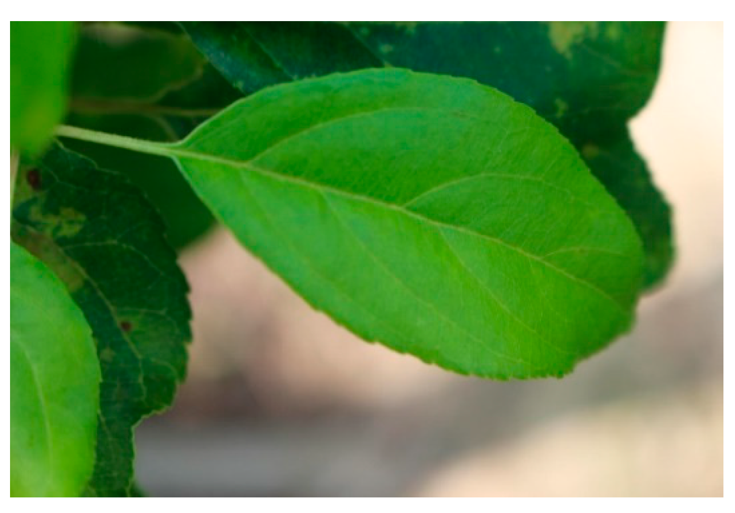
3.1.1. Healthy

It can be seen in Figure 6 that healthy leaves are entirely spotless and are green with no signs of any disease. Our dataset contains about 28.3% healthy leaves.

3.1.2. Apple Scab

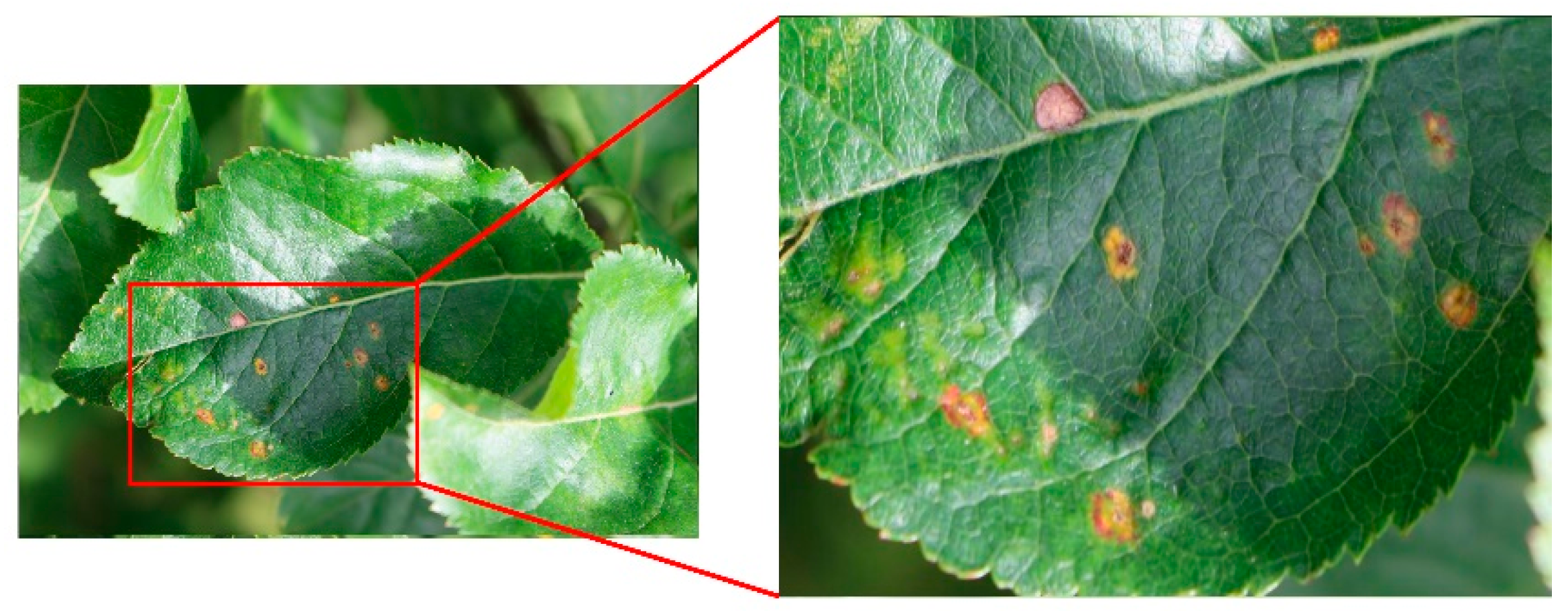
Figure 7 shows the leaf of an apple tree with apple scab disease. We can see that the leaves have brown spots/marks. A scab is often caused by a fungus that infects the leaves and the fruits, which makes the fruit unhealthy for eating. In our dataset, about 32.5% of images are of apple scab.

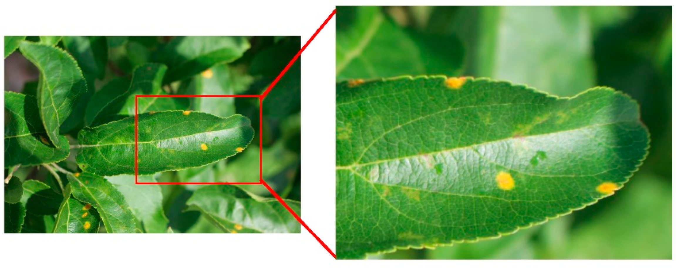
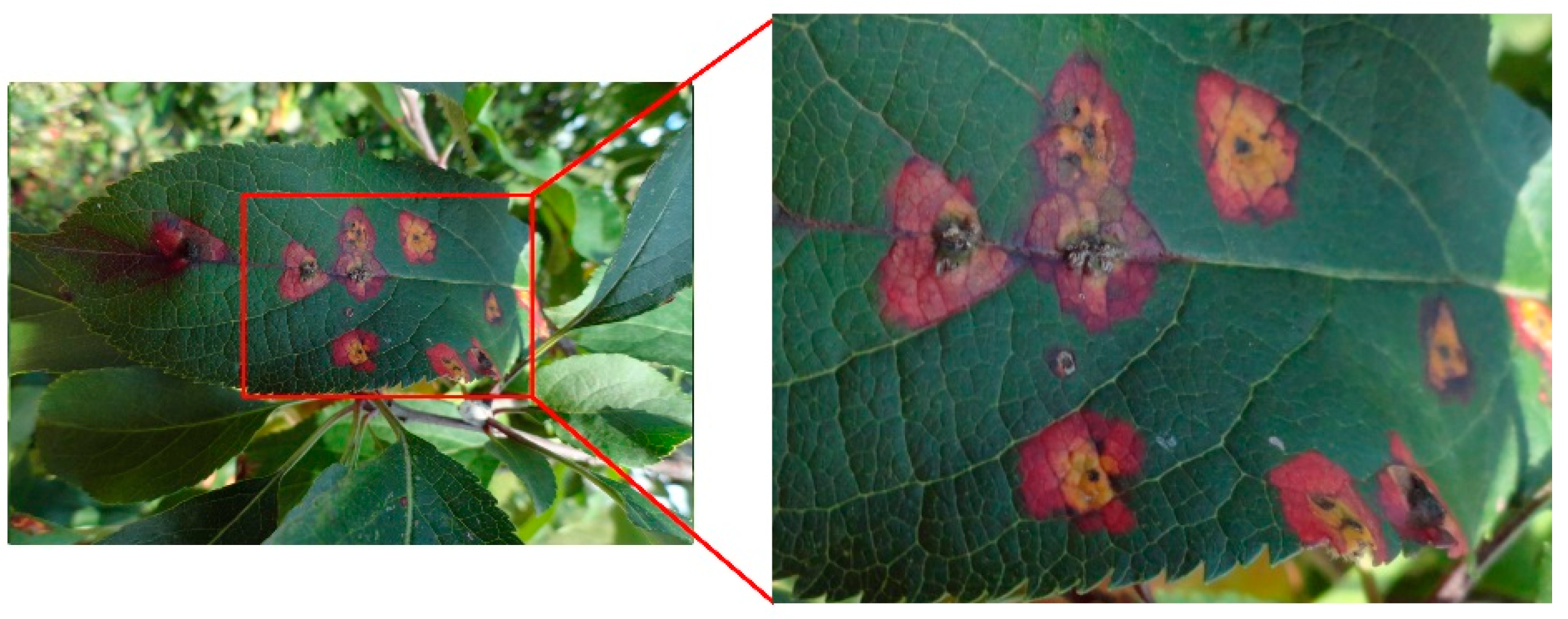
3.1.3. Cedar Apple Rust

Figure 8 shows the leaf of an apple tree having cedar apple rust. We can see that the leaves have dense yellowish marks. Rust is often caused in plants via a unique fungus named ‘rust fungus’. In our dataset, about 34.2% of images are of cedar apple rust.

3.1.4. Multiple Diseases

Leaves with multiple diseases show signs of having both apple scab, i.e., having brown spots, and cedar apple rust, i.e., having yellow marks as shown in Figure 9. The leaves are severely damaged in this case and are very difficult to treat. Our dataset has only 5% images from this class.

3.2. Image Augmentation

Image Augmentation refers to the process of augmenting our dataset to include more images by using various techniques such as: Rotation, Flipping, adding noise to the image, shear, shifts, etc. The advantages of this process are twofold. When our dataset is small, image augmentation can help us expand our dataset size without collecting new images manually. Image augmentation helps improve the performance of a model and helps build a better model by reducing the problem of overfitting in deep learning [42].

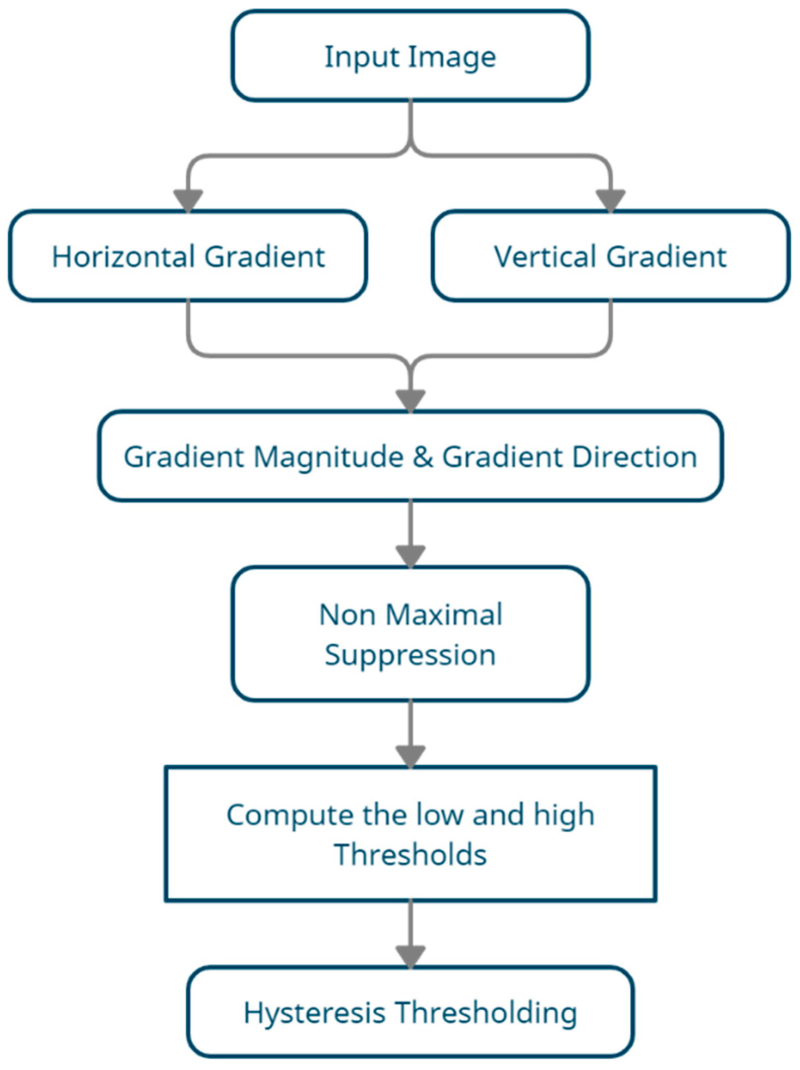
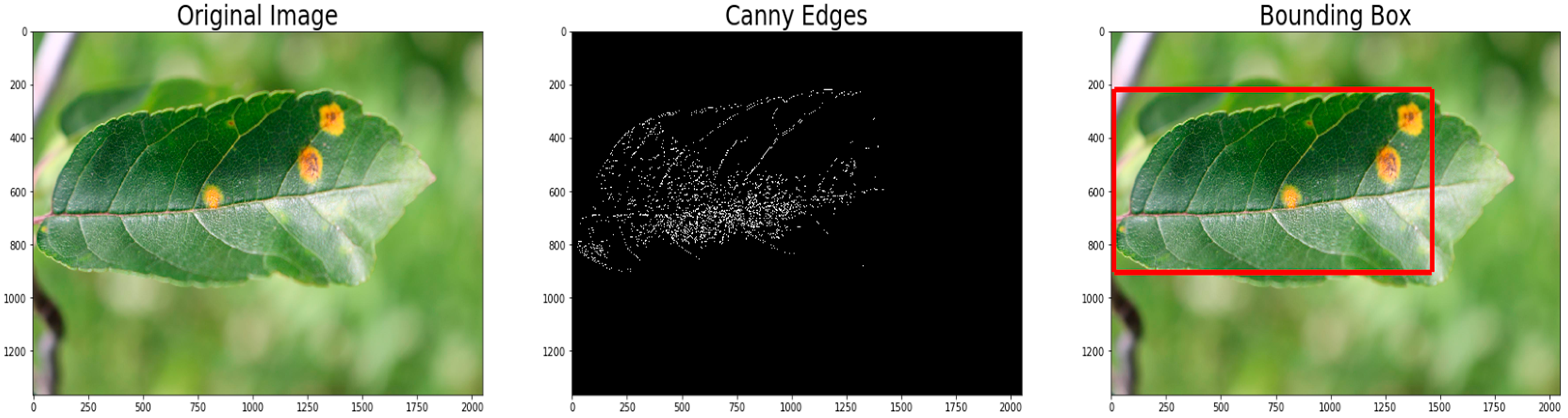
3.2.1. Canny Edge Detection

The edge detection process dramatically simplifies the analysis and training of images by significantly reducing the area under observation. At the same time, it retains the much-needed structural information of the picture contained in the boundaries. Canny Edge Detection [4] is a powerful computational approach for edge detection first introduced by John Canny. Canny Edge detection includes five steps, as shown in Figure 10.

The result of these five steps is a two-dimensional binary map (0 or 255) indicating the location of edges on the image. The result of applying this algorithm on the images of our dataset used in this work is shown in Figure 11.

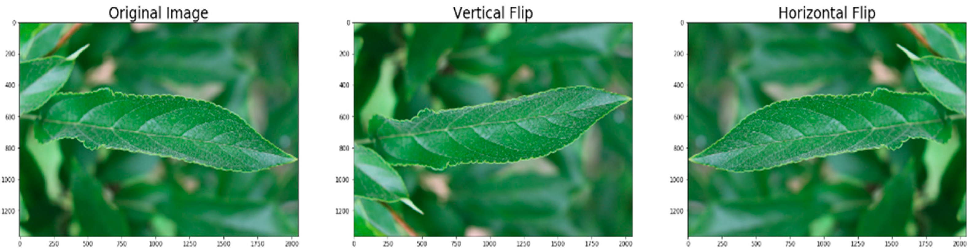
3.2.2. Flipping

Flipping is an operation that flips or upturns the order of rows (Horizontal Flipping) or the order of columns (Vertical Flipping) of the channels of an image. Consider an image with three channels of size (n × m) represented as A_ijk, where k is 3, meaning the red, green, and blue channels. The mathematical equations for flipping are shown below:

$$A_{ijk}=A_{i\left(m+1-j\right).k}$$

(1)

$$A_{ijk}=A_{\left(n+1-i\right).j.k}$$

(2)

Equation (1) represents vertical flipping, while Equation (2) represents horizontal flipping. The flipped images act as new images for our model and thus aid the overall process of building a robust model. An example of a flipped image for our dataset is shown in Figure 12.

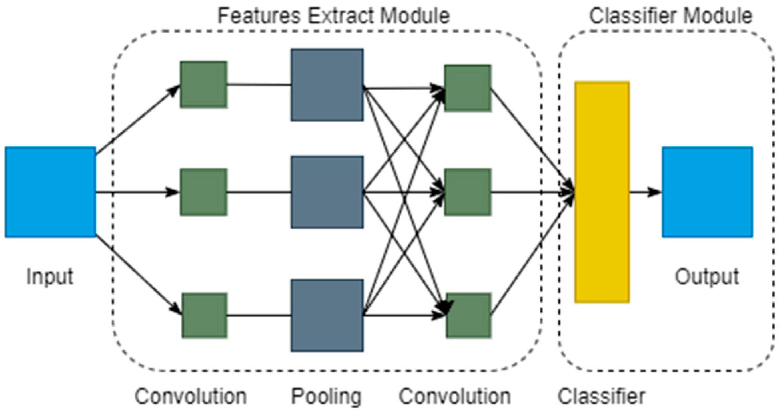
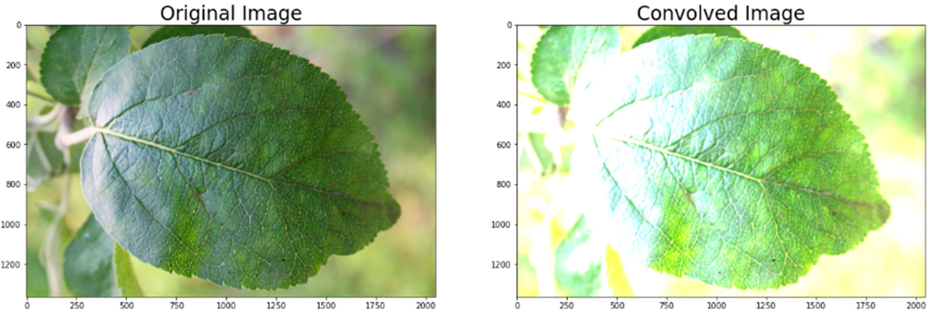
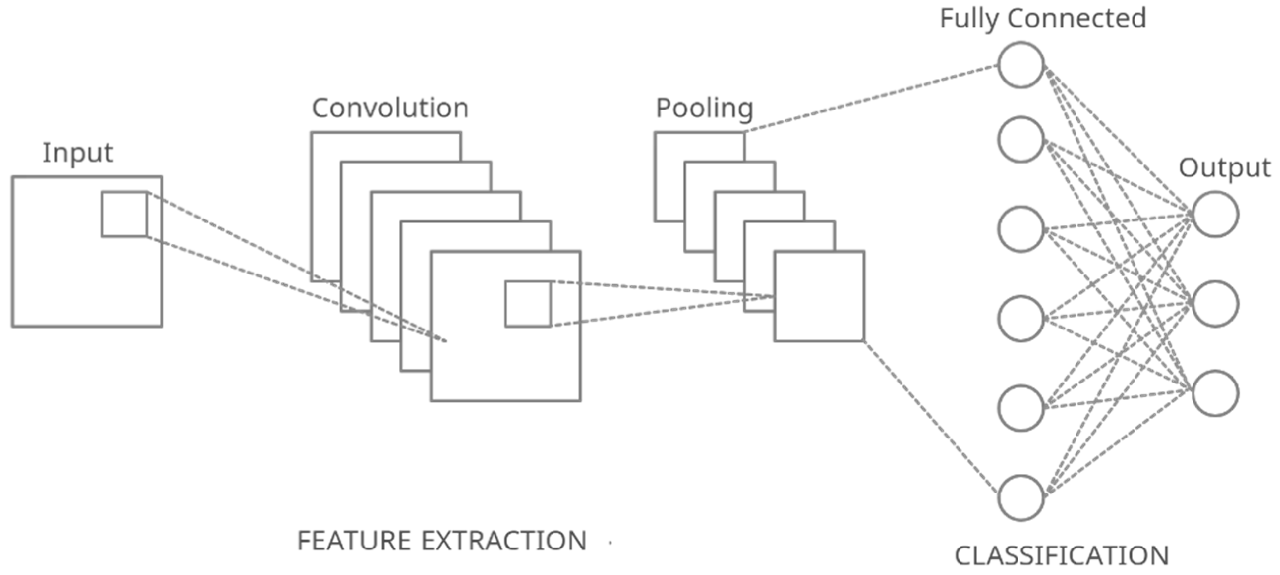
3.2.3. Convolution

Convolution is the process wherein a 2D matrix, or a mask, convolves or moves over an image step-by-step and calculates the dot product with each window along the way. The dot product involves the multiplication of corresponding cells of the mask and the window followed by adding all the obtained values. The size of the mask is usually of the order (1 × 1), (3 × 3), (5 × 5), or (7 × 7). Consider an image with N rows and M columns and the kernel having n rows and m columns, then the size of the final image will be N—n + 1 rows, and M—m + 1 columns. In mathematical terms, convolution can be represented as [43]:

$$O\left(i,j\right)={\displaystyle \sum }_{k=1}^m{\displaystyle \sum }_{l=1}^{n}I\left(i+k-1, j+l-1\right). K\left(k, l\right)$$

(3)

Here, i runs from 1 to N—n + 1 and j runs from 1 to M—m + 1. The output of the final image after convolution changes with the kernel values. The output of convolution in our case is shown in Figure 13.

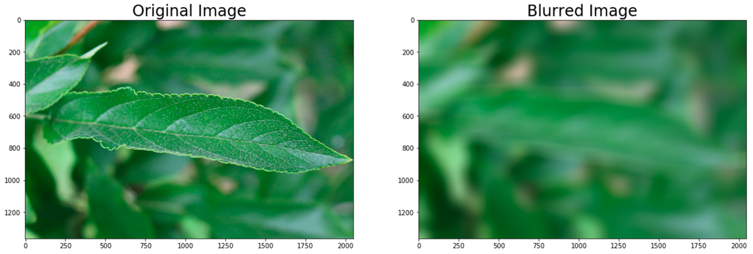
3.2.4. Blurring

In capturing an image for predicting its class, many defects can appear, such as blurred images, noise, poor contrast, etc. The most common of them is a blurred image, and it becomes difficult for a trained model to classify these images. Therefore, to make our model immune to such imperfections, we augment images by the process of Blurring. Blurring, in simple terms, is the addition of noise to an image to make it unclear. In the process of Blurring, one must be sure to change only minor details and not to over-add the noise. In our work, we have blurred our images by convolving them with a normalized block filter as shown [44] below:

$$K=\frac{1}{9}\left[\begin{array}{ccc}1& 1& 1\\ 1& 1& 1\\ 1& 1& 1\end{array}\right]$$

(4)

It takes the average of all the values present under the kernel area and the central value is replaced with the average value. The result of blurring on the image of our dataset is shown in Figure 14.

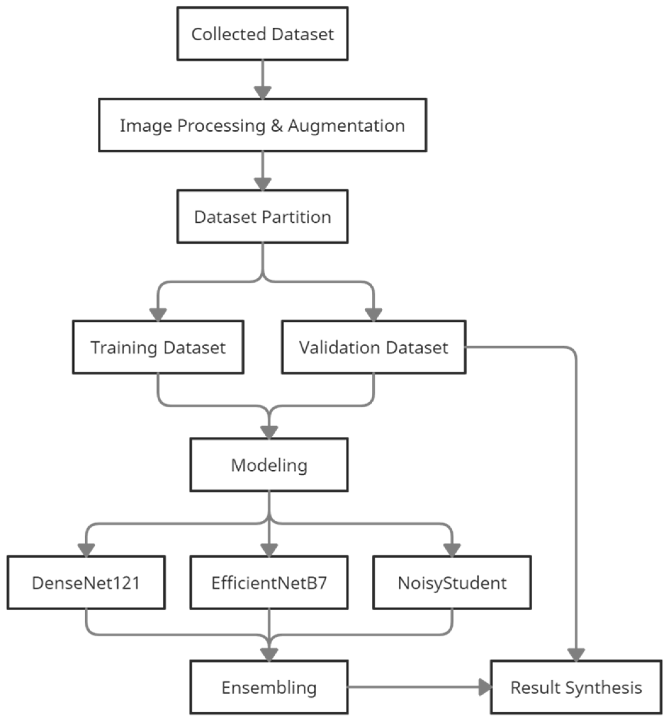
3.3. Dataset Partition

Our dataset contains a total of 3642 images of apple leaves. We divided these images in the ratio 17:3 between the training and validation dataset, i.e., 85% of the images were used for training, and the rest 15% of the images were used for validation. This means 3095 are the training images and 547 are validation images. We also carried out the process of Image Augmentation to elevate the size of the training dataset. Shuffling was carried out before splitting to get rid of any groups or collections already present in the dataset.

3.4. Modeling

3.4.1. Multiclass Classification

Multiclass classification is a subset of classification problems wherein there are more than two classes. In our study, there were four classes of apple leaf diseases that needed to be classified. The below figure illustrates the general structure of a CNN classifier. As we can see in Figure 15, an input is fed to the convolution stack, which extracts features via convolution, and the extracted features are then pooled to reduce the feature map size. The reduced feature map size is then mapped to a vector representing the final output classes for the problem via a dense layer.

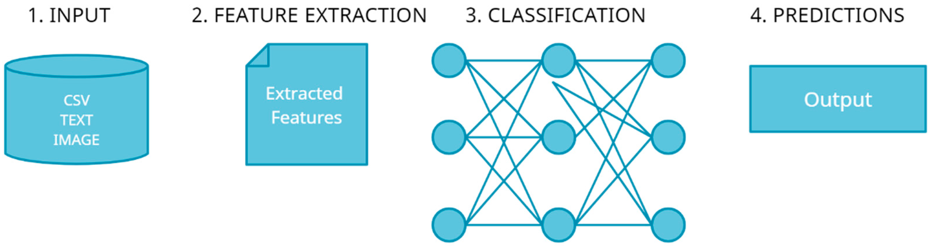
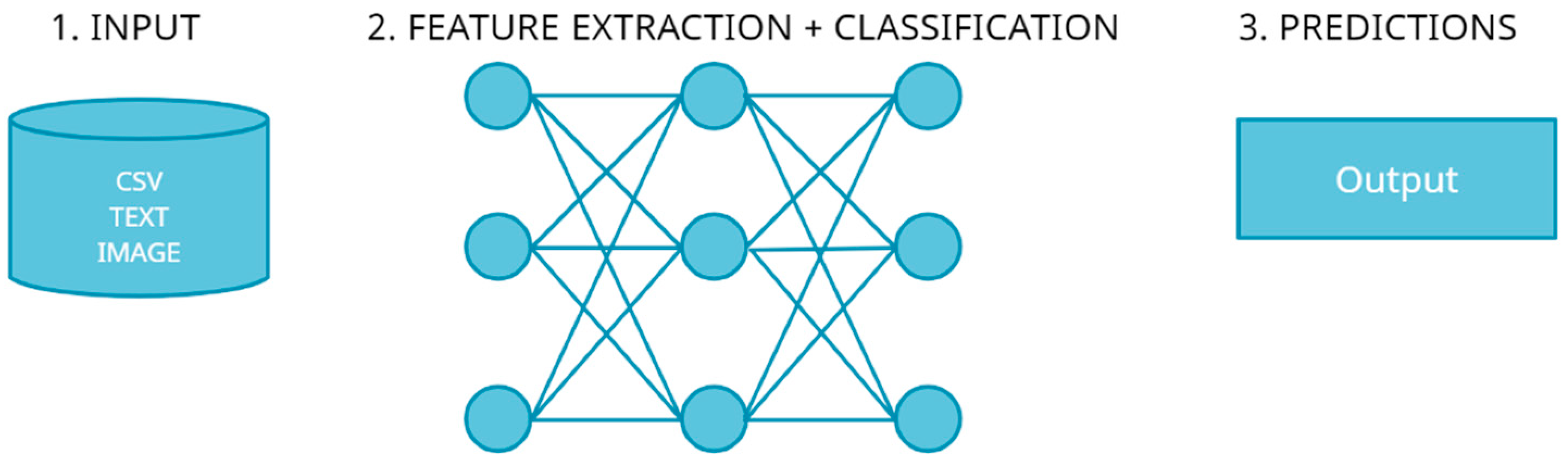
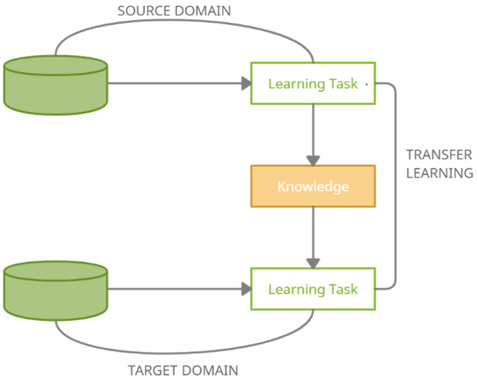
3.4.2. Transfer Learning

Transfer learning [17] is, in simple words, the process wherein the model trained for a task is used again as an initial point to train another model. Transfer learning is an essential mechanism in machine learning to resolve the fundamental dilemma of inadequate practice data. It tries to shift the information from the origin domain to the destination domain by slackening the premise that the practice data and the test data need to be comparable. The problem of inadequate data is unavoidable in many circumstances. The whole process of data collection and refining is cumbersome and requires time and patience. The learning process of a model using transfer learning is illustrated in Figure 16.

The main aim of deep transfer learning is to utilize knowledge gained in some other domain. Here, the source domain and the target domain need not be identically equivalent. In our research, we have designed an ensemble of three deep learning models, each of which is built upon a pre-trained base model, e.g., DenseNet.

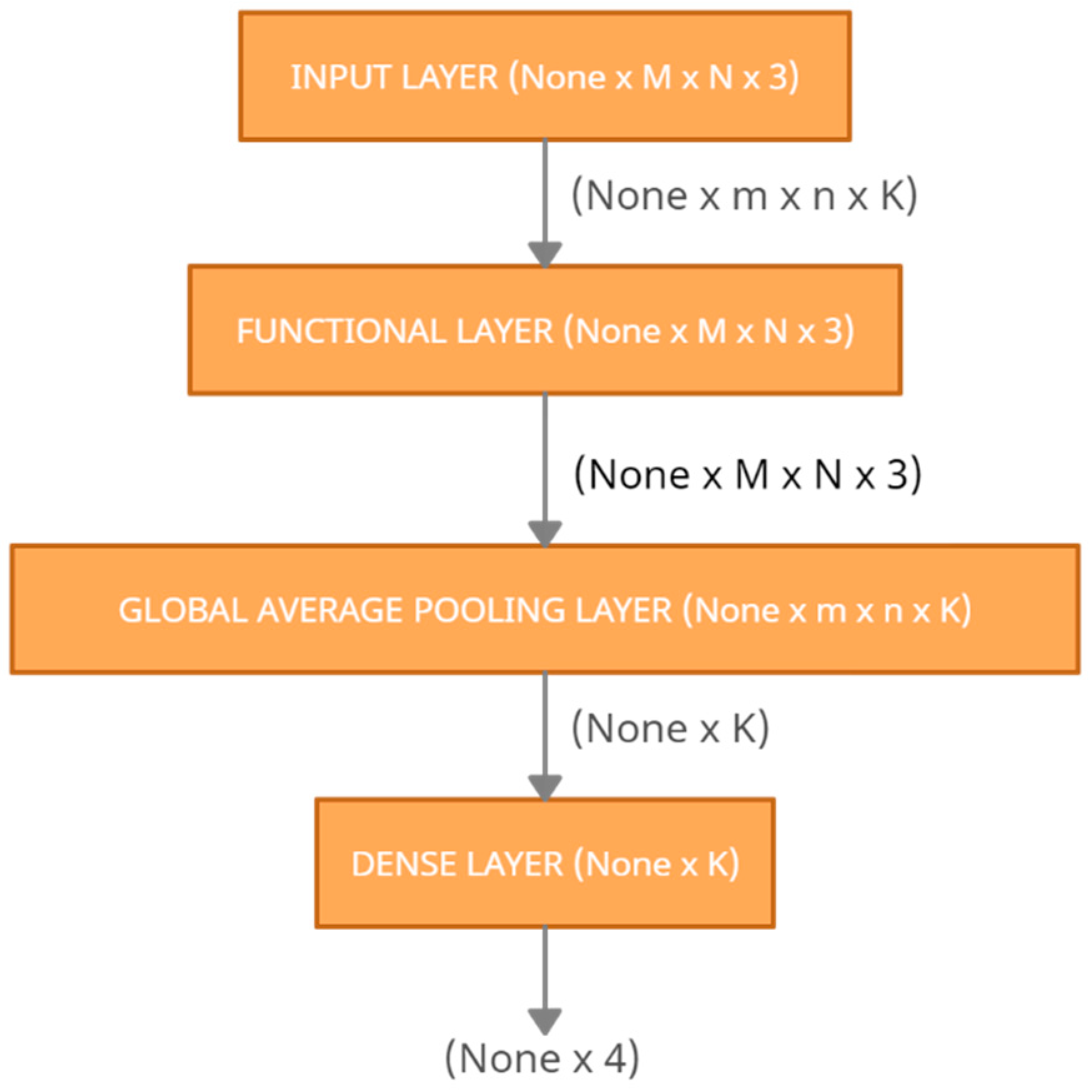
3.4.3. Model Structure

Each of the deep learning models that are part of the final ensemble assumes a general flow, as shown in Figure 17.

As it can be seen, the input layer assumes an image of size M × N × 3. In our case, the images are trimmed to the dimensions (512 × 512 × 3) before feeding it to the base pre-trained model. The functional layer represents the pre-trained model. These models are already trained using some other datasets, and we make use of their weights via transfer learning. The output of the functional layer is then fed to a Global Average Pooling layer [45]. The idea of introducing this layer is to reduce the size of the feature map to a 1D vector by averaging the values present in the pool (in our case, each m × n 2D vector). This layer outputs a one-dimensional vector which is fed to a fully connected dense layer. This final layer reduces the size to 4 classification categories and applies the SoftMax activation [46]. SoftMax function consumes a one-dimensional vector of Z values and outputs its normalized form, which consists of Z probabilities, each representing the probability of the classification falling in one of the Z classes. In our case, the value of Z is 4. The sum of all the probabilities equals 1 and the value of the SoftMax score lies between [0, 1] (0 and 1 inclusive). The target class with the highest probability is termed as the output of the whole classifier. Our models make use of the Adam Optimizer [47]. Adam optimization is an algorithm that iteratively updates network weights epoch by epoch. When compared to its counter algorithms, it is more effective and faster. During the training of the models, we kept the number of epochs to be 20 and the batch size per epoch as 128.

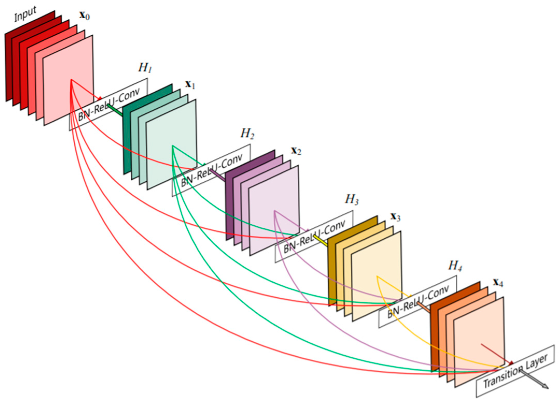
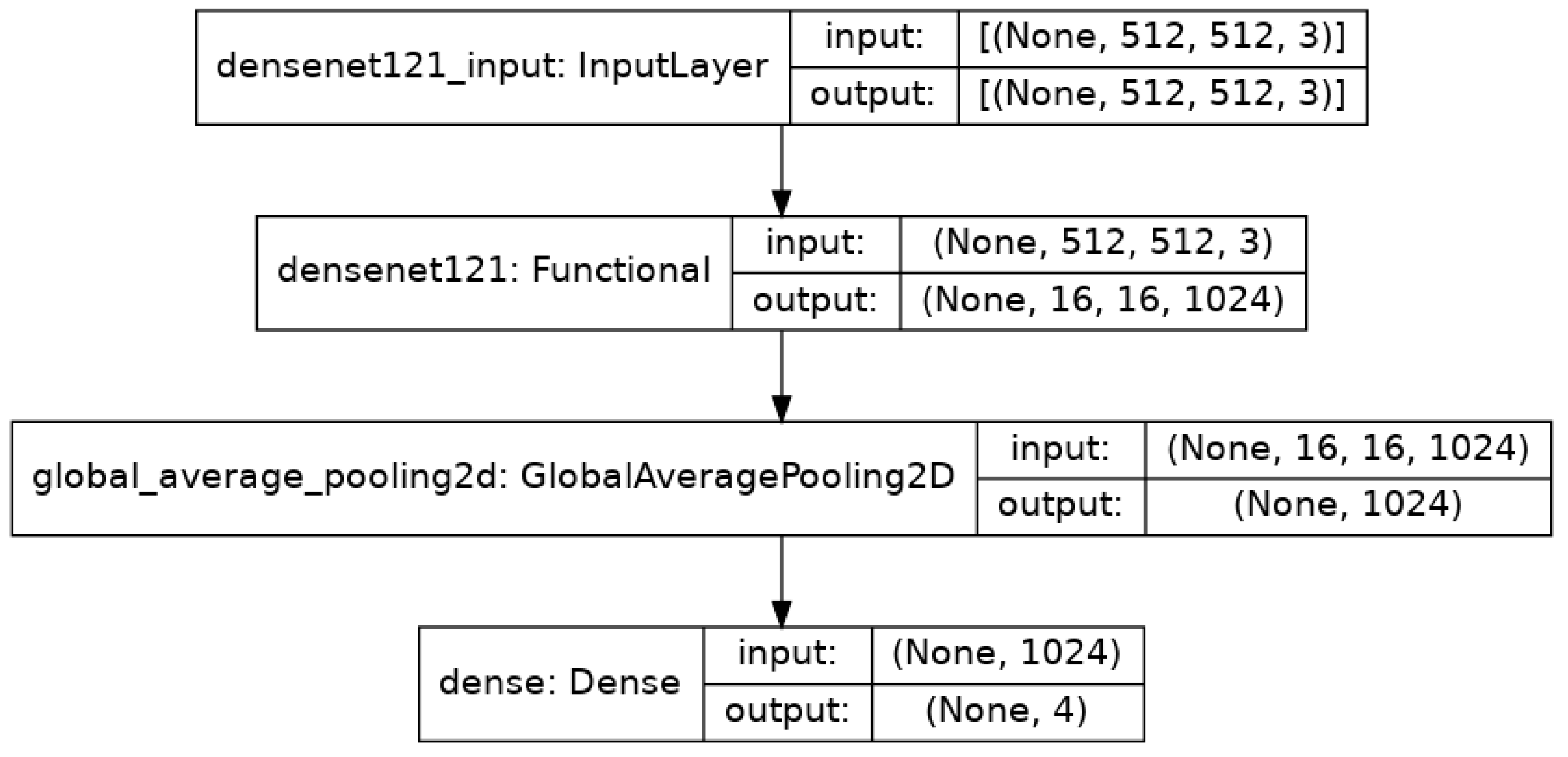
3.4.4. DenseNet121

Dense Convolutional Networks [14] (DenseNet) are a class of neural networks wherein each layer obtains inputs from every layer behind it and forwards its own feature map to all the subsequent layers. In a traditional convolutional network, the input passes through all the layers in a rather sequential fashion. In DenseNet, every layer acquires the knowledge of every preceding layer in a feed-forward fashion, as seen in Figure 18.

A DenseNet with L layers has L(L + 1)/2 connection compared to just L connections in a traditional convolution network. DenseNets have many captivating advantages: they mitigate the fading gradient obstacle, increase feature distribution, support feature reuse, and also considerably decrease the number of parameters. Since each layer receives input from every layer behind it, DenseNets are usually more compact since they extract almost the same number of features in a relatively smaller-sized network.

In this work, we have used the DenseNet121 variant of DenseNet pre-trained on ImageNet [48] dataset. The ‘121′ in DenseNet121 refers to the number of layers that include trainable weights leaving the locked layers. Figure 19 represents the structure of our model that provides for the pre-trained DenseNet121 model.

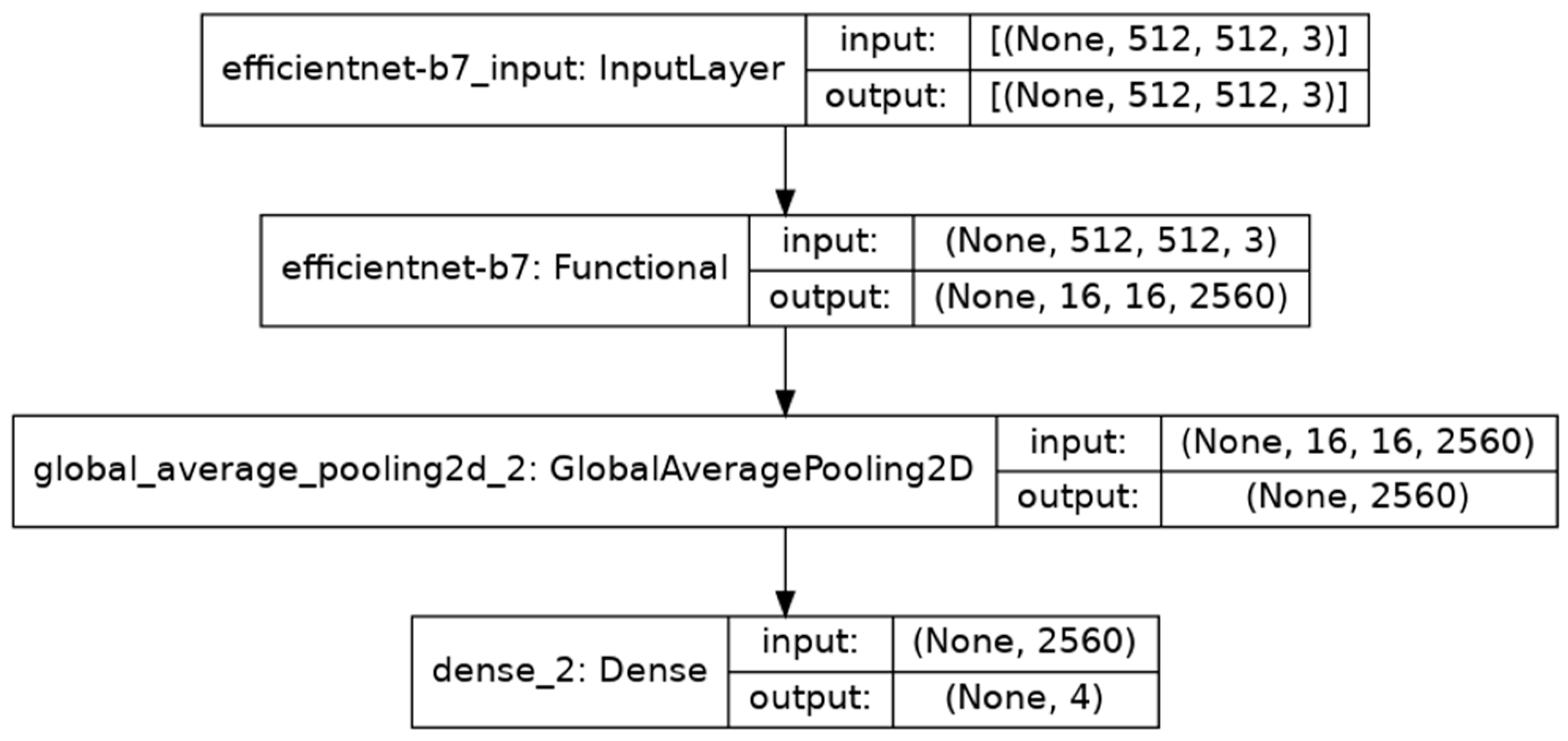
3.4.5. EfficientNet

EfficientNet [15] is a type of convolutional neural network that employs a unique scaling method that evenly scales each dimension, i.e., width, depth, and resolution adopting a compound coefficient.

Scaling is a major concern for most data science practitioners across the world. Scaling of a network is performed mainly across three dimensions—width, depth, and resolution. However, it has been observed that scaling initially does increase accuracy, but the spike in accuracy saturates gradually with scaling [15]. In other words, traditional ConvNets may not perform scaling ‘efficiently’. EfficientNets simplifies this problem of scaling by something known as Compound Scaling [49]. In this technique, a Compound Coefficient is used to scale the network uniformly across the three dimensions. The graph in Figure 20 shows how EfficientNet outperforms various other state-of-the-art models on the ImageNet dataset classification task and does not saturate when the number of trainable parameters is increased.

For our research, we used the EfficientB7 model pre-trained on the ImageNet dataset. Figure 21 represents the structure of our model that includes the pre-trained EfficientNetB7 model.

3.4.6. EfficientNet Noisy Student

EfficientNet Noisy Student [16] implements the idea of Noisy Student Training. In this process, the EfficientNet model is initially trained on the ImageNet dataset of labeled images, and then the predictions of this model are used as pseudo-labels for the remaining unlabeled images. This process is repeated back and forth with the injection of noise so that the final model generalizes better than the initial models. EfficientNet Noisy student has outperformed EfficientNet on several tasks since its knowledge base includes visual-rich representations gained by training over noisy images. It can be seen in the graph in Figure 20 that NoisyStudent outperforms all other EfficientNet variants in terms of accuracy on ImageNet task classification.

In our research, we have used pre-trained EfficientNetB7 having noisy student weights. Figure 22 below represents the structure of our model that makes use of pre-trained EfficientNet Noisy Student.

3.5. Ensembling

A disadvantage of using predictions of multiple deep learning classifiers is that they have high variance. Since each classifier is trained individually with different data being fed to it in each epoch, each of them updates their weight in isolation and thus present different results on the task of classifying the same image. A simple approach to tackle the above problem is to combine the predictions from all the classifiers somehow. This shall reduce the variance, and the ensemble will generalize well compared to the individual models. The ensemble approach used in this research is Model Averaging [18]. In this approach, every classifier’s contribution remains equal to compute the final prediction. The algorithm used for Model Averaging is shown in Figure 23. Unweighted averaging might be a reasonable ensemble for similar base learners of comparable performance [50]. To predict class probability, the result is computed by calculating the argmax of the summed probabilities for each class.

4. Experimental Results and Analyses

In this section, the experimental setup is first introduced, followed by the description of various performance metrics, analysis and comparison of our results, a description of computational resources, and information about the model deployment.

4.1. Experimental Setup

We developed and trained our model using Python3. Along with Python, we leveraged the functionalities of various frameworks and libraries such as Keras, Tensorflow, Pandas, Numpy for our purpose. We used Kaggle [51] that offers free access to TPUs (Tensor Processing Units) for a fixed number of hours per week [52]. Tensor Processing Units, developed by Google, are custom-developed application-specific integrated circuits (ASICs) to hasten machine learning and deep learning-related work. TPU v3-8 provides 128 GB of RAM and 19.6 GB of disk space along with eight computational cores. We used tf.data dataset [53] api of Tensorflow to create a dataset from the input images and apply transformations to the data. To transform the dataset, we mapped our dataset to functions for Flipping, Rotation, Blurring, etc. We loaded our model using the sequential class of Keras and specified weights as image net. While loading the model, functional calls to the required metrics such as: precision, F1, etc., were selected. We ran around 20 epochs with 12 steps per epochs for a Batch size of 128. The starting value of the learning rate was kept as 1 × 10⁻⁵. The results were obtained via the history object obtained after fitting our models. The visualization of results was achieved by using the Seaborn [54] library offered by Python. Finally, the ensembling was carried out by averaging the corresponding cell values for the prediction matrices of the trained models.

4.2. Performance Metrics

The performance of our proposed model and individual pre-trained models are assessed by four metrics, i.e., Validation Accuracy, positive predictive value (PPV), also known as Precision, Recall, and F1-Score. In addition to these, confusion matrices are shown for each model, and the necessary conclusions are drawn. The plots for Accuracy vs. Epochs have also been presented for the pre-trained models.

Accuracy, in simple words, is the number of accurate predictions made concerning the total predictions made by a model. [55].

$$Accuracy=\frac{Number of correct predictions}{Total number of predictions}$$

(5)

Precision is the ratio of the number of correct positive results divided by the number of positive results predicted by the classifier [55].

$$Precision=\frac{TruePositives}{TruePositives+FalsePositives}$$

(6)

Recall is the ratio of the number of correct positive results divided by the number of all relevant samples (all samples that should have been identified as positive) [55].

$$Recall=\frac{ TruePositives}{TruePositives+FalseNegatives}$$

(7)

F1-Score is the harmonic mean of Precision and Recall [55].

$$F1=\frac{2}{\frac{1}{precision}+\frac{1}{recall}}$$

(8)

The value of the F1-score lies in the range of [0, 1]. A higher value of F1 signifies a better balance in Precision and Recall. In other words, the higher value of this metric indicates a better and robust model.

4.3. Performance Benchmarking

In this section, we present the results of our proposed model alongside the results of the pre-trained models.

Table 1. Accuracy of the pre-trained and proposed model at various split ratios.

Split	DenseNet121	EfficientNetB7	NoisyStudent	Our Model
0.10	0.9398	0.9416	0.9095	0.9344
0.15	0.9526	0.9562	0.9124	0.9625
0.20	0.9511	0.9506	0.9233	0.9499
0.25	0.9414	0.9471	0.8991	0.9211
0.30	0.9232	0.9376	0.9091	0.9301

shows the accuracy of the pre-trained models and our proposed model at different values of the train-test split. It is observed that DenseNet121 and EfficientNetB7 tend to achieve the best accuracy at a 0.15 split ratio, but EfficientNet NoisyStudent classifies most accurately at a 0.20 split ratio. Our proposed model achieves an accuracy of 96.25% on a 0.15 split ratio. Figure 24 shows the plots of Accuracy vs. Epochs for the pre-trained models and our proposed model.

Table 2. Precision of pre-trained models and proposed model at various split ratios.

Split	DenseNet121	EfficientNetB7	NoisyStudent	Our Model
0.10	0.8432	0.8637	0.8344	0.8555
0.15	0.8637	0.8901	0.8479	0.9091
0.20	0.9496	0.8871	0.8544	0.8963
0.25	0.8598	0.8388	0.8282	0.8446
0.30	0.8876	0.8876	0.8298	0.8991

and

Table 3. Recall of pre-trained models and proposed model at various split ratios.

Split	DenseNet121	EfficientNetB7	NoisyStudent	Our Model
0.10	0.8442	0.8637	0.8344	0.8518
0.15	0.8637	0.8961	0.8429	0.8977
0.20	0.9496	0.8870	0.8542	0.8951
0.25	0.8221	0.8388	0.8238	0.8331
0.30	0.8806	0.8806	0.8301	0.8881

show the precision and recall of the pre-trained models and our proposed model at different values of train-test split. It is observed that the value of recall and precision of our proposed model is higher than the pre-trained models. The best values are obtained at a 0.15 split ratio.

Table 4. F1-Scores of pre-trained models and proposed model at various split ratios.

Split	DenseNet121	EfficientNetB7	NoisyStudent	Our Model
0.10	0.8442	0.8637	0.8329	0.8497
0.15	0.8637	0.8922	0.8453	0.9098
0.20	0.9496	0.8871	0.8576	0.8732
0.25	0.8560	0.8382	0.8249	0.8490
0.30	0.8839	0.8839	0.8290	0.8987

shows the F1 scores of the pre-trained models and our proposed model at different values of the train-test split. The table proves that our model beats the F1 scores of the pre-trained models at all split values. The F1-score is highest at a 0.15 split with a value of 0.9098.

Figure 25 shows that all the three pre-trained models perform well in the case of healthy, scab, and rust classes, but for images with multiple diseases, the performance is not up to the mark. On average, DenseNet121 only classifies 62 images correctly out of 100 images with multiple diseases, while this number is 69 for EfficientNetB7 and 54 for EfficientNet NoisyStudent. In the proposed model, we ensemble the predictions of the three models—DenseNet121, EfficientNetB7, and EfficientNet NoisyStudent via Model Averaging. This will reduce the variance across the predictions of the three models. The performance of our proposed model on this dataset can be viewed from the confusion matrix shown in Figure 25. It is observed that the proposed model outperforms all three models in a case, when the leaf has multiple diseases. On average, the proposed model correctly predicts 90 images as multiple diseases out of 100 images.

Table 5. Comparison of previous models with our model.

Model	Accuracy
DenseNet	0.9260
GoogleNet	0.9530
EfficientNetB7	0.9562
ResNet20	0.9370
VggNet-16	0.9400
Our Model	0.9625

shows the performance of GoogleNet, ResNet, VggNet-16, and DenseNet on the same classes we trained our proposed model for [35].

It is clear from Table 5 that our model outperforms various state-of-the-art CNN models on the given dataset in terms of accuracy.

4.4. Computational Resources

According to the theory of computation, the most straightforward computational resources are the time taken for calculation, the number of parameters involved, and the memory required. In this section, we have summarized the computational requirements of our proposed model based on these three factors. The TPU provided by Kaggle gives 128 GB of memory, out of which our model’s peak usage was 16 GB of memory. This was the case when the batch size was 128. The training time for our model ranges from 31.6 min to 42.7 min, which depends upon factors such as: available free memory, network bandwidth, etc. The prime parameters involved in the computation of our proposed model are batch size, number of epochs, and steps per epoch. The values for these factors have been given in Section 4.1. It is observed that the computational time is directly proportional to the batch size and the steps per epoch.

4.5. Model Deployment

We have deployed our proposed model using a web application. We have named our web application Leaviify. This application aims to serve as an easy-to-use platform for people to leverage the functionality of our model.

4.5.1. Overview

To use our system, the user has to visit our web application and upload the image of the apple leaf for which he wants to check the class. On clicking the upload button, the image is sent to the backend, where it is fed to our model, and the result is showed to the user. Figure 26 shows the snapshot of our web application which depicts the above-foresaid process. The entire code of our web application is available at https://github.com/prakhar070/apple-disease-detection (accessed on 20 April 2021) [56].

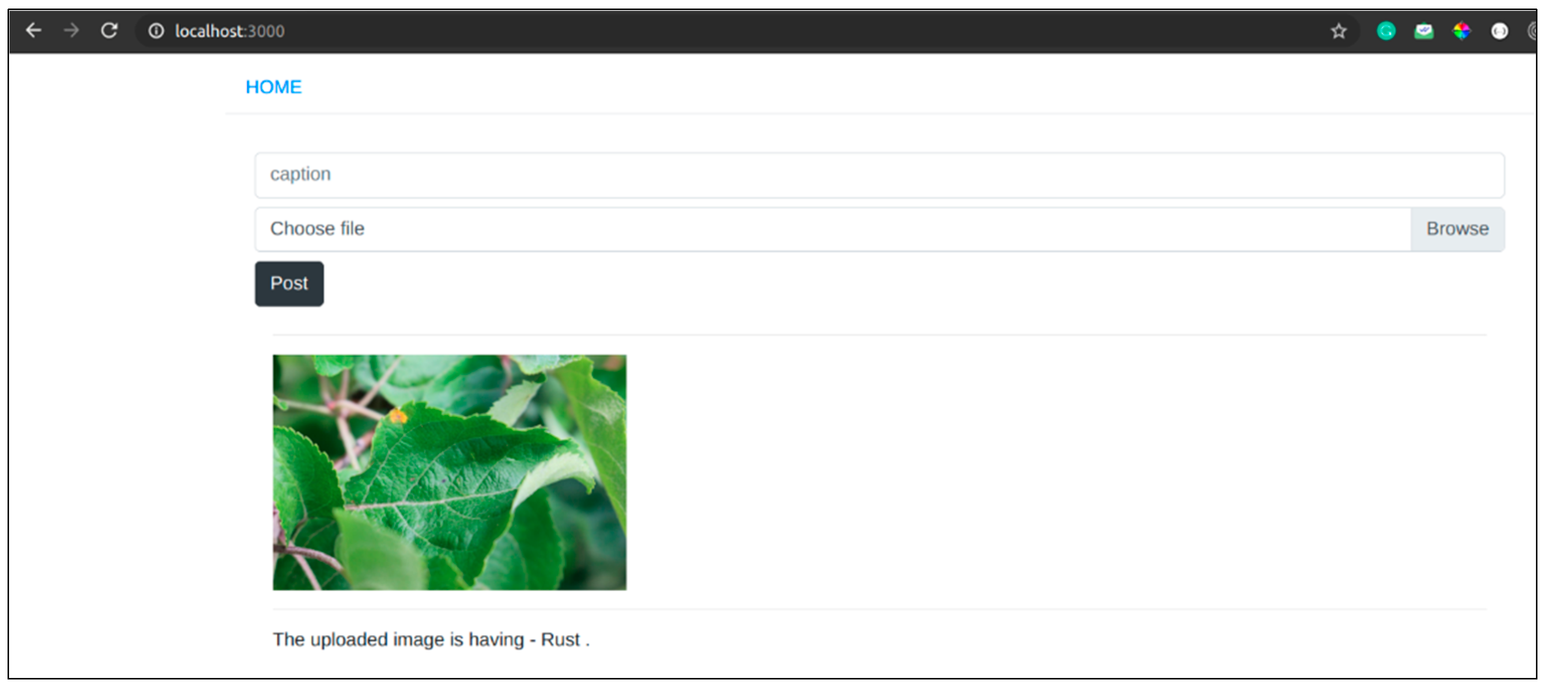
4.5.2. Web Application Work Flow

The working algorithm of our system is summarized in the following points—

• User visits our web application and uploads the image of apple leaf. All this takes place at the frontend.
• The image uploaded is then sent to the backend, where it is fed to the CNN model. At the backend, we have stored the weights of our proposed model in the form of an HDF5 file [57]. The model is loaded from this HDF5 file. Before feeding the image to the model, the image is first trimmed into the required shape of 512 × 512.
• The result returned by our model is a NumPy array of size (4,1), which includes the probability of the four classes. The class with the maximum probability is extracted.
• The results are shown to the user at the frontend, and the image is stored in our database to enhance our model.

4.5.3. Technologies Used

Our web application has a simple frontend designed using Javascript, CSS, and HTML. The backend of our application uses Ruby on Rails which is a server-side web application framework. The backend of our application maps the frontend to our deep learning model. The proposed model uses technologies such as Python, Keras, Tensorflow, NumPy and Pandas, etc. to store the images in a database to make them available for future training; we have used MySQL, an open-source RDBMS.

5. Conclusions

In this paper, we proposed an ensemble of pre-trained deep learning models—DenseNet121, EfficientNetB7, and EfficientNet NoisyStudent—and analyzed their performance on a dataset containing images of apple leaves. The dataset includes 3642 apple leaves with four classes—apple scab, apple cedar rust, multiple diseases, and healthy. The major limitation of this work that we focused on only four classes of the images that only relate to two foliar diseases. We also analyzed and compared its performance with various state-of-the-art models and concluded that it outperformed all those models, which are trained on the same dataset. We also examined the scores of the three models individually for multiple metrics such as accuracy, precision, recall, F1, etc. Finally, we ensembled the predictions of the three models via averaging. Our final model achieves an accuracy of 96.25% on the validation dataset. With this accuracy in the picture, farmers can use this approach to automate disease classification in apple trees. This will save not only time, but also money since the need for experts can be minimized in certain situations. We also deployed the proposed model via an easy-to-use web application, so that naive users find it easy to use our model. This application is very useful for farmers in far remote areas, where the services of plant pathologists are not easily accessible. In future work, we aim to expand the classes under focus for our model to include other categories of foliar diseases. Additionally, we intend to widen our dataset to include more images of apple leaves to build better models for future.

References

- Apple. Wikipedia. 2021. Available online: https://en.wikipedia.org/wiki/Apple (accessed on 22 April 2021).
- Jordan, M.I.; Mitchell, T.M. Machine Learning: Trends, Perspectives, and Prospects. Science 2015, 349, 255–260. [Google Scholar] [CrossRef]
- Badage, A. Crop disease detection using machine learning: Indian agriculture. Int. Res. J. Eng. Technol. 2018, 5, 866–869. [Google Scholar]
- Canny, J. A Computational Approach to Edge Detection. IEEE Trans. Pattern Anal. Mach. Intell. 1986, PAMI-8, 679–698. [Google Scholar] [CrossRef]
- Korkut, U.B.; Göktürk, Ö.B.; Yildiz, O. Detection of Plant Diseases by Machine Learning. In Proceedings of the 2018 26th Signal Processing and Communications Applications Conference (SIU), Izmir, Turkey, 2–5 May 2018; pp. 1–4. [Google Scholar]
- Noble, W.S. What Is a Support Vector Machine? Nat. Biotechnol. 2006, 24, 1565–1567. [Google Scholar] [CrossRef]
- Quinlan, J.R. Simplifying Decision Trees. Int. J. Man-Mach. Stud. 1987, 27, 221–234. [Google Scholar] [CrossRef] [Green Version]
- Huang, Y.; Li, L. Naive Bayes Classification Algorithm Based on Small Sample Set. In Proceedings of the 2011 IEEE International Conference on Cloud Computing and Intelligence Systems, Beijing, China, 15–17 September 2011; pp. 34–39. [Google Scholar]
- LeCun, Y.; Bengio, Y.; Hinton, G. Deep Learning. Nature 2015, 521, 436–444. [Google Scholar] [CrossRef]
- Kumar, E.P.; Sharma, E.P. Artificial neural networks-a study. Int. J. Emerg. Eng. Res. Technol. 2014, 2, 143–148. [Google Scholar]
- Pardede, H.F.; Suryawati, E.; Sustika, R.; Zilvan, V. Unsupervised Convolutional Autoencoder-Based Feature Learning for Automatic Detection of Plant Diseases. In Proceedings of the 2018 International Conference on Computer, Control, Informatics and Its Applications (IC3INA), Tangerang, Indonesia, 1–2 November 2018; pp. 158–162. [Google Scholar]
- Howard, A.G. Some Improvements on Deep Convolutional Neural Network Based Image Classification. arXiv 2013, arXiv:1312.5402. [Google Scholar]
- Boulent, J.; Foucher, S.; Théau, J.; St-Charles, P.-L. Convolutional Neural Networks for the Automatic Identification of Plant Diseases. Front. Plant Sci. 2019, 10, 941. [Google Scholar] [CrossRef] [Green Version]
- Huang, G.; Liu, Z.; Van Der Maaten, L.; Weinberger, K.Q. Densely Connected Convolutional Networks. In Proceedings of the 2017 IEEE Conference on Computer Vision and Pattern Recognition (CVPR), Honolulu, HI, USA, 21–26 July 2017; pp. 2261–2269. [Google Scholar]
- Tan, M.; Le, Q. EfficientNet: Rethinking Model Scaling for Convolutional Neural Networks. In Proceedings of the International Conference on Machine Learning, Long Beach, CA, USA, 24 May 2019; pp. 6105–6114. [Google Scholar]
- Xie, Q.; Luong, M.-T.; Hovy, E.; Le, Q.V. Self-Training With Noisy Student Improves ImageNet Classification. In Proceedings of the 2020 IEEE/CVF Conference on Computer Vision and Pattern Recognition (CVPR), Seattle, WA, USA, 13–19 June 2020; pp. 10684–10695. [Google Scholar]
- Tan, C.; Sun, F.; Kong, T.; Zhang, W.; Yang, C.; Liu, C. A Survey on Deep Transfer Learning. In Artificial Neural Networks and Machine Learning-ICANN 2018 Lecture Notes in Computer Science; Kůrková, V., Manolopoulos, Y., Hammer, B., Iliadis, L., Maglogiannis, I., Eds.; Springer: Cham, Germany, 2018; Volume 11141. [Google Scholar] [CrossRef] [Green Version]
- Steel, M.F.J. Model Averaging and Its Use in Economics. J. Econ. Lit. 2020, 58, 644–719. [Google Scholar] [CrossRef]
- Selvaraj, M.G.; Vergara, A.; Ruiz, H.; Safari, N.; Elayabalan, S.; Ocimati, W.; Blomme, G. AI-Powered Banana Diseases and Pest Detection. Plant Methods 2019, 15, 92. [Google Scholar] [CrossRef]
- Early Detection and Classification of Plant Diseases with Support Vector Machines Based on Hyperspectral Reflectance. Comput. Electron. Agric. 2010, 74, 91–99. [CrossRef]
- Sinha, A.; Shekhawat, R.S. Review of Image Processing Approaches for Detecting Plant Diseases. IET Image Process. 2019, 14, 1427–1439. [Google Scholar] [CrossRef]
- Ramesh, S.; Hebbar, R.; Niveditha, M.; Pooja, R.; Shashank, N.; Vinod, P.V. Plant Disease Detection Using Machine Learning. In Proceedings of the 2018 International Conference on Design Innovations for 3Cs Compute Communicate Control (ICDI3C), Bangalore, India, 25–28 April 2018; pp. 41–45. [Google Scholar]
- Yang, X.; Guo, T. Machine Learning in Plant Disease Research. Eur. J. Biomed. Res. 2017, 3, 6–9. [Google Scholar] [CrossRef] [Green Version]
- Mohanty, S.P.; Hughes, D.P.; Salathé, M. Using Deep Learning for Image-Based Plant Disease Detection. Front. Plant Sci. 2016, 7. [Google Scholar] [CrossRef] [PubMed] [Green Version]
- Saleem, M.H.; Potgieter, J.; Arif, K.M. Plant Disease Detection and Classification by Deep Learning. Plants 2019, 8, 468. [Google Scholar] [CrossRef] [Green Version]
- Goncharov, P.; Ososkov, G.; Nechaevskiy, A.; Uzhinskiy, A.; Nestsiarenia, I. Disease Detection on the Plant Leaves by Deep Learning. In Proceedings of the International Conference on Neuroinformatics, Moscow, Russia, 8–12 October 2018; Kryzhanovsky, B., Dunin-Barkowski, W., Redko, V., Tiumentsev, Y., Eds.; Advances in Neural Computation, Machine Learning, and Cognitive Research II. Springer International Publishing: Cham, Germany, 2019; pp. 151–159. [Google Scholar]
- Sun, J.; Yang, Y.; He, X.; Wu, X. Northern Maize Leaf Blight Detection Under Complex Field Environment Based on Deep Learning. IEEE Access 2020, 8, 33679–33688. [Google Scholar] [CrossRef]
- Vine Disease Detection in UAV Multispectral Images Using Optimized Image Registration and Deep Learning Segmentation Approach. Comput. Electron. Agric. 2020, 174, 105446. [CrossRef]
- Identification of Rice Diseases Using Deep Convolutional Neural Networks. Neurocomputing 2017, 267, 378–384. [CrossRef]
- Amara, J.; Bouaziz, B.; Algergawy, A. A Deep Learning-Based Approach for Banana Leaf Diseases Classification. In Datenbanksysteme für Business, Technologie und Web (BTW 2017)-Workshopband; Mitschang, B., Nicklas, D., Leymann, F., Schöning, H., Herschel, M., Teubner, J., Härder, T., Kopp, O., Wieland, M., Eds.; Gesellschaft für Informatik e.V.: Bonn, Germany, 2017; pp. 79–88. [Google Scholar]
- Lecun, Y.; Bottou, L.; Bengio, Y.; Haffner, P. Gradient-Based Learning Applied to Document Recognition. Proc. IEEE 1998, 86, 2278–2324. [Google Scholar] [CrossRef] [Green Version]
- Factors Influencing the Use of Deep Learning for Plant Disease Recognition. Biosyst. Eng. 2018, 172, 84–91. [CrossRef]
- Liu, B.; Zhang, Y.; He, D.; Li, Y. Identification of Apple Leaf Diseases Based on Deep Convolutional Neural Networks. Symmetry 2018, 10, 11. [Google Scholar] [CrossRef] [Green Version]
- Chuanlei, Z.; Shanwen, Z.; Jucheng, Y.; Yancui, S.; Jia, C. Apple Leaf Disease Identification Using Genetic Algorithm and Correlation Based Feature Selection Method. Int. J. Agric. Biol. Eng. 2017, 10, 74–83. [Google Scholar] [CrossRef]
- Dai, B.; Qiu, T.; Ye, K. Foliar Disease Classification. Available online: http://noiselab.ucsd.edu/ECE228/projects/Report/15Report.pdf (accessed on 20 April 2021).
- He, K.; Zhang, X.; Ren, S.; Sun, J. Deep Residual Learning for Image Recognition. In Proceedings of the IEEE conference on computer vision and pattern recognition, Las Vegas, NV, USA, 27–30 June 2016; pp. 770–778. [Google Scholar]
- Szegedy, C.; Liu, W.; Jia, Y.; Sermanet, P.; Reed, S.; Anguelov, D.; Erhan, D.; Vanhoucke, V.; Rabinovich, A. Going Deeper With Convolutions. In Proceedings of the IEEE conference on computer vision and pattern recognition, Boston, MA, USA, 7–12 June 2015; pp. 1–9. [Google Scholar]
- Sardoğan, M.; Özen, Y.; Tuncer, A. Detection of Apple Leaf Diseases Using Faster R-CNN. Düzce Üniversitesi Bilim Teknol. Derg. 2020, 8, 1110–1117. [Google Scholar] [CrossRef]
- Jiang, P.; Chen, Y.; Liu, B.; He, D.; Liang, C. Real-Time Detection of Apple Leaf Diseases Using Deep Learning Approach Based on Improved Convolutional Neural Networks. IEEE Access 2019, 7, 59069–59080. [Google Scholar] [CrossRef]
- Jeong, J.; Park, H.; Kwak, N. Enhancement of SSD by Concatenating Feature Maps for Object Detection. arXiv 2017, arXiv:1705.09587. [Google Scholar]
- Plant Pathology 2020-FGVC7. Available online: https://kaggle.com/c/plant-pathology-2020-fgvc7/data/ (accessed on 20 April 2021).
- Perez, L.; Wang, J. The Effectiveness of Data Augmentation in Image Classification Using Deep Learning. arXiv 2017, arXiv:1712.04621. [Google Scholar]
- Glossary-Convolution. Available online: https://homepages.inf.ed.ac.uk/rbf/HIPR2/convolve.htm (accessed on 18 April 2021).
- OpenCV: Smoothing Images. Available online: https://docs.opencv.org/master/d4/d13/tutorial_py_filtering.html (accessed on 18 April 2021).
- Lin, M.; Chen, Q.; Yan, S. Network In Network. arXiv 2014, arXiv:1312.4400. [Google Scholar]
- Nwankpa, C.; Ijomah, W.; Gachagan, A.; Marshall, S. Activation Functions: Comparison of Trends in Practice and Research for Deep Learning. arXiv 2018, arXiv:1811.03378. [Google Scholar]
- Kingma, D.P.; Ba, J. Adam: A Method for Stochastic Optimization. arXiv 2017, arXiv:1412.6980. [Google Scholar]
- Deng, J.; Dong, W.; Socher, R.; Li, L.J.; Li, K.; Fei-Fei, L. ImageNet: A Large-Scale Hierarchical Image Database. In Proceedings of the 2009 IEEE Conference on Computer Vision and Pattern Recognition, Miami, FL, USA, 20–25 June 2009; pp. 248–255. [Google Scholar]
- Nain, A. EfficientNet: Rethinking Model Scaling for Convolutional Neural Networks. Available online: https://medium.com/@nainaakash012/efficientnet-rethinking-model-scaling-for-convolutional-neural-networks-92941c5bfb95 (accessed on 25 May 2021).
- Ju, C.; Bibaut, A.; van der Laan, M. The Relative Performance of Ensemble Methods with Deep Convolutional Neural Networks for Image Classification. J. Appl. Stat. 2018, 45, 2800–2818. [Google Scholar] [CrossRef] [PubMed]
- Kaggle: Your Machine Learning and Data Science Community. Available online: https://www.kaggle.com/ (accessed on 20 April 2021).
- Tensor Processing Units (TPUs) Documentation. Available online: https://www.kaggle.com/docs/tpu (accessed on 20 April 2021).
- Tf.Data.Dataset | TensorFlow Core v2.4.1. Available online: https://www.tensorflow.org/api_docs/python/tf/data/Dataset (accessed on 20 April 2021).
- Seaborn: Statistical Data Visualization—Seaborn 0.11.1 Documentation. Available online: https://seaborn.pydata.org/#:~:text=Seaborn%20is%20a%20Python%20data,attractive%20and%20informative%20statistical%20graphics (accessed on 20 April 2021).
- Mishra, A. Metrics to Evaluate Your Machine Learning Algorithm. Available online: https://towardsdatascience.com/metrics-to-evaluate-your-machine-learning-algorithm-f10ba6e38234 (accessed on 18 April 2021).
- Available online: https://github.com/prakhar070/apple-disease-detection (accessed on 20 April 2021).
- The HDF5® Library & File Format. The HDF Group. Available online: https://www.hdfgroup.org/solutions/hdf5/ (accessed on 22 April 2021).