Article

Texture Analysis for the Bone Age Assessment from MRI Images of Adolescent Wrists in Boys

by
Rafal Obuchowicz
1,
Karolina Nurzynska
2,*,
Monika Pierzchala
3,
Adam Piorkowski
4 and
Michal Strzelecki
5
1
Department of Diagnostic Imaging, Jagiellonian University Medical College, 31-008 Krakow, Poland
2
Department of Algorithmics and Software, Silesian University of Technology, 44-100 Gliwice, Poland
3
Selvita S.A., 30-348 Krakow, Poland
4
Department of Biocybernetics and Biomedical Engineering, AGH University of Science and Technology, 30-059 Krakow, Poland
5
Institute of Electronics, Lodz University of Technology, 93-590 Lodz, Poland
*
Author to whom correspondence should be addressed.
J. Clin. Med. 2023, 12(8), 2762; https://doi.org/10.3390/jcm12082762
Submission received: 12 March 2023 / Revised: 3 April 2023 / Accepted: 3 April 2023 / Published: 7 April 2023

Abstract

:
Currently, bone age is assessed by X-rays. It enables the evaluation of the child’s development and is an important diagnostic factor. However, it is not sufficient to diagnose a specific disease because the diagnoses and prognoses may arise depending on how much the given case differs from the norms of bone age. Background: The use of magnetic resonance images (MRI) to assess the age of the patient would extend diagnostic possibilities. The bone age test could then become a routine screening test. Changing the method of determining the bone age would also prevent the patient from taking a dose of ionizing radiation, making the test less invasive. Methods: The regions of interest containing the wrist area and the epiphyses of the radius are marked on the magnetic resonance imaging of the non-dominant hand of boys aged 9 to 17 years. Textural features are computed for these regions, as it is assumed that the texture of the wrist image contains information about bone age. Results: The regression analysis revealed that there is a high correlation between the bone age of a patient and the MRI-derived textural features derived from MRI. For DICOM T1-weighted data, the best scores reached 0.94 R2, 0.46 RMSE, 0.21 MSE, and 0.33 MAE. Conclusions: The experiments performed have shown that using the MRI images gives reliable results in the assessment of bone age while not exposing the patient to ionizing radiation.

1. Introduction

Age is an imprinted parameter both from a medical and legal point of view [1,2]. There are many surgical and non-surgical procedures where precise estimation is very important [3]. In addition to medical issues, there are a wide range of non-medical subjects, e.g., legal problems and qualifications in competitive sports, where a precise age estimation is mandatory [4,5]. Legal issues become more important due to migration, especially in countries where birth records can be lost [6,7].
In the past century, it has emerged that the most accurate biological indicator of bone age is skeletal maturity. Bone age reflects the biological age of the patient, including hormonal and socioeconomic factors that are modulators of the growth and maturation of the child [8,9,10]. Therefore, this may be different from chronological age, especially in cases where factors that affect development are pushed to extremes, such as stress, malnutrition, or endocrine disorders [11]. With the development of radiological techniques, it has emerged that methods used for bone scanning could also be used for age determination. Therefore, X-ray-based techniques have emerged, exclusively in upper- and middle-class Caucasian populations [12,13], which nowadays gain criticism for their applicability due to racial and social differences [14,15,16,17,18]. With the advent of modern diagnostic techniques, there are attempts to use them in scanning for the estimation of the age of patients. Additionally, as a consequence, ultrasound, magnetic resonance (MR), and even computed tomography (CT) were employed [19,20,21,22,23]. The MR approach is of great interest because it is radiation-free and provides a detailed representation of tissues, including growth plates and nuclei [24,25,26]. The texture of such an image reflects the bone structure that is visualized in MR images. Textures represent complex patterns that are coded in the data and are built from points of different brightness and distribution. The distribution of the pixels and their characteristics can be analyzed by many textural features [27,28], such as phase frequency, coarseness, and regularity of randomness direction, to name a few [1]. Careful analysis of the initial textural pattern provides standardized feature extraction, which goes beyond the recognizable abilities of the human eye [29,30,31], allowing quantitative analysis of various medical images [32,33]. Changes in the growth zone and bone marrow composition reflect the maturation of the long bone as the site of dynamic morphological changes [34,35,36,37,38].
Since a bone age assessment is of great importance, this topic has been addressed in order to support physicians with an automated analysis of the data, making this task less labor intensive. In the literature, there are many approaches to address this problem, when analyzing X-ray images of hands [39,40,41,42,43,44,45], the chest [40,46], or whole-body images [47,48]. In the case of a fully automated deep learning approach, first the hand region was determined in the image using the U-Net network for semantic segmentation of the hand region, then the image registration was applied to allow for an easy determination of hand regions corresponding to each other between various images. Here, a deep learning approach for key point selection was also adopted. Finally, another network was used to solve the regression task and predict age. A similar pipeline was introduced in previous studies [40,44,45], yet the authors underlined the importance of transfer learning when preparing regression models. There were also approaches that used one network for the evaluation of bone age, as presented in the research in which whole-body scans were analyzed using well-known deep architectures, such as VGGNet, GoogLeNet, and ResNet, to find the best solution [47], or the hand X-ray image was analyzed with the attention-Xception network [43]. In [46] not only was the age determined from the chest radiograph images, but also, they analyzed the activation maps to find the most characteristic regions that influence the patient’s age. Instead of using regression models, generative adversarial networks (GANs) were exploited to decide bone age [42]. It was also possible to estimate the age from the bone mineral density at Ward’s triangle and the trabecular volume measured in the iliac crest [49,50]. We should not resign from more traditional approaches based on histogram thresholding, which allowed a precise determination of the chondorous part of the growth plate [51,52,53].
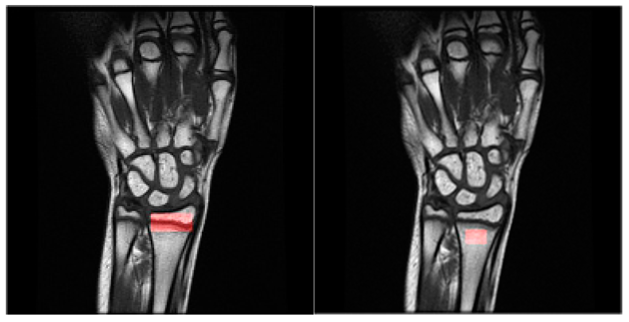
Most bone age assessment techniques implement X-ray-based imaging modalities that are invasive to some extent for patients. In this work, we would like to test whether other, non-invasive imaging techniques enable an accurate age estimation from acquired images that contain bone tissue. The aim of the present study was to explore whether the long bone textural analysis of the growth region on MRI images reflects changes in the age of the child and can possibly be applied for the determination of the bone age. To perform that examination, a dedicated database of MRI scans of adolescent hands was prepared. The descriptive region in the scan was marked manually, and then the textural features were extracted and the regression analysis was applied.

2. Materials and Methods

To verify whether it is possible to determine bone age from MRI images, a suitable dataset had to be prepared. The data acquisition is described in detail. The dataset gathered is briefly described. Next, the proposed textural features are presented, and details concerning the experiment quality measurements are given, followed by a description of experiment methodology.

2.1. Data Acquisition

This study was carried out according to the guidelines of good medical practice. The images were taken from a group of male volunteers, and the acquisition was approved by the Ethics Committee of Jagiellonian University (permission no. 1072.6120.16.2017) and complied with the Declaration of Helsinki. Written informed consent for participants was obtained from their legal guardians. The left hand of 30 healthy boys was examined by a 1.5 T system (GE Optima 360, Chicago, IL, USA) with a dedicated four-channel wrist coil. The acquisition was performed in a prone ‘superman’, e.g., with a hand erected in the overhead position.
Table 1 presents the parameters used to create T1-weighted and T2-weighted images. During the acquisition, 286 × 286 matrix size was used for the study. The scanning time of one sequence was in the range of 87–124 s. Radius growth plates were analyzed in coronal scans. Images were archived using the SIEMENS PACS (SYNGO, Siemens Healthineers, Erlangen, Germany). Anonymized studies were subsequently retrieved for image post-processing. The qMaZda software [54] was used for the computation of texture feature maps. Images with non-correctable motion artifacts were rejected. Small corrections of movement artifacts were performed with the use of pixel-by-pixel positioning of the overlaid images, and masks were developed that could compensate for the horizontal and vertical movements by a given number of pixels in case of minor movements.

2.2. Dataset Description

The dataset consists of images that show the bone structure of the non-dominant hand (left in all cases analyzed). The subject’s ages ranged from 9 to 17, with an average age of 12.43 and a median age of 12. The detailed distribution of age within the dataset is presented in Figure 1. There were accessible original DICOM (Digital Imaging and Communications in Medicine) images, and the visual information was stored in 12 bits. Furthermore, these images were normalized to the 0–255 range and stored as an 8-bit PNG image. In both cases, the image resolution is 512 × 512 pixels. Figure 2 presents an example of such a scan. In total, there are 55 images recorded with T1-weighted MRI and the same number of scans are collected with T2-weighted MRI. In image acquisition, we used a coronal plane of 3 mm thick, where a maximum of 10 layers were used in the plane with radius. From these data, up to three images per patient were considered usable considering their quality and visibility of the region of interest. In the case of the bone analysis, we used all 55 images; however, for radius growth region, only 30 images were used. The pixel spacing of the recorded data varies from 0.2539 to 0.3516 pixels, where the largest group of images was obtained for a 0.293 pixel spacing.

2.3. Data Analysis Methods and Methodology

The starting point of the data analysis was to select a descriptive region of interest (ROI), which well characterizes bone structure and allows for calculating the textural features, which become the mathematical description of the data. Since the pixel spacing of the data differs, we have decided to test two approaches. Firstly, a constant ROI size was selected in the MRI of the forearm. Second, the ROI size differed assuring the same metric units. These regions were applied to the DICOM and PNG versions of the data. Moreover, two regions with different medical meanings were considered: the bone and the growth region; please refer to Figure 2 for visualization.
For each region, the textural features were calculated using the qMaZda software. The software supports rich functionality, from which we have chosen several options. At the beginning, ±3σ normalization of the input region I(x,y) was applied. It is beneficial when the image histogram is close to the Gaussian, and it was also proved that better results are obtained for MR data. For an image, the mean μ and standard deviation σ of illuminance were calculated. Then, the image was scaled by recalculating minnorm = μ − 3σ and maxnorm = μ + 3σ, and finally, thresholded, according to Equations (1) and (2):
N x , y = I x , y min norm max norm     min norm
I n o r m x , y = 255 N x , y > 255 N ( x , y ) 0 N ( x , y ) 255 0 N x , y < 0
Then, for the region, the textural features were calculated. Starting from the first-order features that describe illumination distribution within the histogram, by 9 parameters: mean, variance, skewness, kurtosis, and percentiles 1, 10, 50, 90, and 99. The spatial relations between pixels were also exploited to derive features from the gray-level co-occurrence matrix (GLCM) [27], run-length matrix (RLM) [55], gradient matrix [27], first-order autoregressive model (AR) [56], Haar wavelet transform (HW) [57], Gabor transforms, and histogram of oriented gradients (HOG) [58]. There are 11 parameters calculated from the GLCM matrix in four spatial directions: horizontal, vertical, and two diagonals. This method is additionally parametrized with a distance between pixels treated as neighbors. In our research, this distance was set in a range from 1 to 5 pixels. Taking into account all those combinations (11 × 4 × 5), 220 features were obtained. From the RLM method, 20 additional parameters were calculated. This method gives five features, and they were calculated using the same four directions as in the GLCM method. There were five gradient matrices built with a high-pass filter using a 3 × 3 pixel mask. There were five features derived from the AR method. Their idea is based on the finding that brightness depends on the weighted sum of the neighboring pixels. The HW transform brings 16 parameters, which result from four down-sampled sub-images representing the energy of the data after conversion to the wavelet transform. In the case of the Gabor filter, the transformation was calculated in four directions (as for GLCM) using six Gaussian envelopes of the following sizes: 4, 6, 8, 12, 16, and 24. That gives 24 parameters. Finally, an eight-bin histogram of occurrences of gradient orientation in the image was calculated as a feature of the HOG method. After all, those transformations’ 307 features were obtained. The details on how to calculate each of these features are given in Appendix A.
Since the number of calculated features was large compared to the number of training samples, the reduction in feature space was necessary to remove redundancies and highly correlated data and improve the model’s possibility to derive patterns from the data. This was achieved by using principal component analysis (PCA). Finally, the bilayered perceptron neural network implemented in the Matlab Regression Learner toolbox was applied to perform the analysis. Since the datasets are small, the leave-one-out (LOO) cross-validation schema was used to validate the neural network. This means that the network was trained for all data samples except one. The remaining sample was used for validation. This process was repeated for all samples in the dataset, so that each sample was validated separately. In the LOO approach, the bias associated with the random selection of data for folds (as in the case of cross-validation) or with the selection of the test set (as in the case of train-test split) is reduced. Furthermore, the performance of the model can be assessed for each sample. The LOO method is recommended and is quite commonly used in the case of small datasets (from a dozen to several dozen samples) [59,60,61,62,63].
The quality regression model was evaluated by mean square error (MSE), root mean square error (RMSE), mean absolute error (MAE), and coefficient of determination (R2).

2.4. Experiment Setup

In the experiments performed, images of bone and growth regions have been analyzed. In the case of bones, all 55 images were used. However, for the growth region analysis, each patient was represented by only one image, which reduced the number of samples to 30. In this research, we have focused on the metric version of the annotation. Since the textural features depend strongly on the pixel relations, varying sizes of pixels might influence the outcomes, whereas when we had each time data with similar pixel spacing, this problem and its influence on results could be neglected. We performed a regression analysis regarding the patient’s full age. However, we noticed that the correlation improved when comparing texture features with the age given in months. Although that was an interesting finding, because of the small number of samples, it was abandoned for further investigation. The image preprocessing with the qMaZda software generated many texture features (307) to describe each sample. Using so many features can decrease regressor capabilities when most of them may not be correlated with the patient’s age. Therefore, a Spearman correlation between textural features and outcomes was calculated, which helped us choose 15 highly correlated, representative features. This procedure was applied to the training data separately for each model. Furthermore, as proven by previous research, these indicated the best textural features [64]. For this set of data, PCA was applied to derive the most discriminative parameters and remove any existing correlation between them. For bone and growth region analysis, the first 3 PCA eigenvectors were selected. The assumed number of PCA features used in regression analysis reflected the number of samples analyzed (55 in the case of bone image experiments and 30 when the growth region was evaluated). Experiments were performed for all four datasets: DICOM T1-weighted, DICOM T2-weighted, PNG T1-weighted, and PNG T2-weighted images. Furthermore, two tasks were evaluated: (1) finding the relation between the textural features of the bone region and the age of the patient; and (2) evaluating the dependence of the textural features in the growth region on the age of the patient.

3. Results

Table 2 and 
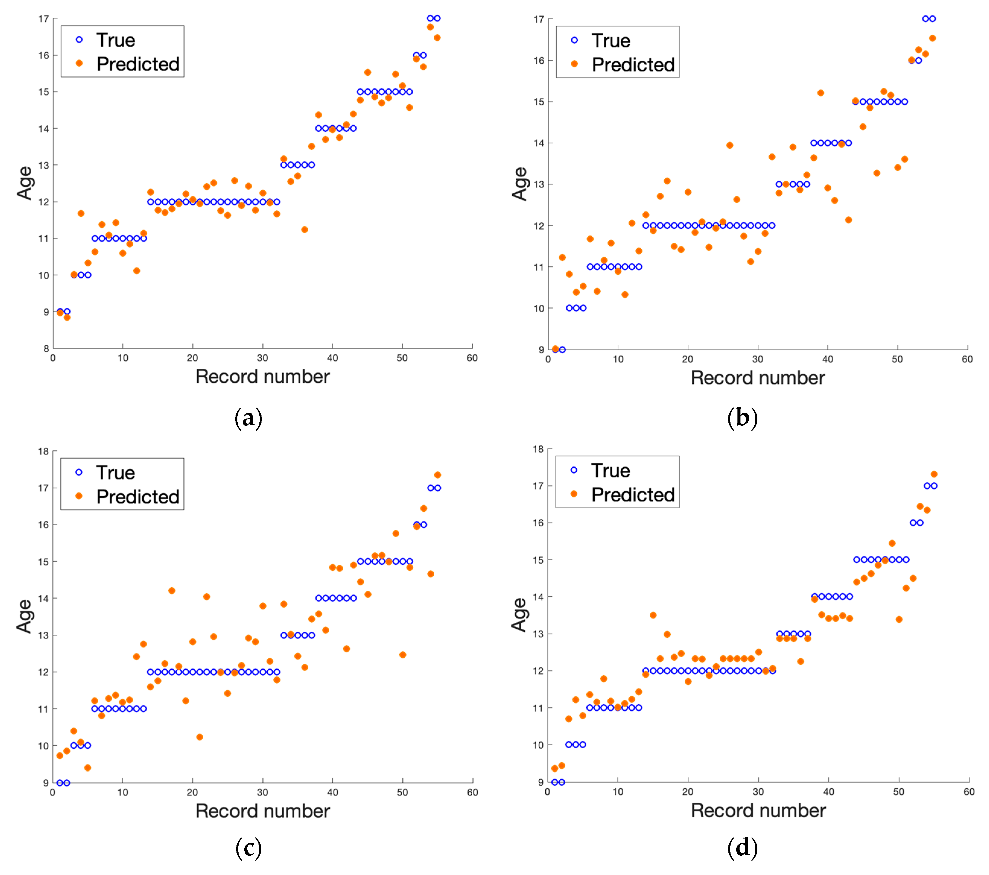
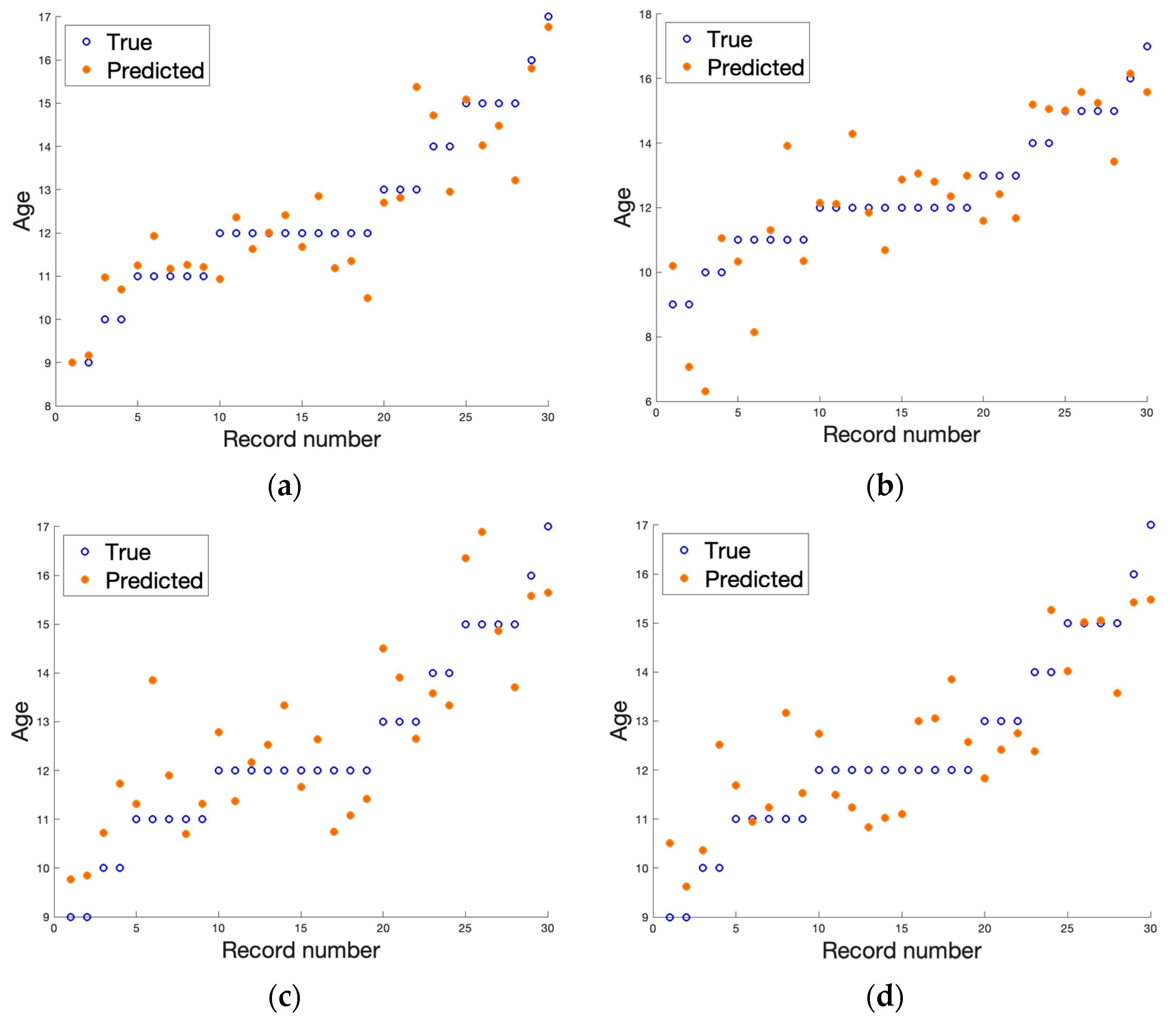
Table 3 collect the best results obtained after applying a two-layer neural network from the Matlab Regression Learner toolbox. The visualization of the results is depicted in Figure 3 and Figure 4. The results presented in Table 2 and Table 3 are the average values of the regression errors obtained for each of the samples. The plots summarize the results of all the LOO trials. From the results presented, we can see that the regression analysis in all cases allowed the prediction of the age of a patient based on the textural features analysis of the MRI data. The gathered results suggest that, considering the bone region, we achieved more stable results with fewer errors. However, due to the limited amount of data, these discrepancies between the analyzed regions could be due to decreasing the number of samples from 55 (for the bone) to 30 (for the growth region). The dispersion coefficient is very high, yet significantly better results were obtained when a T1-weighted image using the original 12-bit DICOM data was considered. We achieved the best score, which was R2 equal to 0.94 for the original 12-bit representation (DICOM) when the bone region was evaluated. In this scenario, second place was taken by the T2-weighted image with a reduced number of bits to eight (R2 equals 0.87). When analyzing the results obtained for the growth region (see Table 3), again, the T1-weighted image in 12-bit format returns the best outcomes, yet other results deteriorate significantly. This finding was also reflected in the other error metrics showing the smallest error in the case of DICOM T1-weighted datasets (see bold font in Table 2 and Table 3). The slight difference in the quality of age prediction by the chosen regressors was also noticeable in the plots presented in Figure 3 and Figure 4. Here, the predictions go through all observations in the case of analyzing textural features from bone DICOM T1-weighted images (see Figure 3a) and are very close to this line when the growth region DICOM T1-weighted images are considered (see Figure 4a). Since the true age was rounded to an integer value, the small discrepancies should not be surprising, as in reality, patients had a different number of months. As we noticed previously, the data reflected better when a shorter period was considered.

4. Discussion

Radiographic techniques are well-established methods that are used for the determination of bone age [12,13]. There are techniques that are based not only on the wrist estimation but also on other parts of the skeleton, including the clavicle [65], elbow [66], pelvis [67,68], humerus [69], or calcaneus [70,71]. Dental studies become a focus as body parts are used for age estimation [72,73,74].
Moreover, with the development of computer hardware, different techniques were proposed to obtain information from the image, allowing for the creation of efficient age evaluation systems, for example, Shorthand and BoneXpert to name a few [75,76]. There are many modern techniques that are based on shape extraction algorithms with comparative techniques, including those based on artificial intelligence [77,78,79,80]. However, many of these methods are still based on an X-ray analysis, where X-ray dose issues cannot be omitted.
Age determination based on a single radiograph is associated with low doses [81]. However, a cumulative dose in cases where multiple X-rays must be performed might not be acceptable. Ultrasonography, however, which is free from radiation and easy to use, is known as an operator-dependent method, which is a serious drawback of this otherwise useful technique [82].
MR was proposed as a method free of radiation exposure, but it is also repetitive, and in this regard, according to the results, it is stable. Table 4 provided a comparison of the MAE metric for our solution and other approaches working on X-ray data. As we can see, it outperformed other methods markedly. A certain drawback of MRIs is the time needed for the exam, which forces cooperation with young patients. Regarding the success of the MR examination, parental assistance is very important [24]. Child safety and comfort was assured in this study. That was very important as unintentional movement caused by inconvenient body alignment disturbs image creation. This is especially important in a proposed method where a small region of interest in the growth plate is used; therefore, a perfect image is key to the success of the proposed solution. Child cooperation is mandatory. However as described by Terada et al. [23] and Dvorak et al [22], short exam time was sufficient condition to ensure the creation of proper images. In our study, in contradiction to the protocol proposed by Dvorak et al. [22], Hojreh et al. [26], Stern et al. [83], and Quasim et al. [84], in addition to the T1-weighted spin echo and the gradient echo sequence (as applied in [23,24]), a T2-weighted spin echo was used. The choice of a T2-weighted sequence was dictated by the need to discriminate the number of watery progenitor cells because the amount of signals from these watery compounds was used as an indicator of the immaturity of the growth zone. The dependence of the growth zone composition on age with possible detection with the MR technique was described in experimental and clinical studies by Ecklund et al. [85], who described the dependence of the signal of the growth region composition. This agrees with histological studies proposed by Ballock et al. [86] and Breur et al. [87], who precisely described the basis of the known fact that the pattern of ongoing calcification of the growth region reflects maturation with age, which is at the core of the signal changes that are analyzed in our study as one of the discriminators of long bone maturation. In a study by Yun et al. [88], the dependence between the MR growth plate signal assessed in MR and skeletal maturation was not presented; however, the authors performed a study in the younger children group. One must remember that the proposed analysis of the growth plate is based on the narrow tissue element of progenitor cells, which is less than 3 mm and is a niche compared to the surrounding bone [89,90].
Despite the relatively low volume of the growth region in the composition of highly watery cells, it is highly detectable by high MR sequences, which in the image analysis, were reflected by a high correlation with histogram parameters (a sensitive indicator of brightness distribution but not necessarily structure) and supported by the presented regression analysis. This is logical because, in the zone of highly watery progenitor cells, the defined structure is very sparse, but the signal is strong. It can be observed that the younger the patient (with a wider growth region and more fluid), the brighter the signal. In older children, the amount of watery progenitor cells was reduced at the expense of the calcified bone rim, with a subsequent reduction in the influence of the bright area.
In a comparison of the T1-weighted and T2-weighted sequences, regression occurred more accurately for T1-weighted images than for T2-weighted signals, which is at least in part due to a high tissue contrast created between less hydrated trabeculae due to hydroxyapatite and therefore, low signal bone elements and high signal bone marrow [37,38]. The discriminative effect of the T2-weighted image due to the good differentiation between the unconverted bone marrow and the trabeculae can be partially spoiled by shift artifacts due to chemical composition, but also by the thickness of the trabeculae [91,92].
A slight influence on the results was observed regarding the type of encoding, the DICOM format was better with the T1-weighted sequence, which might be due to the overall contrast in the image where the T1-weighted sequence sensitive to water produces high signal differentiation in the image that is associated with a significant amount of blood morphotic elements in the immature marrow. This observation is consistent with clinical observations where sequences with a high TR time are used to differentiate lesions due to high visual contrast [93]. It is also worth mentioning that comparing different MRI sequences is problematic; however, there are works showing that the registration of two series of MRI data is possible to some extent [94].
Recently, new algorithms for automated bone marrow segmentation from MRI data have been developed [95,96]. We are going to implement such algorithms in our future research, especially when a large image database will be collected. The challenge will be to modify these algorithms in such a way as to select a specific ROI from the segmented, whole bone marrow. We know that radiomic features are prone to many problems. One of them is the low repeatability of texture features when multicenter studies are performed. On the other hand, such studies are essential to ensure the reliable validation of the developed machine learning models. It was shown in [97] that normalization applied to muscle tissue images acquired by different MR scanners improved the reproducibility of the calculated selected texture features. We will further investigate the influence of various ROI normalization schemes’ texture feature repeatability and reproducibility. Another factor that affects the calculation of bone marrow radiomic features is the variation of signal intensity between different scanners [98] as well as its dependence on signal blur phenomena. It is mostly caused by a chemical shift and magnetic susceptibility artifact, which belong to a class of tissue-specific artifacts. Other, less important might be also geometric artifacts that come from tissue tilt. Bone marrow analysis is always challenging and requires optimal image acquisition and compensation of acquisition artifacts.
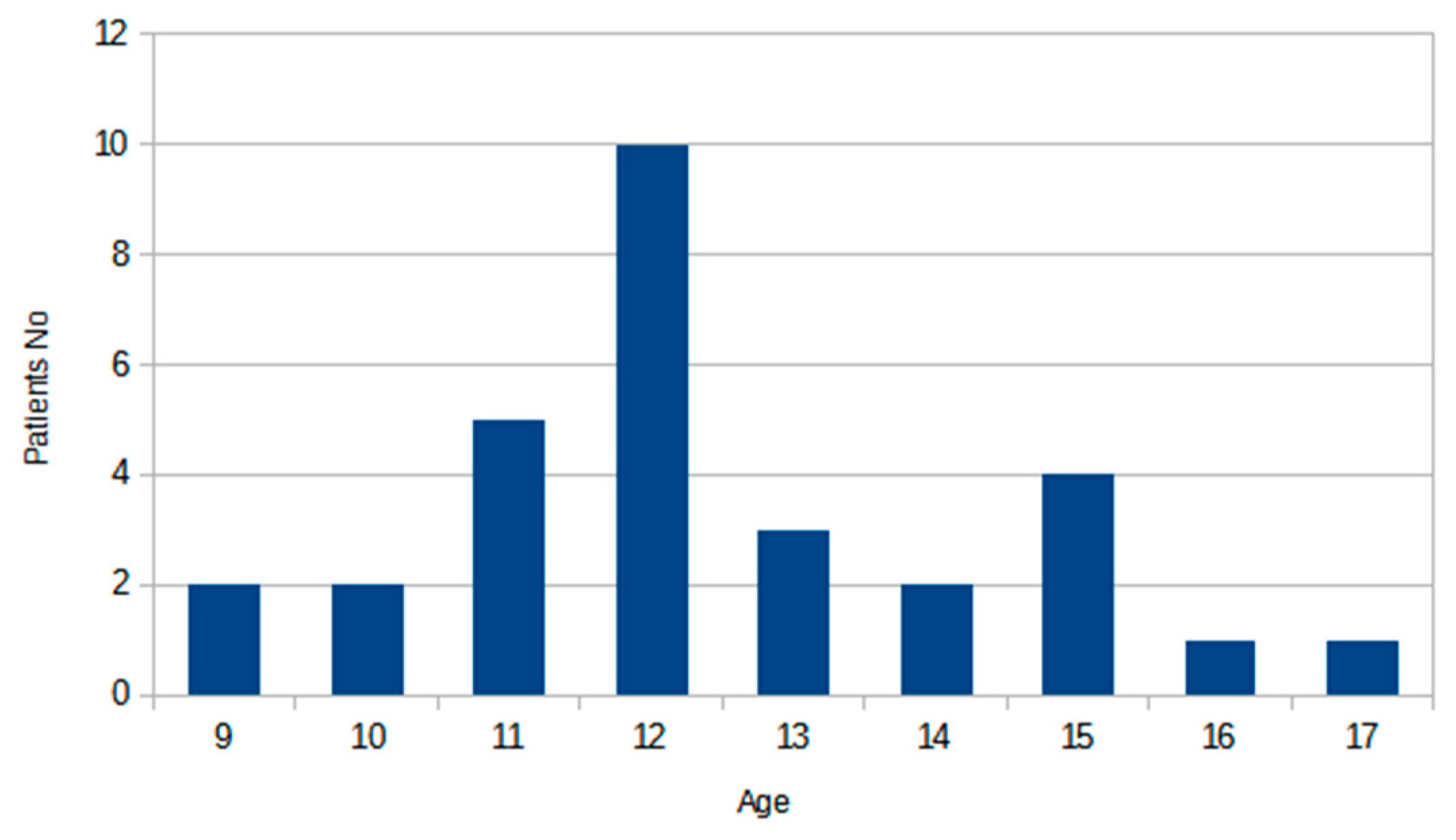
There are some limitations to this study. First, the image acquisition was relatively long. However, the scanning time was successfully overcome by the cooperative and motivated children. Since it was a pilot study and we only wanted to verify the hypothesis that it is possible to determine the bone age with high accuracy from the MRI images, a small group of patients was examined. For further studies, it should be extended. Finally, the error in the segmentation of the growth plate must be considered, given the small area of interest and the averaging effect due to the influence of the surrounding tissues.

5. Conclusions

This preliminary study presented the feasibility of implementing MRI bone scans in the bone age estimation protocols as a novel approach based on an analysis of the internal bone structure based on tissue texture. This is a different approach in comparison to shape and volume analyses based on X-ray techniques that are used today. To verify the hypothesis that it is possible to estimate the patient’s age based on an MRI hand scan, a database of non-dominant hands of 30 children was acquired. On those scans, the regions of interest were manually selected, distinguishing the bone and growth regions, both annotated with a constant pixel spacing. For these regions, textural features were calculated using the qMaZda software. To select the most representative data, a correlation analysis was performed followed by the PCA transform. Then, regression analysis was applied, which revealed a high correlation between the DICOM T1 images and the age of the patients (for the remaining types of analyzed data, the correlation was moderate). This is a significant finding, as it supports the claim that the use of the radiation-free technique can replace the current protocol based on X-ray scans. Moreover, we see that the magnetic resonance images convey complete information about bone structure and can be used interchangeably with X-ray images. The presented approach that implements machine learning on textures visualized in MRI scans is a novel solution toward the most complete analysis of bone age information, allowing for an accurate assessment of the biological age of the patient.

Author Contributions

Conceptualization, R.O. and A.P.; methodology, R.O., A.P., K.N. and M.S.; software, R.O., M.P., A.P. and M.S.; validation, R.O. and K.N.; formal analysis, R.O., M.P. and M.S.; investigation, R.O., K.N., M.P. and A.P.; resources, R.O., A.P. and M.S.; data curation, R.O., M.P., A.P. and M.S.; writing—original draft preparation, R.O., K.N. and M.S.; writing—review and editing, R.O., K.N., A.P. and M.S.; visualization, R.O., K.N., M.P. and A.P.; supervision, R.O., A.P. and M.S.; project administration, R.O., A.P. and M.S. All authors have read and agreed to the published version of the manuscript.

Funding

This research received no external funding.

Institutional Review Board Statement

The study was carried out in accordance with the Declaration of Helsinki and approved by the Institutional Review Board (or Ethics Committee) of Jagiellonian University (protocol code: 1072.6120.16.2017 and date of approval: 21 December 2017).

Informed Consent Statement

Patient consent was waived due to the retrospective nature of the research and access to the anonymized data.

Data Availability Statement

Data is unavailable due to privacy.

Acknowledgments

We thank Wiesław Guz for his assistance during the completion of the MR images.

Conflicts of Interest

The authors declare no conflict of interest.

Appendix A

Here, the following points provide detailed information about the definition of the texture feature parameters that were used in presented research.
1.
First-order features
First-order features are calculated for a gray-scale image using formulae presented in Table A1. Here, h stands for the normalized histogram function of occurrences at the G pixel level for image of width W and height H.
Table A1. Formulae to calculate first order features from the gray-scale image.
Feature NameFormulae
Mean μ = 1 W · H x = 0 W 1 y = 0 H 1 I x , y = i = 0 G 1 i · h ( i ) (A1)
Variance σ 2 = 1 W · H x = 0 W 1 y = 0 H 1 ( I x , y μ ) 2 = i = 0 G 1 ( i μ ) 2 · h ( i ) (A2)
Skewness σ 3 i = 0 G 1 ( i μ ) 3 · h ( i ) (A3)
Kurtosis σ 4 i = 0 G 1 ( i μ ) 4 · h i 3 (A4)
Percentile i = 0 G 1 h i p e r c e n t i l e (A5)
2.
Gray-level co-occurrence matrix [27]
Table A2 presents the features derived from the gray-level co-occurrence matrix p. This matrix saves the information of the number of existing co-occurrence of pixels of intensities indexing this cells within an image in cells. It is calculated separately in four directions (horizontal, vertical, and two diagonals). It is also possible to parametrize the distance d between pixels considered as adjoining in our research d = 1…5. The G stands for the pixel gray-level values.
Table A2. Formulae to calculate gray level co-occurrence matrix from the gray-scale image.
Feature NameFormulae
Contrast i = 0 G 1 j = 0 G 1 i j 2 p ( i , j ) (A6)
Correlation i = 0 G 1 j = 0 G 1 i j p i , j µ i µ j δ i δ j
where µi is average and δi is standard deviation for pi
(A7)
Homogeneity i = 0 G 1 j = 0 G 1 p ( i , j ) 1 + i j 2 (A8)
Entropy i = 0 G 1 j = 0 G 1 p i , j l o g 2 ( p i , j ) (A9)
Angular second moment i = 0 G 1 j = 0 G 1 p 2 i , j (A10)
Sum average m = 1 G m p s u m m (A11)
Sum variance m = 1 G m s u m a v g 2 p s u m m (A12)
Difference variance m = 1 G i µ d i f 2 p d i f m (A13)
Difference entropy m = 1 G p d i f m log p s u m m (A14)
Sum entropy m = 1 G p s u m m log p s u m m (A15)
Sum of squares i = 0 G 1 j = 0 G 1 i µ 2 p ( i , j ) (A16)
3.
Run-length matrix [55]
The run-length matrix p stores information about the length of pixel runs having the same pixel value. Thus, here, each matrix cell is indexed by the pixel gray-level value G, and the length L. The total number of recorded runs is denoted by nr. Features derived from the run-length matrix are given in Table A3.
Table A3. Formulae to calculate run-length matrix features from the gray-scale image.
Feature NameFormulae
Short run emphasis 1 n r i = 0 G 1 j = 1 L p ( i , j ) j 2 (A17)
Long run emphasis 1 n r i = 0 G 1 j = 1 L p ( i , j ) · j 2 (A18)
Gray-level non-uniformity 1 n r i = 0 G 1 j = 1 L p ( i , j ) (A19)
Run-length non-uniformity 1 n r j = 1 L i = 0 G 1 p ( i , j ) (A20)
Run percent n r W · H (A21)
4.
Gradient matrix [27]
The gradient magnitude for image region of interest I is calculated as follows:
Ɗ = I x , y + 1 I ( x , y 1 ) 2 + I x + 1 , y I ( x 1 , y ) 2
and within this region the mean, variance, skewness, and kurtosis are calculated (see formulas already presented for first-order features in Table A1) and additionally, the non-zeros parameter is computed as a ratio of |Ɗ| > 0 to all pixels in region of interest.
5.
First order autoregressive model [56]
The autoregressive model with four θ parameters is given with formulae:
I x , y = θ 1 I x 1 , y µ + θ 2 I x , y 1 µ + θ 3 I x 1 , y 1 µ + θ 4 I x + 1 , y 1 µ + µ + e x , y
where
µ = x , y R O I I x , y x , y R O I 1
and e stands for error.
6.
Haar wavelet transform [57]
A Haar discrete wavelet transform with its energies and frequencies is applied to four sub-band images returning the energy and three low-pass (L) and high-pass (H) filters in horizontal and vertical directions: HH, LH, and HL.
7.
Gabor transform
The Gabor transform locally decomposes the image and is calculated separately in four directions (horizontal, vertical, and both diagonals). The frequency components are computed by convolution with a kernel:
k x , y = e ( x 2 + y 2 ) 2 δ 2 c o s β + j s i n β where   β = ω x cos α + y sin α
where the parameters define the frequency ϖ, orientation α, and standard deviation of the Gaussian envelope δ. The average magnitude is calculated as follows:
M a g = x , y R O I k x , y x , y R O I 1
and the ROI’ is morphologically eroded.
8.
Histogram of oriented gradients [58]
Histogram of oriented gradients divides the image into 8 × 8 pixels cells, where the gradient’s magnitudes and directions are calculated. This information is coded into an 8-bin histogram, where the bins reflect the quantized gradient directions.

References

  1. Schmitt, A. Forensic Anthropology and Medicine: Complementary Sciences from Recovery to Cause of Death; Humana: Paramus, NJ, USA, 2006; pp. 212–219. [Google Scholar]
  2. Abdelbary, M.H.; Abdelkawi, M.M.; Nasr, M.A. Age determination by MR imaging of the wrist in Egyptian male foot ballplayers How far is it reliable? Egypt. J. Radiol. Nucl. Med. 2018, 49, 146–151. [Google Scholar] [CrossRef]
  3. Dekhne, M.S.; Kocher, I.D.; Hussain, Z.B.; Feroe, A.G.; Sankarankutty, S.; Williams, K.A.; Heyworth, B.E.; Milewski, M.D.; Kocher, M.S. Tibial tubercle apophyseal stage to determine skeletal age in pediatric patients undergoing ACL Reconstruction: A validation and reliability study. Orthop. J. Sports Med. 2021, 9, 23259671211036897. [Google Scholar] [CrossRef] [PubMed]
  4. Schmidt, S.; Koch, B.; Schulz, R.; Reisinger, W.; Schmeling, A. Studiesin use of the Greulich–Pyle skeletal age method to assess criminal liability. Legal Med. 2008, 10, 190–195. [Google Scholar] [CrossRef]
  5. Malina, R.M. Skeletal age and age verification in youth sport. Sports Med. 2011, 41, 925–947. [Google Scholar] [CrossRef] [PubMed]
  6. Schmeling, A.; Reisinger, W.; Geserick, G.; Olze, A. Age estimation of unaccompanied minors: Part I. General considerations. Forensic Sci. Int. 2006, 159, S61–S64. [Google Scholar] [CrossRef] [PubMed]
  7. Menjívar, C.; Perreira, K.M. Undocumented and unaccompanied: Children of migration in the European Union and the United States. J. Ethn. Migr. Stud. 2019, 45, 197–217. [Google Scholar] [CrossRef] [PubMed] [Green Version]
  8. Reinehr, T.; de Sousa, G.; Wabitsch, M. Relationships of IGF-I and androgens to skeletal maturation in obese children and adolescents. J. Pediatr. Endocrinol. Metab. 2006, 19, 1133–1140. [Google Scholar] [CrossRef] [PubMed]
  9. Phillip, M.; Moran, O.; Lazar, L. Growth without growth hormone. J. Pediatr. Endocrinol. Metab. 2002, 15, 1267–1272. [Google Scholar] [PubMed]
  10. Cox, L.A. The biology of bone maturation and ageing. Acta Paediatr. Suppl. 1997, 423, 107–108. [Google Scholar] [CrossRef]
  11. Kaplowitz, P.; Srinivasan, S.; He, J.; McCarter, R.; Hayeri, M.R.; Sze, R. Comparison of bone age readings by pediatric endocrinologists and pediatric radiologists using two bone age atlases. Pediatr. Radiol. 2010, 41, 690–693. [Google Scholar] [CrossRef]
  12. Greulich, W.W.; Pyle, S.I. Radiographic Atlas of Skeletal Development of the Hand and Wrist, 2nd ed.; Stanford University Press: Stanford, CA, USA, 1959. [Google Scholar]
  13. Tanner, J.M.; Whitehouse, R.H.; Healy, M. A New System for Estimating Skeletal Maturity from the Hand and Wrist with Standards Derived from a Study of 2600 Healthy British Children; Centre International de L’enfance: Paris, France, 1962. [Google Scholar]
  14. Alshamrani, K.; Messina, F.; Offiah, A.C. Is the Greulich and Pyle atlas applicable to all ethnicities? A systematic review and meta-analysis. Eur. Radiol. 2019, 29, 2910–2923. [Google Scholar] [PubMed] [Green Version]
  15. Alshamrani, K.; Offiah, A.C. Applicability of two commonly used bone age assessment methods to twenty-first century UK children. Diag. Interv. Radiol. 2020, 30, 504–513. [Google Scholar] [CrossRef] [Green Version]
  16. van Rijn, R.R.; Lequin, M.H.; Robben, S.G.; Hop, W.C.; van Kuijk, C. Is the Greulich and Pyle atlas still valid for Dutch Caucasian children today. Pediatr. Radiol. 2021, 31, 748–752. [Google Scholar] [CrossRef]
  17. Cantekin, K.; Celikoglu, M.; Miloglu, O.; Dane, A.; Erdem, A. Bone age assessment: The applicability of the Greulich-Pyle method in eastern Turkish children. J. Forensic Sci. 2012, 57, 679–682. [Google Scholar] [CrossRef] [PubMed]
  18. Dembetembe, K.A.; Morris, A.G. Is Greulich-Pyle age estimation applicable for determining maturation in male Africans. South Afr. Sci. Suid-Afrik. Wet. 2012, 108, 1–6. [Google Scholar] [CrossRef]
  19. Mentzel, H.-J.; Vilser, C.; Eulenstein, M.; Schwartz, T.; Vogt, S.; Böttcher, J.; Yaniv, I.; Tsoref, L.; Kauf, E.; Kaiser, W.A. Assessment of skeletal age at the wrist in children with a new ultrasound device. Pediatr. Radiol. 2005, 35, 429–433. [Google Scholar] [CrossRef] [PubMed]
  20. Khan, K.M.; Miller, B.S.; Hoggard, E.; Somani, A.; Sarafoglou, K. Application of ultrasound for bone age estimation in clinical practice. J. Pediatr. 2009, 154, 243–247. [Google Scholar] [CrossRef]
  21. Bilgili, Y.; Hizel, S.; Kara, S.A.; Sanli, C.; Erdal, H.H.; Altinok, D. Accuracy of skeletal age assessment in children from birth to 6 years of age with the ultrasonographic version of the Greulich-Pyle atlas. J. Ultrasound Med. 2003, 22, 683–690. [Google Scholar] [CrossRef]
  22. Dvorak, J.; George, J.; Junge, A.; Hodler, J. Age determination by magnetic resonance imaging of the wrist in adolescent male football players. Br. J. Sports Med. 2007, 41, 45–52. [Google Scholar] [CrossRef] [Green Version]
  23. Terada, Y.; Kono, S.; Tamada, D.; Uchiumi, T.; Kose, K.; Miyagi, R.; Yamabe, E.; Yoshioka, H. Skeletal age assessment in children using an open compact MRI system. Magn. Reson. Med. 2013, 69, 1697–1702. [Google Scholar] [CrossRef]
  24. Terada, Y.; Kono, S.; Uchiumi, T.; Kose, K.; Miyagi, R.; Yamabe, E.; Fujinaga, Y.; Yoshioka, H. Improved reliability in skeletal age assessment using a pediatric hand MR scanner with a 0. 3T permanent magnet. Magn. Reson. Med. Sci. 2014, 13, 215–219. [Google Scholar] [CrossRef] [PubMed] [Green Version]
  25. Tomei, E.; Sartori, A.; Nissman, D.; Al Ansari, N.; Battisti, S.; Rubini, A.; Stagnitti, A.; Martino, M.; Marini, M.; Barbato, E.; et al. Value of MRI of the hand and the wrist in evaluation of bone age: Preliminary results. J. Magn. Reson. Imaging 2014, 39, 1198–1205. [Google Scholar] [CrossRef] [PubMed]
  26. Hojreh, A.; Gamper, J.; Schmook, M.T.; Weber, M.; Prayer, D.; Herold, C.J.; Noebauer-Huhmann, I.M. Hand MRI and the Greulich-Pyle atlas in skeletal age estimation in adolescents. Skelet. Radiol. 2018, 47, 963–971. [Google Scholar] [CrossRef] [PubMed] [Green Version]
  27. Haralick, R.M. Statistical and structural approaches to texture. Proc. IEEE 1979, 67, 786–804. [Google Scholar] [CrossRef]
  28. Haralick, R.M.; Shanmugam, K.; Dinstein, I. Textural Features for Image Classification. IEEE Trans. Syst. Man. Cybern. 1973, 3, 610–621. [Google Scholar] [CrossRef] [Green Version]
  29. Kociołek, M.; Strzelecki, M.; Klepaczko, A. Functional kidney analysis based on textured DCE-MRI images, In Advances in Intelligent Systems and Computing; Piętka, E., Badura, P., Kawa, J., Wieclawek, W., Eds.; Springer Verlag: Berlin/Heidelberg, Germany, 2019; pp. 38–49. [Google Scholar]
  30. Szczypiński, P.M.; Strzelecki, M.; Materka, A.; Klepaczko, A. MaZda—The software package for textural analysis of biomedical images. Adv. Intell. Soft Comput. 2009, 65, 73–84. [Google Scholar]
  31. Materka, A. Texture analysis methodologies for magnetic resonance imaging. Dialogues Clin. Neurosci. 2022, 6, 243–250. [Google Scholar] [CrossRef]
  32. Chrzanowski, L.; Drozdz, J.; Strzelecki, M.; Krzeminska-Pakula, M.; Jedrzejewski, K.; Kasprzak, J. Application of neural networks for the analysis of histological and ultrasonic aortic wall appearance—An in-vitro tissue characterization study. Ultrasound Med. Biol. 2008, 34, 103–113. [Google Scholar] [CrossRef]
  33. Obuchowicz, R.; Kruszyńska, J.; Strzelecki, M. Classifying median nerves in carpal tunnel syndrome: Ultrasound image analysis. Biocybern. Biomed. Eng. 2021, 41, 335–351. [Google Scholar] [CrossRef]
  34. Hochberg, Z. Clinical physiology and pathology of the growth plate. Best Pract. Res. Clin. Endocrinol. Metab. 2002, 16, 399–419. [Google Scholar] [CrossRef]
  35. Jaramillo, D.; Laor, T.; Zaleske, D.J. Indirect trauma to the growth plate: Results of MR imaging after epiphyseal and metaphyseal injury in rabbits. Radiology 1993, 187, 171–178. [Google Scholar] [CrossRef] [PubMed]
  36. Wilsman, N.J.; Farnum, C.E.; Green, E.M.; Lieferman, E.M.; Clayton, M.K. Cell cycle analysis of proliferative zone chondrocytes in growth plates elongating at different rates. J. Orthop. Res. 1996, 14, 562–572. [Google Scholar] [CrossRef] [PubMed]
  37. Burdiles, A.; Babyn, P.S. Pediatric bone marrow MR imaging. Magn. Reson. Imaging Clin. N Am. 2009, 17, 391–409. [Google Scholar] [CrossRef]
  38. Chan, B.Y.; Gill, K.G.; Rebsamen, S.L.; Nguyen, J.C. MR Imaging of Pediatric Bone Marrow. Radiographics 2016, 36, 1911–1930. [Google Scholar] [CrossRef] [PubMed] [Green Version]
  39. Iglovikov, V.I.; Rakhlin, A.; Kalinin, A.A.; Shvets, A.A. Pediatric bone age assessment using deep convolutional neural networks. In Deep Learning in Medical Image Analysis and Multimodal Learning for Clinical Decision Support; Springer: Cham, Switzerland, 2018; pp. 300–308. [Google Scholar]
  40. Salim, I.; Hamza, A.B. Ridge regression neural network for pediatric bone age assessment. Multimed. Tools Appl. 2021, 80, 30461–30478. [Google Scholar] [CrossRef]
  41. Marouf, M.; Siddiqi, R.; Bashir, F.; Vohra, B. Automated hand X-ray based gender classification and bone age assessment using convolutional neural network. In Proceedings of the 2020 3rd International Conference on Computing, Mathematics and Engineering Technologies (iCoMET), Sukkur, Pakistan, 29–30 January 2020; pp. 1–5. [Google Scholar]
  42. Liu, B.; Zhang, Y.; Chu, M.; Bai, X.; Zhou, F. Bone age assessment based on rank-monotonicity enhanced ranking CNN. IEEE Access 2019, 7, 120976–120983. [Google Scholar] [CrossRef]
  43. Zulkifley, M.A.; Mohamed, N.A.; Abdani, S.R.; Kamari, N.A.M.; Moubark, A.M.; Ibrahim, A.A. Intelligent bone age assessment: An automated system to detect a bone growth problem using convolutional neural networks with attention mechanism. Diagnostics 2021, 11, 765. [Google Scholar] [CrossRef] [PubMed]
  44. Lee, H.; Tajmir, S.; Lee, J.; Zissen, M.; Yeshiwas, B.A.; Alkasab, T.K.; Choy, G.; Do, S. Fully automated deep learning system for bone age assessment. J. Digit. Imaging 2017, 30, 427–441. [Google Scholar] [CrossRef] [Green Version]
  45. Castillo, J.; Tong, Y.; Zhao, J.; Zhu, F. RSNA Bone-Age Detection Using Transfer Learning and Attention Mapping. In ECE228 and SIO209 Machine Learning for Physical Applications; 2018; pp. 1–5. Available online: http://noiselab.ucsd.edu/ECE228_2018/Reports/Report6.pdf (accessed on 1 February 2020).
  46. Karargyris, A.; Kashyap, S.; Wu, J.T.; Sharma, A.; Moradi, M.; Syeda-Mahmood, T. Age prediction using a large chest X-ray dataset. In Proceedings of the Medical Imaging 2019: Computer-Aided Diagnosis, San Diego, CA, USA, 16–21 February 2019; p. 10950. [Google Scholar]
  47. Nguyen, H.; Soohyung, K. Automatic whole-body bone age assessment using deep hierarchical features. arXiv 2019, arXiv:1901.10237. [Google Scholar]
  48. Janczyk, K.; Rumiński, J.; Neumann, T.; Głowacka, N.; Wiśniewski, P. Age prediction from low resolution, dual-energy X-ray images using convolutional neural networks. Appl. Sci. 2022, 12, 6608. [Google Scholar] [CrossRef]
  49. Castillo, R.F.; Ruiz, M.D.C.L. Assessment of age and sex by means of DXA bone densitometry: Application in forensic anthropology. Forensic Sci. Int. 2011, 209, 53–58. [Google Scholar] [CrossRef] [PubMed]
  50. Navega, D.; Coelho, J.D.O.; Cunha, E.; Curate, F. DXAGE: A new method for age at death estimation based on femoral bone mineral density and artificial neural networks. J. Forensic Sci. 2017, 63, 497–503. [Google Scholar] [CrossRef] [PubMed]
  51. Pietka, B.E.; Pośpiech, S.; Gertych, A.; Cao, F.; Huang, H.K.; Gilsanz, V. Computer automated approach to the extraction of epiphyseal regions in hand radiographs. J Digit Imaging. 2001, 14, 165–172. [Google Scholar]
  52. Pietka, E.; Gertych, A.; Pospiech-Kurkowska, S.; Cao, F.; Huang, H.K.; Gilzanz, V. Computer assisted bone age assessment: Graphical user interface for image processing and comparison. J. Digit. Imaging 2004, 17, 175–188. [Google Scholar] [CrossRef] [PubMed] [Green Version]
  53. Gertych, A.; Piętka, E.; Liu, B.J. Segmentation of regions of interest and post-segmentation edge location improvement in computer-aided bone age assessment. Pattern Anal. Appl. 2007, 10, 115. [Google Scholar] [CrossRef]
  54. Szczypinski, P.M.; Klepaczko, A.; Kociolek, M. QMaZda—Software tools for image analysis and pattern recognition. In Proceedings of the 2017 Signal Processing: Algorithms, Architectures, Arrangements, and Applications (SPA), Poznan, Poland, 20–22 September 2017; pp. 217–221. [Google Scholar]
  55. Galloway, M.M. Texture analysis using grey level run lengths. Comput. Graph. Image Process. 1975, 4, 172–179. [Google Scholar] [CrossRef]
  56. Kashyap, R.; Chellappa, R. Estimation and choice of neighbors in spatial-interaction models of images. IEEE Trans. Inf. Theory 1983, 29, 60–72. [Google Scholar] [CrossRef]
  57. Porter, R.; Canagarajah, N. Rotation invariant texture classification schemes using GMRFs and wavelets. In Proceedings of the Proceedings IWISP’96, Manchester, UK, 4–7 November 1996; pp. 183–186. [Google Scholar]
  58. Pierzchała, M.; Obuchowicz, R.; Guz, W.; Piórkowski, A. Correlation of the results of textural analysis of wrist MRI images with age in boys aged 9–17. Bio-Algorithms Med-Syst. 2021, 17, eA18–eA19. [Google Scholar]
  59. Hu, J.; Wang, Y.; Guo, D.; Qu, Z.; Sui, C.h.; He, G.; Wang, S.; Chen, X.; Wang, C.h.; Liu, X. Diagnostic performance of magnetic resonance imaging–based machine learning in Alzheimer’s disease detection: A meta-analysis. Neuroradiology 2023, 65, 513–527. [Google Scholar] [CrossRef]
  60. Snider, E.J.; Hernandez-Torres, S.I.; Hennessey, R. Using ultrasound image augmentation and ensemble predictions to prevent machine-learning model overfitting. Diagnostics 2023, 13, 417. [Google Scholar] [CrossRef]
  61. Shao, Y.; Hashemi, H.S.; Gordon, P.; Warren, L.; Wang, J.; Rohling, R.; Salcudean, S. Breast cancer detection using multimodal time series features from ultrasound shear wave absolute vibro-elastography. IEEE J. Biomed. Health Inform. 2022, 26, 704–714. [Google Scholar] [CrossRef] [PubMed]
  62. d’Este, S.H.; Nielsen, M.B.; Hansen, A.E. Visualizing glioma infiltration by the combination of multimodality imaging and artificial Intelligence, a systematic review of the literature. Diagnostics 2021, 11, 592. [Google Scholar] [CrossRef] [PubMed]
  63. Hoar, D.; Lee, P.Q.; Guida, A.; Patterson, S.; Bowen, C.V.; Merrimen, J.; Wang, C.; Rendon, R.; Beyea, S.D.; Clarke, S.E. Combined transfer learning and test-time augmentation improves convolutional neural network-based semantic segmentation of prostate cancer from multi-parametric MR images. Comput. Methods Programs Biomed. 2021, 210, 106375. [Google Scholar] [CrossRef] [PubMed]
  64. Dalal, N.; Triggs, B. Histograms of oriented gradients for human detection. In Proceedings of the 2005 IEEE Computer Society Conference on Computer Vision and Pattern Recognition (CVPR’05), San Diego, CA, USA, 20–26 June 2005; Volume 1, pp. 886–893. [Google Scholar] [CrossRef] [Green Version]
  65. Kreitner, K.F.; Schweden, F.J.; Riepert, T.; Nafe, B.; Thelen, M. Bone age determination based on the study of the medial extremity of the clavicle. Eur. Radiol. 1998, 8, 1116–1122. [Google Scholar] [CrossRef]
  66. Charles, Y.P.; Dimeglio, A.; Canavese, F.; Daures, J.-P. Skeletal age assessment from the olecranon for idiopathic scoliosis at Risser grade 0. J. Bone Joint Surg. Am. 2007, 89, 2737–2744. [Google Scholar] [CrossRef] [PubMed] [Green Version]
  67. Risser, J.C. The Iliac apophysis; an invaluable sign in the management of scoliosis. Clin. Orthop. 1958, 11, 111–119. [Google Scholar] [CrossRef] [Green Version]
  68. Little, D.G.; Sussman, M.D. The Risser sign: A critical analysis. J. Pediatr. Orthop. 1994, 14, 569–575. [Google Scholar] [CrossRef]
  69. Li, D.T.; Cui, J.J.; DeVries, S.; Nicholson, A.D.; Li, E.; Petit, L.; Kahan, J.B.; Sanders, J.O.; Liu, R.W.; Cooperman, D.R.; et al. Humeral head ossification predicts peak height velocity timing and percentage of growth remaining in children. J. Pediatr. Orthop. 2018, 38, E546–E550. [Google Scholar] [CrossRef] [PubMed]
  70. Nicholson, A.D.; Liu, R.W.; Sanders, J.O.; Cooperman, D.R. Relationship of calcaneal and iliac apophyseal ossification to peak height velocity timing in children. J. Bone Joint Surg. Am. 2015, 97, 147–154. [Google Scholar] [CrossRef]
  71. Li, S.Q.; Nicholson, A.D.; Cooperman, D.R.; Liu, R.W. Applicability of the calcaneal apophysis ossification staging system to the modern pediatric population. J. Pediatr. Orthop. 2019, 39, 46–50. [Google Scholar] [CrossRef]
  72. Demirjian, A.; Goldstein, H.; Tanner, J.M. A new system of dental age assessment. Hum. Biol. 1973, 45, 211–227. [Google Scholar] [PubMed]
  73. Sehrawat, J.S.; Singh, M. Willems method of dental age estimation in children: A systematic review and meta-analysis. J. Forensic Leg. Med. 2017, 52, 122–129. [Google Scholar] [CrossRef] [PubMed]
  74. Malik, P.; Saha, R.; Agarwal, A. Applicability of Demirjian’s method of age assessment in a North Indian female population. Eur. J. Paediatr. Dent. 2012, 13, 133–135. [Google Scholar]
  75. Heyworth, B.E.; Osei, D.A.; Fabricant, P.D.; Schneider, R.; Doyle, S.h.M.; Green, D.W.; Widmann, R.F.; Lyman, S.; Burke, S.W.; Scher, D.M. The shorthand bone age assessment: A simpler alternative to current methods. J. Pediatr. Orthop. 2013, 33, 569–574. [Google Scholar] [CrossRef]
  76. Thodberg, H.H.; Kreiborg, S.; Juul, A.; Pedersen, K.D. The BoneXpert method for automated determination of skeletal maturity. IEEE Trans. Med. Imaging 2009, 28, 52–66. [Google Scholar] [CrossRef] [PubMed]
  77. Wang, F.; Gu, X.; Chen, S.; Liu, Y.; Shen, Q.; Pan, H.; Shi, L.; Jin, Z. Artificial intelligence system can achieve comparable results to experts for bone age assessment of Chinese children with abnormal growth and development. PeerJ 2020, 8, e8854. [Google Scholar] [CrossRef]
  78. Liu, Y.; Zhang, C.; Cheng, J.; Chen, X.; Wang, Z.J. A multi-scale data fusion framework for bone age assessment with convolutional neural networks. Comput. Biol. Med. 2019, 108, 161–173. [Google Scholar] [CrossRef] [PubMed]
  79. Ren, X.; Li, T.; Yang, X.; Wang, S.; Ahmad, S.; Xiang, L.; Stone, S.R.; Li, L.; Zhan, Y.; Shen, D.; et al. Regression convolutional neural network for automated pediatric bone age assessment from hand radiograph. IEEE J. Biomed. Health Inform. 2019, 23, 2030–2038. [Google Scholar] [CrossRef]
  80. Tong, C.; Liang, B.; Li, J.; Zheng, Z. A Deep Automated Skeletal Bone Age Assessment Model with Heterogeneous Features Learning. J. Med. Syst. 2018, 42, 249. [Google Scholar] [CrossRef]
  81. Mettler, F.A.; Huda, W.; Yoshizumi, T.T.; Mahesh, M. Effective doses in radiology and diagnostic nuclear medicine: A catalog 1. Radiology 2008, 248, 254–263. [Google Scholar] [CrossRef]
  82. Xu, H.; Shao, H.; Wang, L.; Jin, J.; Wang, J. A Methodological comparison between ultrasound and X-ray evaluations of bone age. J. Sports Sci. 2008, 6, 27. [Google Scholar]
  83. Stern, D.; Ebner, T.; Bischof, H.; Grassegger, S.; Ehammer, T.; Urschler, M. Fully automatic bone age estimation from left hand MR images. In Medical Image Computing and Computer-Assisted Intervention—MICCAI 2014; Golland, P., Hata, N., Barillot, C., Hornegger, J., Howe, R., Eds.; Lecture Notes in Computer Science; Springer: Berlin/Heidelberg, Germany, 2014; Volume 8674. [Google Scholar]
  84. Qasim, M.S.h.; Abdullateef, A.; Mohammed, A.l.-H.; Najah, R.R. Magnetic resonance imaging of the left wrist: Assessment of the bone age in a sample of healthy Iraqi adolescent males. J. Fac. Med. 2015, 57, 22–26. [Google Scholar]
  85. Ecklund, K.; Jaramillo, D. Patterns of premature physeal arrest: MR imaging of 111 children. AJR Am. J. Roentgenol. 2002, 178, 967–972. [Google Scholar] [CrossRef] [PubMed]
  86. Ballock, R.T.; O'Keefe, R.J. The biology of the growth plate. J. Bone Joint Surg. Am. 2003, 85, 715–726. [Google Scholar] [CrossRef]
  87. Breur, G.J.; van Enkevort, B.A.; Farnum, C.E.; Wilsman, N.J. Linear relationship between the volume of hypertrophic chondrocytes and the rate of longitudinal bone growth in growth plates. J. Orthop. Res. 1991, 9, 348–359. [Google Scholar] [CrossRef]
  88. Yun, H.H.; Kim, H.J.; Jeong, M.S.; Choi, Y.S.; Seo, J.Y. Changes of the growth plate in children: 3-dimensional magnetic resonance imaging analysis. Korean. J. Pediatr. 2018, 61, 226–230. [Google Scholar] [CrossRef]
  89. Craig, J.G.; Cody, D.D.; van Holsbeeck, M. The distal femoral and proximal tibial growth plates: MR imaging, three-dimensional modeling and estimation of area and volume. Skelet. Radiol. 2004, 33, 337–344. [Google Scholar] [CrossRef] [PubMed]
  90. Stokes, I.A. Growth plate mechanics and mechanobiology. A survey of present understanding. J. Biomech. 2009, 42, 1793–1803. [Google Scholar]
  91. Mitchell, D.G.; Kim, I.; Chang, T.S.; Vinitski, S.; Consigny, P.M.; Saponaro, S.A.; Ehrlich, S.M.; Rifkin, M.D.; Rubin, R. Fatty liver: Chemical shift phase-difference and suppression magnetic resonance imaging techniques in animals, phantoms, and humans. Invest. Radiol. 1991, 26, 1041–1052. [Google Scholar] [CrossRef]
  92. Bley, T.A.; Wieben, O.; François, C.J.; Brittain, J.H.; Reeder, S.B. Fat and water magnetic resonance imaging. J. Magn. Reson. Imaging 2010, 31, 4–18. [Google Scholar] [CrossRef]
  93. Moon, W.J.; Lee, M.H.; Chung, E.C. Diffusion-weighted imaging with sensitivity encoding (SENSE) for detecting cranial bone marrow metastases: Comparison with T1-weighted images. Korean J. Radiol. 2007, 8, 185–191. [Google Scholar] [CrossRef] [Green Version]
  94. Bzowski, P.; Borys, D.; Guz, W.; Obuchowicz, R.; Piórkowski, A. Evaluation of the MRI Images Matching Using Normalized Mutual Information Method and Preprocessing Techniques. Adv. Intell. Syst. Comput. 2020, 1062, 92–100. [Google Scholar] [CrossRef]
  95. Wennmann, M.; Klein, A.; Bauer, F.; Chmelik, J.; Grözinger, M.; Uhlenbrock, C.; Lochner, J.; Nonnenmacher, T.; Rotkopf, L.T.; Sauer, S.; et al. Combining deep learning and radiomics for automated, objective, comprehensive bone marrow characterization from whole-body MRI. A multicentric feasibility study. Invest. Radiol. 2022, 57, 752–763. [Google Scholar] [CrossRef] [PubMed]
  96. Wennmann, M.; Neher, P.; Stanczyk, N.; Kahl, K.C.; Kächele, J.; Weru, V.; Hielscher, T.; Grözinger, M.; Chmelik, J.; Zhang, K.S.; et al. Deep learning for automatic bone marrow apparent diffusion coefficient measurements from whole-body magnetic resonance imaging in patients with multiple myeloma: A retrospective multicenter study. Invest. Radiol. 2023, 58, 273–282. [Google Scholar] [CrossRef] [PubMed]
  97. Wennmann, M.; Bauer, F.; Klein, A.; Chmelik, J.; Grözinger, M.; Rotkopf, L.T.; Neher, P.; Gnirs, R.; Kurz, F.T.; Nonnenmacher, T.; et al. In vivo repeatability and multiscanner reproducibility of MRI radiomics features in patients with monoclonal plasma cell disorders: A prospective bi-institutional study. Invest Radiol. 2023, 58, 253–264. [Google Scholar] [CrossRef] [PubMed]
  98. Wennmann, M.; Thierjung, H.; Bauer, F.; Weru, V.; Hielscher, T.; Grözinger, M.; Gnirs, R.; Sauer, S.; Goldschmidt, H.; Weinhold, N.; et al. Repeatability and Reproducibility of ADC Measurements and MRI Signal Intensity Measurements of Bone Marrow in Monoclonal Plasma Cell Disorders: A Prospective Bi-institutional Multiscanner.; Multiprotocol Study. Invest. Radiol. 2022, 57, 272–281. [Google Scholar] [CrossRef]
Figure 1. Distribution of the age of the patient within the dataset.
Jcm 12 02762 g001
Figure 2. Exemplary magnetic resonance imaging. The red rectangle shows the growth region in the image on the right and bone region on the left scan.
Jcm 12 02762 g002
Figure 3. The result of regression algorithms for all cases examined for data describing bone images (metric). The real age is presented by blue circles and estimated age with a regression algorithm is depicted by orange dots. The samples are ordered on the y axis with increasing age. (a) DICOM T1-weighted, (b) DICOM T2-weighted, (c) PNG T1-weighted, and (d) PNG T2-weighted.
Jcm 12 02762 g003
Figure 4. The result of regression algorithms for all examined cases for data describing growth region images (metric). The real age is given as a blue circle and age estimated with a regression algorithm is depicted as orange dot. The samples are ordered on the y axis with increasing age. (a) DICOM T1-weighted, (b) DICOM T2-weighted, (c) PNG T1-weighted, and (d) PNG T2-weighted.
Jcm 12 02762 g004
Table 1. Parameters used for acquisition of T1- and T2-weighted images.
ParameterT1-WeightedT2-Weighted
Slice thickness3 mm3 mm
Repetition Time435 ms2749 ms
Echo Time16 ms106 ms
Number of averages22
Spacing3.5 mm3.5 mm
Echo train length2323
Bandwidth81 MHz97 MHz
Table 2. Quantitative regression parameters for different types of data and bone images (metric). Results for 3 features derived from 15 by applying principal component analysis.
DataR2 RMSEMSEMAE
DICOM T1-weighted0.93830.45840.21010.3300
DICOM T2-weighted0.75100.83650.69970.6229
PNG T1-weighted0.72830.93440.87320.6922
PNG T2-weighted0.87110.57310.32840.4429
Table 3. Quantitative regression parameters for different types of data and growth region images (metric). Results for 3 features derived from 15 by applying principal component analysis.
DataR2 RMSEMSEMAE
DICOM T1-weighted0.80410.81940.67140.6142
DICOM T2-weighted0.66211.41041.98921.0969
PNG T1-weighted0.67431.05501.11300.8740
PNG T2-weighted0.52161.10581.22280.9228
Table 4. Results of performance of the presented method and other solutions for the estimation of bone age based on hand.
ReferencesMAE (Months)
Liu et al. [42]6.01
Iglovikov et al. [39]6.10
Salim and Hamza [40]6.38
Zulkifley et al. [43]7.70
MAE (years)
Nguyen et al. [47]4.856
Our method0.330 (T1 DICOM), 0.692 (T1 PNG)
Disclaimer/Publisher’s Note: The statements, opinions and data contained in all publications are solely those of the individual author(s) and contributor(s) and not of MDPI and/or the editor(s). MDPI and/or the editor(s) disclaim responsibility for any injury to people or property resulting from any ideas, methods, instructions or products referred to in the content.

