
Investigating the Dialysis Treatment Using Hollow Fiber Membrane: A New Approach by CFD

 , , , and
Abstract
:1. Introduction
2. Methodology
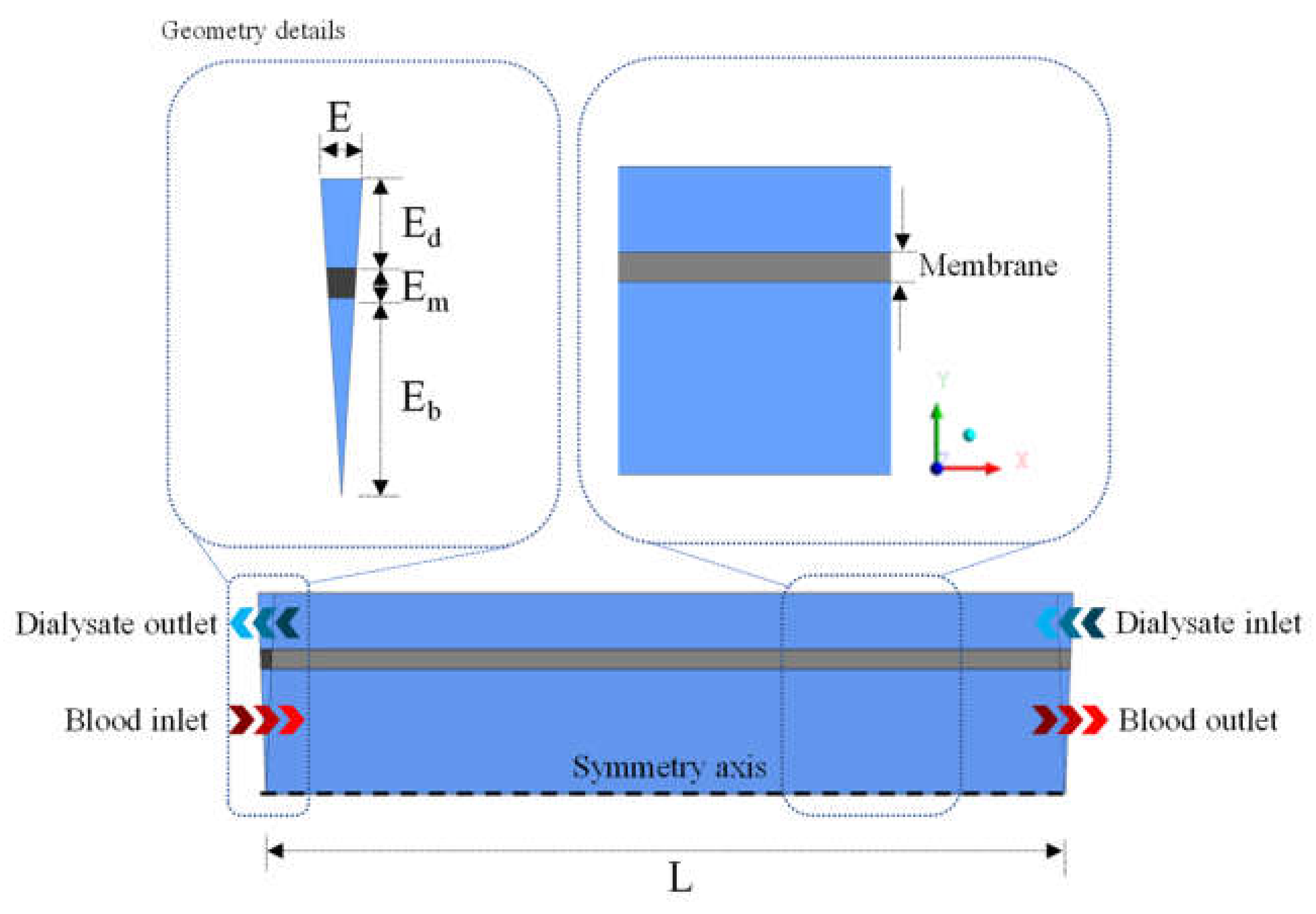
2.1. Problem Description
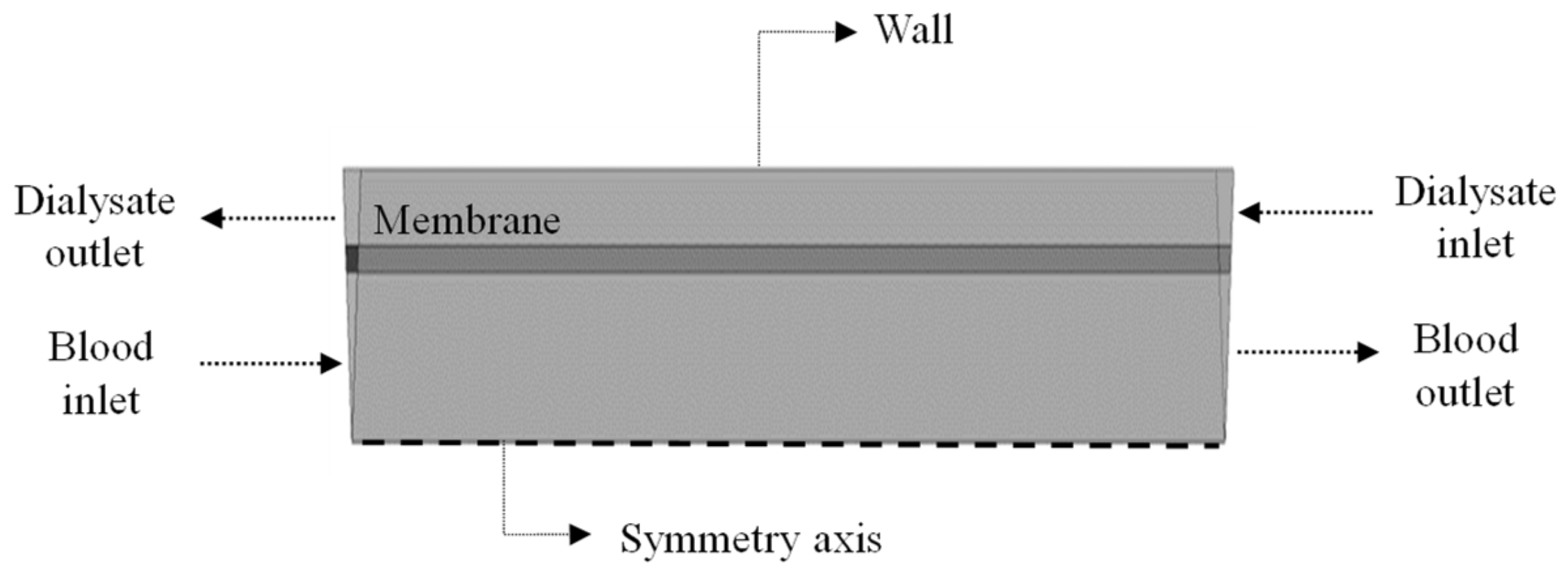
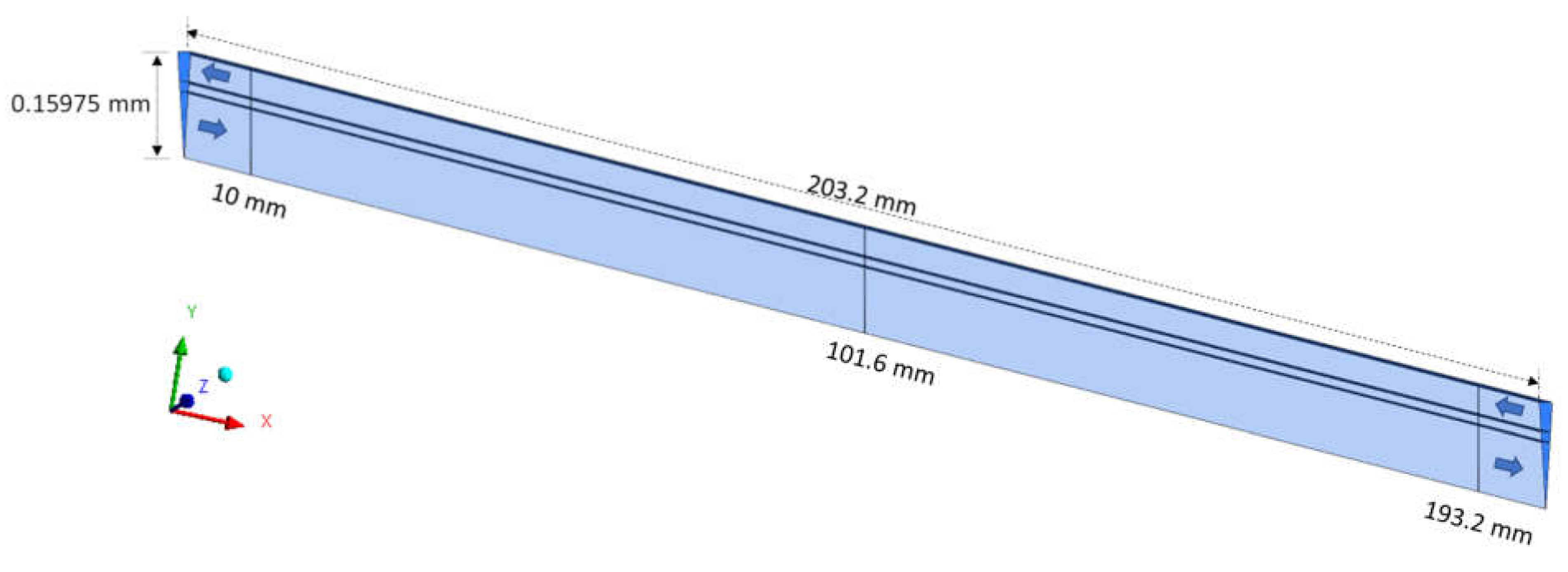
2.2. Computational Domain
2.3. Mathematical Modeling
- Newtonian fluids;
- Flow in a laminar, incompressible, isothermal, and transient regime;
- Constant thermophysical and chemical properties;
- Anisotropic porous medium;
- Negligible gravitational effect;
- The proteins present in the blood were disregarded;
- Adsorption of urea on the membrane contact surface, blockage of membrane pores, formation of concentration polarization layer, and chemical reactions are disregarded;
- Only one section of the hollow fiber membrane is considered, due to the angular symmetry presented by the geometry;
- The Eulerian–Eulerian approach was adopted for multiphase flow.
- Mass conservation equation for the non-porous media
- Linear momentum equation
- Linear momentum equation for the porous medium
Conditions Used in Simulations
- (a)
- Initial and boundary conditions
- Initial conditions
- Boundary conditions
- (b)
- Thermophysical parameters of membrane and fluids
2.4. Studied Cases
2.5. Procedures Used
- (a)
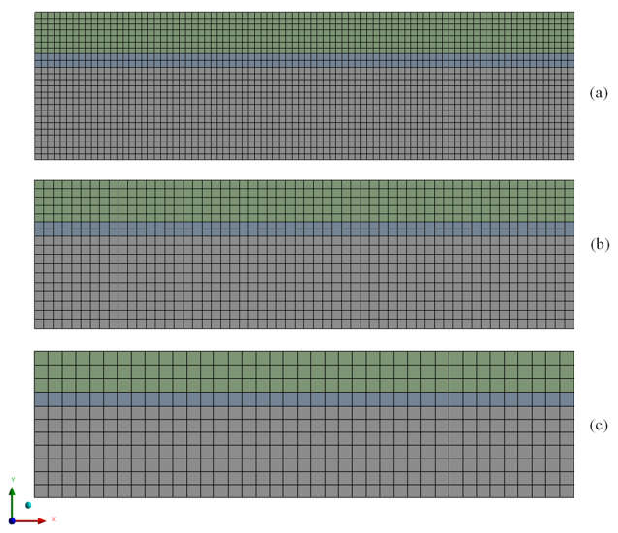
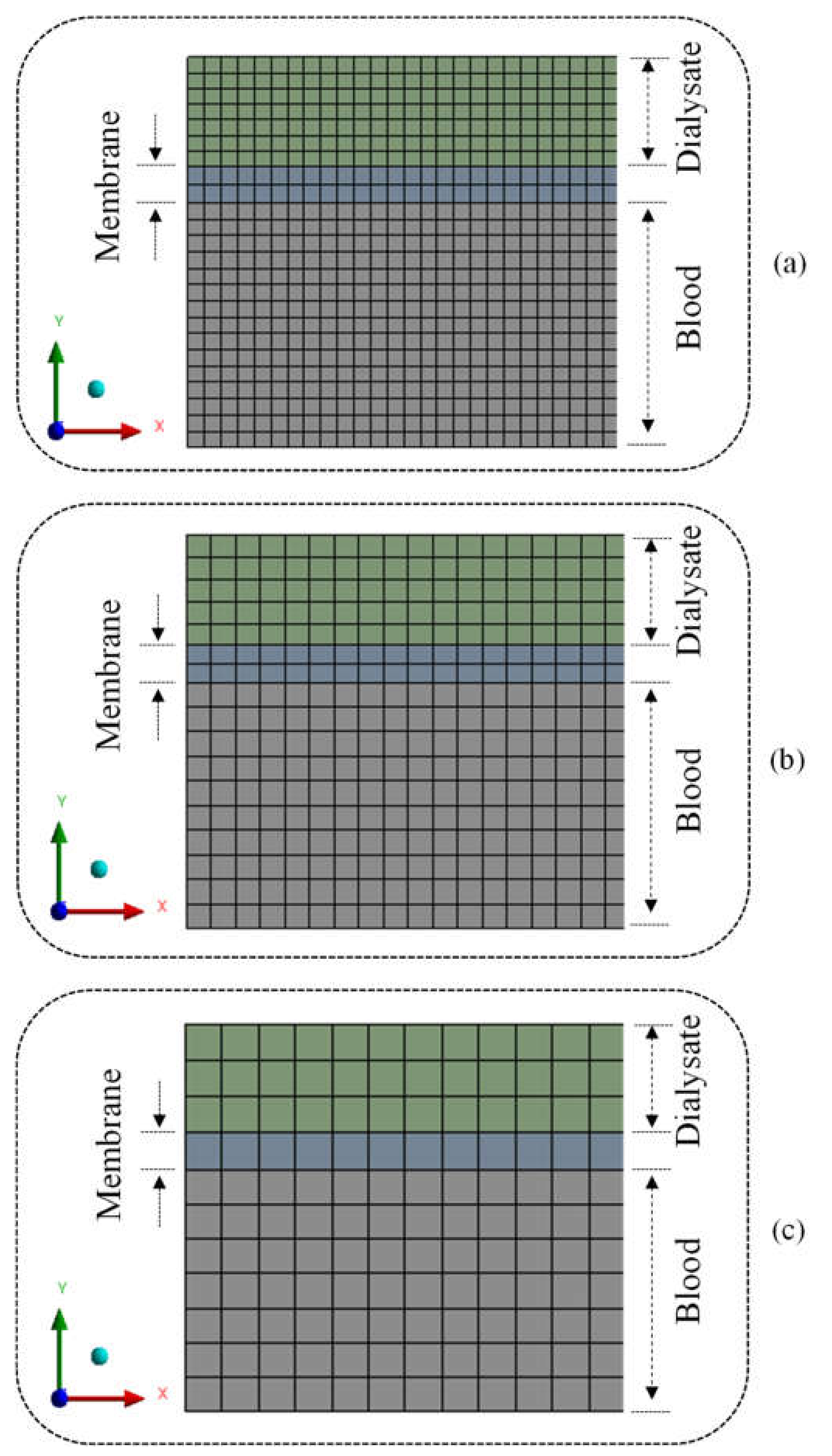
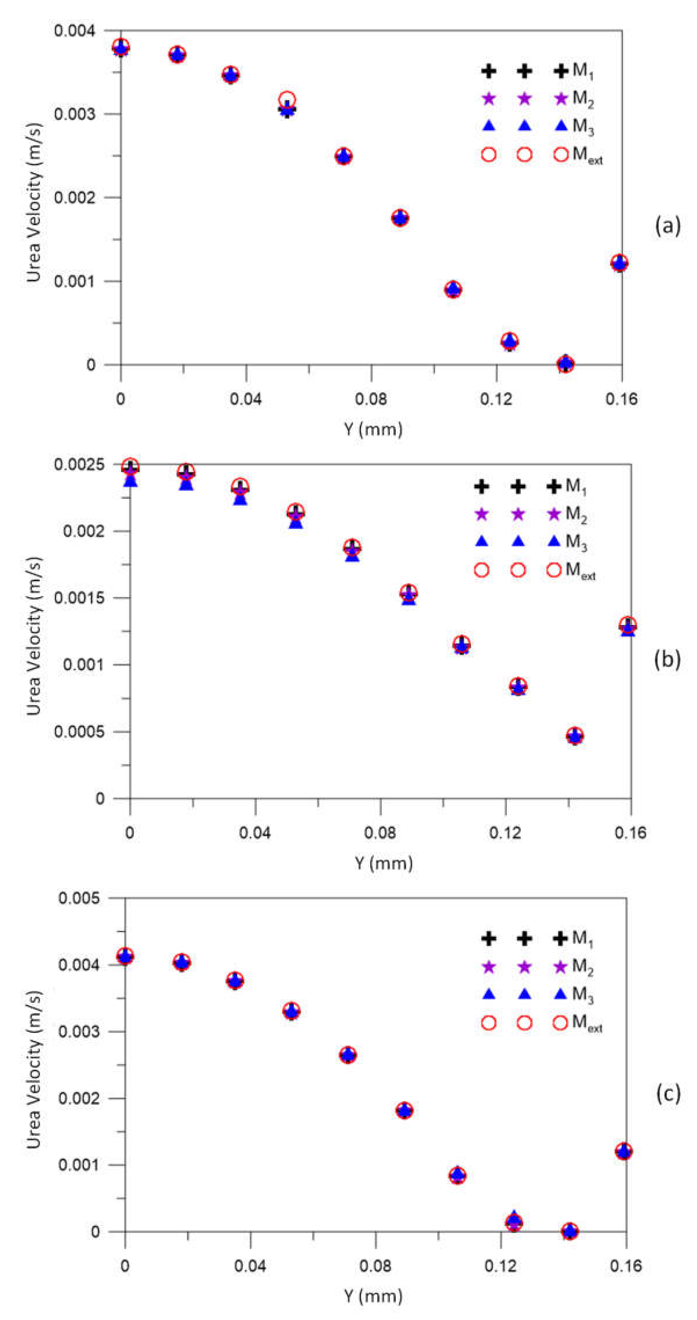
- Mesh evaluation
- (b)
- Validation of the mathematical model
3. Results and Discussion
3.1. Mesh Quality Assessment
3.2. Hollow Fiber Membrane Analysis
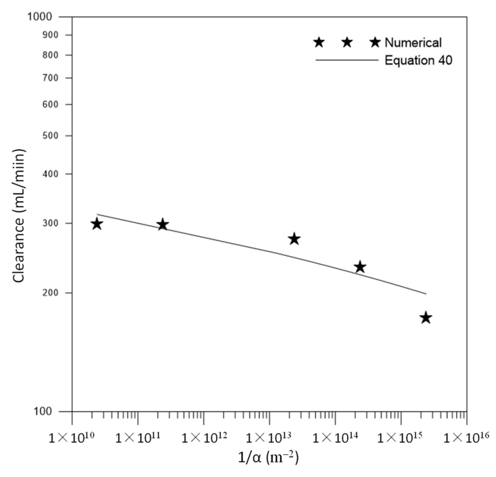
3.2.1. Clearance
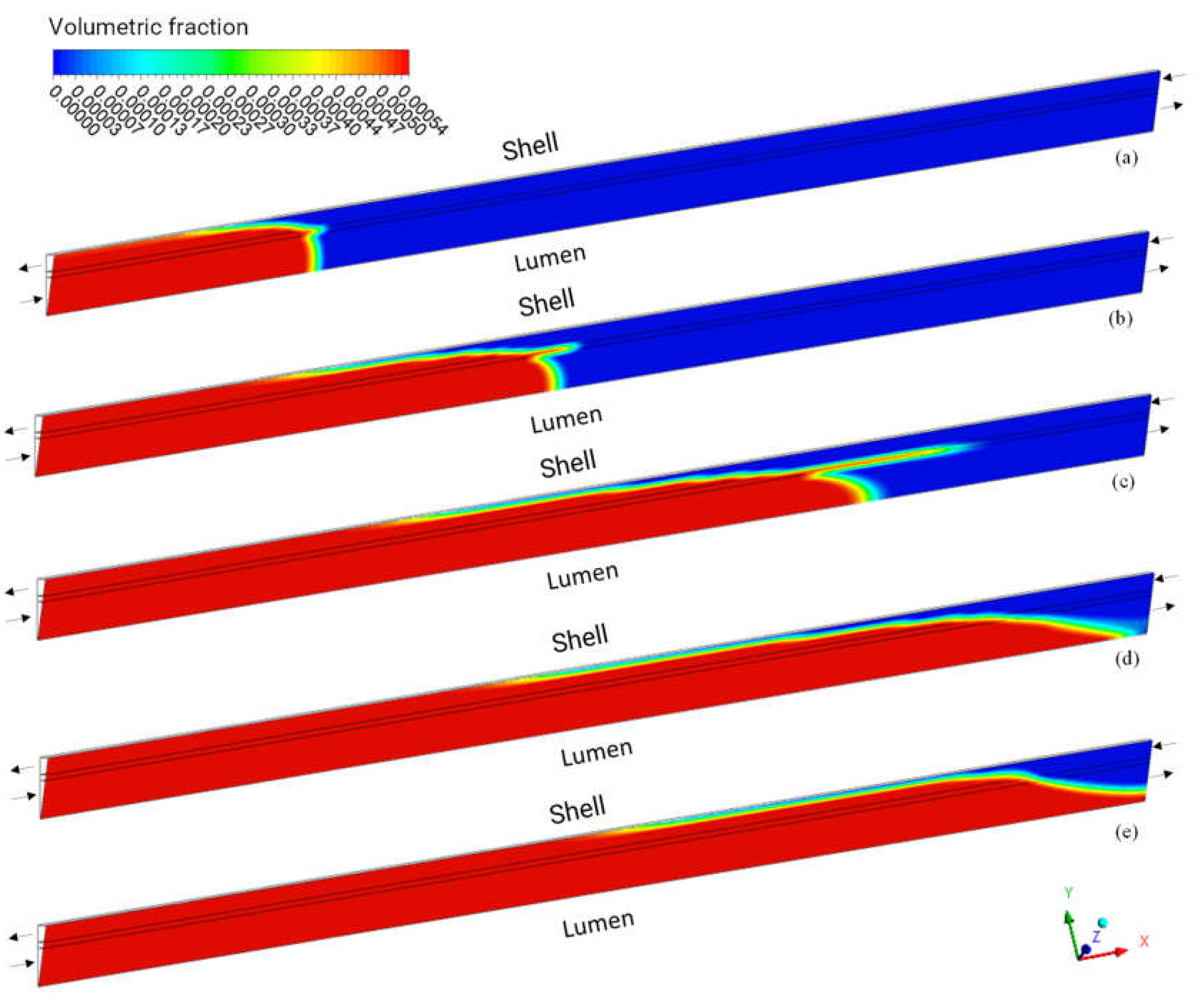
3.2.2. Volume Fraction
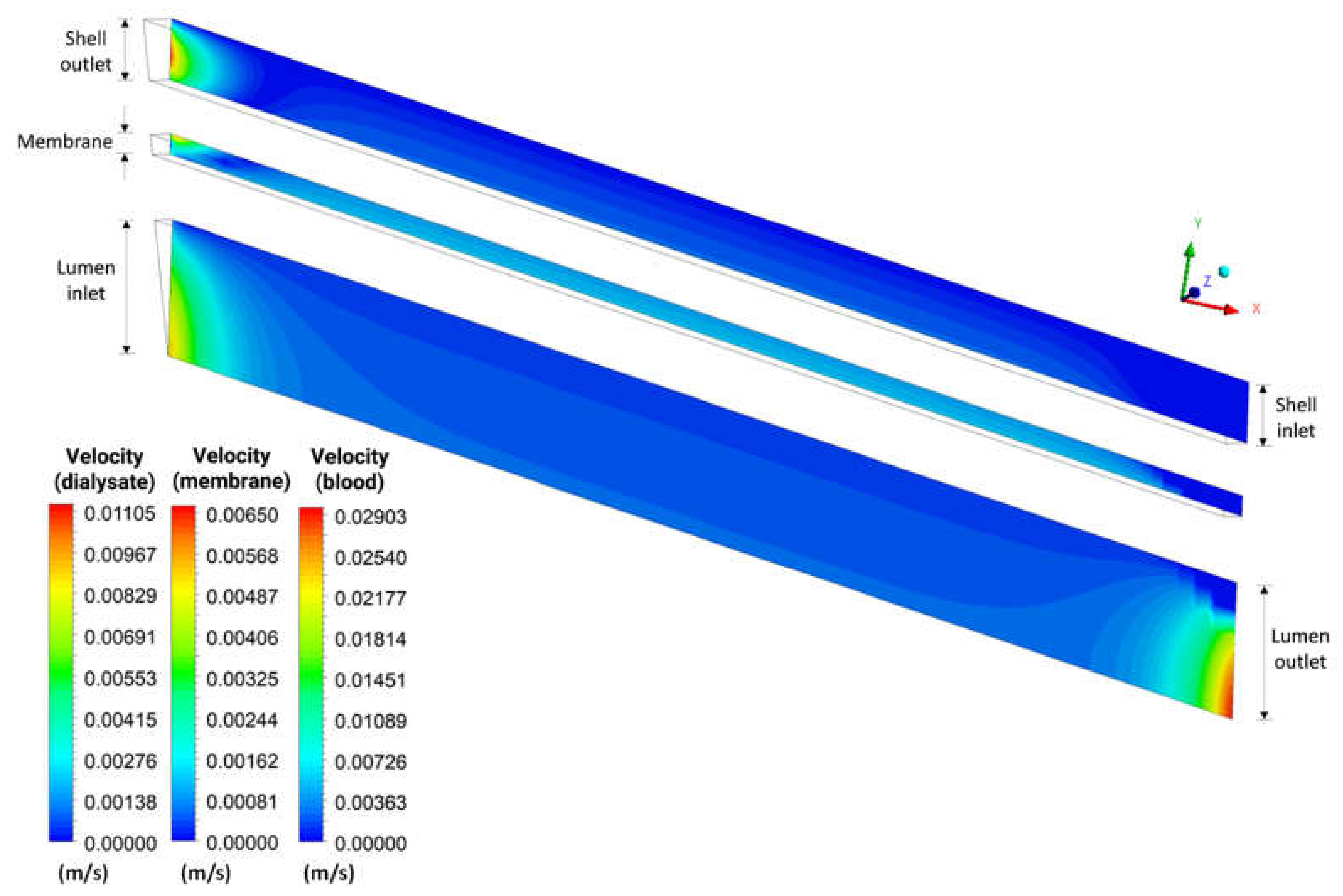
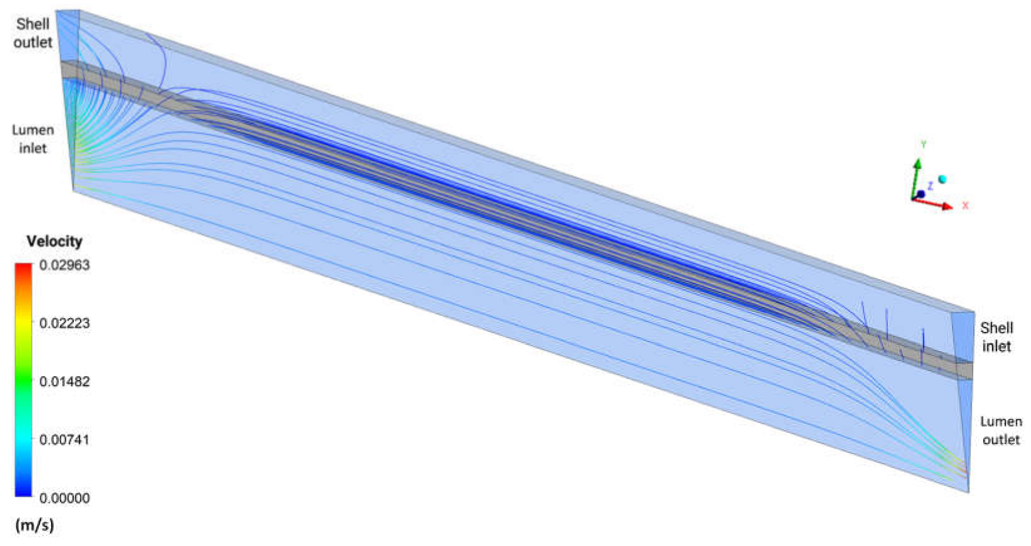
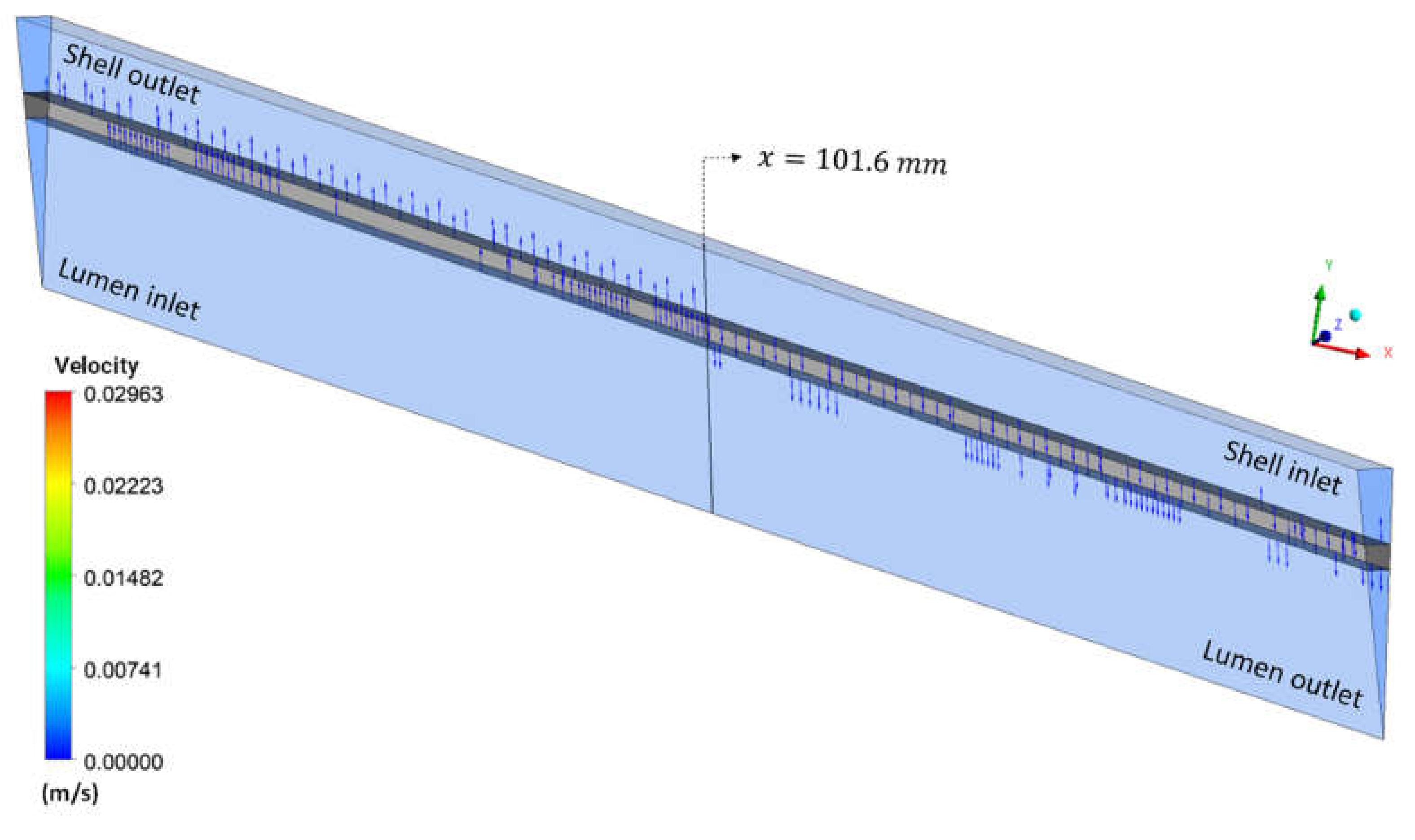
3.2.3. Flow Lines and Velocity Vectors
4. Conclusions
Author Contributions
Funding
Institutional Review Board Statement
Informed Consent Statement
Data Availability Statement
Acknowledgments
Conflicts of Interest
References
- Sesso, R.C.; Lopes, A.A.; Thomé, F.S.; Lugon, J.R.; Martins, C.T. Brazilian Chronic Dialysis Survey 2016. Braz. J. Nephrol. 2017, 39, 261–266. (In Portuguese) [Google Scholar] [CrossRef] [PubMed]
- Ribeiro, R.D.C.H.M.; Oliveira, G.A.S.A.; Ribeiro, D.F.; Bertolin, D.C.; Cesarino, C.B.; Lima, L.C.E.Q.; Oliveira, S.M. Characterization and etiology of chronic renal failure in a nephrology unit in the interior of the State of São Paulo. ACTA Paul. Enferm. 2008, 21, 207–211. (In Portuguese) [Google Scholar] [CrossRef]
- Kalra, S.; McBryde, C.W.; Lawrence, T. Intracapsular hip fractures in end-stage renal failure. Injury 2006, 37, 175–184. [Google Scholar] [CrossRef]
- Vanholder, R.; Smet, R.; Glorieux, G.; Argilés, A.; Baurmeister, U.; Brunet, P.; Clark, W.; Cohen, G.; Deyn, P.P.; Deppisch, R.; et al. Review on uremic toxins: Classification, concentration, and interindividual variability. Kidney Int. 2003, 63, 1934–1943. [Google Scholar] [CrossRef] [PubMed] [Green Version]
- De Rosa, S.; Prowle, J.R.; Samoni, S.; Villa, G.; Ronco, C. Acute kidney injury in patients with chronic kidney disease. In Critical Care Nephrology, 3rd ed.; Elsevier: Amsterdam, The Netherlands, 2019; pp. 85–89. [Google Scholar]
- Lu, J.; Lu, W.Q. A numerical simulation for mass transfer through the porous membrane of parallel straight channels. Int. J. Heat Mass Transf. 2010, 53, 2404–2413. [Google Scholar] [CrossRef]
- Lu, J.; Lu, W.-Q. Blood flow velocity and ultra-filtration velocity measured by CT imaging system inside a densely bundled hollow fiber dialyzer. Int. J. Heat Mass Transf. 2010, 53, 1844–1850. [Google Scholar] [CrossRef]
- Clark, W.R.; Gao, D.; Neri, M.; Ronco, C. Solute transport in hemodialysis: Advances and limitations of current membrane technology. In Expanded Hemodialysis; Karger Publishers: Basel, Switzerland, 2017; Volume 191, pp. 84–99. [Google Scholar]
- Ding, W.; Li, W.; Sun, S.; Zhou, X.; Hardy, P.A.; Ahmad, S.; Gao, D. Three-Dimensional Simulation of Mass Transfer in Artificial Kidneys. Artif. Organs 2015, 39, E79–E89. [Google Scholar] [CrossRef]
- Klein, E.; Holland, F.; Lebeouf, A.; Donnaud, A.; Smith, J.K. Transport and mechanical properties of hemodialysis hollow fibers. J. Membr. Sci. 1976, 1, 371–396. [Google Scholar] [CrossRef]
- Liao, Z.; Klein, E.; Poh, C.K.; Huang, Z.; Lu, J.; Hardy, P.A.; Gao, D. Measurement of hollow fiber membrane transport properties in hemodialyzers. J. Membr. Sci. 2005, 256, 176–183. [Google Scholar] [CrossRef]
- Lu, J.; Lu, W. An approximate analytical solution to the ultra-filtration profile in a hemodialysis process between parallel porous plates. Chin. Sci. Bull. 2008, 53, 3402–3408. [Google Scholar] [CrossRef] [Green Version]
- Pstras, L.; Stachowska-Pietka, J.; Debowska, M.; Pietribiasi, M.; Poleszczuk, J.; Waniewski, J. Dialysis therapies: Investigation of transport and regulatory processes using mathematical modelling. Biocybern. Biomed. Eng. 2022, 42, 60–78. [Google Scholar] [CrossRef]
- Cancilla, N.; Gurreri, L.; Marotta, G.; Ciofalo, M.; Cipollina, A.; Tamburini, A.; Micale, G. A porous media CFD model for the simulation of hemodialysis in hollow fiber membrane modules. J. Membr. Sci. 2022, 646, 120219. [Google Scholar] [CrossRef]
- Gostoli, C.; Gatta, A. Mass transfer in a hollow fiber dialyzer. J. Membr. Sci. 1980, 6, 133–148. [Google Scholar] [CrossRef]
- Ding, W.; He, L.; Zhao, G.; Shu, Z.; Cheng, S.; Gao, D. A novel theoretical model for mass transfer of hollow fiber hemodialyzers. Chin. Sci. Bull. 2003, 48, 2386–2390. [Google Scholar] [CrossRef]
- Kanchan, M.; Maniyeri, R. Computational Study of Fluid Flow in Wavy Channels Using Immersed Boundary Method. In Soft Computing for Problem Solving; Springer: Singapore, 2019; pp. 283–293. [Google Scholar]
- Liao, Z.; Poh, C.K.; Huang, Z.; Hardy, P.A.; Clark, W.R.; Gao, D. A numerical and experimental study of mass transfer in the artificial kidney. J. Biomech. Eng. 2003, 125, 472–480. [Google Scholar] [CrossRef] [PubMed]
- Donato, D.; Boschetti-de-Fierro, A.; Zweigart, C.; Kolb, M.; Eloot, S.; Storr, M.; Krause, B.; Leypoldt, K.; Segers, P. Optimization of dialyzer design to maximize solute removal with a two-dimensional transport model. J. Membr. Sci. 2017, 541, 519–528. [Google Scholar] [CrossRef]
- Choi, Y.K.; Kim, J.T.; Ryou, H.S. Investigation on the effect of hematocrit on unsteady hemodynamic characteristics in arteriovenous graft using the multiphase blood model. J. Mech. Sci. Technol. 2015, 29, 2565–2571. [Google Scholar] [CrossRef]
- Kim, J.C.; Cruz, D.; Garzotto, F.; Kaushik, M.; Teixeria, C.; Baldwin, M.; Baldwin, I.; Nalesso, F.; Kim, J.H.; Kang, E. Effects of dialysate flow configurations in continuous renal replacement therapy on solute removal: Computational modeling. Blood Purif. 2013, 35, 106–111. [Google Scholar] [CrossRef]
- ANSYS INC. ANSYS FLUENT Theory Guide; Release 15.0; Ansys Inc.: Canonsburg, PA, USA, 2013; Volume 15317. [Google Scholar]
- Celik, I.B.; Ghia, U.; Roache, P.J.; Freitas, C.J. Procedure for estimation and reporting of uncertainty due to discretization in CFD applications. J. Fluids Eng. -Trans. ASME 2008, 130, 1–4. [Google Scholar]
- Lira, D.S. Textile Industry Effluent Microfiltration Process Using Hollow Fiber Membrane-Modeling and Simulation. Master’s Thesis, Federal University of Campina Grande, Campina Grande, PB, Brazil, 2018. (In Portuguese). [Google Scholar]
- Paudel, S.; Saenger, N. Grid refinement study for three dimensional CFD model involving incompressible free surface flow and rotating object. Comput. Fluids 2017, 143, 134–140. [Google Scholar] [CrossRef]
- Roache, P.J. Perspective: A Method for Uniform Reporting of Grid Refinement Studies. J. Fluids Eng. 1994, 116, 405–413. [Google Scholar] [CrossRef]
- Celik, I.B.; Karatekin, O. Numerical experiments on application of Richardson extrapolation with nonuniform grids. ASME J. Fluids Eng. 1997, 119, 584–590. [Google Scholar] [CrossRef]
- Eloot, S. Experimental and Numerical Modeling of Dialysis. Ph.D. Thesis, Ghent University, Gent, Belgium, 2004. [Google Scholar]


| Equipment Dimensions (mm) | |
|---|---|
| Length | 203.2 |
| Section thickness | 0.0208962 |
| The thickness of the dialysate flow region | 0.04475 |
| Membrane thickness | 0.015 |
| Blood flow thickness | 0.1 |
| Fluids | Density (kg/m3) | Viscosity (kg/m·s) | Viscous Resistance Axial (m −2) | Porosity | |
|---|---|---|---|---|---|
| Dialysate | 998.2 | 0.001003 | - | - | |
| Blood | Water | 998.2 | 0.001003 | - | - |
| Urea | 1280.0 | 0.002300 | - | - | |
| Membrane | - | - | 0.2 | ||
| Case | Number of Mesh Elements |
|---|---|
| 01 | 718.920 |
| 02 | 344.267 |
| 03 | 147.785 |
| Parameter | Symbol | Value |
|---|---|---|
| Lumen feed flux (mL/min) | 300 | |
| Shell feed flux (mL/min) | 300 | |
| Axial viscous resistance (m−2) | ||
| Radial viscous resistance (m−2) | ||
| Urea concentration in the lumen feed (kg/m3) | 0.7 |
| Case | |
|---|---|
| 04 | |
| 05 | |
| 06 | |
| 07 | |
| 08 | |
| 09 |
| Parameter | Axial Position | |||
|---|---|---|---|---|
| = 20 mm | = 101.6 mm | = 183.2 mm | ||
| Urea velocity (m/s) | Mesh M1 | |||
| Mesh M2 | ||||
| Mesh M3 | ||||
| (m/s) | ||||
| Mesh | Mean Relative Error (%) | ||
|---|---|---|---|
| (20 mm) | (101.6 mm) | (183.2 mm) | |
| 1.44 | 0.82 | 0.2 | |
| 2.04 | 1.66 | 0.36 | |
| 1.50 | 3.86 | 0.59 | |
| Parameter | Axial Position | |||
|---|---|---|---|---|
| = 10.0 mm | = 101.6 mm | = 193.2 mm | ||
| Pressure (Pa) | Mesh M1 | 188.42 | 135.71 | 80.58 |
| Mesh M2 | 185.58 | 134.78 | 81.96 | |
| Mesh M3 | 177.54 | 132.85 | 87.39 | |
| 1.598 | 1.030 | 2.205 | ||
| (Pa) | 190.81 | 137.14 | 79.88 | |
| 0.350 | 0.483 | 0.252 | ||
| Mesh | Mean Relative Error (%) | ||
|---|---|---|---|
(10.0 mm) | (101.6 mm) | (193.2 mm) | |
| M1 | 1.46 | 1.04 | 1.17 |
| M2 | 2.30 | 1.72 | 1.56 |
| M3 | 4.00 | 3.13 | 1.90 |
Publisher’s Note: MDPI stays neutral with regard to jurisdictional claims in published maps and institutional affiliations. |
© 2022 by the authors. Licensee MDPI, Basel, Switzerland. This article is an open access article distributed under the terms and conditions of the Creative Commons Attribution (CC BY) license (https://creativecommons.org/licenses/by/4.0/).
Share and Cite
Magalhães, H.L.F.; Gomez, R.S.; Leite, B.E.; Nascimento, J.B.S.; Brito, M.K.T.; Araújo, M.V.; Cavalcante, D.C.M.; Lima, E.S.; Lima, A.G.B.; Farias Neto, S.R. Investigating the Dialysis Treatment Using Hollow Fiber Membrane: A New Approach by CFD. Membranes 2022, 12, 710. https://doi.org/10.3390/membranes12070710
Magalhães HLF, Gomez RS, Leite BE, Nascimento JBS, Brito MKT, Araújo MV, Cavalcante DCM, Lima ES, Lima AGB, Farias Neto SR. Investigating the Dialysis Treatment Using Hollow Fiber Membrane: A New Approach by CFD. Membranes. 2022; 12(7):710. https://doi.org/10.3390/membranes12070710
Chicago/Turabian StyleMagalhães, Hortência L. F., Ricardo S. Gomez, Boniek E. Leite, Jéssica B. S. Nascimento, Mirenia K. T. Brito, Morgana V. Araújo, Daniel C. M. Cavalcante, Elisiane S. Lima, Antonio G. B. Lima, and Severino R. Farias Neto. 2022. "Investigating the Dialysis Treatment Using Hollow Fiber Membrane: A New Approach by CFD" Membranes 12, no. 7: 710. https://doi.org/10.3390/membranes12070710