
Modeling the Conductivity and Diffusion Permeability of a Track-Etched Membrane Taking into Account a Loose Layer
 ,
,  ,
,
Abstract
:1. Introduction
2. Theoretical
2.1. Basic Microheterogeneous Model (MHM)
2.2. Problem Formulation
3. Experimental
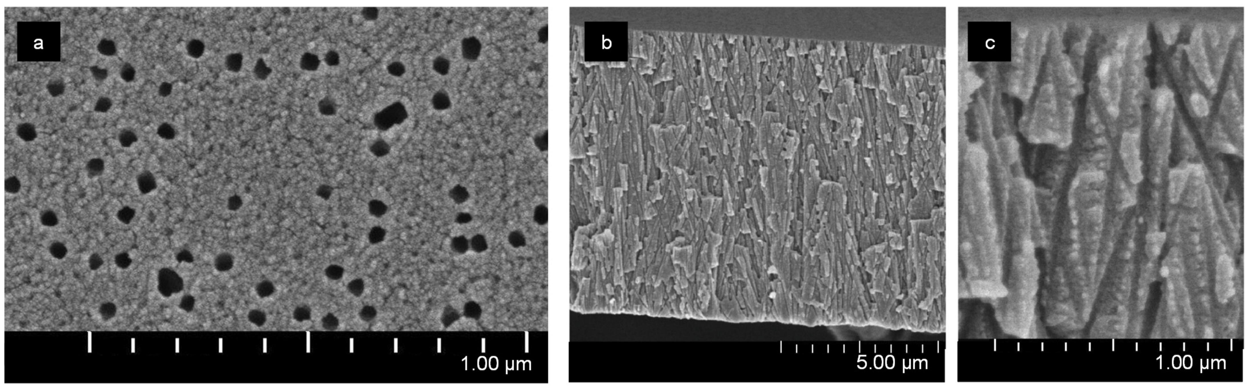
3.1. Membrane
3.2. Solution
3.3. Measurement of Transport Characteristics
3.4. Ion-Exchange Capacity
3.5. Zeta Potential
4. Results and Discussion
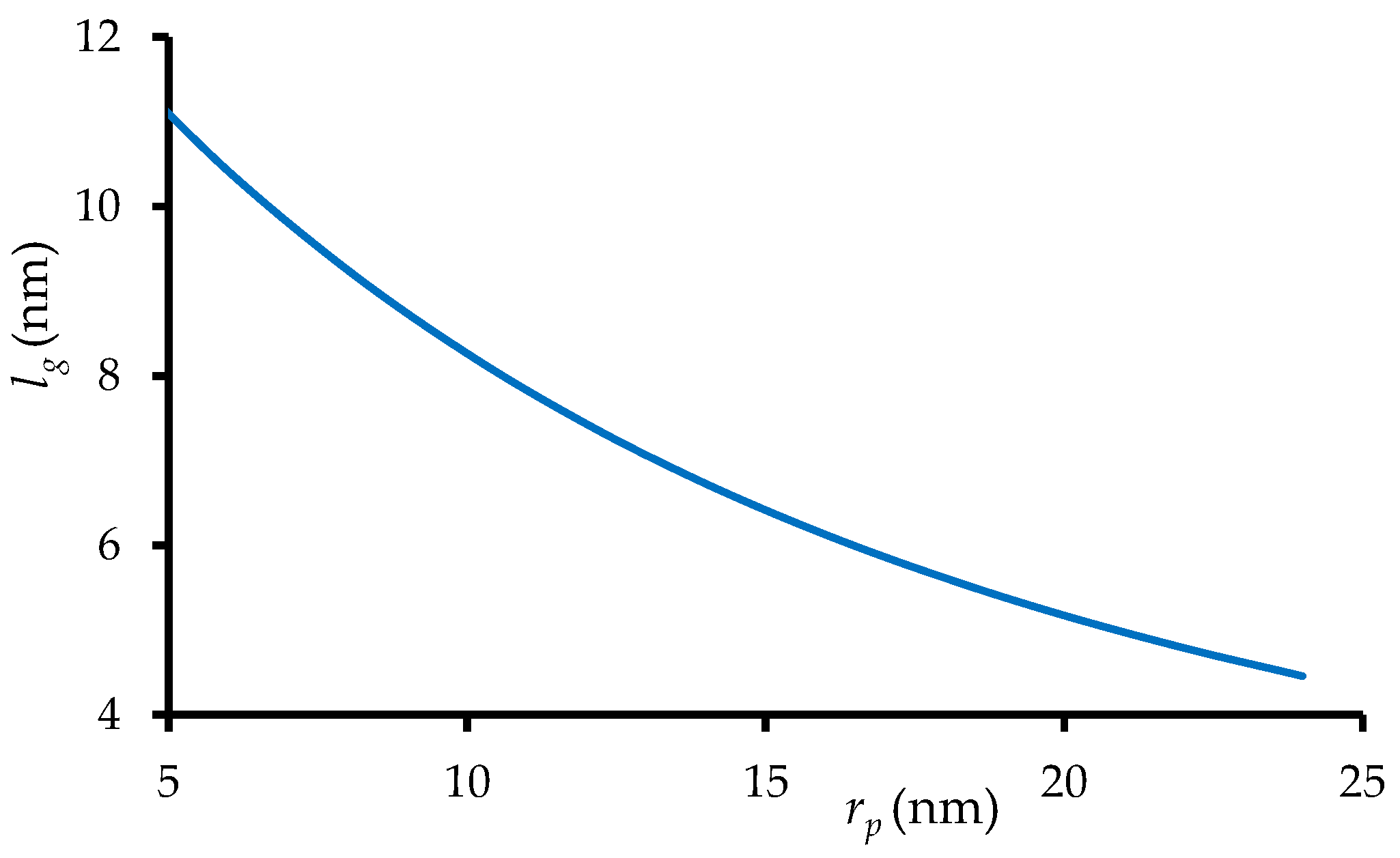
4.1. Model Input Parameters
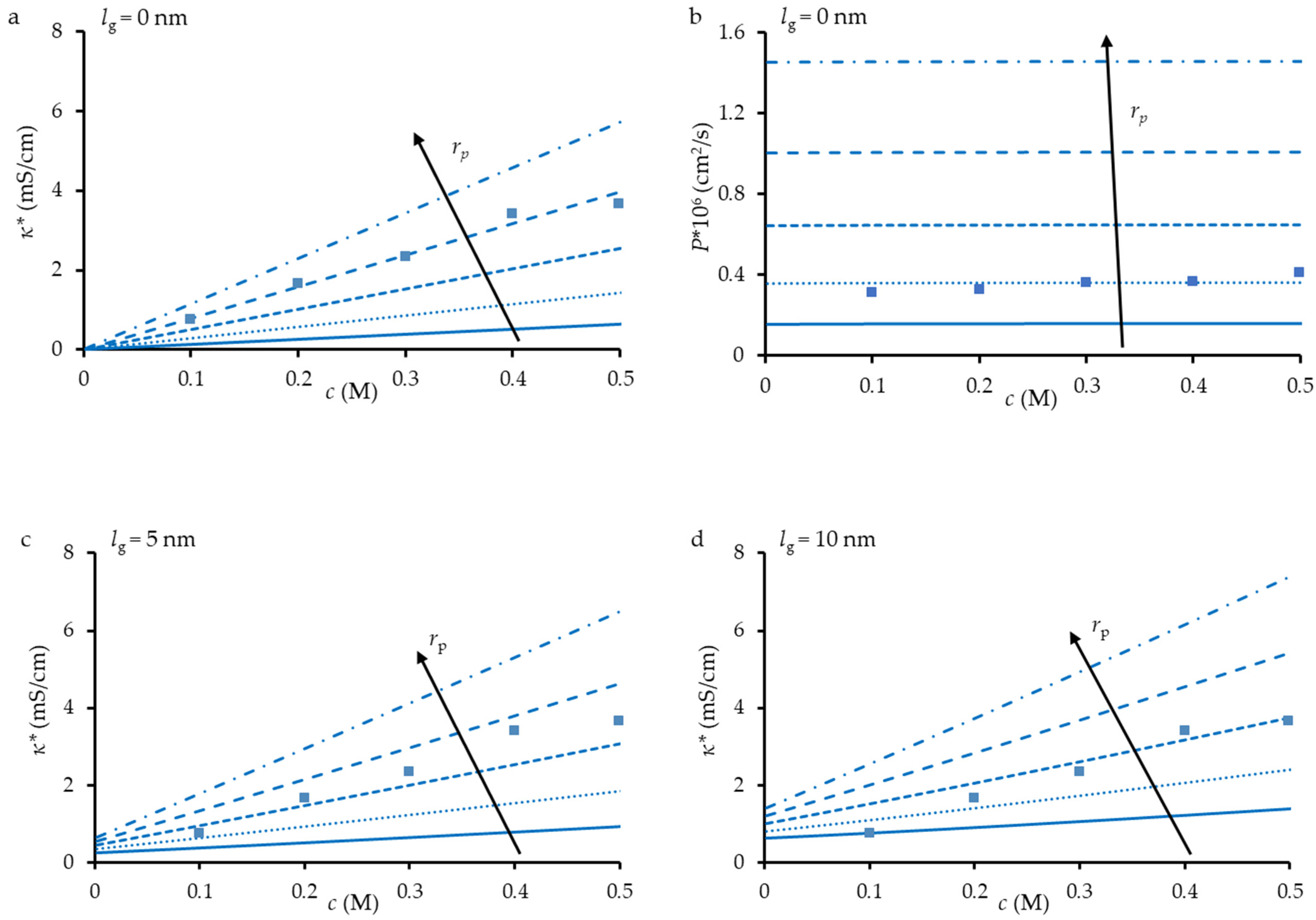
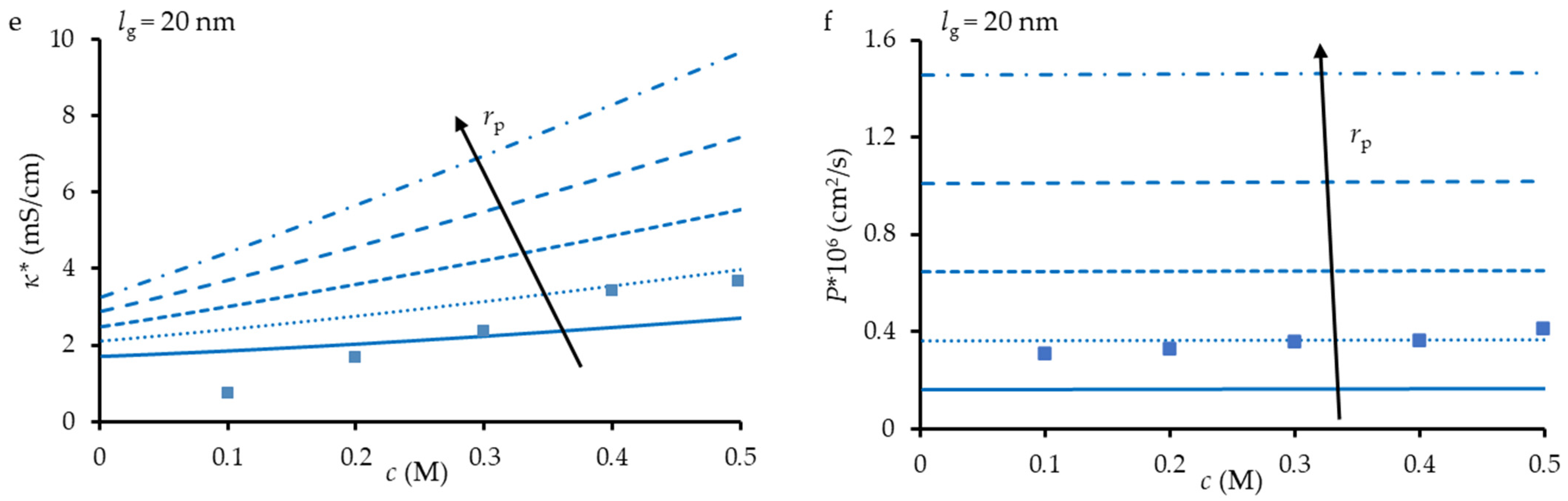
4.2. Modelling of Transport Characteristics for Cylindrical Pores Perpendicular to the Surface
4.3. Application of the MHM with α < 1
5. Conclusions
Author Contributions
Funding
Institutional Review Board Statement
Data Availability Statement
Acknowledgments
Conflicts of Interest
Appendix A
References
- Apel, P. Track etching technique in membrane technology. Radiat. Meas. 2001, 34, 559–566. [Google Scholar] [CrossRef]
- Karl, D.M. Plastics-Irradiated-Etched: The Nuclepore® Filter Turns 45 Years Old. Limnol. Oceanogr. Bull. 2007, 16, 49–54. [Google Scholar] [CrossRef]
- Apel, P.Y.; Bobreshova, O.V.; Volkov, A.V.; Volkov, V.V.; Nikonenko, V.V.; Stenina, I.A.; Filippov, A.N.; Yampolskii, Y.P.; Yaroslavtsev, A.B. Prospects of Membrane Science Development. Membr. Membr. Technol. 2019, 1, 45–63. [Google Scholar] [CrossRef] [Green Version]
- Dolfus, C.; Piton, N.; Toure, E.; Sabourin, J.C. Circulating tumor cell isolation: The assets of filtration methods with polycarbonate track-etched filters. Chin. J. Cancer Res. 2015, 27, 479–487. [Google Scholar] [CrossRef]
- Kaya, D.; Keçeci, K. Review—Track-Etched Nanoporous Polymer Membranes as Sensors: A Review. J. Electrochem. Soc. 2020, 167, 037543. [Google Scholar] [CrossRef]
- Novo, P.; Dell’Aica, M.; Jender, M.; Höving, S.; Zahedi, R.P.; Janasek, D. Integration of polycarbonate membranes in microfluidic free-flow electrophoresis. Analyst 2017, 142, 4228–4239. [Google Scholar] [CrossRef]
- Martínez-Pérez, P.; García-Rupérez, J. Commercial polycarbonate track-etched membranes as substrates for low-cost optical sensors. Beilstein J. Nanotechnol. 2019, 10, 677–683. [Google Scholar] [CrossRef] [Green Version]
- Martin, C.R. Nanomaterials: A Membrane-Based Synthetic Approach. Science 1994, 266, 1961–1966. [Google Scholar] [CrossRef]
- Dutt, S.; Apel, P.; Lizunov, N.; Notthoff, C.; Wen, Q.; Trautmann, C.; Mota-Santiago, P.; Kirby, N.; Kluth, P. Shape of nanopores in track-etched polycarbonate membranes. J. Memb. Sci. 2021, 638, 119681. [Google Scholar] [CrossRef]
- Apel, P.Y.; Blonskaya, I.V.; Ivanov, O.M.; Kristavchuk, O.V.; Nechaev, A.N.; Olejniczak, K.; Orelovich, O.L.; Polezhaeva, O.A.; Dmitriev, S.N. Do the soft-etched and UV-track membranes actually have uniform cylindrical subnanometer channels? Radiat. Phys. Chem. 2022, 198, 110266. [Google Scholar] [CrossRef]
- Hernandez, A.; Martinez-villa, F.; Ibañez, J.A.; Arribas, J.I.; Tejerina, A.F. An Experimentally Fitted and Simple Model for the Pores in Nuclepore Membranes. Sep. Sci. Technol. 1986, 21, 665–677. [Google Scholar] [CrossRef]
- Schönenberger, C.; van der Zande, B.M.I.; Fokkink, L.G.J.; Henny, M.; Schmid, C.; Krüger, M.; Bachtold, A.; Huber, R.; Birk, H.; Staufer, U. Template Synthesis of Nanowires in Porous Polycarbonate Membranes: Electrochemistry and Morphology. J. Phys. Chem. B 1997, 101, 5497–5505. [Google Scholar] [CrossRef]
- Duchet, J.; Legras, R.; Demoustier-Champagne, S. Chemical synthesis of polypyrrole: Structure–properties relationship. Synth. Met. 1998, 98, 113–122. [Google Scholar] [CrossRef]
- Ferain, E.; Legras, R. Characterisation of nanoporous particle track etched membrane. Nucl. Instrum. Methods Phys. Res. Sect. B Beam Interact. Mater. At. 1997, 131, 97–102. [Google Scholar] [CrossRef]
- Déjardin, P.; Vasina, E.N.; Berezkin, V.V.; Sobolev, V.D.; Volkov, V.I. Streaming Potential in Cylindrical Pores of Poly(ethylene terephthalate) Track-Etched Membranes: Variation of Apparent ζ Potential with Pore Radius. Langmuir 2005, 21, 4680–4685. [Google Scholar] [CrossRef]
- Apel, P.Y.; Blonskaya, I.V.; Dmitriev, S.N.; Orelovich, O.L.; Sartowska, B.A. Ion track symmetric and asymmetric nanopores in polyethylene terephthalate foils for versatile applications. Nucl. Instrum. Methods Phys. Res. Sect. B Beam Interact. Mater. At. 2015, 365, 409–413. [Google Scholar] [CrossRef]
- Apel, P.Y. Track-Etching. In Encyclopedia of Membrane Science and Technology; Hoek, E.M.V., Tarabara, V.V., Eds.; John Wiley & Sons, Inc.: Hoboken, NJ, USA, 2013; pp. 332–355. [Google Scholar]
- Fink, D.; Dwivedi, K.K.; Müller, M.; Ghosh, S.; Hnatowicz, V.; Vacik, J.; Červena, J. On the penetration of etchant into tracks in polycarbonate. Radiat. Meas. 2000, 32, 307–313. [Google Scholar] [CrossRef]
- Fink, D.; Petrov, A.; Müller, M.; Asmus, T.; Hnatowicz, V.; Vacik, J.; Cervena, J. Electrolyte penetration into high energy ion irradiated polymers. Surf. Coat. Technol. 2002, 158–159, 228–233. [Google Scholar] [CrossRef]
- Apel, P.; Koter, S.; Yaroshchuk, A. Time-resolved pressure-induced electric potential in nanoporous membranes: Measurement and mechanistic interpretation. J. Memb. Sci. 2022, 653, 120556. [Google Scholar] [CrossRef]
- Berezkin, V.V.; Volkov, V.I.; Kiseleva, O.A.; Mitrofanova, N.V.; Sobolev, V.D. Electrosurface properties of poly(ethylene terephtalate) track membranes. Adv. Colloid Interface Sci. 2003, 104, 325–331. [Google Scholar] [CrossRef]
- Apel, P.; Schulz, A.; Spohr, R.; Trautmann, C.; Vutsadakis, V. Track size and track structure in polymer irradiated by heavy ions. Nucl. Instrum. Methods Phys. Res. Sect. B Beam Interact. Mater. At. 1998, 146, 468–474. [Google Scholar] [CrossRef]
- Apel, P.Y.; Blonskaya, I.V.; Ivanov, O.M.; Kristavchuk, O.V.; Lizunov, N.E.; Nechaev, A.N.; Orelovich, O.L.; Polezhaeva, O.A.; Dmitriev, S.N. Creation of Ion-Selective Membranes from Polyethylene Terephthalate Films Irradiated with Heavy Ions: Critical Parameters of the Process. Membr. Membr. Technol. 2020, 2, 98–108. [Google Scholar] [CrossRef] [Green Version]
- Blonskaya, I.V.; Kristavchuk, O.V.; Nechaev, A.N.; Orelovich, O.L.; Polezhaeva, O.A.; Apel, P.Y. Observation of latent ion tracks in semicrystalline polymers by scanning electron microscopy. J. Appl. Polym. Sci. 2021, 138, 49869. [Google Scholar] [CrossRef]
- Sabbatovsky, K.G.; Vilensky, A.I.; Sobolev, V.D.; Mchedlishvili, B.V. Influence of thermal treatment on electrosurface and structural properties of poly(ethylene terephthalate) track membranes. Pet. Chem. 2012, 52, 480–486. [Google Scholar] [CrossRef]
- Okada, T.; Matsuura, T. A new transport model for pervaporation. J. Memb. Sci. 1991, 59, 133–149. [Google Scholar] [CrossRef]
- Sukitpaneenit, P.; Chung, T.S.; Jiang, L.Y. Modified pore-flow model for pervaporation mass transport in PVDF hollow fiber membranes for ethanol-water separation. J. Memb. Sci. 2010, 362, 393–406. [Google Scholar] [CrossRef]
- Wijmans, J.G.; Baker, R.W. The solution-diffusion model: A review. J. Memb. Sci. 1995, 107, 1–21. [Google Scholar] [CrossRef]
- Selvey, C.; Reiss, H. Ion transport in inhomogeneous ion exchange membranes. J. Memb. Sci. 1985, 23, 11–27. [Google Scholar] [CrossRef]
- Xu, T.W.; Li, Y.; Wu, L.; Yang, W.H. A simple evaluation of microstructure and transport parameters of ion-exchange membranes from conductivity measurements. Sep. Purif. Technol. 2008, 60, 73–80. [Google Scholar] [CrossRef]
- Zabolotsky, V.I.; Nikonenko, V.V. Effect of structural membrane inhomogeneity on transport properties. J. Memb. Sci. 1993, 79, 181–198. [Google Scholar] [CrossRef]
- Pismenskaya, N.D.; Nevakshenova, E.E.; Nikonenko, V.V. Using a Single Set of Structural and Kinetic Parameters of the Microheterogeneous Model to Describe the Sorption and Kinetic Properties of Ion-Exchange Membranes. Pet. Chem. 2018, 58, 465–473. [Google Scholar] [CrossRef]
- De Jaegher, B.; De Schepper, W.; Verliefde, A.; Nopens, I. A model-based analysis of electrodialysis fouling during pulsed electric field operation. J. Memb. Sci. 2022, 642, 119975. [Google Scholar] [CrossRef]
- Sarapulova, V.V.; Pasechnaya, E.L.; Titorova, V.D.; Pismenskaya, N.D.; Apel, P.Y.; Nikonenko, V.V. Electrochemical Properties of Ultrafiltration and Nanofiltration Membranes in Solutions of Sodium and Calcium Chloride. Membr. Membr. Technol. 2020, 2, 332–350. [Google Scholar] [CrossRef]
- Khoiruddin, K.; Ariono, D.; Subagjo, S.; Wenten, I.G. The effect of heterogeneity in ion-exchange membrane structure on Donnan Exclusion. J. Phys. Conf. Ser. 2018, 1090, 012045. [Google Scholar] [CrossRef]
- Salmeron-Sanchez, I.; Asenjo-Pascual, J.; Avilés-Moreno, J.R.; Ocón, P. Microstructural description of ion exchange membranes: The effect of PPy-based modification. J. Memb. Sci. 2022, 659, 120771. [Google Scholar] [CrossRef]
- Kozmai, A.; Pismenskaya, N.; Nikonenko, V. Mathematical Description of the Increase in Selectivity of an Anion-Exchange Membrane Due to Its Modification with a Perfluorosulfonated Ionomer. Int. J. Mol. Sci. 2022, 23, 2238. [Google Scholar] [CrossRef]
- Loza, S.; Loza, N.; Kutenko, N.; Smyshlyaev, N. Profiled Ion-Exchange Membranes for Reverse and Conventional Electrodialysis. Membranes 2022, 12, 985. [Google Scholar] [CrossRef]
- Khoiruddin, K.; Ariono, D.; Subagjo, S.; Wenten, I.G. Structure and transport properties of polyvinyl chloride-based heterogeneous cation-exchange membrane modified by additive blending and sulfonation. J. Electroanal. Chem. 2020, 873, 114304. [Google Scholar] [CrossRef]
- Choy, T.C. Effective Medium Theory; Oxford University Press: Oxford, UK, 2015; Volume 165, ISBN 9780198705093. [Google Scholar]
- Nikonenko, V.; Nebavsky, A.; Mareev, S.; Kovalenko, A.; Urtenov, M.; Pourcelly, G. Modelling of ion transport in electromembrane systems: Impacts of membrane bulk and surface heterogeneity. Appl. Sci. 2018, 9, 25. [Google Scholar] [CrossRef] [Green Version]
- Zabolotskii, V.V.; Nikonenko, V.V. Ion Transport in Membranes (in Russian); Nauka: Moscow, Russia, 1996; ISBN 5-02-001677-2. [Google Scholar]
- Auclair, B.; Nikonenko, V.; Larchet, C.; Métayer, M.; Dammak, L. Correlation between transport parameters of ion-exchange membranes. J. Memb. Sci. 2001, 195, 89–102. [Google Scholar] [CrossRef]
- Butylskii, D.Y.; Pismenskaya, N.D.; Apel, P.Y.; Sabbatovskiy, K.G.; Nikonenko, V. V Highly selective separation of singly charged cations by countercurrent electromigration with a track-etched membrane. J. Memb. Sci. 2021, 635, 119449. [Google Scholar] [CrossRef]
- Kravets, L.I.; Dmitriev, S.N.; Apel, P.Y. The properties and porous structure of polypropylene track membranes. Radiat. Meas. 1995, 25, 729–732. [Google Scholar] [CrossRef]
- Berezina, N.P.; Kononenko, N.A.; Dyomina, O.A.; Gnusin, N.P. Characterization of ion-exchange membrane materials: Properties vs structure. Adv. Colloid Interface Sci. 2008, 139, 3–28. [Google Scholar] [CrossRef] [PubMed]
- Lteif, R.; Dammak, L.; Larchet, C.; Auclair, B. Conductivité électrique membranaire: Étude de l’effet de la concentration, de la nature de l’electrolyte et de la structure membranaire. Eur. Polym. J. 1999, 35, 1187–1195. [Google Scholar] [CrossRef]
- Karpenko, L.V.; Demina, O.A.; Dvorkina, G.A.; Parshikov, S.B.; Larchet, C.; Auclair, B.; Berezina, N.P. Comparative study of methods used for the determination of electroconductivity of ion-exchange membranes. Russ. J. Electrochem. 2001, 37, 287–293. [Google Scholar] [CrossRef]
- Helfferich, F.G. Ion Exchange; Dover Publications: Mineola, NY, USA, 1995; ISBN 0486687848. [Google Scholar]
- Butt, H.; Graf, K.; Kappl, M. Physics and Chemistry of Interfaces; Wiley: Weinheim, Germany, 2003; ISBN 9783527404131. [Google Scholar]
- Roques, H. Fondements Théoriques du Traitement Chimique des Eaux; Lavoisier: Paris, France, 1990; Volume 1, ISBN 2852066149. [Google Scholar]
- Lide, D.R.; Baysinger, G.; Berger, L.I.; Kehiaian, H.V.; Roth, D.L.; Zwillinger, D.; Goldberg, R.N.; Haynes, W.M. CRC Handbook of Chemistry and Physics, 89th Edition (Internet Version 2009); Lide, D.R., Ed.; CRC Press/Taylor and Francis: Boca Raton, FL, USA, 2009; Volume 268. [Google Scholar]
- Sanborn, C.D.; Chacko, J.V.; Digman, M.; Ardo, S. Interfacial and Nanoconfinement Effects Decrease the Excited-State Acidity of Polymer-Bound Photoacids. Chem 2019, 5, 1648–1670. [Google Scholar] [CrossRef]
- Chen, W.; McCarthy, T.J. Chemical Surface Modification of Poly(ethylene terephthalate). Macromolecules 1998, 31, 3648–3655. [Google Scholar] [CrossRef]
- Titorova, V.D.; Moroz, I.A.; Mareev, S.A.; Pismenskaya, N.D.; Sabbatovskii, K.G.; Wang, Y.; Xu, T.; Nikonenko, V.V. How bulk and surface properties of sulfonated cation-exchange membranes response to their exposure to electric current during electrodialysis of a Ca2+ containing solution. J. Memb. Sci. 2022, 644, 120149. [Google Scholar] [CrossRef]
- Sedkaoui, Y.; Szymczyk, A.; Lounici, H.; Arous, O. A new lateral method for characterizing the electrical conductivity of ion-exchange membranes. J. Memb. Sci. 2016, 507, 34–42. [Google Scholar] [CrossRef]
- Sarapulova, V.V.; Titorova, V.D.; Nikonenko, V.V.; Pismenskaya, N.D. Transport Characteristics of Homogeneous and Heterogeneous Ion-Exchange Membranes in Sodium Chloride, Calcium Chloride, and Sodium Sulfate Solutions. Membr. Membr. Technol. 2019, 1, 168–182. [Google Scholar] [CrossRef]
- Güler, E.; van Baak, W.; Saakes, M.; Nijmeijer, K. Monovalent-ion-selective membranes for reverse electrodialysis. J. Memb. Sci. 2014, 455, 254–270. [Google Scholar] [CrossRef]
- Kozmai, A.E.; Nikonenko, V.V.; Zyryanova, S.; Pismenskaya, N.D.; Dammak, L. A simple model for the response of an anion-exchange membrane to variation in concentration and pH of bathing solution. J. Memb. Sci. 2018, 567, 127–138. [Google Scholar] [CrossRef]
- Kislyi, A.G.; Butylskii, D.Y.; Mareev, S.A.; Nikonenko, V.V. Model of Competitive Ion Transfer in an Electro-Baromembrane System with Track-Etched Membrane. Membr. Membr. Technol. 2021, 3, 131–138. [Google Scholar] [CrossRef]
- Salmeron-Sanchez, I.; Asenjo-Pascual, J.; Avilés-Moreno, J.R.; Pérez-Flores, J.C.; Mauleón, P.; Ocón, P. Chemical physics insight of PPy-based modified ion exchange membranes: A fundamental approach. J. Memb. Sci. 2022, 643, 120020. [Google Scholar] [CrossRef]


| Thickness * | Pore Density *, np | Pore Radius, rp | Surface Porosity | Fixed Groups [17] | |||
| 10 μm | 5.0 × 10⁹ pores/cm2 | 20 nm * 14 nm ** 22 nm *** | 0.063 | hydroxyl and carboxyl groups | |||
| Water Uptake [34] | Hydraulic Permeability [44] | Density (Dry) [44] | Total Ion-Exchange Capacity, Qtotmb [34] | ||||
| 5% | 5.0 × 10⁻³ cm3/(cm2 min) | 1.30 ± 0.02 g cm−3 | 0.064 ± 0.003 mmol g−1 wet | ||||
| Parameter | Value | Description | Source |
|---|---|---|---|
| α | 0.34 | Structural parameter | * |
| c | 0.1–0.5 M | Concentration of free solution | ** |
| 1.33 × 10⁻⁹ m2/s | Ion diffusion coefficients in the free solution | [51,52] | |
| 2.04 × 10⁻⁹ m2/s | |||
| 9 × 10⁻¹⁰ m2/s | Ion diffusion coefficients in the membrane | * | |
| 0.1 × 10⁻¹⁰ m2/s | * | ||
| KD | 0.2 | Donnan’s constant | * |
| np | 5 × 10⁹ 1/cm2 | Density of pores on the surface | ** |
| Qmb | 0.015 mol/L of the swollen membrane | Concentration of fixed charged groups at pH = 5.5 | ** |
| Qg | 0.450 mol/L of the loose layer | Ion-exchange capacity of the loose layer of the membrane | ** |
| rp | 18 nm | Pore radius | * |
| lg | 5.6 nm | Thickness of the loose layer | * |
| T | 298.15 K | Temperature of the system | ** |
Publisher’s Note: MDPI stays neutral with regard to jurisdictional claims in published maps and institutional affiliations. |
© 2022 by the authors. Licensee MDPI, Basel, Switzerland. This article is an open access article distributed under the terms and conditions of the Creative Commons Attribution (CC BY) license (https://creativecommons.org/licenses/by/4.0/).
Share and Cite
Nichka, V.S.; Mareev, S.A.; Apel, P.Y.; Sabbatovskiy, K.G.; Sobolev, V.D.; Nikonenko, V.V. Modeling the Conductivity and Diffusion Permeability of a Track-Etched Membrane Taking into Account a Loose Layer. Membranes 2022, 12, 1283. https://doi.org/10.3390/membranes12121283
Nichka VS, Mareev SA, Apel PY, Sabbatovskiy KG, Sobolev VD, Nikonenko VV. Modeling the Conductivity and Diffusion Permeability of a Track-Etched Membrane Taking into Account a Loose Layer. Membranes. 2022; 12(12):1283. https://doi.org/10.3390/membranes12121283
Chicago/Turabian StyleNichka, Vladlen S., Semyon A. Mareev, Pavel Yu. Apel, Konstantin G. Sabbatovskiy, Vladimir D. Sobolev, and Victor V. Nikonenko. 2022. "Modeling the Conductivity and Diffusion Permeability of a Track-Etched Membrane Taking into Account a Loose Layer" Membranes 12, no. 12: 1283. https://doi.org/10.3390/membranes12121283