
A Modeling Study on Vaccination and Spread of SARS-CoV-2 Variants in Italy


Abstract
:1. Introduction
2. Materials and Methods
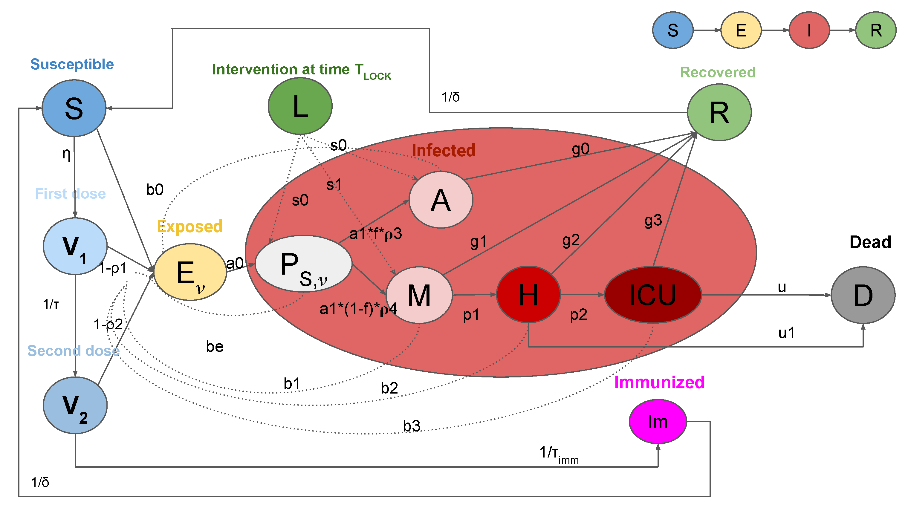
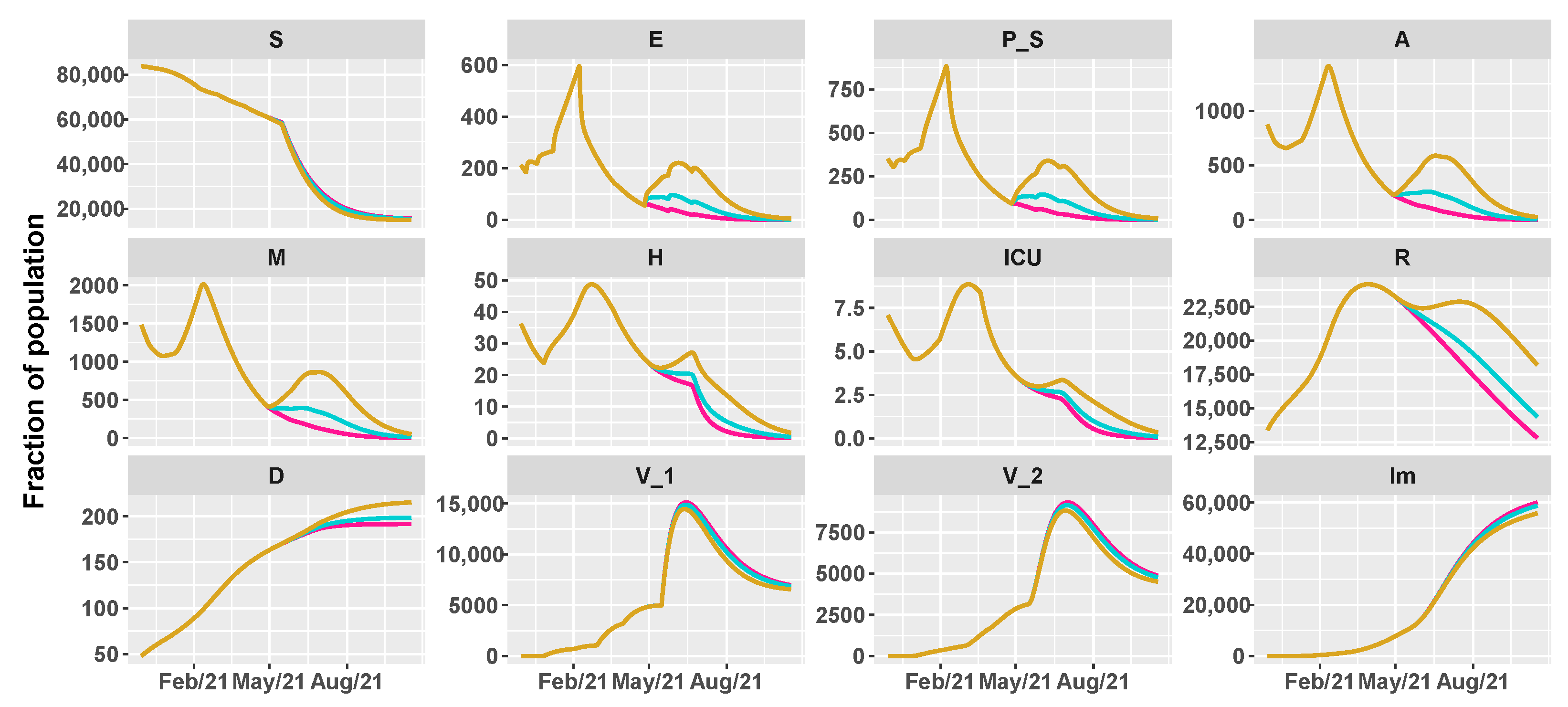
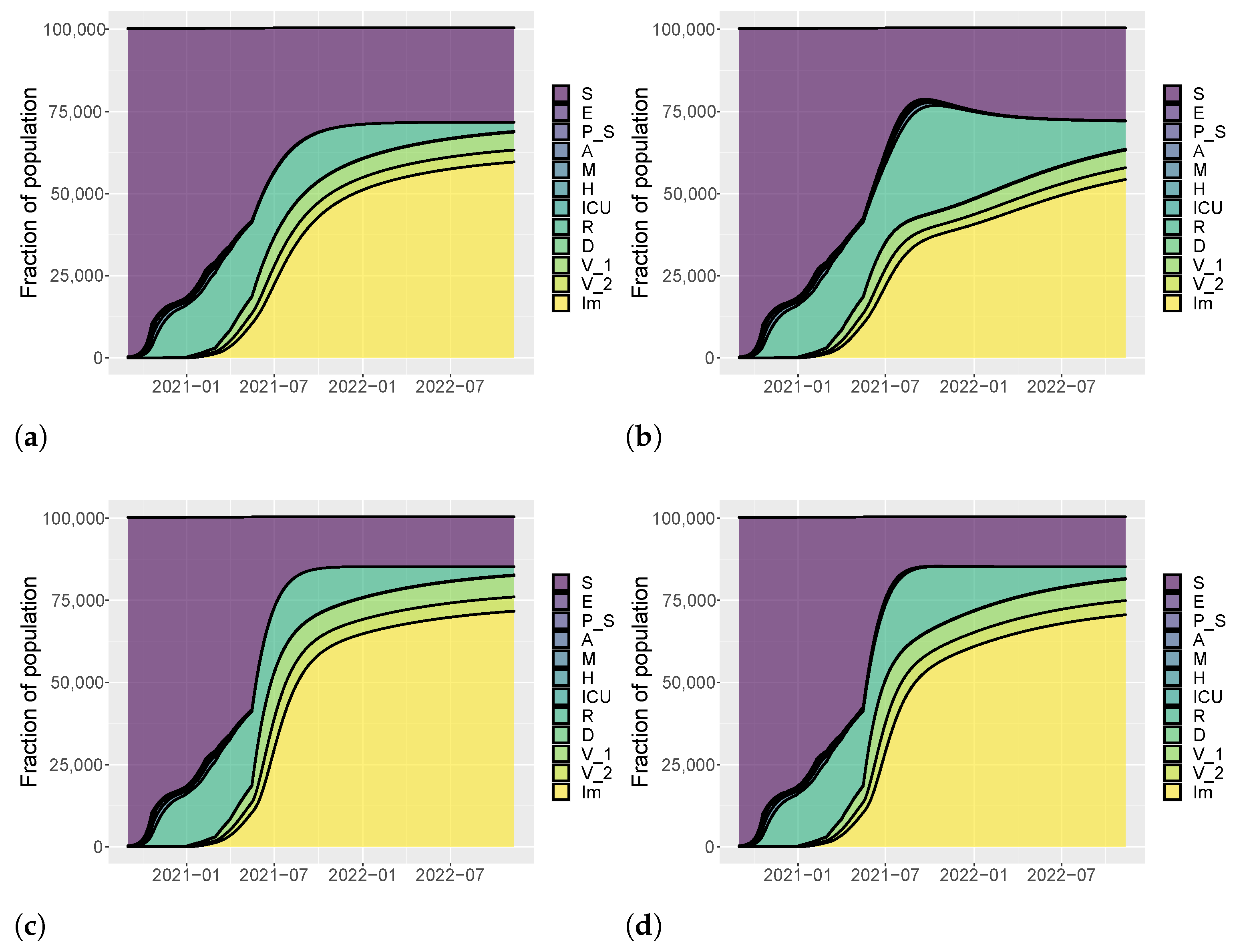
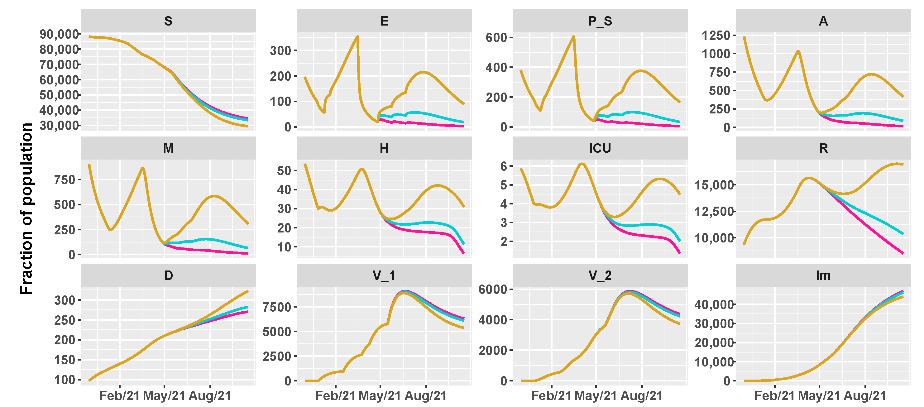
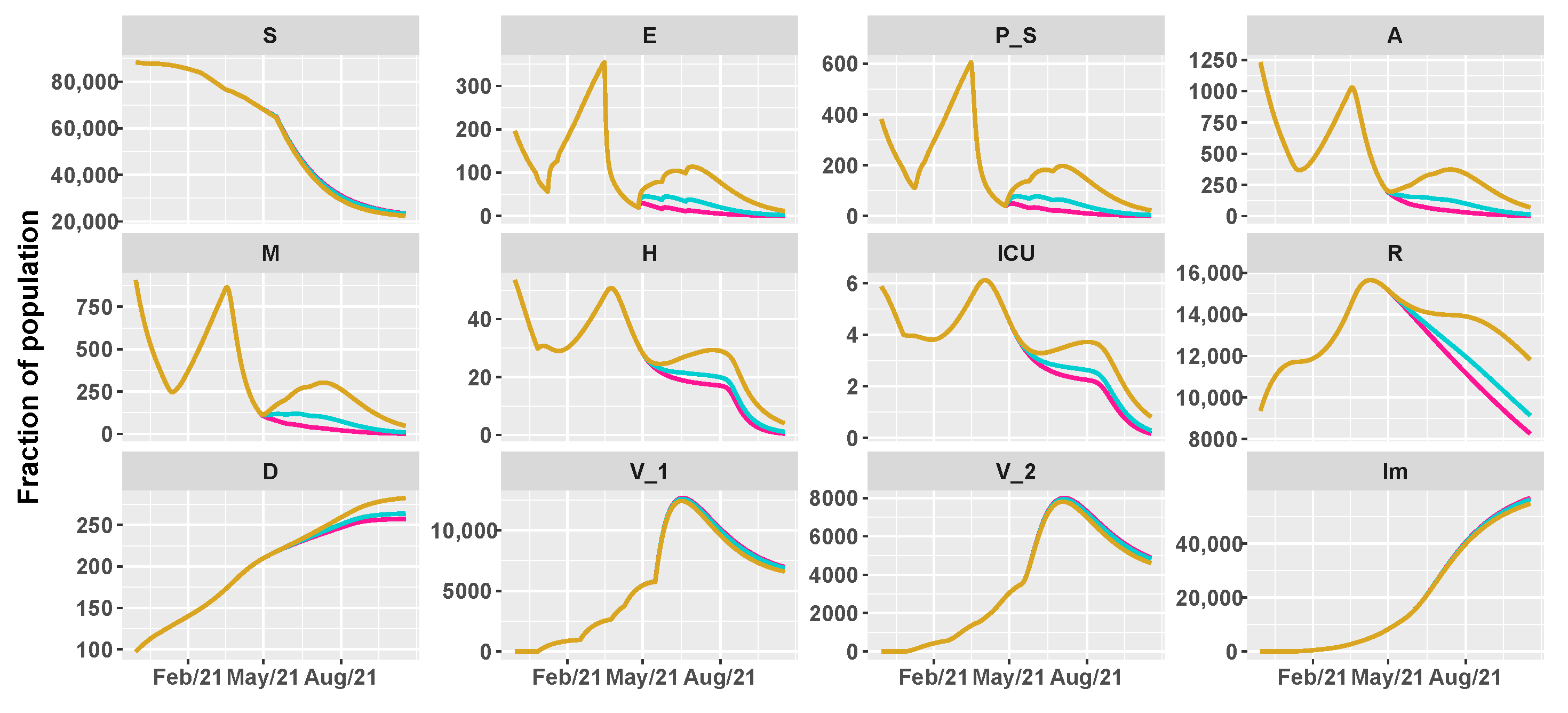
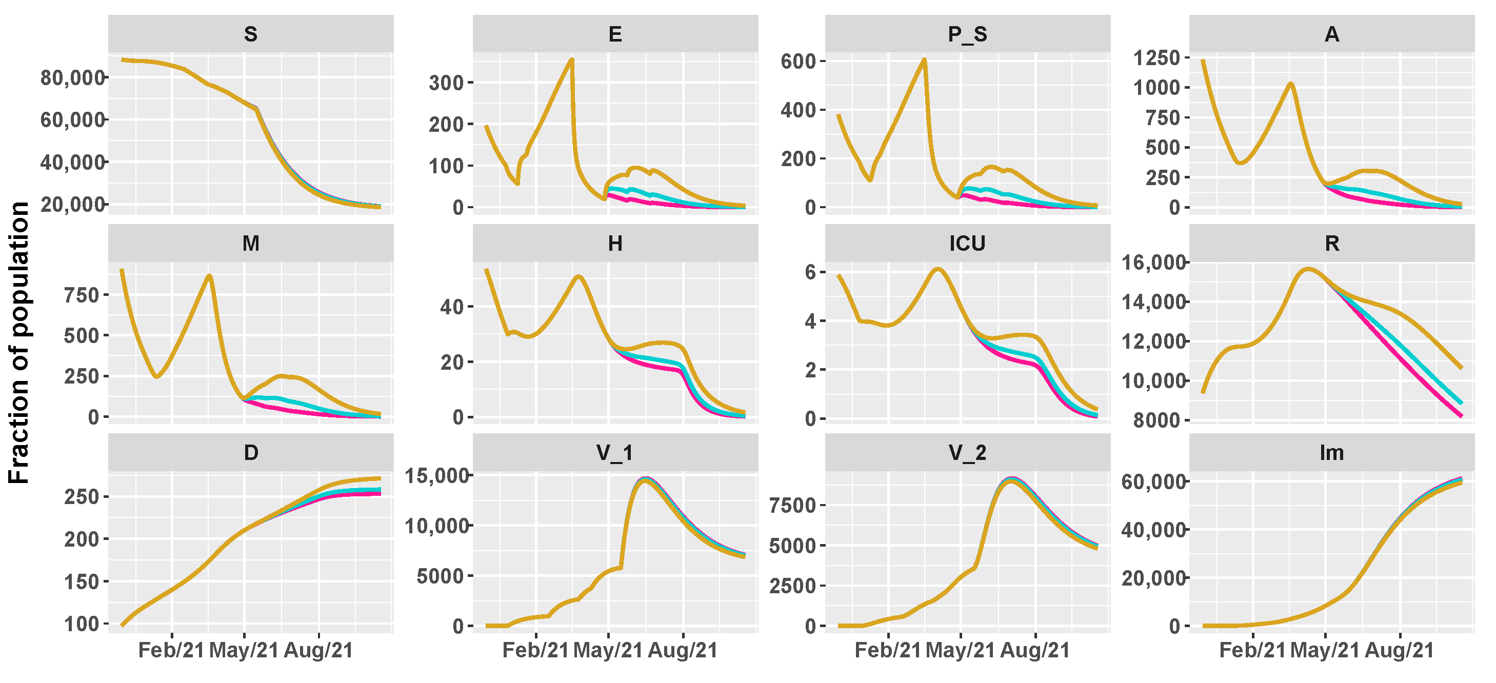
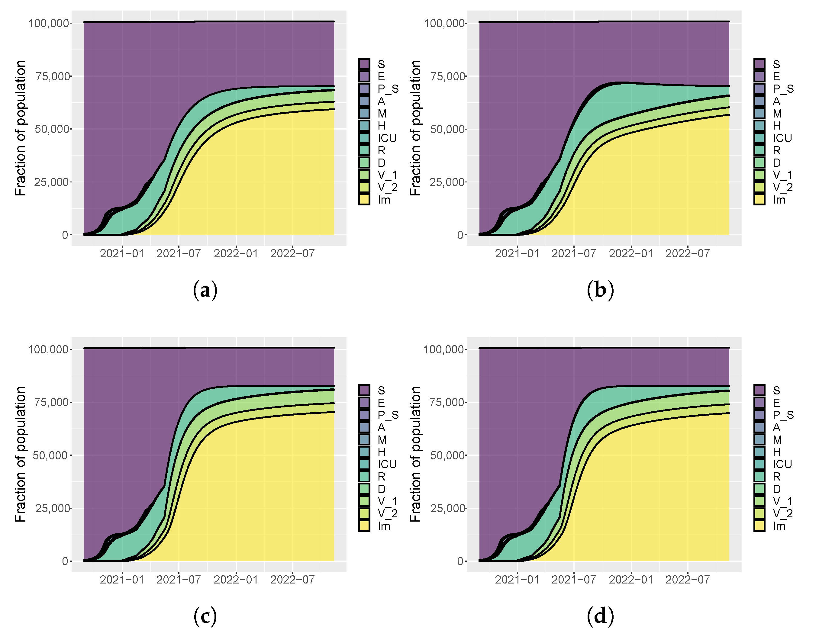
2.1. SEIRL-V Compartmental Model
- S: susceptible individuals,
- : exposed individuals, where denotes the numbers of vaccines doses received,
- : pre-symptomatic individuals, where denotes the numbers of vaccines doses received,
- A: asymptomatic individuals,
- M: people with mild infection,
- H: people in hospital with severe symptoms,
- : people with critical infection which requires ICU level care,
- R: recovered individuals,
- D: dead people,
- : people vaccinated with the first dose of vaccine,
- : people vaccinated with the second dose of vaccine,
- : immune individuals.
- with as the number of doses received. In more detail, , and .
- (1)
- (2)
- (3)
- (4)
- (5)
- (6)
- (7)
- (8)
- (9)
- (10)
- (11)
- ,
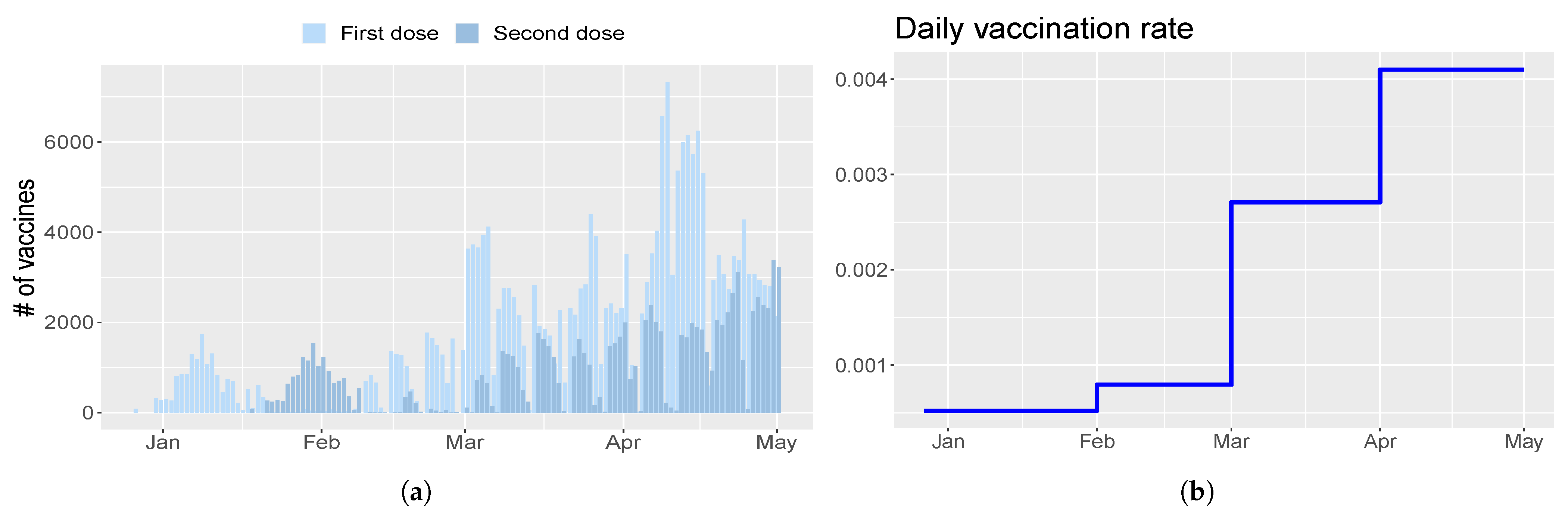
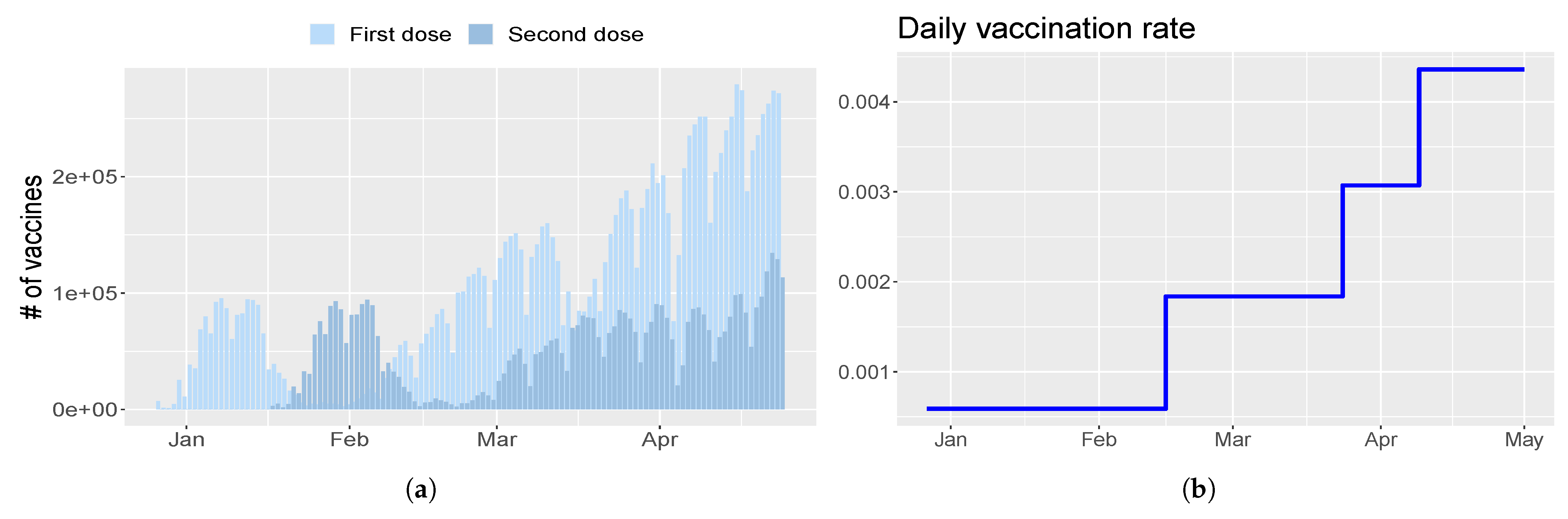
- parameter is the rate of injection of the first dose. It is modeled as a piecewise constant function;
- parameter is the time between the first and second dose of vaccine and it is set to 21 days [11];
- parameter is the number of days between the second dose and the acquired immunity and it is set to 14 days [11];
- parameter is the efficacy of the first shot of vaccine and it is set to 0.8 [27];
- parameter is the efficacy of the second shot of vaccine and it is set to 0.95 [11];
- parameter with is introduced to represent vaccine efficacy against disease. Thus, , and .
2.2. Data
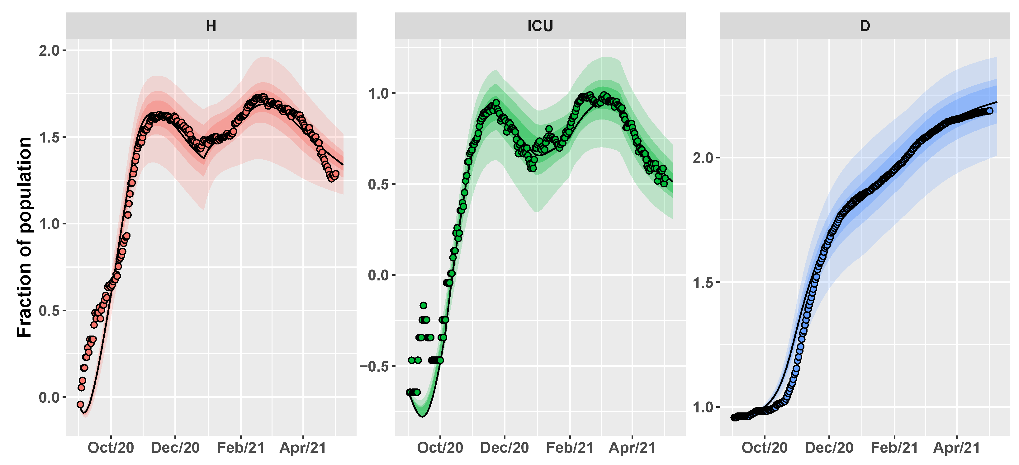
2.3. Conditional Robust Calibration (CRC) for Parameter Estimation
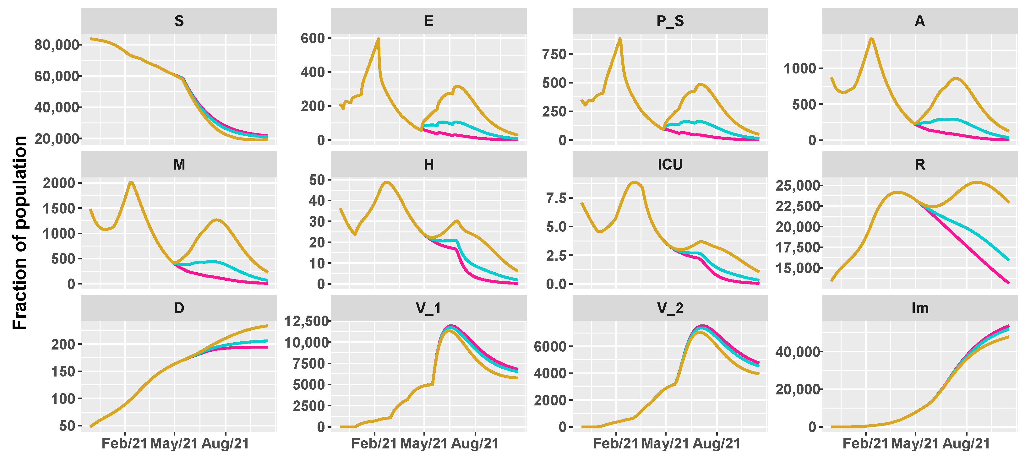
3. Results
3.1. Spread of Sars-CoV-2 Lineages in Umbria and Italy
3.2. Umbria Case Study
- (1)
- 14 September 2020 (), school reopening;
- (2)
- 19 October 2020 (), the Regional Government adopted some preventative measures such as remote teaching for part of the students, limited capacity of public transportation and closure of shopping malls during the weekend [37];
- (3)
- 11 November 2020 (), Umbria region is classified as “orange”, i.e., as a medium-risk contagion zone;
- (4)
- 6 December 2020 (), Umbria goes back to “yellow” zone, i.e., with moderate risk of virus spread;
- (5)
- 7 January 2021 (), school reopening and easing of some restrictions after the country-wide red area;
- (6)
- 8 February 2021 (), “red” area for the entire Province of Perugia, i.e., the highest level of restrictions, following an improvement in the contagion data and the identification of variants;
- (7)
- 22 March 2021 (), back to ’orange’ zone with reopening of schools for the youngest.
- from day 0 (1 September 2020) to day 35 (5 October 2020);
- from day 36 to day 83 (22 November 2020);
- from day 84 to day 152 (30 January 2021);
- from day 153 to day 200 (19 March 2021);
- from day 201 onward.
- 26 April 2021: reintroduction of the low-risk “yellow” zone;
- 24 May 2021: curfew extension, gym reopening and restaurants with indoor seating;
- 21 June 2021: curfew lifted and holiday season.
3.3. Italy Case Study
- (1)
- 14 September 2020 (), school reopening;
- (2)
- 6 November 2020 (), introduction of a three-tier color coded system of restrictive measures, based on the risk profile of each region;
- (3)
- 24 December 2020 (), country-wide lockdown for Christmas holidays;
- (4)
- 7 January 2021 (), school reopening and easing of some restrictions after the country-wide red area;
- (5)
- 15 March 2021 (), removal of ’yellow’ zone in the color-coded system, leaving only medium and high risk zones.
4. Discussion
5. Conclusions
Author Contributions
Funding
Institutional Review Board Statement
Informed Consent Statement
Data Availability Statement
Acknowledgments
Conflicts of Interest
Appendix A

| Parameter | 60th Percentile | 70th Percentile | 90th Percentile |
|---|---|---|---|
| [0.1483–0.1521] | [0.1462–0.154] | [0.1422–0.1581] | |
| [0.3084–0.3173] | [0.3032–0.3232] | [0.2895–0.3331] | |
| [0.2044–0.2377] | [0.1896–0.2609] | [0.1621–0.313] | |
| [0.3392–0.3589] | [0.3299–0.3673] | [0.31–0.3883] | |
| [0.0314–0.0365] | [0.0291–0.0387] | [0.0223–0.0441] | |
| [0.0158–0.0195] | [0.0142–0.0218] | [0.0114–0.0272] | |
| [0.0286–0.0342] | [0.0263–0.0379] | [0.0217–0.0461] | |
| [0.0166–0.0175] | [0.0161–0.018] | [0.0148–0.0192] | |
| [0.0044–0.0046] | [0.0043–0.0047] | [0.0041–0.0049] | |
| [0.0051–0.0054] | [0.005–0.0056] | [0.0047–0.0059] | |
| [0.0039–0.0041] | [0.0038–0.0042] | [.0036–0.0044] | |
| [0.0048–0.0051] | [0.0047–0.0052] | [0.0046–0.0054] | |
| [0.0028–0.003] | [0.0027–0.0031] | [0.0026–0.0034] | |
| [0.4738–0.4834] | [0.4684–0.4878] | [0.4567–0.4962] | |
| [4.4704–4.5473] | [4.429–4.591] | [4.3421–4.662] | |
| [15.8483–16.2392] | [15.63–16.4292] | [15.2157–16.809] | |
| [10.9094–11.3187] | [10.7329–11.4892] | [10.3026–11.844] | |
| [12.9659–13.3531] | [12.8103–13.5196] | [12.33–13.8242] | |
| [11.3651–11.5532] | [11.2718–11.6631] | [11.0916–11.8755] | |
| [28.5227–29.8384] | [27.5732–30.6969] | [25.865–32.129] | |
| [21.9761–22.7784] | [21.5211–23.2579] | [20.6255–24.3682] | |
| [0.5967–0.6039] | [0.5928–0.6085] | [0.5844–0.6163] | |
| n | [48.1783–51.8111] | [45.8733–53.8871] | [41.8768–57.764] |
| K | [–] | [–] | [–] |
| [1.0424–1.0614] | [1.0331–1.0727] | [1.0110–1.0911] | |
| [0.2722–0.2807] | [0.2663–0.2857] | [0.2562–0.2949] | |
| [0.263–0.2746] | [0.2578–0.2802] | [0.2456–0.2929] | |
| [0.4205–0.4297] | [0.4146–0.4346] | [0.4049–0.4447] | |
| [0.5608–0.5818] | [0.5506–0.5922] | [0.5307–0.6165] | |
| [0.2678–03279] | [0.2634–0.2839] | [0.2542–0.2944] | |
| [0.3181–0.3279] | [0.3126–0.334] | [0.3044–0.344] |
| Parameter | 60th Percentile | 70th Percentile | 90th Percentile |
|---|---|---|---|
| [0.1467–0.1559] | [0.1418–0.1609] | [0.1318–0.1721] | |
| [0.1933–0.2016] | [0.1901–0.2054] | [0.1833–0.214] | |
| [0.2686–0.2912] | [0.2587–0.3063] | [0.2393–0.3451] | |
| [0.1564–0.1711] | [0.1493–0.1792] | [0.1366–0.205] | |
| [0.0151–0.0189] | [0.0135–0.0208] | [0.0112–0.0261] | |
| [0.057–0.0608] | [0.0552–0.0627] | [0.0517–0.0677] | |
| [0.0157–0.0196] | [0.0141–0.0218] | [0.0112–0.0267] | |
| [0.0246–0.0258] | [0.024–0.0264] | [0.0221–0.0283] | |
| [0.0053–0.0054] | [0.0052–0.0055] | [0.0051–0.0057] | |
| [0.0066–0.0069] | [0.0064–0.007] | [0.0061–0.0073] | |
| [0.0033–0.0035] | [0.0033–0.0036] | [0.0031–0.0039] | |
| [0.0044–0.0045] | [0.0043–0.0046] | [0.0041–0.0049] | |
| [0.4622–0.4683] | [0.4592–0.4712] | [0.4529–0.4772] | |
| [5.1812–5.2188] | [5.16–5.2379] | [5.1188–5.2792] | |
| [9.3392–9.9241] | [9.0192–10.2157] | [8.366–10.7008] | |
| [14.6655–15.0305] | [14.4845–15.2173] | [14.1736–15.7103] | |
| [15.3648–15.5912] | [15.2701–15.7051] | [15.0902–15.8961] | |
| [12.3828–12.5781] | [12.2907–12.673] | [12.0992–12.8822] | |
| [34.7139–35.4889] | [34.3299–35.9058] | [33.4267–36.5895] | |
| [23.6944–24.3566] | [23.2392–24.8239] | [22.1059–25.5674] | |
| [0.615–0.6227] | [0.6114–0.6274] | [0.6033–0.6363] | |
| n | [50.9573–53.9461] | [49.4666–55.479] | [46.4324–58.8729] |
| K | [–] | [–] | [–] |
| [1.0205–1.0297] | [1.0153–1.0359] | [1.0055–1.0442] | |
| [0.3–0.3233] | [0.289–0.3369] | [0.2653–0.369] | |
| [0.242–0.2708] | [0.2305–0.2842] | [0.2099–03254] | |
| [0.6434–0.6667] | [0.6337–0.6829] | [0.612–0.7307] | |
| [0.1744–0.2092] | [0.1614–0.2262] | [0.1344–0.2704] |
References
- WHO. COVID-19 Dashboard; World Health Organization: Geneva, Switzerland, 2020; Available online: https://covid19.who.int/ (accessed on 15 June 2021).
- Vinceti, M.; Filippini, T.; Rothman, K.J.; Di Federico, S.; Orsini, N. SARS-CoV-2 infection incidence during the first and second COVID-19 waves in Italy. Environ. Res. 2021, 197, 111097. [Google Scholar] [CrossRef]
- Trasmissione Documento “Prevenzione e Risposta a Covid-19: Evoluzione Della Strategia e Pianificazione Nella Fase di Transizione Per il Periodo Autunno-Invernale. Available online: https://www.trovanorme.salute.gov.it/norme/renderNormsanPdf?anno=2020&codLeg=76597&parte=1%20&serie=null (accessed on 15 October 2020).
- Giordano, G.; Colaneri, M.; Di Filippo, A.; Blanchini, F.; Bolzern, P.; De Nicolao, G.; Sacchi, P.; Colaneri, P.; Bruno, R. Modeling vaccination rollouts, SARS-CoV-2 variants and the requirement for non-pharmaceutical interventions in Italy. Nat. Med. 2021, 27, 993–998. [Google Scholar] [CrossRef]
- Di Giallonardo, F.; Puglia, I.; Curini, V.; Cammà, C.; Mangone, I.; Calistri, P.; Cobbin, J.C.; Holmes, E.C.; Lorusso, A. Emergence and spread of SARS-CoV-2 lineages B. 1.1. 7 and P. 1 in Italy. Viruses 2021, 13, 794. [Google Scholar] [CrossRef]
- Davies, N.G.; Abbott, S.; Barnard, R.C.; Jarvis, C.I.; Kucharski, A.J.; Munday, J.D.; Pearson, C.A.; Russell, T.W.; Tully, D.C.; Washburne, A.D.; et al. Estimated transmissibility and impact of SARS-CoV-2 lineage B. 1.1. 7 in England. Science 2021, 372, 6538. [Google Scholar] [CrossRef]
- Faria, N.R.; Mellan, T.A.; Whittaker, C.; Claro, I.M.; Candido, D.d.S.; Mishra, S.; Crispim, M.A.; Sales, F.C.; Hawryluk, I.; McCrone, J.T.; et al. Genomics and epidemiology of the P. 1 SARS-CoV-2 lineage in Manaus, Brazil. Science 2021, 372, 815–821. [Google Scholar] [CrossRef]
- Prevalenza delle VOC (Variant of Concern) del virus SARS-CoV-2 in Italia: Blineage B.1.1.7, P.1 e B.1.351, e Altre Varianti (Variant of Interest, VOI) Tra Cui Lineage P.2 e Lineage B.1.525 (Indagine del 20 April 2021). Available online: https://www.iss.it/documents/20126/0/Relazione+tecnica+indagine+rapida+varianti+SARS-COV-2.pdf/f425e647-efdb-3f8c-2f86-87379d56ce8d?t=1620232350272 (accessed on 26 April 2021).
- COVID: Bolzano, Umbria Likely to Become Red Zones. Available online: https://www.ansa.it/english/news/politics/2021/02/19/covid-bolzano-umbria-likely-to-become-red-zones_b92c110b-a505-4100-a241-7ee2d459e8a0.html (accessed on 20 February 2021).
- Le, T.T.; Andreadakis, Z.; Kumar, A.; Román, R.G.; Tollefsen, S.; Saville, M.; Mayhew, S. The COVID-19 vaccine development landscape. Nat. Rev. Drug Discov. 2020, 19, 305–306. [Google Scholar] [CrossRef]
- Polack, F.P.; Thomas, S.J.; Kitchin, N.; Absalon, J.; Gurtman, A.; Lockhart, S.; Perez, J.L.; Pérez Marc, G.; Moreira, E.D.; Zerbini, C.; et al. Safety and efficacy of the BNT162b2 mRNA Covid-19 vaccine. N. Engl. J. Med. 2020, 383, 2603–2615. [Google Scholar] [CrossRef]
- Baden, L.R.; El Sahly, H.M.; Essink, B.; Kotloff, K.; Frey, S.; Novak, R.; Diemert, D.; Spector, S.A.; Rouphael, N.; Creech, C.B.; et al. Efficacy and safety of the mRNA-1273 SARS-CoV-2 vaccine. N. Engl. J. Med. 2021, 384, 403–416. [Google Scholar] [CrossRef] [PubMed]
- Voysey, M.; Clemens, S.A.C.; Madhi, S.A.; Weckx, L.Y.; Folegatti, P.M.; Aley, P.K.; Angus, B.; Baillie, V.L.; Barnabas, S.L.; Bhorat, Q.E.; et al. Single-dose administration and the influence of the timing of the booster dose on immunogenicity and efficacy of ChAdOx1 nCoV-19 (AZD1222) vaccine: A pooled analysis of four randomised trials. Lancet 2021, 397, 881–891. [Google Scholar] [CrossRef]
- Sadoff, J.; Gray, G.; Vandebosch, A.; Cárdenas, V.; Shukarev, G.; Grinsztejn, B.; Goepfert, P.A.; Truyers, C.; Fennema, H.; Spiessens, B.; et al. Safety and efficacy of single-dose Ad26. COV2. S vaccine against Covid-19. N. Engl. J. Med. 2021, 384, 2187–2201. [Google Scholar] [CrossRef] [PubMed]
- Piano Vaccini Anti Covid-19. Available online: https://www.salute.gov.it/portale/nuovocoronavirus/dettaglioContenutiNuovo-Coronavirus.jsp?lingua=italiano&id=5452&area=nuovoCoronavirus&menu=vuoto (accessed on 20 December 2020).
- Moore, S.; Hill, E.M.; Tildesley, M.J.; Dyson, L.; Keeling, M.J. Vaccination and non-pharmaceutical interventions for COVID-19: A mathematical modelling study. Lancet Infect. Dis. 2021, 21, 793–802. [Google Scholar] [CrossRef]
- Bubar, K.M.; Reinholt, K.; Kissler, S.M.; Lipsitch, M.; Cobey, S.; Grad, Y.H.; Larremore, D.B. Model-informed COVID-19 vaccine prioritization strategies by age and serostatus. Science 2021, 371, 916–921. [Google Scholar] [CrossRef] [PubMed]
- Saad-Roy, C.M.; Wagner, C.E.; Baker, R.E.; Morris, S.E.; Farrar, J.; Graham, A.L.; Levin, S.A.; Mina, M.J.; Metcalf, C.J.E.; Grenfell, B.T. Immune life history, vaccination, and the dynamics of SARS-CoV-2 over the next 5 years. Science 2020, 370, 811–818. [Google Scholar] [CrossRef] [PubMed]
- Antonini, C.; Calandrini, S.; Stracci, F.; Dario, C.; Bianconi, F. Mathematical Modeling and Robustness Analysis to Unravel COVID-19 Transmission Dynamics: The Italy Case. Biology 2020, 9, 394. [Google Scholar] [CrossRef] [PubMed]
- Bianconi, F.; Antonini, C.; Tomassoni, L.; Valigi, P. Robust calibration of high dimension nonlinear dynamical models for omics data: An application in cancer systems biology. IEEE Trans. Control Syst. Technol. 2018, 28, 196–207. [Google Scholar] [CrossRef]
- Bianconi, F.; Antonini, C.; Tomassoni, L.; Valigi, P. Application of conditional robust calibration to ordinary differential equations models in computational systems biology: A comparison of two sampling strategies. IET Syst. Biol. 2020, 14, 107–119. [Google Scholar] [CrossRef] [PubMed]
- Bianconi, F.; Tomassoni, L.; Antonini, C.; Valigi, P. A New Bayesian Methodology for Nonlinear Model Calibration in Computational Systems Biology. Front. Appl. Math. Stat. 2020, 6, 25. [Google Scholar] [CrossRef]
- López, L.; Rodo, X. A modified SEIR model to predict the COVID-19 outbreak in Spain and Italy: Simulating control scenarios and multi-scale epidemics. Results Phys. 2020, 21, 103746. [Google Scholar] [CrossRef]
- Covid-19 Opendata Vaccini, GitHub Repository. Available online: https://github.com/italia/covid19-opendata-vaccini (accessed on 1 June 2021).
- Dispinseri, S.; Secchi, M.; Pirillo, M.F.; Tolazzi, M.; Borghi, M.; Brigatti, C.; De Angelis, M.L.; Baratella, M.; Bazzigaluppi, E.; Venturi, G.; et al. Neutralizing antibody responses to SARS-CoV-2 in symptomatic COVID-19 is persistent and critical for survival. Nat. Commun. 2021, 12, 1–12. [Google Scholar] [CrossRef]
- Pfizer and BioNTech Initiate a Study as Part of Broad Development Plant o Evaluate Covid-19 Booster and New Variants. Available online: https://www.pfizer.com/news/press-release/press-release-detail/pfizer-and-biontech-initiate-study-part-broad-development (accessed on 27 February 2021).
- Thompson, M.G.; Burgess, J.L.; Naleway, A.L.; Tyner, H.L.; Yoon, S.K.; Meece, J.; Olsho, L.E.; Caban-Martinez, A.J.; Fowlkes, A.; Lutrick, K.; et al. Interim estimates of vaccine effectiveness of BNT162b2 and mRNA-1273 COVID-19 vaccines in preventing SARS-CoV-2 infection among health care personnel, first responders, and other essential and frontline workers—Eight US locations, December 2020–March 2021. Morb. Mortal. Wkly. Rep. 2021, 70, 495. [Google Scholar] [CrossRef]
- Task force COVID-19 del Dipartimento Malattie Infettive e Servizio di Informatica, Istituto Superiore di Sanità. Epidemia COVID-19. Aggiornamento Nazionale: 14 Luglio 2021. Available online: https://www.epicentro.iss.it/coronavirus/bollettino/Bollettino-sorveglianza-integrata-COVID-19_14-luglio-2021.pdf (accessed on 15 July 2021).
- Mateo-Urdiales, A.; Alegiani, S.S.; Fabiani, M.; Pezzotti, P.; Filia, A.; Massari, M.; Riccardo, F.; Tallon, M.; Proietti, V.; Del Manso, M.; et al. Risk of SARS-CoV-2 infection and subsequent hospital admission and death at different time intervals since first dose of COVID-19 vaccine administration, Italy, 27 December 2020 to mid-April 2021. Eurosurveillance 2021, 26, 2100507. [Google Scholar] [CrossRef]
- Nguyen, L.K.; Kulasiri, D. On the functional diversity of dynamical behaviour in genetic and metabolic feedback systems. BMC Syst. Biol. 2009, 3, 51. [Google Scholar] [CrossRef] [Green Version]
- Fosu, G.O.; Akweittey, E.; Adu-Sackey, A. Next-generation matrices and basic reproductive numbers for all phases of the Coronavirus disease. Open J. Math. Sci. 2020, 4, 261–272. [Google Scholar] [CrossRef]
- Dipartimento Protezione Civile, GitHub Repository. Available online: https://github.com/pcm-dpc/COVID-19 (accessed on 2 May 2021).
- SARS-CoV-2 Variant Classifications and Definitions. Available online: https://www.cdc.gov/coronavirus/2019-ncov/cases-updates/variant-surveillance/variant-info.html#Concern (accessed on 15 May 2021).
- Pearson, C.A.; Russell, T.W.; Davies, N.; Kucharski, A.J.; CMMID COVID-19 working group; Edmunds, W.J.; Eggo, R.M. Estimates of Severity and Transmissibility of Novel South Africa SARS-CoV-2 Variant 501Y. V2. Available online: https://cmmid.github.io/topics/covid19/sa-novel-variant.html (accessed on 1 May 2021).
- Prevalenza Della Variante VOC 202012/01, Lineage B.1.1.7 in Italia, Studio di Prevalenza 4–5 Febbraio 2021. Available online: https://www.iss.it/documents/20126/0/Relazione+tecnica+prima+indagine+flash+VOC+UK+12.2.2021_rev+finale.pdf/636b3651-a358-468e-24d5-65364a004994?t=1613400983576 (accessed on 10 February 2021).
- Prevalenza Delle Varianti VOC 202012/01 (Lineage B.1.1.7), P.1, e 501.V2 (Lineage B.1.351) in Italia Indagine del 18 Febbraio 2021. Available online: https://www.iss.it/documents/20126/0/Relazione+tecnica+terza+indagine+flash+per+le+varianti+del+virus+SARS-CoV-2+%282%29.pdf/a03f33e6-d775-9ab0-b0ce-9cdd289c711d?t=1614707205598 (accessed on 20 February 2021).
- Ordinanza della Presidente Della Giunta Regionale, 19 Ottobre 2020, n. 65. Available online: https://www.regione.umbria.it/documents/18/24917656/ORDINANZA_65.pdf/80514ae4-6ae5-43f0-a0d7-43e23dae6194 (accessed on 20 October 2020).
- Riaperture Italia, il Calendario del Governo. Available online: https://www.adnkronos.com/riaperture-italia-il-calendario-del-governo_4GbnBUMmxOnrDY2YEKt5Jv (accessed on 17 May 2021).
- Anderson, R.M.; Vegvari, C.; Truscott, J.; Collyer, B.S. Challenges in creating herd immunity to SARS-CoV-2 infection by mass vaccination. Lancet 2020, 396, 1614–1616. [Google Scholar] [CrossRef]
- D’Souza, G.; Dowdy, D. What’s herd immunity and how can we achieve it with COVID-19. Johns Hopkins Sch. Public Health Expert Insights. 2020, 10. Available online: https://www.jhsph.edu/covid-19/articles/achieving-herd-immunity-with-covid19.html (accessed on 1 June 2021).
- Certificazioni Verdi Covid-19. Available online: https://www.salute.gov.it/portale/nuovocoronavirus/dettaglioFaqNuovo-Coronavirus.jsp?lingua=italiano&id=264 (accessed on 1 June 2021).
- COVID-19: What You Have to Know about It. Available online: https://www.inmp.it/eng/CoViD-19-what-you-have-to-know-about-it/Covid-19-Red-zone (accessed on 15 January 2021).
- Epidemia COVID-19 Aggiornamento Nazionale 27 Ottobre 2020—Ore 11:00. Available online: https://www.epicentro.iss.it/coronavirus/bollettino/Bollettino-sorveglianza-integrata-COVID-19_27-ottobre-2020.pdf (accessed on 31 October 2020).
- Epidemia COVID-19 Aggiornamento Nazionale 18 Novembre 2020—Ore 11:00. Available online: https://www.epicentro.iss.it/coronavirus/bollettino/Bollettino-sorveglianza-integrata-COVID-19_18-novembre-2020.pdf (accessed on 21 November 2020).
- Ledford, H. COVID reinfections are unusual-but could still help the virus to spread. Nature 2021. [Google Scholar] [CrossRef]
- Britton, T.; Ball, F.; Trapman, P. A mathematical model reveals the influence of population heterogeneity on herd immunity to SARS-CoV-2. Science 2020, 369, 846–849. [Google Scholar] [CrossRef]
- Fontanet, A.; Cauchemez, S. COVID-19 herd immunity: Where are we? Nat. Rev. Immunol. 2020, 20, 583–584. [Google Scholar] [CrossRef]


| Parameter | Prior | Umbria | Italy |
|---|---|---|---|
| log-U(0.01,1) | 0.1442 | 0.1342 | |
| log-U(0.01,1) | 0.3178 | 0.2109 | |
| log-U(0.01,1) | 0.2172 | 0.2512 | |
| log-U(0.01,1) | 0.3672 | 0.19 | |
| log-U(0.001,1) | 0.0269 | 0.0120 | |
| log-U(0.001,1) | 0.0119 | 0.0516 | |
| log-U(0.001,1) | 0.0260 | 0.0145 | |
| log-U(0.01,0.08) | 0.0182 | 0.0253 | |
| log-U(0.001,0.02) | 0.0041 | 0.005 | |
| log-U(0.001,0.02) | 0.0055 | 0.007 | |
| log-U(0.001,0.02) | 0.0045 | 0.0035 | |
| log-U(0.001,0.02) | 0.0053 | 0.0048 | |
| log-U(0.001,0.02) | 0.0033 | - | |
| U(0.2,0.7) | 0.488 | 0.4618 | |
| U(4,6) | 4.6389 | 5.2668 | |
| U(5,30) | 15.6157 | 9.8982 | |
| U(5,20) | 10.7014 | 14.5149 | |
| U(4,30) | 13.2214 | 15.6204 | |
| U(4,30) | 11.1608 | 12.6742 | |
| U(10,90) | 31.0621 | 34.7989 | |
| U(10,90) | 22.2085 | 25.3705 | |
| log-U(0.5,0.9) | 0.6075 | 0.637 | |
| n | U(1,100) | 47.1727 | 47.1717 |
| K | U(1,) | ||
| log-U(0.4,1.5) | 1.0729 | 1.0409 | |
| log-U(0.1,0.9) | 0.2705 | 0.3095 | |
| log-U(0.1,0.9) | 0.2815 | 0.2634 | |
| log-U(0.4,1.5) | 0.432 | 0.6842 | |
| log-U(0.4,1.5) | 0.5805 | 0.1837 | |
| log-U(0.1,0.9) | 0.2952 | - | |
| log-U(0.1,0.9) | 0.3077 | - |
| Vaccination Rate | |||||||
|---|---|---|---|---|---|---|---|
| Umbria | Italy | ||||||
| Intervention | [0.4–0.6–0.8] | Low/Low | Low/Medium | Low/High | Low/Low | Low/Medium | Low/High |
| [0.6–0.8–1] | Medium/Low | Medium/Medium | Medium/High | Medium/Low | Medium/Medium | Medium/High | |
| [0.8–1–1.2] | High/Low | High/Medium | High/High | High/Low | High/Medium | High/High | |
Publisher’s Note: MDPI stays neutral with regard to jurisdictional claims in published maps and institutional affiliations. |
© 2021 by the authors. Licensee MDPI, Basel, Switzerland. This article is an open access article distributed under the terms and conditions of the Creative Commons Attribution (CC BY) license (https://creativecommons.org/licenses/by/4.0/).
Share and Cite
Antonini, C.; Calandrini, S.; Bianconi, F. A Modeling Study on Vaccination and Spread of SARS-CoV-2 Variants in Italy. Vaccines 2021, 9, 915. https://doi.org/10.3390/vaccines9080915
Antonini C, Calandrini S, Bianconi F. A Modeling Study on Vaccination and Spread of SARS-CoV-2 Variants in Italy. Vaccines. 2021; 9(8):915. https://doi.org/10.3390/vaccines9080915
Chicago/Turabian StyleAntonini, Chiara, Sara Calandrini, and Fortunato Bianconi. 2021. "A Modeling Study on Vaccination and Spread of SARS-CoV-2 Variants in Italy" Vaccines 9, no. 8: 915. https://doi.org/10.3390/vaccines9080915