Article

An Optimal Control Model to Understand the Potential Impact of the New Vaccine and Transmission-Blocking Drugs for Malaria: A Case Study in Papua and West Papua, Indonesia

by
Bevina D. Handari
1,
Rossi A. Ramadhani
1,
Chidozie W. Chukwu
2,
Sarbaz H. A. Khoshnaw
3 and
Dipo Aldila
1,*
1
Department of Mathematics, Universitas Indonesia, Depok 16424, Indonesia
2
Division of Infectious Diseases and Global Public Health, University of California, San Diego, CA 94720, USA
3
Department of Mathematics, University of Raparin, Ranya 46012, Kurdistan Region, Iraq
*
Author to whom correspondence should be addressed.
Vaccines 2022, 10(8), 1174; https://doi.org/10.3390/vaccines10081174
Submission received: 30 May 2022 / Revised: 19 July 2022 / Accepted: 19 July 2022 / Published: 24 July 2022
(This article belongs to the Special Issue Dynamic Models in Viral Immunology)

Abstract

:
Malaria is one of the major causes of a high death rate due to infectious diseases every year. Despite attempts to eradicate the disease, results have not been very successful. New vaccines and other treatments are being constantly developed to seek optimal ways to prevent malaria outbreaks. In this article, we formulate and analyze an optimal control model of malaria incorporating the new pre-erythrocytic vaccine and transmission-blocking treatment. Sufficient conditions to guarantee local stability of the malaria-free equilibrium were derived based on the controlled reproduction number condition. Using the non-linear least square fitting method, we fitted the incidence data from the province of Papua and West Papua in Indonesia to estimate the model parameter values. The optimal control characterization and optimality conditions were derived by applying the Pontryagin Maximum Principle, and numerical simulations were also presented. Simulation results show that both the pre-erythrocytic vaccine and transmission-blocking treatment significantly reduce the spread of malaria. Accordingly, a high doses of pre-erythrocytic vaccine is needed if the number of infected individuals is relatively small, while transmission blocking is required if the number of infected individuals is relatively large. These results suggest that a large-scale implementation of both strategies is vital as the world continues with the effort to eradicate malaria, especially in endemic regions across the globe.

1. Introduction

The primary cause of any infectious disease is the spread of pathogens such as bacteria, viruses, parasites, or fungus. Some of these diseases can spread from person to person, either through direct or indirect contact. A disease that spreads in the human population with an intermediate vector is called a vector-borne disease. According to the world health organization (WHO) [1], vector-borne infection contributes to over 17% of total infectious disease cases worldwide, with an estimated 700,000 deaths annually. Malaria is a vector-borne disease that threatens millions of people every year. Most of the cases come from Africa, southeast Asia, the eastern Mediterranean, and West Pacific [2]. Globally, there were over 600,000 deaths reported out of over 240 million detected cases in 2020. In Indonesia, over 74% of all detected cases are from the provinces of Papua and West Papua [3].
Malaria spreads through the bite of female Anopheles mosquitoes from previously infected individuals with Plasmodium (P). The five types of Plasmodium that cause malaria are P. falciparum, P. vivax, P. malariae, P. ovale, and P. knowlesi [4]. Globally, among all these types of Plasmodium, P. falciparum is primarily commonly found in African countries, while P.vivax exists in other parts of the world (that is, outside Africa) [5]. Several forms of intervention to control the spread of malaria have been introduced for many years worldwide. Most forms of intervention aim to control the population of mosquitoes in the field, such as with the use of fumigation, larvacide, or insecticide-treated bed nets [6]. Other than vector control, malaria prevention also focuses on developing a new vaccine to prevent new infections in the human population. Based on the life cycle of Plasmodium in the human body, the malaria vaccine is divided into three types, namely pre-erythrocytic vaccine, blood-stage vaccine, and transmission-blocking vaccine [7]. The pre-erythrocytic vaccine was designed to eliminate sporozoites immediately after mosquitoes inject Plasmodium into the human body. It will also block the Plasmodium from going to the human liver. According to the WHO report [5], RTS, S/AS01 is one type of pre-erythrocytic vaccine that is recommended by WHO to kill P. falciparum in children population. The blood-stage vaccine is introduced to target the asexual stage of Plasmodium (merozoites) in human red blood cells. On the other hand, the transmission-blocking vaccine is given such that further infection can be avoided [8]. Other than the transmission-blocking vaccine, a type of transmission-blocking drug has been used to eliminate the sexual stages of Plasmodium in human or mosquito bodies.
Mathematical models have been used for many years to understand the mechanisms of malaria transmission, since such model approaches can be used to give a visual interpretation of any possible intervention that can be implemented in the field to control malaria transmission. These approaches provide a scientific background before a final decision from the government should be taken. From the early work by Ross [9] in 1911, many mathematical models were introduced by authors to help a better understanding of malaria transmission. Macdonald in 1957 [10] used his model to estimate the infection and recovery rates of malaria. He found that reducing the number of mosquitoes in an endemic area is an inefficient malaria control strategy. In the early 1980s–1990s, Anderson and May [11] and Aron and May [12] constructed their malaria model based on the assumption that immunity to malaria is independent of the duration of exposure. Okosun et al., in [13], concluded from their mathematical model that a combination between insecticides and transmission-blocking treatment is the most cost-effective interventions to control malaria. An optimal vaccination and bed net mathematical model have been introduced by Prosper et al. in [14]. Their analytical result reveals that increasing the case detection strategy may reduce the chance of backward bifurcation phenomena in their model. An analysis of the potential impact of pre-erythrocytic vaccine from clinical data was discussed by the author in [15]. Similar to Prosper et al. in [14], Woldegerima et al. in [16] also found a possible backward bifurcation from their model on the impact of transmission-blocking drugs. Their model projects an approximately 82% death rate is reduced by 2035 if 35% of the population in Sub-Saharan Africa receives a transmission-blocking drug with an efficacy of 95%. Kuddus and Rahman in [17] analyze the dynamics of malaria using incidence data in Bangladesh from 2001 to 2014. They found that as infection rate has the greatest impact on the basic reproduction number compared to other model parameters, it is important to reduce this infection rate, such as using insecticide-treated bed nets, spraying insecticides, clearing stagnant water, etc. In a more recent mathematical model, authors include more recent facts on malaria transmission such as the effect of vector-bias [18], asymptotic carriers [19], age-structured [20], competitive strains [21], seasonal factor [22,23], and coinfection of malaria with COVID-19 [24]. Furthermore, intervention models also have been widely introduced by authors, such as the use of fumigation [25], insecticide-treated bed nets [26], and vaccines with waning immunity [27], or transmission-blocking vaccines [28].
The authors in [29] concluded that a better understanding of Plasmodium development in the pre-erythrocytic stage could lead to the discovery of new antigenic targets for enhanced immunization strategies. These findings may aid in the development of new malaria immunization techniques that are more successful and useful. In 2015, GlaxoSmithKline’s (GSK’s) R T S ,   S / A S 01 pre-erythrocytic vaccine received a positive scientific response on the quality of this vaccine in combating malaria transmission [30]. Based on the above description, we consider it essential to see the potential impact of the pre-erythrocytic vaccine ( R T S ,   S / A S 01 ) and transmission-blocking drug as a combination of control to reduce the spread of malaria using a mathematical model approach.
Our model divided the susceptible population based on a condition, whether they use a pre-erythrocytic vaccine or not. Furthermore, we also consider the possibility that the transmission-blocking drug cannot kill all Plasmodium in either the sexual or asexual stage in the human body. We used incidence data from Papua and West Papua to calibrate our model by determining the best-fit parameter on our model. Sensitivity analysis on the basic reproduction number and the numerical simulation on the dynamics of each compartment are also conducted to see the impact of pre-erythrocytic vaccine and transmission-blocking drugs in the malaria control strategy. An optimal control model is then analyzed to determine the best possible scenario for combining pre-erythrocytic vaccine and transmission-blocking drugs. The novelty of our model lies in the originality of the model, where we discuss the potential impact of the pre-erythrocytic vaccine. Furthermore, we also use incidence data from two provinces in Indonesia, namely Papua and West Papua, to calibrate our model parameters. These incidence data have never been used in any malaria mathematical model.
The organization of this paper is as follows. In Section 2, we construct our model based on our assumptions, and estimate the parameter values on our model by fitting the output of our model with incidence data in Papua and West Papua. Dynamical analysis regarded the positiveness of the solution of our model, the existence and stability of equilibrium points, and the controlled reproduction number discussed in Section 3. Sensitivity analysis is given in Section 4. Existence of optimal solution and the characterization of the optimal control problem are given in Section 5 and Section 6, respectively. Finally, some conclusions are given in Section 7.

2. The Model and Parameter Estimation Result
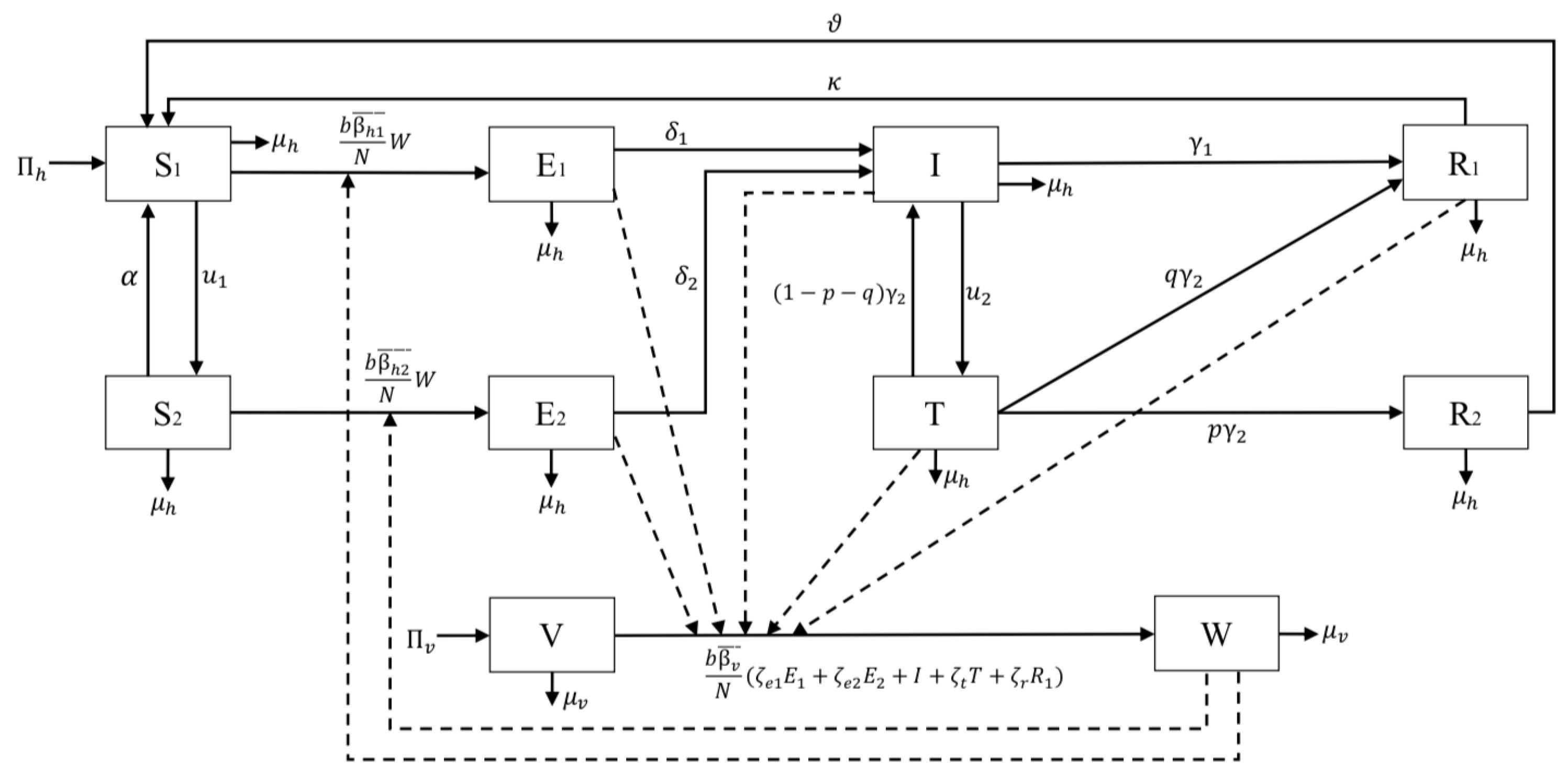
2.1. The Model

Based on the malaria status in the human and mosquitoes population, we divided the total human population (denoted by N) into eight compartments as follows:
1.
Susceptible without vaccine ( S 1 ) consists of a group of individuals susceptible to malaria who have not received a pre-erythrocytic vaccine yet.
2.
Susceptible with a vaccine ( S 2 ) consists of a group of individuals who are also susceptible to malaria but have already received a pre-erythrocytic vaccine.
3.
Exposed without vaccine ( E 1 ) consists of a group of newly infected individuals from S 1 who have not yet gotten the pre-erythrocytic vaccine. We assume that individuals in this compartment are in the leaver stage. Hence, although these individuals do not show any symptoms yet, we assume that they can transmit Plasmodium to susceptible mosquitoes.
4.
Exposed with vaccine ( E 2 ) consists of a group of newly infected individuals from S 2 . Although these individuals have already gotten vaccinated, the description is still the same with E 1 .
5.
Infected ( I ) consists of a group of individuals who have already gotten infected by malaria and show their symptoms.
6.
Infected individuals undergo transmission-blocking treatment ( T ) , defined as a group of individuals who already get infected, show symptoms, but get a transmission-blocking treatment. We assume that this treatment can kill the sexual Plasmodium (gametocytes).
7.
Recovered but carrier ( R 1 ) consists of individuals who recovered from malaria (do not show symptoms anymore) and have a temporal immunity but still have asexual Plasmodium inside their bodies. Hence, this group of individuals can still transmit Plasmodium to the mosquito.
8.
Fully recovered ( R 2 ) consists of a group of individuals who recovered from malaria and succeeded in the transmission-blocking treatment process. Hence, unlike in R 1 , individuals in R 2 lack sexual and asexual Plasmodium in their blood. Therefore, R 2 compartment does not transmit malaria anymore.
On the other hand, we only divide the mosquitoes population (denoted by M) into two compartments, namely the susceptible and infected mosquitoes, denoted by V and W, respectively.
We use the following assumptions to construct the model:
1.
The rate of new individuals only came from newborns with a constant rate of Π h . We ignore migration from our model.
2.
Vertical transmission is neglected [31].
3.
The infected individuals in E 1 , E 2 , I , T , and R 1 are capable to transmit Plasmodium to mosquitoes with a constant rate β v .
4.
The pre-erythrocytic vaccine is given to S 1 individuals with a constant rate u 1 to give temporal protection from mosquito bites that can lead to malaria infection. Hence, we assume that the transmission rate of S 2 is less than S 1 ( β h 2 < β h 1 ) .
5.
The pre-erythrocytic vaccine is not for a lifetime. Hence, after a period of α 1 , individuals in S 2 will return to S 1 .
6.
The transmission-blocking treatment is given to individuals in I with a constant rate u 2 to cure malaria and wipe out sexual and asexual Plasmodium from their blood.
7.
The transmission-blocking treatment is not always successful in curing infected individuals.
8.
The description of all parameters is given in Table 1 and assumed to be nonnegative.
The construction of the model is based on the transmission diagram in Figure 1. All newborns in human and mosquito populations are assumed to be susceptible, with a rate of Π h and Π v , respectively. On the other hand, we assume that each compartment has a natural death rate of μ h and μ v for human and mosquito populations, respectively. According to [32,33], the total inhabitants in Papua and West papua are 3,453,430 and 981,822, respectively.
Our main purpose is to understand the potential impact of the pre-erythrocytic vaccine on reducing the possible transmission of malaria in the human population. This vaccine was designed to clean the sporozoite from the human body right after the mosquito injects the Plasmodium into the human body and block the sporozoites’ invasion of the human liver cell. Hence, we include the rate of this pre-erythrocytic with a constant rate of u 1 to the susceptible population ( S 1 ) . This vaccine is not for a lifetime [37]. Hence, after a certain period of time, individuals in S 2 will return to S 1 . We denote this dropout rate with α . The transmission of malaria comes from the bite of infected mosquitoes to susceptible humans. We assume that the successful transmission rates of S 1 and S 2 are denoted by β h 1 ¯ and β h 2 ¯ , respectively. Let b be the average number of mosquitoes bite per month, then b β h 1 ¯ and b β h 2 ¯ are the averages of possible success transmission in S 1 and S 2 each month due to the bite of one infected mosquitoes, respectively. We use a ratio-dependent function to model our infection term. Therefore, the number of total infections in S 1 is given by b β h 1 ¯ W S 1 N . We assume that the total human population is constant. Therefore, b β h 1 ¯ N is constant, and we denote it by β h 1 . Therefore, we have that the total number of new infections in the human population from the S 1 compartment is given by β h 1 S 1 W . Using the same approach, the number of new infections in S 2 is given by β h 2 S 2 W . Exposed individuals without vaccine ( E 1 ) and with vaccine ( E 2 ) move to Infected class ( I ) due to progression rate δ 1 and δ 2 , respectively. Note that due to the effect of pre-erythrocytic vaccine that can suppress invasion of sporozoites in hepatocytes [8], we have δ 2 < δ 1 . Without treatment, we assume that infected individual I can recover with a constant rate γ 1 .
Another essential factor that is considered in this article is the use of transmission-blocking treatment for infected individuals I. We assume that individuals in I get a treatment with a constant rate u 2 , which will transfer them into compartment T. This treatment is given in a duration of γ 2 1 . Hence, after a period of γ 2 1 , the result of this treatment should be evaluated. If the treatment successfully kills all sexual and asexual parasites, then they are transferred to the compartment of R 2 with a rate of p γ 2 . If the treatment only partially succeeds where only sexual parasites could be eliminated but not the asexual parasites, these individuals will go to R 1 with a rate of q γ 2 . Finally, if the treatment fails, then individuals in T go back to I with a rate of ( 1 p q ) γ 2 . We assume that individuals in R 1 still could infect mosquitoes, but they are immune to the symptoms of malaria. Further, we also assume that they have a temporal immunity of κ 1 . On the other hand, individuals in R 2 cannot transfer Plasmodium to mosquitoes and have a temporal immunity of ϑ 1 .
Unlike the human population, the modeling of the mosquito population is not as complex. It only involves newborn Π v , natural death rate μ v , and infection. We assume that susceptible mosquitoes will get infected if they bite infected individuals in compartments E 1 , E 2 , I , T , and R 1 . Since the status of parasites in each mentioned compartment is in different stages, we assume the transmission rate for the mosquitoes are different based on their parasites status. Gametocytes are sexual forms of parasites produced by blood-stage merozoites. However, for P. vivax, gametocytes can be produced by liver stage merozoites [39]. Therefore, humans still in the pre-erythrocyte stage can also transmit susceptible mosquitoes. Exposed humans who received the pre-erythrocytic vaccine ( E 1 ) will have fewer parasites in the liver, so the likelihood of liver-stage merozoites producing gametocytes will be less than that of exposed unvaccinated humans ( E 2 ) . In addition, according to [39], gametocytes can still be found in peripheral blood after several weeks of asexual parasite infection being cleared, so recovered humans ( R 1 ) can still transmit susceptible mosquitoes. Humans in treatment can transmit susceptible mosquitoes because humans in treatment ( T ) are people who are still infected or have not been fully treated. Hence, the transmission rate of E 1 , E 2 , R , T to susceptible mosquitoes are given by ζ e 2 β v ¯ , ζ e 1 β v ¯ , ζ r β v ¯ , and ζ t β v ¯ , respectively. Note that ζ e 1 , ζ e 2 , ζ r , and ζ t are the correction parameters due to parasites’ stage in human body, and satisfies the following inequality:
0 < ζ e 2 < ζ e 1 < ζ r < ζ t < 1 .
Therefore, the total of new infection in mosquitoes population is given by
β v ζ e 1 E 1 + ζ e 2 E 2 + I + ζ r R + ζ t T V ,
where β v = b β v ¯ N . From all mentioned parameters above, we must understand that some parameters, especially in the mosquito population, might depend on time or other factors such as weather. For example, mosquitoes are more active when the temperature is low, which means that mosquitoes will be more active in biting humans when the temperature is relatively low [40]. Based on this explanation, all parameter values in our model as in Table 1 are average values.
In many mathematical models for disease control, an optimal control approach is commonly used by many authors to understand the behavior of each intervention as a time-dependent variable under a specific budget limitation problem [41,42,43]. Our proposed model has two different forms of intervention: the pre-erythrocytic vaccine and transmission-blocking treatment, denoted by u 1 and u 2 , respectively. In this article, these two forms of intervention will be treated as a time-dependent variable to pursue the best strategy to suppress the spread of malaria. Hence, we have u 1 = u 1 ( t ) and u 2 = u 2 ( t ) .
Based on assumptions above, we describe the dynamics of malaria under the effect of pre-erythrocytic vaccine and transmission-blocking treatment by the following system of ordinary differential equations:
d S 1 d t = Π h + κ R 1 + ϑ R 2 + α S 2 β h 1 S 1 W ( u 1 ( t ) + μ h ) S 1 , d S 2 d t = u 1 ( t ) S 1 β h 2 S 2 W ( α + μ h ) S 2 , d E 1 d t = β h 1 S 1 W ( δ 1 + μ h ) E 1 , d E 2 d t = β h 2 S 2 W ( δ 2 + μ h ) E 2 , d I d t = δ 1 E 1 + δ 2 E 2 + ( 1 p q ) γ 2 T ( u 2 ( t ) + γ 1 + μ h ) I d T d t = u 2 ( t ) I p γ 2 T q γ 2 T ( 1 p q ) γ 2 T μ h T , d R 1 d t = γ 1 I + q γ 2 T ( κ + μ h ) R 1 , d R 2 d t = p γ 2 T ( ϑ + μ h ) R 2 , d V d t = Π v β v ( ζ e 1 E 1 + ζ e 2 E 2 + I + ζ t T + ζ r R 1 ) V μ v V , d W d t = β v ( ζ e 1 E 1 + ζ e 2 E 2 + I + ζ t T + ζ r R 1 ) V μ v W ,
with positive initial conditions, and time measured in months. Next, we deduce the related cost which needed to be minimized in the context of malaria control strategy.
1.
Cost to implement pre-erythtocytic vaccine. The total cost to implement the pre-erythrocytic vaccine is given by
0 t f ω 1 u 1 2 d t ,
where ω 1 is the weight parameter for pre-erythrocytic parameter and t f is the final time of simulation. The unit of ω 1 is 1 month 2 . In this article, we consider the non-linearity term on this cost term as authors in [18,26].
2.
Cost to implement transmission-blocking treatment. Similar to u 1 , we also use a quadratic term for u 2 . Hence, the total cost of transmission blocking is given by
0 t f ω 2 u 2 2 d t ,
where ω 2 is the weight parameter for transmission blocking. The unit of ω 2 is 1 month 2 .
3.
Cost related to the high number of infected individuals. Except the cost related to the implementation of pre-erythrocytic and transmission-blocking, the cost for malaria control strategy also comes from the cost related to the high number of infected individuals who were not treated (I and R 1 ). This cost is given by
0 t f ω 3 I + ω 4 R 1 d t ,
where ω 3 and ω 4 are the weight parameters for I and R 1 , respectively. ω 3 I and ω 4 R 1 respectively denote the cost associated with the high number of infected individuals, such as for maintaining health campaigns or any other related cost which comes as a consequence of the high number of infected individuals. The unit of ω 3 and ω 4 is 1 individual .
Based on the above explanation, the cost function for our model is given by:
J = 0 t f ω 1 u 1 2 + ω 2 u 2 2 + ω 3 I + ω 4 R 1 d t .
There are no exact values of ω i for i = 1 , 2 , 3 , 4 . Choosing the values of ω i should balance the value of each components on J , since the range of u 1 and u 2 are very small compared to I and R 1 . Hence, we have to choose ω i so that no component dominates other components in the cost function. For example, in order to balance between ω 1 u 1 2 and ω 3 I , then ω 1 and ω 3 should satisfy ω 1 ω 3 I u 1 2 . To simulate our optimal control problem, it is important that we use parameter values which can present the situation of malaria dynamics in Papua and West papua. Hence, it is important that we estimate our parameter values based on the incidence data in these areas.

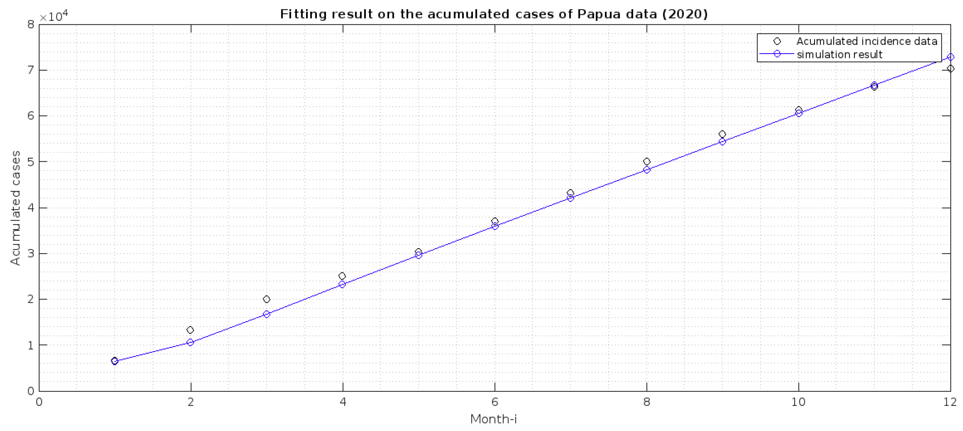
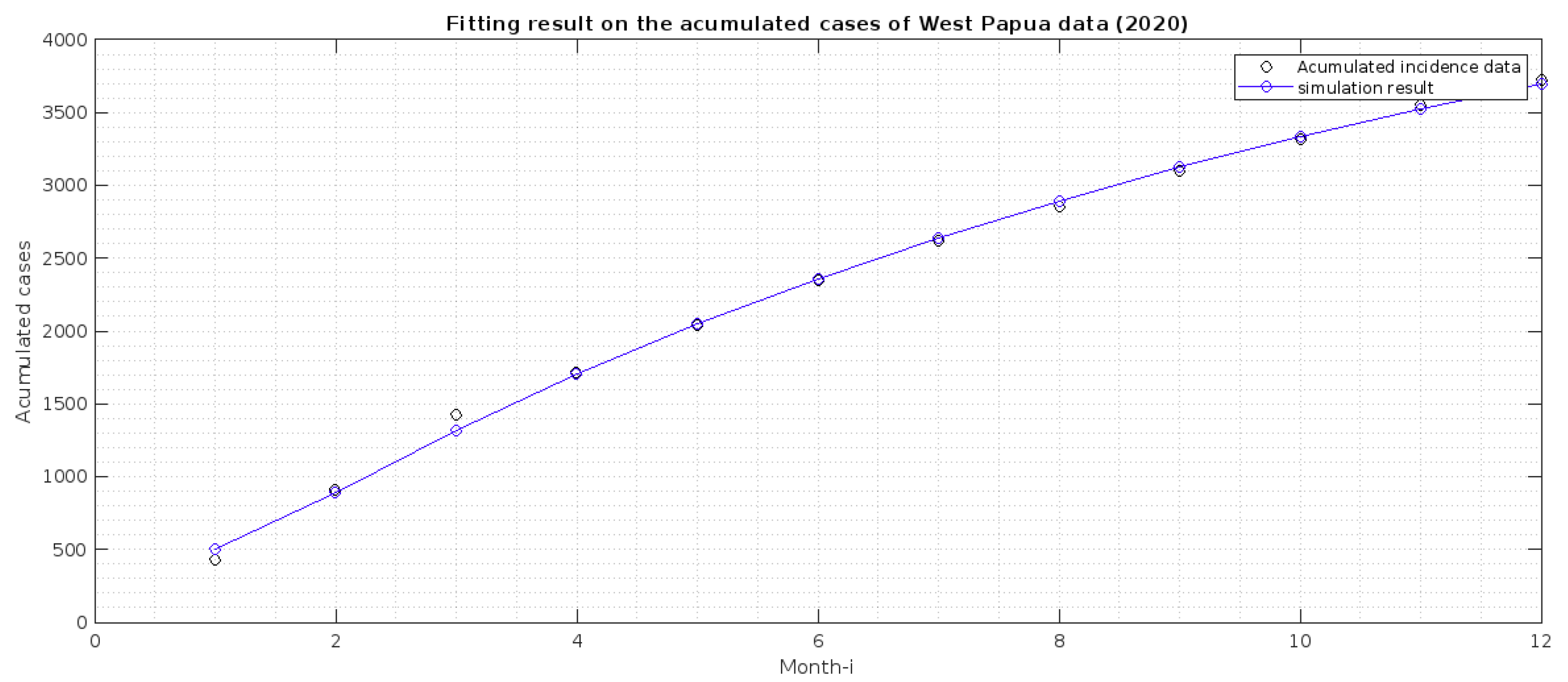
2.2. Parameter Estimation

In this section, we discuss the incidence data that we use to estimate our parameters and the numerical scheme that has been used. The incidence data for malaria are taken from two provinces in Indonesia that have the highest number of malaria incidence every year, namely Papua and West Papua [44]. According to [32,33], the total number of inhabitants in Papua and West Papua was 3,435,430 and 981,822 in 2020, respectively. In both areas, the majority of malaria cases are caused by Plasmodium falciparum, and Plasmodium vivax, both of which cause routine health problems and morbidity in these areas [45].
The incidence data used in this article is the monthly new cases in both provinces, from January to December 2020. The data was collected by personal request from the Directorate of Prevention and Control of Vector and Zoonotic Infectious Diseases, Ministry of Health of the Republic of Indonesia. The data can be seen in Figure 2.
In our model, we do not have a compartment that describes the monthly cases of malaria. Hence, we need to adapt our model to accommodate this. Hence, we transform the monthly cases in both provinces into the accumulated case. Next, we create a new compartment from our model, which describes the accumulated cases. From the transmission diagram given in Figure 1, the total detected cases are coming from the compartment T. Hence, the newly detected cases come from the intervention of transmission-blocking from I to T with a rate of u 2 . Hence, the dynamic of the monthly cases is given by
d c d t = u 2 I .
Solving the above differential equation will give us the accumulated cases of malaria incidence. Our task is to minimize the Euclidean distance between c ( t ) from our numerical results with the incidence data, using the best-fit parameter of our model. This task can be formulated as follows.
min X 0 t f c ( t ) simulation c ( t ) data 2 d t ,
where X is the set of best-fit parameters and initial conditions, while t f is the final time of available data. However, because the use of pre-erythrocytic vaccines had not been implemented in Papua and West Papua in 2020, parameter estimation is performed when the parameters u 1 , α , β h 2 , δ 2 , and ζ e 2 are zero and the S 2 and E 2 compartments are zero. The corresponding best-fit parameters are κ , ϑ , β h 1 ¯ , b , δ 1 , p , q , u 2 , γ 1 , γ 2 , β v ¯ , ζ e 1 , ζ t , ζ r , and all initial conditions of the system (1) (except S 2 ( 0 ) and E 2 ( 0 ) ) and (3). We used a nonlinear optimization toolbox in MATLAB to conduct this parameter estimation, called fmincon function. To run the simulation, we need to give an estimation of an interval in which our parameter values must exist. Hence, we use the lower and upper bound of our parameter values, calculated as shown in Table 2. We estimate our parameter values for incidence data in Papua and West Papua, and the result is given in Table 1, while the fitted cumulated cases are in Figure 2 and Figure 3. This finding indicates that malaria incidence will increase in Papua Province, which tends to the malaria-endemic equilibrium point. Meanwhile, malaria incidence in West Papua Province tends to the malaria-free equilibrium point. From our modeling analyses/results, we can deduce the following:
1.
Papua is more malaria-endemic than West Papua given the non-controlled basic reproduction number ( R 0 | Papua = 1.75 and R 0 | West Papua = 1.53 ). See the formula of non-controlled basic reproduction number ( R 0 ) in (12).
2.
Based on the value of p and q, we conclude that individuals in Papua have a slightly bigger chance of reaching the malaria elimination target if there is a continuous implementation of treatment efforts compared to West Papua.
3.
The infection rates from mosquitoes to humans ( β h 1 , and β h 2 ) in West Papua is higher than in Papua. Hence, it is important to develop a media campaign that targets reducing the contact between humans and mosquitoes in West Papua than in Papua. Such campaigns may include the use of bed nets or mosquito repellent.

3. Dynamical Analysis of the Model

3.1. Preliminary Results on the Positiveness and Boundedness of the Solution

The malaria model in system (1) involves human and mosquito populations. Hence, it is necessary to guarantee that all associated variables are positive with nonnegative parameters and initial conditions.
Theorem 1.
Let the initial conditions of all variables in system (1) be nonnegative as follows:
S 1 ( 0 ) > 0 , S 2 ( 0 ) 0 , E 1 ( 0 ) 0 , E 2 ( 0 ) 0 , I ( 0 ) 0 , T ( 0 ) 0 , R 1 ( 0 ) 0 , T 2 ( 0 ) 0 , V ( 0 ) > 0 , W ( 0 ) 0 .
Then the solution set
Ω = S 1 ( t ) , S 2 ( t ) , E 1 ( t ) , E 2 ( t ) , I ( t ) , T ( t ) , R 1 ( t ) , R 2 ( t ) , V ( t ) , W ( t )
is nonnegative for all t 0 .
Proof. 
Let β h 1 S 1 W + ( u 1 + μ h ) S 1 = G ( t ) . Since the initial conditions of R 1 , R 2 , and S 2 are nonnegative, then the first equation in system (1) satisfies:
d S 1 ( t ) d t = Π h G ( t ) S 1 ( t ) + κ R 1 + ϑ R 2 + α S 2 Π h G ( t ) S 1 ( t ) .
Hence, we have:
d S 1 ( t ) d t + G ( t ) S 1 ( t ) Π h .
Choosing the integrating factor as exp 0 t G ( τ ) d τ . gives us:
d S 1 ( t ) d t exp 0 t G ( τ ) d τ + G ( t ) S 1 ( t ) exp 0 t G ( τ ) d τ Π h exp 0 t G ( τ ) d τ d d t S 1 ( t ) exp 0 t G ( τ ) d τ Π h exp 0 t G ( τ ) d τ .
Integrating both sides yields
S 1 ( t ) exp 0 t G ( τ ) d τ S 1 ( 0 ) Π h 0 t exp 0 τ G ( u ) d u d t .
Therefore,
S 1 ( t ) S 1 ( 0 ) exp 0 τ G ( u ) d u + Π h 0 t exp 0 τ G ( u ) d u d t exp 0 τ G ( u ) d u 0 .
Therefore, we can see that if S 1 ( 0 ) > 0 , then we have that S 1 ( t ) 0 for all t > 0 . A similar approach can be used to show that S 2 ( t ) , E 1 1 ( t ) , E 2 ( t ) , I ( t ) , R 1 ( t ) , R 2 ( t ) , V ( t ) , and W ( t ) are nonnegative for all t 0 . This completes the proof. □
It can be shown that our model in system (1) is well-defined biologically in the feasible region below.
Ω = ( X ( t ) , Y ( t ) ) R + 8 × R + 2 | 0 N ( t ) Π h μ h , 0 V ( t ) + W ( t ) Π v μ v ,
where X ( t ) = { S 1 ( t ) , S 2 ( t ) , E 1 ( t ) , E 2 ( t ) , I ( t ) , T ( t ) , R 1 ( t ) , R 2 ( t ) } and Y ( t ) = { V ( t ) , W ( t ) } .

3.2. The Malaria-Free Equilibrium and the Controlled Reproduction Number

The first equilibrium point of malaria model in (1) is the malaria-free equilibrium, which is denoted by E * , and given by
E * = ( S 1 0 , S 2 0 , E 1 0 , E 2 0 , I 0 , T 0 , R 1 0 , R 2 0 , V 0 , W 0 ) = ( α + μ h ) Π h μ h ( α + μ h + u 1 ) , u 1 Π h μ h ( α + μ h + u 1 ) , 0 , 0 , 0 , 0 , 0 , 0 , Π v μ v , 0 .
It can be seen that E * presents a condition where all infections have disappeared from both populations. In this condition, we also can see that the ratio of susceptible human beings with and without pre-erythrocytic vaccine is given by
S 1 0 S 2 0 = ( α + μ h ) Π h μ h ( α + μ h + u 1 ) u 1 Π h μ h ( α + μ h + u 1 ) = ( α + μ h ) Π h u 1 Π h = α + μ h u 1 .
The purpose is, of course, to reduce this ratio, which is equivalent to increasing the number of individuals in S 2 . It can be seen that this ratio is only affected by three parameters, namely μ h , α , and u 1 . Of these three parameters, only the latter two are controllable. Therefore, we can see that reducing this ratio can be done by increasing the rate of vaccination, and the vaccine’s duration could be prolonged. Hence, the higher the quality of the vaccine (i.e., its duration), the better.
We will now calculate the basic and controlled reproduction number of our model, which is denoted by R 0 and R C , respectively. The basic reproduction number defines the expected average number of secondary malaria cases caused by a single malaria-infected case during its infection period in a completely susceptible population. This threshold holds a vital role in many malaria models [48]. From its definition, R 0 helps us to understand the qualitative behavior of our model and whether the disease may persist or exist. Mostly, they found that malaria will disappear from the population if R 0 < 1 , and exist if R 0 > 1 . In several cases, mainly when backward bifurcation phenomena occur in their model [18,49,50,51], it is still possible to find malaria even though R C is already less than one.
When no control intervention is given to our model, then system (1) reduced into:
d S 1 d t = Π h + κ R 1 β h 1 S 1 W μ h S 1 ,
d E 1 d t = β h 1 S 1 W ( δ 1 + μ h ) E 1 ,
d I d t = δ 1 E 1 ( γ 1 + μ h ) I ,
d R 1 d t = γ 1 I ( κ + μ h ) R 1 ,
d V d t = Π v β v ( ζ e 1 E 1 + I + ζ r R 1 ) V μ v V ,
d W d t = β v ( ζ e 1 E 1 + I + ζ r R 1 ) V μ v W .
To find the basic reproduction number of the basic model (Section 3.2), we use the well known next-generation matrix approach [52]. The respected basic reproduction number for the basic model (11) is given as follows.
R 0 = Π h β h 1 μ h μ v × β v ζ e 1 π v μ v δ 1 + μ h + β v π v δ 1 μ v δ 1 + μ h γ 1 + μ h + β v ζ r Π v δ 1 γ 1 μ v δ 1 + μ h γ 1 + μ h κ + μ h .
With a similar approach, we can calculate the controlled reproduction number of our malaria problem. Implementing the next-generation matrix method into system (1), the controlled reproduction number is given by:
R C = f a + g b + h c + i d + j e ,
where
f a = Π v μ v · β v ζ e 1 μ v R 0 v E 1 · Π h μ h · α + μ h α + μ h + u 1 · β h 1 δ 1 + μ h R 0 h 1 E 1 ,
g b = Π v μ v · β v ζ e 2 μ v R 0 v E 2 · Π h μ h · u 1 α + μ h + u 1 · β h 2 δ 2 + μ h R 0 h 2 E 2 ,
h c = Π v μ v · β v μ v R 0 v I · Π h μ h K R 0 h I ,
i d = Π v μ v · β v ζ t μ v R 0 v T · Π h μ h α + μ h α + μ h + u 1 · β h 1 δ 1 + μ h · δ 1 u 2 L + u 1 α + μ h + u 1 · β h 2 δ 2 + μ h · δ 2 u 2 L R 0 h T ,
j e = Π v μ v · β v ζ r μ v R 0 v R 1 · Π h μ h M R 0 h R 1 ,
and
K = α + μ h α + μ h + u 1 · β h 1 δ 1 + μ h · δ 1 γ 2 + μ h L + u 1 α + μ h + u 1 · β h 2 δ 2 + μ h · δ 2 γ 2 + μ h L , M = α + μ h α + μ h + u 1 · β h 1 δ 1 + μ h · δ 1 κ + μ h · u 2 γ 2 q + γ 2 γ 1 + μ h γ 1 L + u 1 α + μ h + u 1 · β h 2 δ 2 + μ h · δ 2 κ + μ h · u 2 γ 2 q + γ 2 γ 1 + μ h γ 1 L , L = p γ 2 u 2 + q γ 2 u 2 + γ 1 γ 2 + γ 1 μ h + γ 2 μ h + μ h 2 + μ h u 2 .
As we can see from the expression on (13), R 0 is the combination of many paths of infection on our model. The explanation is given as follows.
1.
R 0 v E 1 shows the path of transmission for a new case in mosquito due to a bite from susceptible mosquitoes to an exposed human in compartment E 1 .
2.
R 0 h 1 E 1 shows the transmission path which gives a new infection in humans without pre-erythrocytic vaccine ( E 1 ) due to a bite from infected mosquitoes.
3.
R 0 v E 2 presents the transmission path for a new infection in the mosquito population after they bite exposed humans in E 2 .
4.
R 0 h 2 E 2 presents the transmission path for a new infection in vaccinated human E 2 due to a bite from infected mosquitoes.
5.
R 0 v I shows a transmission for a new infection in the mosquitoes population after biting an infected individual in I.
6.
R 0 h I presents a transmission path for a new cases in I due to progression of E 1 and E 2 .
7.
R 0 v T presents a transmission path for a new case in the mosquitoes population after biting an infected individual who is undergoing treatment ( T ) .
8.
R 0 h T presents a transmission path for a new case in treated human population ( T ) due to the treatment rate from I.
9.
R 0 v R 1 presents a transmission path for a new case in the mosquito population after biting individuals in R 1 .
10.
R 0 h R 1 presents a transmission path for new cases in the compartment of humans who partially succeed in conducting transmission-blocking treatment.

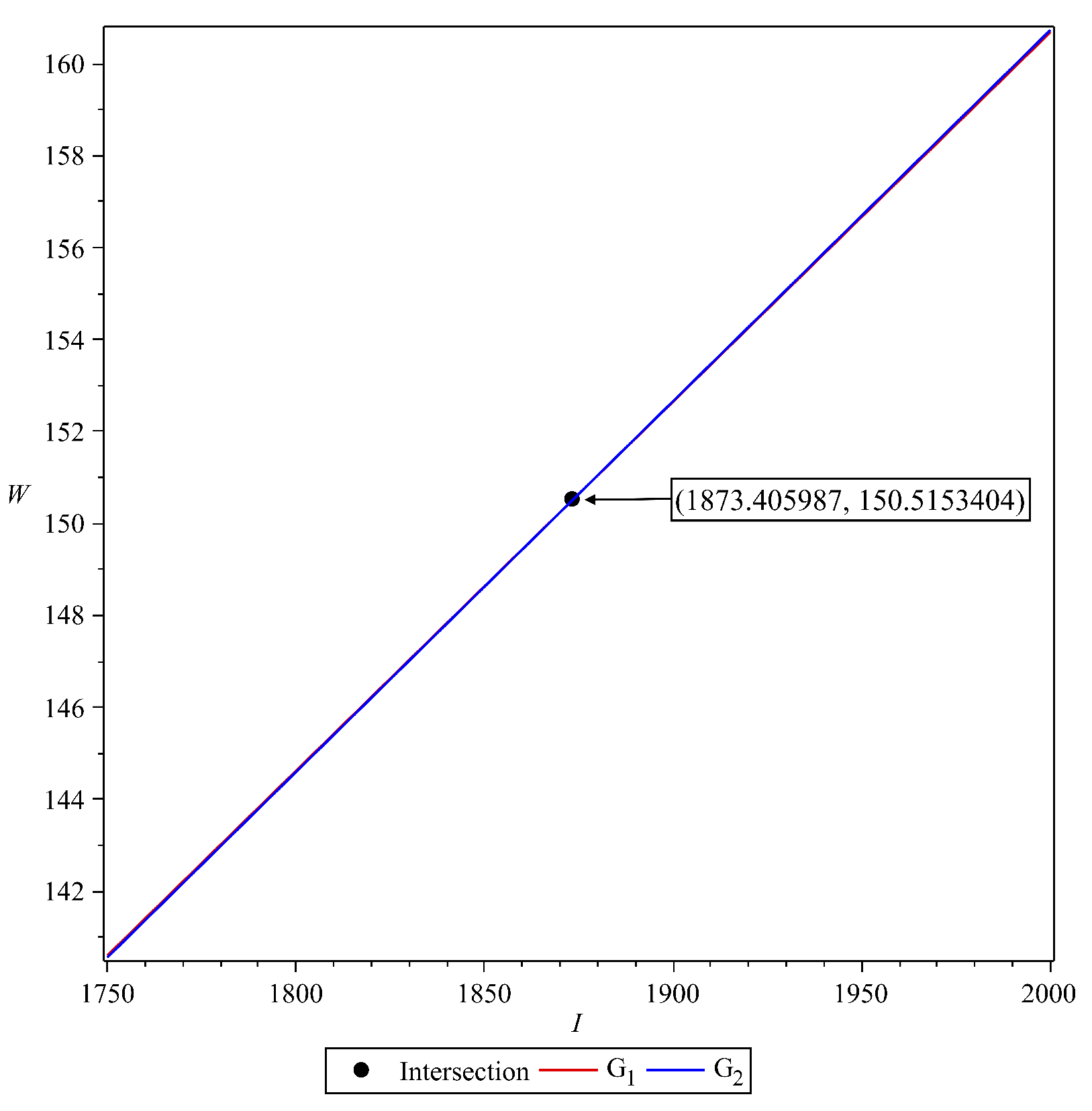
3.3. The Malaria-Endemic Equilibrium

The malaria-endemic equilibrium point of system (1) indicates the condition when malaria persists in the human and mosquito populations. The malaria-endemic equilibrium of system (1) will be determined when the number of infected individuals is not equal to zero. However, due to the complexity of the model, we can not explicitly show the form of the endemic equilibrium point as a function of other parameters. Hence, we write our endemic equilibrium point as a function of dependent variables I and W. The idea is as follows. We set the right hand side of system (1) equal to zero, and solve them backwardly with respect to each variables until we only have I and W left. This process will give us two different polynomial as a function of I and W. Hence, the malaria-endemic equilibrium of system (1) is given by:
E = ( S 1 * , S 2 * , E 1 * , E 2 * , I * , T * , R 1 * , R 2 * , V * , W * ) ,
where
S 1 * = W * β h 2 + α + μ h I * δ 2 + μ h δ 1 + μ h a W * ,
S 2 * = u 1 I * δ 2 + μ h δ 1 + μ h a W * ,
E 1 * = W * β h 2 + α + μ h I * δ 2 + μ h β h 1 a ,
E 2 * = u 1 I * β h 2 δ 1 + μ h a ,
T * = u 2 I * γ 2 + μ h ,
R 1 * = q u 2 + γ 1 γ 2 + γ 1 μ h I * γ 2 + μ h κ + μ h ,
R 2 * = I * p γ 2 u 2 γ 2 + μ h μ h + ϑ ,
V * = μ v W * β v T * ζ t + E 1 * ζ e 1 + E 2 * ζ e 2 + R 1 * ζ r + I * ,
with
a = μ h 2 + γ 1 + γ 2 + u 2 μ h + γ 2 p + q u 2 + γ 1 γ 2 + μ h × 1 β h 1 δ 1 μ h 2 + δ 1 W * β h 2 + α + δ 2 β h 1 + u 1 δ 2 β h 2 μ h + δ 2 W * β h 2 + α β h 1 + β h 2 u 1 δ 1 ,
while I * and W * are taken from the positive intersection of the following polynomials:
G 1 = a 2 ( I ) W 2 + a 1 ( I ) W + a 0 ( I ) = 0 , G 2 = b 1 ( W ) I + b 0 ( W ) = 0 ,
where a i ( I ) , b i ( W ) for i = 0 , 1 , 2 has a complex form to be shown. We leave the existence analysis on this malaria-endemic equilibrium as an open problem to an interested reader.
We show the existence of this malaria-endemic equilibrium numerically with the following scenario. To conduct this numerical experiment, we use the following parameter values:
Using the above parameter values, we have the basic reproduction number of system (1) is 1.002169498 , which is larger than one. Substituting the parameter values in Table 3 into G 1 and G 2 yield:
G 1 = ( 2.81 × 10 19 I + 2.4 × 10 11 ) W 2 + ( 1.89 × 10 12 I + 3.62 × 10 6 ) W 2.91 × 10 7 I = 0 , G 2 = 6.14 × 10 15 ( W + 150489.34 ) ( W + 34834.79 ) I 2.67 × 10 9 ( W + 150616.39 ) W = 0 .
Next, we plot G 1 and G 2 in I W plane. The result is given in Figure 4.
Since we have an intersection between G 1 and G 2 in the first quadrant of I W plane, then we have the malaria-endemic equilibrium point, which is given by:
E = ( S 1 * , S 2 * , E 1 * , E 2 * , I * , T * , R 1 * , R 2 * , V * , W * ) = 3400396 , 20241 , 200 , 2 , 1874 , 862 , 1960 , 9898 , 6870710 , 151 .

4. Sensitivity Analysis

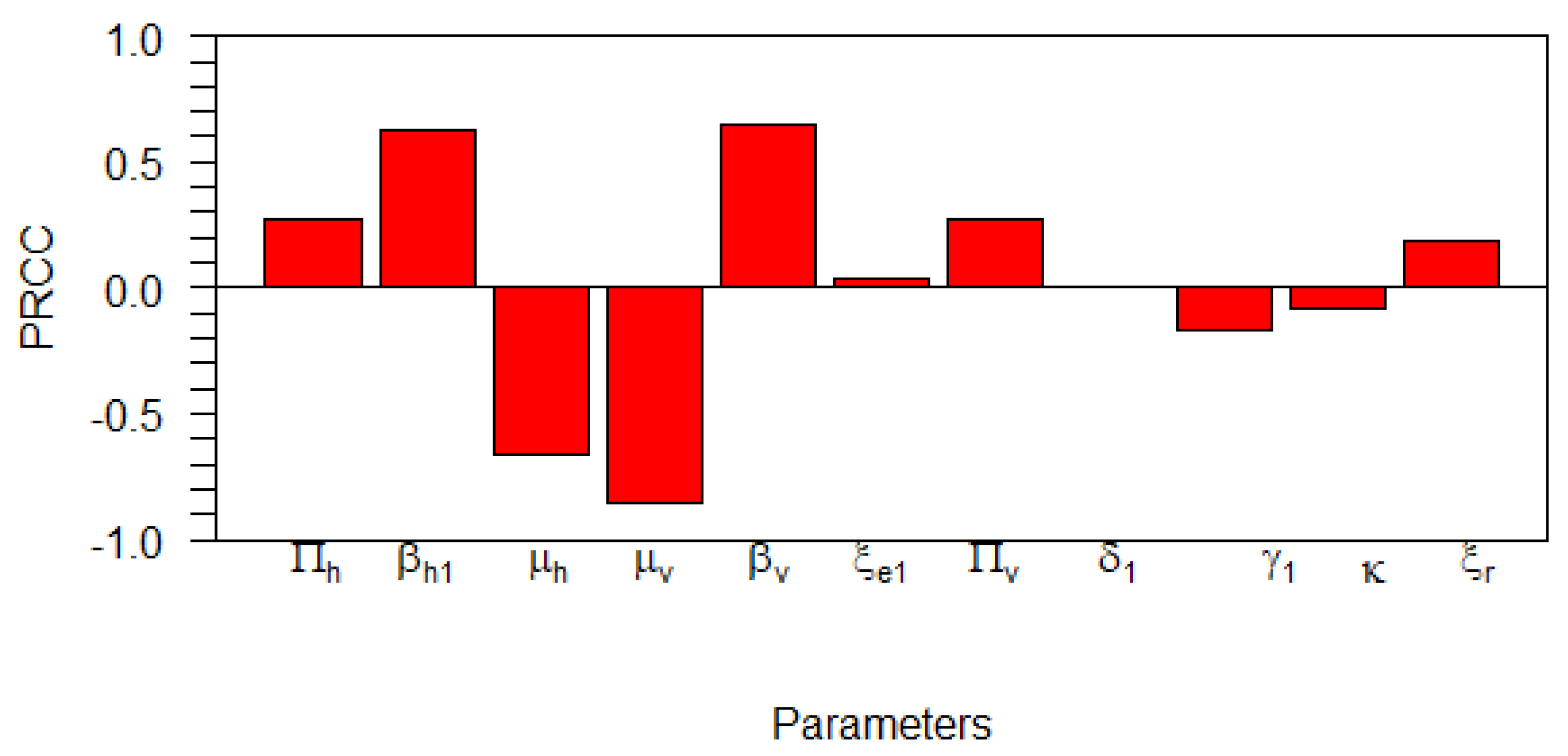
4.1. Global Sensitivity Analysis on the Basic Reproduction Number

In this subsection, we carry out a global uncertainty analysis of basic reproduction number for the malaria model without control. As we have already shown in the previous section, the basic reproduction number could determine whether malaria will persist or become extinct in the population. Hence, it is essential to analyze the sensitivity of the basic reproduction number with respect to the model parameters. Global sensitivity analysis is used to study the relative changes in epidemic model parameters output, giving input/altered model parameters for the dynamical systems under investigation. Thus, we enabled modelers to identify key model variables that require controlling for the particular disease. To carry out the simulation, we used global sensitivity analysis, which combines the Latin-hypercube sampling and Partial Rank Cross Correlation (PRCC) technique as given in [53] with similar analysis in [54]. Using R-software, we performed 1000 simulations per run, and examined and evaluated the PRCC of the model parameters concerning in R 0 . The PRCC indicates the degree of monotonicity between the model’s parameters in the R 0 . Thus, juxtaposing the values of PRCC gives an apparent effect and contribution of each model parameter on R 0 in our malaria model. The results from the numerical simulations are given in Figure 5 and Table 4. The sensitivity of the parameters to the basic reproduction number (12) is proportional to the absolute value of PRCC. As we can see in Table 4, we observe Π h , β h 1 , μ h , μ v , β v , Π v , γ 1 , and ξ r . From these parameters, we can see that β h 1 , β v , and μ v are the most significant parameters that can be controlled. Increasing μ v and reducing β h 1 and β v will reduce R 0 . It can also been seen in Table 4 that all the parameters have p-values < 0.05 and thus are said to be significant besides ξ e 1 , κ , and δ 1 . Therefore, it is essential to introduce intervention to reduce the infection rate with vaccine in susceptible populations, or increasing the mosquito death rate with fumigation.

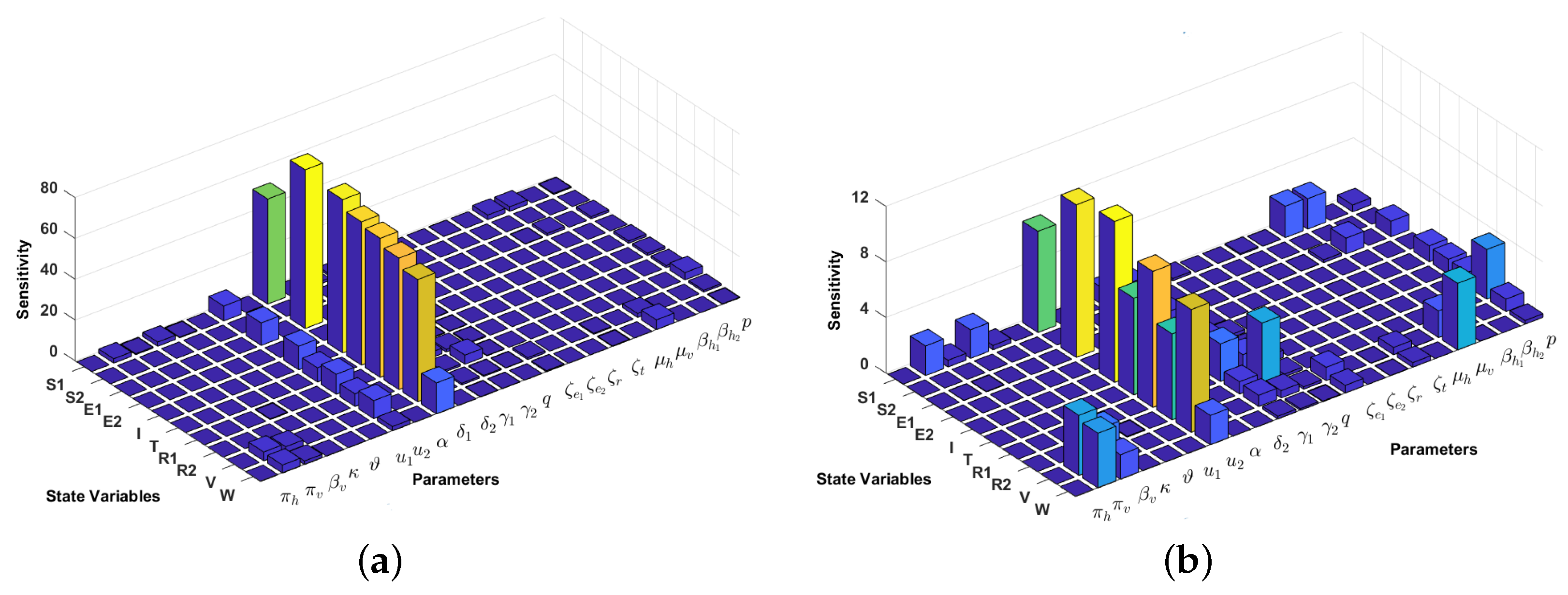
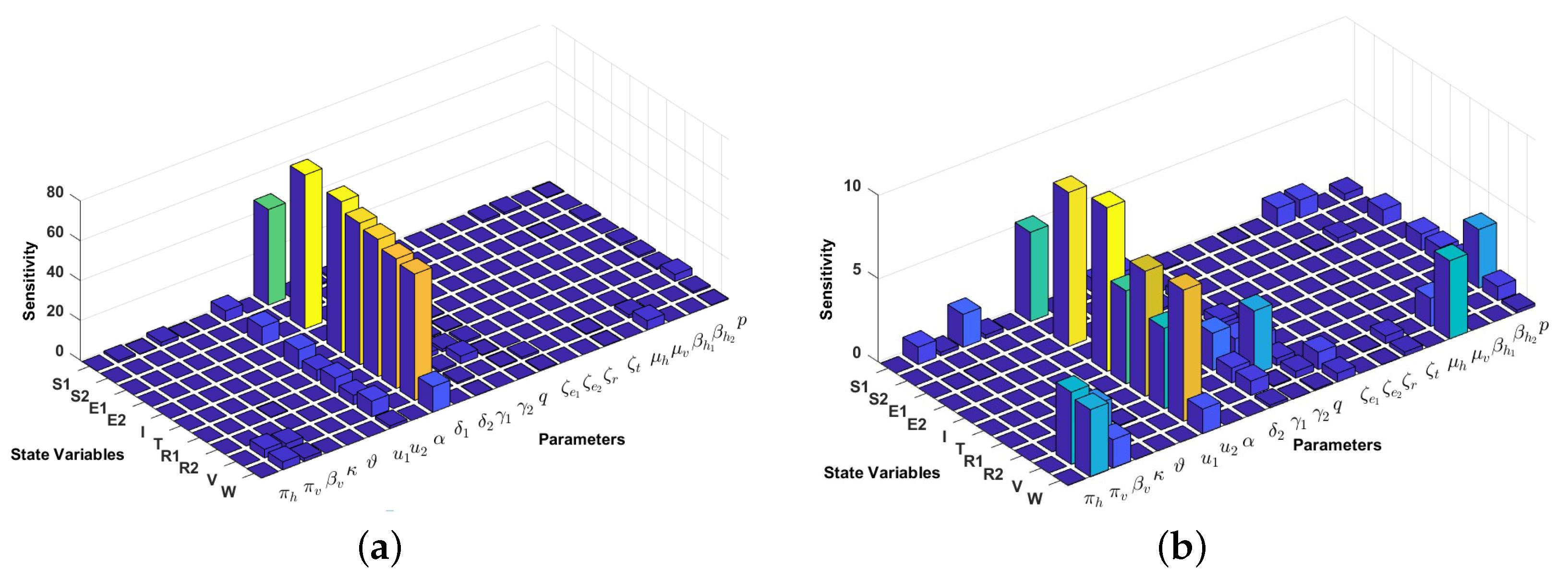
4.2. Local Sensitivity Analysis on the Model Variables

The sensitivity methods can be used on infectious disease models to determine which variable or parameter is sensitive to a specific condition. In our case, identifying the key critical parameters of system (1) is an effective way to study the qualitative behaviour of the parameters which govern the model. In our proposed model (1), we have 10 compartments x i for i = 1 , 2 , . . . , 10 and 22 parameters k j for j = 1 , 2 , . . . , 22 . Then, the local sensitivities can be calculated using three different techniques: non-normalisations, half-normalizations, and full-normalizations. Firstly, the equation of non-normalization sensitivities is given by
S k j x i = x i k j ,
where S k j x i is measured as sensitivity coefficients of each x i with respect to each parameter k j . Then, the formula of half–normalization sensitivities is defined below:
S k j x i = 1 x i x i k j .
Finally, the equation of full-normalization sensitivities is defined by
S k j x i = k j x i x i k j .
In this article, we only perform a full-normalization sensitivity analysis on our proposed model in (1) for best-fit parameter of Papua and West-Papua incidence data. The results are given in Figure 6 and Figure 7. We can see from Figure 6 and Figure 7 that the progression rate from E 1 to I ( δ 1 ) is the most influential parameter for all compartments, except S 2 and E 2 . The second most influential parameter is the transmission-blocking parameter ( u 2 ) . In contrast to u 2 , we can see that the impact of pre-erythrocytic ( u 1 ) is not as sensitive as u 2 . This result is similar to our previous sensitivity analysis on R 0 .

5. Existence of Solution and Characterization of the Optimal Control Problem

We consider our optimal control problem on determining S 1 * , S 2 * , E 1 * , E 2 * , I * , T * , R 1 * , R 2 * , V * , W * , associated with our admissible control parameter ( u 1 * , u 2 * ) Ω on the time interval [ 0 , T ] , which satisfies our malaria model in (1), non-negative initial conditions S 1 ( 0 ) , S 2 ( 0 ) , E 1 ( 0 ) , E 2 ( 0 ) , I ( 0 ) , T ( 0 ) , R 1 ( 0 ) , R 2 ( 0 ) , V ( 0 ) , and W ( 0 ) in order to minimize the cost function in (2), i.e.,
J ( u 1 * , u 2 * ) = min Ω J ( u 1 , u 2 ) .
The existence of our optimal control solutions ( u 1 * , u 2 * ) comes from the convexity of the integrand of the cost function in (2) with respect to the controls and the regularity of the malaria model in (1) (See [55,56] for the existence results of optimal solutions).

5.1. Existence of the Optimal Solution

In this subsection we state and prove the existence of solutions for the optimal control ODE system given in Equation (1), before proving the existence of solutions for the optimal control problem. Firstly, it is necessary to establish the boundedness of our malaria model over the modeling time horizon. Now, let S ^ 1 , S ^ 2 , E ^ 1 , E ^ 2 , I ^ , T ^ , R ^ 1 , R ^ 2 , V ^ , and W ^ denote the super-solutions with respect to each state variable in Equation (1). Therefore, we obtain
d S ^ 1 d t = Π h ,
d S ^ 2 d t = S ^ 1 ,
d E ^ 1 d t = 1 ,
d E ^ 2 d t = 1 ,
d I ^ d t = δ 1 E ^ 1 + δ 2 E ^ 2 ,
d T ^ d t = I ^ ,
d R ^ 1 d t = γ 1 I ^ + q γ 2 T ^ ,
d R ^ 2 d t = p γ 2 T ^ ,
d V ^ d t = 1 ,
d W ^ d t = β v ( ζ e 1 E ^ 1 + ζ e 2 E ^ 2 + I ^ + ζ t T ^ + ζ r R ^ 1 ) .
Writing system (24) in a vector notation format, we get
X ¯ = M 1 X ¯ + M 2 ,
where X ¯ = S ^ 1 S ^ 2 E ^ 1 E ^ 2 I ^ T ^ R ^ 1 R ^ 2 V ^ W ^ , M 1 0 0 0 0 0 0 0 0 0 0 1 0 0 0 0 0 0 0 0 0 0 0 0 0 0 0 0 0 0 0 0 0 0 0 0 0 0 0 0 0 0 0 0 0 δ 1 δ 2 0 0 0 0 0 0 0 0 0 1 0 0 0 0 0 0 0 0 q γ 2 γ 1 0 0 0 0 0 0 0 0 p γ 2 γ 1 0 0 0 0 0 0 0 0 0 0 0 0 0 0 0 0 β v ζ e 1 β v ζ e 2 1 β v ζ t β v ζ r 0 0 0 and
M 2 = Π h 0 1 1 0 0 0 0 1 0 .
From the above matrices, it can be deduced that our model is linear and satisfies the properties of being semi-positive definite on Ω . Then, it follows that the super-solutions of the system (1) are bounded.
Applying Theorem 4.1 on pages 68–69 of Fleming and Rishel [56], we then show the existence of the optimal control model. Supposed
H = { u k ( t ) : 0 u k ( t ) 1 } , t [ 0 , t f ] f o r k = 1 , 2 .
Theorem 2.
Given the objective functional
J = 0 t f ω 1 u 1 2 + ω 2 u 2 2 + ω 3 I + ω 4 R 1 d t ,
which has associated admissible control while subject to the model initial conditions given in Theorem 1. There exists an optimal control pair u 1 * , u 2 * which minimizes the functional
J ( u 1 * , u 2 * ) = min Ω J ( u 1 , u 2 ) .
Therefore, the conditions enumerated below should be satisfied by our model.
1. 
The admissible control parameters and each model state variable are non-empty.
2. 
Control H is convex and bounded.
3. 
Right hand side of our system is continuous and bounded above by a linear function in the state variables and the control parameters.
4. 
The integrand of J ( u 1 ( t ) , u 2 ( t ) ) is concave on H .
5. 
There exists positive constants b 1 , b 2 > 0 and τ > 1 such that J ( u k ( t ) ) satisfies
J ( u 1 ( t ) , u 2 ( t ) ) b 1 + b 2 ( | u 1 | 2 + | u 2 | 2 ) τ 2 .
Proof. 
The proof follows for the stated conditions as follows:
1.
Applying the methodology of Theorem 9.2.1 on page 182 of [57], the first criteria is fulfilled as the solutions of our model system exist and are bounded in ω as also shown by the existence of the super-solutions.
2.
Using the definition of H , we have that set as bounded and closed.
3.
Considering our model in Equation (1) and the cost function (2) is linear in u 1 and u 2 . with the aid of the result of the theorem as in [57], we can then deduce that the right-hand side of our system is continuous and bounded.
4.
Suppose the objective function
L = ω 1 u 1 2 + ω 2 u 2 2 + ω 3 I + ω 4 R 1
and we set ( p , q ) Θ , for p , q and 0 t 1 . Then L ( t p + ( 1 t ) p ) t ( p ) + ( 1 t ) L p . Additionally, let ( p , q ) Θ 2 for 0 t 1 , then we have that p = u 11 ,   p = u 12 and ( t p + ( 1 t ) q = t u 11 + ( 1 t ) u 12 ) . Thus,
L ( t p + ( 1 t ) q ) = ω 3 I + ω 4 R 1 + ω 1 ( t u 11 + ( 1 t ) u 12 ) 2 + ω 2 ( t u 21 + ( 1 t ) u 22 ) 2
t L ( p ) + ( 1 t ) L ( q ) = ω 3 I + ω 4 R 1 + ω 1 ( t u 11 2 + ( 1 t ) u 12 2 ) + ω 2 ( t u 21 2 + ( 1 t ) u 22 2 ) .
From (2), we observe that
( t u 11 + ( 1 t ) u 12 ) 2 ( t u 11 2 + ( 1 t ) u 12 2 ) ,
( t u 21 + ( 1 t ) u 22 ) 2 ( t u 21 2 + ( 1 t ) u 22 2 ) .
Following this observation, we can then generalize that given any ( p , q ) θ 2 for 0 t 1 we obtain L ( t p + ( 1 t ) q ) t L ( p ) + ( 1 t ) L ( q ) . Hence, the integrand of J is concave.
5.
Following the fact that the model state variable in the objective function, that is, I and R 1 are bounded as shown in 3. Above, there exits positive constants φ 1 , φ 2 > 0 such that the sum of ( I + R 1 ) φ 2 . If we set φ 2 = max n = 3 , 4 , we have that
L ( I , R 1 , u 1 , u 2 ) η 1 + η 2 + η 3 | u 1 2 | + | u 2 2 | 2 τ
in which τ = 2 . This implies that there is a positive constant φ 1 , φ 2 > 0 and a τ > 1 such that the integrand component of J satisfies
L ( I , R 1 , u 1 , u 2 ) φ 1 + φ 2 | u 1 2 | + | u 2 2 | 2 σ .
From the above proof, we have that our system satisfies the necessary conditions in Theorem 2, which is completed here. □

5.2. Characterization of the Optimal Control Problem

The Pontryagin’s Maximum principle [58] allows us to utilize costate functions to transform the optimization problem to the problem of determining the point-wise minimum of u 1 * and u 2 * of the Hamiltonian. This Hamiltonian function is built using the cost function in (2) and the malaria model in (1). With this, we derive:
H ( X , λ j , u i ) = ω 1 u 1 2 + ω 2 u 2 2 + ω 3 I + ω 4 R 1 + λ 1 Π h + κ R 1 + ϑ R 2 + α S 2 β h 1 S 1 W ( u 1 ( t ) + μ h ) S 1 + λ 2 u 1 ( t ) S 1 β h 2 S 2 W ( α + μ h ) S 2 + λ 3 β h 1 S 1 W ( δ 1 + μ h ) E 1 + λ 4 β h 2 S 2 W ( δ 2 + μ h ) E 2 + λ 5 δ 1 E 1 + δ 2 E 2 + ( 1 p q ) γ 2 T ( u 2 ( t ) + γ 1 + μ h ) I + λ 6 u 2 ( t ) I p γ 2 T q γ 2 T ( 1 p q ) γ 2 T μ h T + λ 7 γ 1 I + q γ 2 T ( κ + μ h ) R 1 + λ 8 p γ 2 T ( ϑ + μ h ) R 2 + λ 9 Π v β v ( ζ e 1 E 1 + ζ e 2 E 2 + I + ζ t T + ζ r R 1 ) V μ v V + λ 10 β v ( ζ e 1 E 1 + ζ e 2 E 2 + I + ζ t T + ζ r R 1 ) V μ v W ,
where X = ( S 1 , S 2 , E 1 , E 2 , I , T , R 1 , R 2 , V , W ) and λ j for i = 1 , 2 , 10 are the associated adjoints for the model variables S 1 , S 2 , E 1 , E 2 , I , T , R 1 , R 2 , V , and W, respectively.
Next, we will calculate the optimality system of our optimal control problem. The following results is a direct consequences of application of the Pontriagin’s Maximum Principle for bounded controls [59]. The adjoint system can be written as follows:
d λ 1 d t = L S 1 = β h 1 W ( λ 1 λ 3 ) + u 1 ( λ 1 λ 2 ) + μ h λ 1 , d λ 2 d t = L S 2 = β h 2 W ( λ 2 λ 4 ) + α ( λ 2 λ 1 ) + μ h λ 2 , d λ 3 d t = L E 1 = δ 1 ( λ 3 λ 5 ) + ζ e 1 β v V ( λ 9 λ 10 ) + μ h λ 3 , d λ 4 d t = L E 2 = δ 2 ( λ 4 λ 5 ) + ζ e 2 β v V ( λ 9 λ 10 ) + μ h λ 4 , d λ 5 d t = L I = ω 3 + u 2 ( λ 5 λ 6 ) + γ 1 ( λ 5 λ 7 ) + β v V ( λ 9 λ 10 ) + μ h λ 5 , d λ 6 d t = L T = γ 2 ( λ 6 λ 5 ) + p γ 2 ( λ 5 λ 8 ) + q γ 2 ( λ 5 λ 7 ) + ζ t β v V ( λ 9 λ 10 ) + μ h λ 6 , d λ 7 d t = L R 1 = ω 4 + κ ( λ 7 λ 1 ) + ζ r β v V ( λ 9 λ 10 ) + μ h λ 7 , d λ 8 d t = L R 2 = ϑ ( λ 8 λ 1 ) + μ h λ 8 , d λ 9 d t = L V = β v ( ζ e 1 E 1 + ζ e 2 E 2 + I + ζ t T + ζ r R 1 ) λ 9 λ 10 + μ v λ 9 , d λ 10 d t = L W = β h 1 S 1 ( λ 1 λ 3 ) + β h 2 S 2 ( λ 2 λ 4 ) + μ v λ 10 ,
and with transversality conditions λ j ( T ) = 0 for j = 1 , 2 , 10 . The optimality conditions requires that H u 1 = H u 2 = 0 . Hence, according to our model and cost function, and following the lower and upper bounds, we have:
u 1 * = min max 0 , S 1 ( λ 2 λ 1 ) 2 ω 1 , 1 ,
u 2 * = min max 0 , I ( λ 6 λ 5 ) 2 ω 2 , 1 .

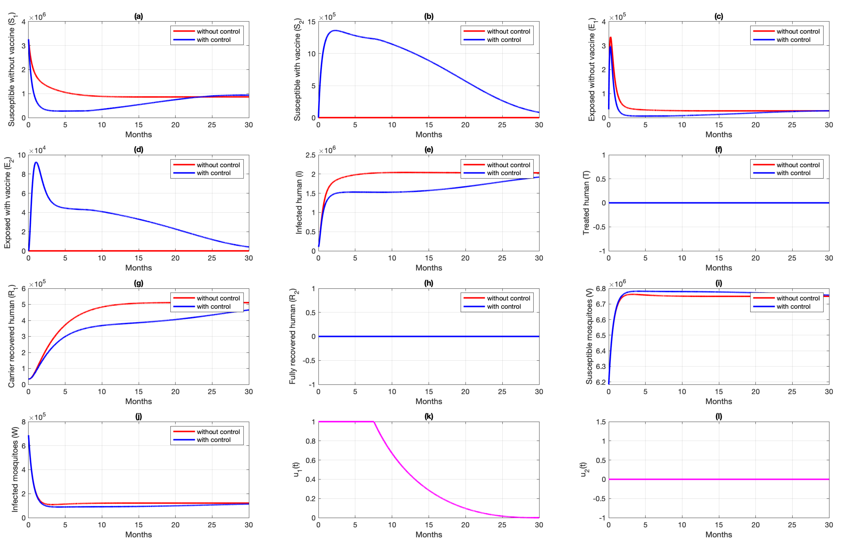
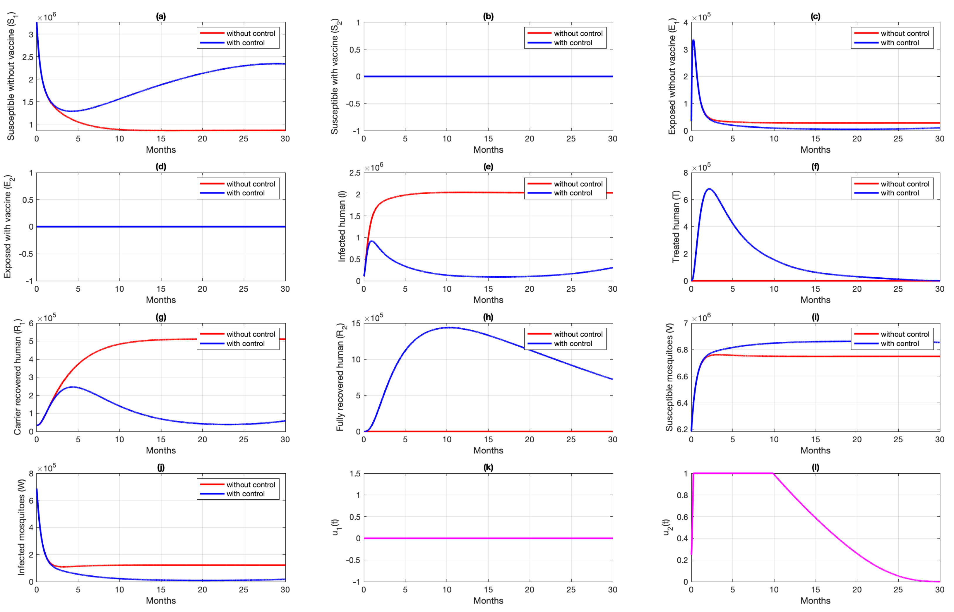
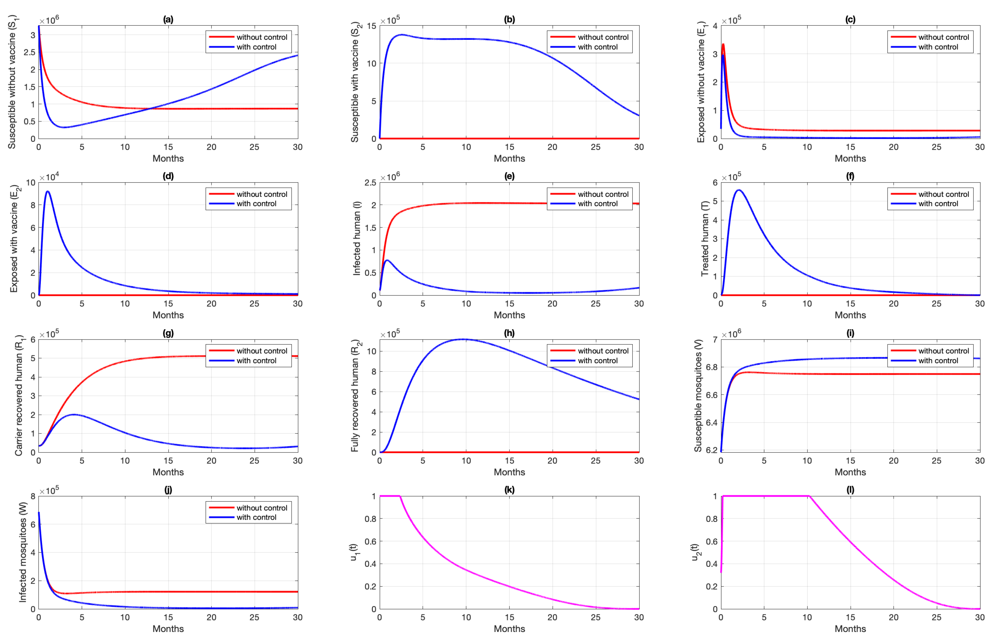
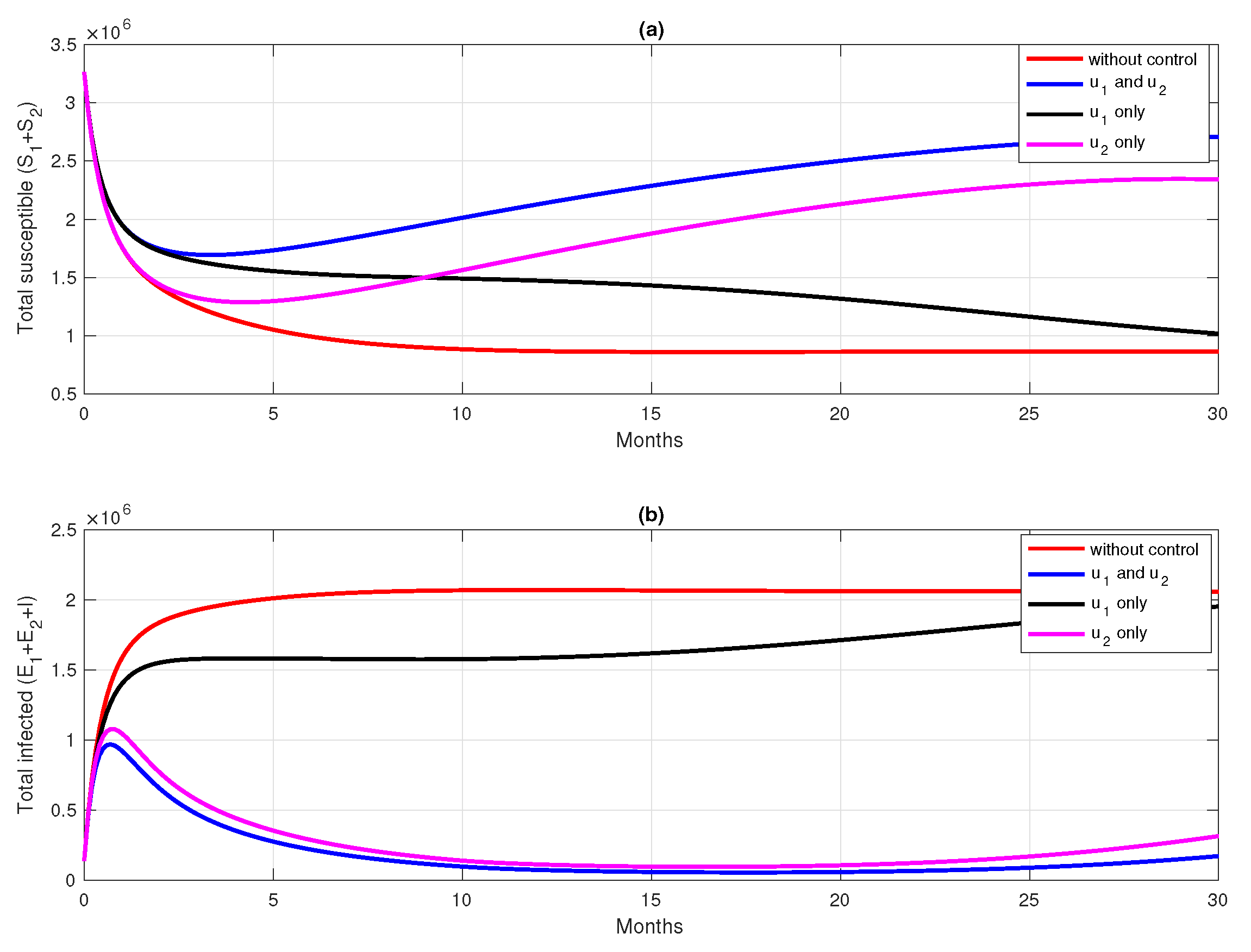
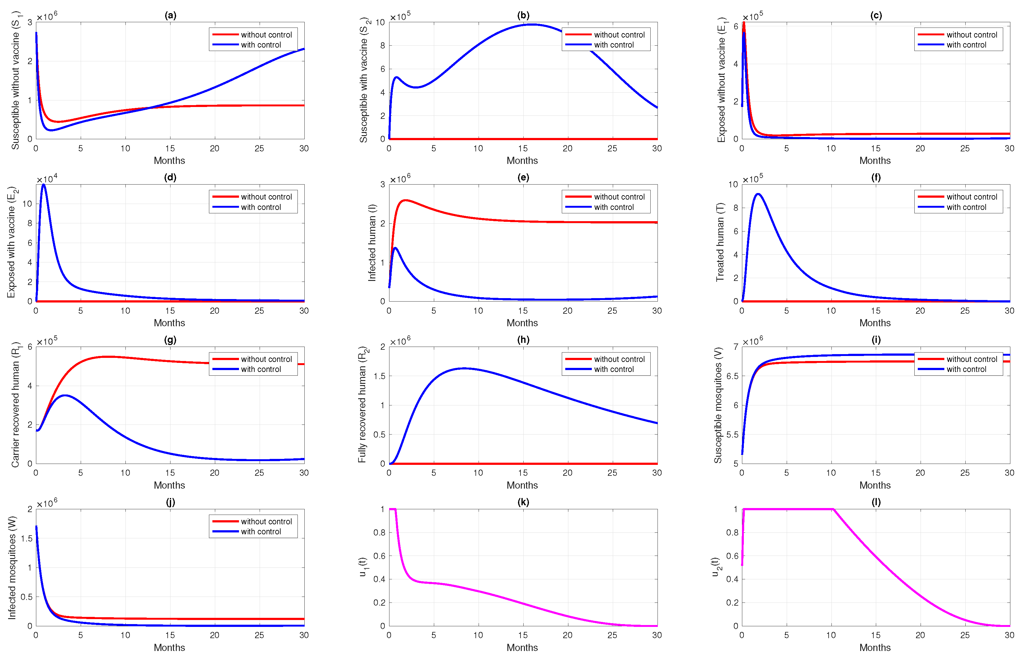
6. Numerical Simulation of the Optimal Control Problem

From the previous analysis, our optimal control problem consists of the state system, which is the malaria model in (1) with initial condition X ( 0 ) , the costate system in (29) with transversality condition λ j ( T ) = 0 , and optimal conditions in (30). To determine the optimal trajectory of u 1 * and u 2 * , we have to determine the solution of the state and costate system. Since the state system has an initial condition, while the costate has the final condition, we cannot solve these systems directly forward in time. Thus, we will solve it using the “forward-backward sweep method” [59]. The algorithm is as follows. An initial guess for the control variables should be made. Then, with this initial guess, we solve the state system in (1) numerically forward in time using a Runge–Kutta method. Having the initial guess of control variables and the solution of the state system for t [ 0 , T ] , we solve our costate system in (29) backward in time, also with the Runge–Kutta method. Having the solution of state and costate for t [ 0 , T ] , we update the control trajectories using the equation in (30). This process is repeated until the convergence criteria are satisfied. In our numerical implementation, the convergence criteria are when the Euclidean distance between i t h and ( i + 1 ) t h iteration for costate, state, and control parameters are smaller than our chosen tolerance.
Unless stated otherwise, to run the simulations in this section, we used parameter values as shown in Table 1, with the following initial conditions: S 1 ( 0 ) = 95 % N , S 2 ( 0 ) = 0 , E 1 ( 0 ) = 1 % N , E 2 ( 0 ) = 0 , I ( 0 ) = 3 % N , T = 0 , R 1 ( 0 ) = 0 , R 2 ( 0 ) = 1 % N , V ( 0 ) = 180 % N , and W ( 0 ) = 20 % N , with N is the total of human population in Papua ( 3,435,430 ) . The values assigned for the weight constant are ω 1 = 1 , ω 2 = 1 , ω 3 = 5 × 10 11 , and ω 4 = 10 12 . In this section, the impact of control trajectories with various scenarios is studied. We studied the impact on the change of the dynamic of each sub-population (with and without controls), the total of susceptible and infected populations, and the cost related to the scenario.

6.1. Different Combination of Interventions

For the first scenario of optimal control simulations, we conducted our experiment based on the combination of controls that have been used. Let Scenarios 1, 2, and 3 be scenarios when only pre-erythrocytic drugs are used ( u 1 > 0 , u 2 = 0 ) , transmission-blocking drugs are used ( u 1 = 0 , u 2 > 0 ) , and both drugs are used ( u 1 > 0 , u 2 > 0 ) , respectively. The illustration on the dynamics of system (1) and the control profiles for Scenarios 1, 2, and 3 are given in Figure 8, Figure 9, and Figure 10, respectively. From Figure 8, we can see that with a profile of u 1 of Scenario 1 in Figure 8k, the number of infected individuals is always decreasing except E 2 , as a consequence of the existence of individuals who are already vaccinated ( S 2 ) . It is clearly observed that the pre-erythrocytic vaccine should be maintained at one from the start of the simulation for a long time period to increase the number of vaccinated individuals. With a large number of vaccinated individuals, fewer people will be infected by mosquitoes. Hence, the total number of infected individuals is always smaller than when no intervention is used. The total cost for Scenario 1 is 4.31889 × 10 12 , with an average of total avoided infected individuals ( E 1 + E 2 + I + T ) compared to without intervention scenario is 34,679 individuals. Please see Figure 11 for the dynamics of total susceptible and infected individuals, with and without control.
Simulation results of Scenario 2, when only transmission-blocking is used as an intervention strategy, are given in Figure 9. Similar to Scenario 1, the intervention of transmission-blocking successfully reduces the number of infected individuals significantly. The trajectories of u 2 for Scenario 2 can be seen in Figure 9l, where intervention should be given in its maximum effort from the beginning of simulation for 10 months and decreasing slowly as time passes. The total cost for Scenario 2 is 1.33452 × 10 12 , which is almost 70% smaller than Scenario 1. The average number of total infected inverted in Scenario 2 is 160,114 individuals. Compared to Scenario 1, the average number of averted cases for Scenario 2 is almost 361% larger.
Figure 10 shows the dynamics of each subpopulation in system (1), and it controls trajectories for Scenario 3. It reflects the success of the combination between the pre-erythrocytic vaccine and transmission-blocking treatment. This scenario suggests the intervention of transmission-blocking should be given in its maximum effort, much longer than the pre-erythrocytic vaccine. With the total cost for Scenario 3 being 1.334401 × 10 12 , the average number of avoided infections is 170,680 individuals.
The comparison of all scenarios in one figure can be seen in Figure 11. We can see that reducing the number of infected individuals between Scenarios 2 and 3 is almost similar, which is more successful than Scenario 1. Hence, with the set of parameters and initial conditions in this article, we can conclude that transmission-blocking treatment is more significant in reducing the number of infected individuals than the pre-erythrocytic vaccine. We have to state that the estimation of parameters on our model does not include the number of individuals who already use both forms of intervention. Hence, it is important to do another parameter estimation when the data for the number of individuals who use both interventions are already available and re-simulate our optimal control simulation.

6.2. Different Initial Condition of Population

In this subsection, we analyze the impact of the initial condition of the population on the dynamics of control variables. We use parameter values and initial condition of Scenario 3 in Section 6.1 as the base case, and change the initial conditions as follows: S 1 ( 0 ) = 80 % N , S 2 ( 0 ) = 0 , E 1 ( 0 ) = 5 % N , E 2 ( 0 ) = 0 , I ( 0 ) = 10 % N , T = 0 , R 1 ( 0 ) = 0 , R 2 ( 0 ) = 5 % N , V ( 0 ) = 150 % N , and W ( 0 ) = 50 % N , with N being the total human population in Papua (3,435,430). Let us call this Scenario 4. In Scenario 4, we can see that the number of infected individuals in the human and mosquito population is larger than in Scenario 3. The result of this scenario is shown in Figure 12. We can see in Figure 12k that the dynamics of u 1 are only given in its maximum effort for just a few days of simulation, and start to decrease rapidly compared to in Scenario 3 (Please see Figure 10k). Since the rate of vaccine is the maximum given in a concise time period, then the increased number of S 2 in Scenario 4 is not as significant as in Scenario 3. The dynamics of u 2 , which present the transmission-blocking treatment, should be given its maximum value over a longer period than u 1 to reduce the number of infected individuals. Consequently, the number of treated individuals increases very rapidly and decreases as they begin to recover. The cost for Scenario 4 is 4.6189 × 10 12 , which is much larger than Scenario 3. Although the number of infected cases avoided in Scenario 4 is 1,177,307, which is more significant than in Scenario 3, the cost to achieve this result is almost 330% larger than in Scenario 4. Hence, we can conclude that when the number of infected individuals is relatively large at the beginning of the intervention period, most of the intervention should be focused on reducing cases, which in our model is the implementation of transmission-blocking treatment. With more infected individuals at the beginning of the intervention period, more costs are needed to control the spread of malaria.

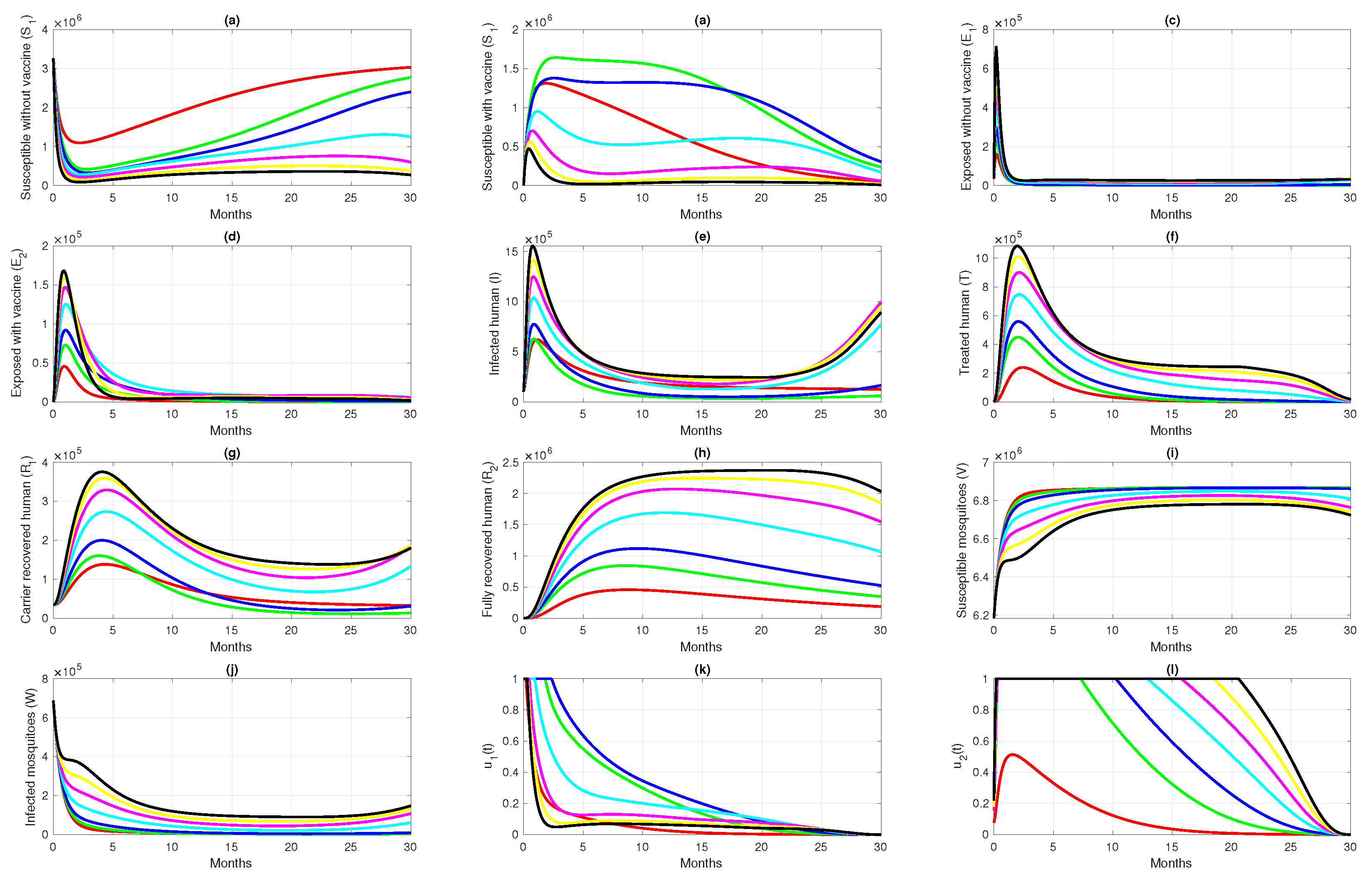
6.3. Different Initial Basic Reproduction Number

In this subsection, the optimal control simulation aims to see the effect of the initial value of the basic reproduction number when pre-erythrocytic intervention and transmission-blocking treatment is not yet implemented. In this case, the basic reproduction number of system (1) is given by (12).
For this simulation, we used parameter values as from Table 1, except that u 1 = 0 , u 2 = 0 , and also other parameters that related to the control parameters are zero as the base case (case 3 in Table 5). We run our simulation in seven different cases, and the differences are based on the value of β h 1 , β h 2 , and β v . Hence, we also have a different initial basic reproduction number R 0 , as shown in Table 5. It can be seen that the greater the value of R 0 , the higher the costs to reduce the high number of cases in the field. If we pay attention to Figure 13k,l, the higher the R 0 value, the longer the transmission-blocking treatment intervention should be given to its maximum value, and at the same time, the pre-erythrocytic intervention should be reduced in intensity to avoid high intervention costs. On the other hand, when R 0 is smaller, the pre-erythrocytic vaccine should be given for a longer period at its maximum level to avoid an increase in the number of malaria-infected individuals.

7. Conclusions

In this paper, we formulated and analyzed a deterministic compartmental model for malaria transmission. The model consists of eight compartments for humans and two compartments for mosquitoes. The malaria-free equilibrium is locally asymptotically stable if the basic reproduction number is less than unity. The basic reproduction number of our model presents the combination of infection paths in our transmission model, such as the bite of susceptible mosquitoes to the exposed human (with/without the vaccine), infected, treated, or carrier recovered individuals, or the bite of infected mosquitoes to susceptible humans (with/without vaccine).
Our model parameter values were estimated using incidence data from the Papua and West Papua provinces in Indonesia. We found that without implementing any type of intervention, the basic reproduction number of malaria in Papua and West Papua is greater than one, which suggests that a massive intervention should be made to reduce the spread of malaria. Our sensitivity analysis of the basic reproduction number shows that transmission-blocking is more sensitive to reducing the basic reproduction number compared to the pre-erythrocytic vaccine.
Several scenarios on the optimal control simulation were carried out based on the combination of interventions (first scenario), different initial conditions (second scenario), and the value of the basic reproduction number (third scenario). From the first simulation, in order to understand the most effective combination strategies, we found whether using both vaccine and treatment as a single or combined form of intervention will be more effective compared to other possible combinations. Our analysis shows that using both interventions is the most successful strategy in reducing the number of new infections. However, the number of averted infections with this strategy is only slightly different compared to that of implementing transmission-blocking treatment as a single form of intervention, but with a cheaper cost of implementation. On the other hand, the pre-erythrocytic vaccine is not recommended as a single form of intervention, as the result in reducing the number of infected individuals is not as significant as other strategies. From the second scenario, we concluded that more cost is needed to control malaria when the number of infected individuals is already high. For the last scenario, we run our simulation for various values of the basic reproduction number to indicate that the level of endemicity of malaria when vaccines and treatment are not yet implemented. Our results suggest the larger the basic reproduction number of an area, the larger the scale of the implementation of transmission-blocking treatment is needed to reduce the spread of malaria. Additionally, the pre-erythrocytic vaccine should be implemented at its maximum rate for a short period to minimize the intervention cost.

Author Contributions

Conceptualization, B.D.H., R.A.R. and D.A.; Formal analysis, B.D.H., R.A.R., C.W.C., S.H.A.K. and D.A.; Investigation, R.A.R., D.A. and S.H.A.K.; Methodology, B.D.H., R.A.R. and D.A.; Writing—original draft, B.D.H., R.A.R., C.W.C., S.H.A.K. and D.A. All authors have read and agreed to the published version of the manuscript.

Funding

This research was funded by Universitas Indonesia with PUTI Q2 research grant scheme, 2022 (ID: NKB-646/UN2.RST/HKP.05.00/2022).

Institutional Review Board Statement

Not applicable.

Informed Consent Statement

Not applicable.

Data Availability Statement

The data that been used in this research is from personal request to Papua and West Papua Provincial Health Office.

Acknowledgments

We thank anonymous reviewers for their valuable input and comments to help strengthen this paper.

Conflicts of Interest

The authors declare they do not have any competing interest.

References

  1. Vector-Borne Diseases. Available online: https://www.who.int/news-room/fact-sheets/detail/vector-borne-diseases (accessed on 20 January 2022).
  2. Malaria. Available online: https://www.who.int/health-topics/malaria#tab=tab_1 (accessed on 20 January 2022).
  3. CDC in Indonesia. Available online: https://www.cdc.gov/globalhealth/countries/indonesia/default.htm#malaria (accessed on 20 January 2022).
  4. About Malaria, Frequently Asked Questions. Available online: https://www.cdc.gov/malaria/about/faqs.html (accessed on 20 January 2022).
  5. Malaria. Available online: https://www.who.int/news-room/fact-sheets/detail/malaria (accessed on 20 January 2022).
  6. Larval Control and Other Vector Control Interventions. Available online: https://www.cdc.gov/malaria/malaria_worldwide/reduction/vector_control.html (accessed on 20 February 2022).
  7. Zheng, J.; Pan, H.; Gu, Y.; Zuo, X.; Ran, N.; Yuan, Y.; Zhang, C.; Wang, F. Prospects for Malaria Vaccines: Pre-erythrocytic Stages, Blood Stages, and Transmission-Blocking Stages. BioMed Res. Int. 2019, 2019, 9751471. [Google Scholar] [CrossRef]
  8. Duffy, P.E.; Gorres, J.P. Malaria vaccines since 2000: Progress, priorities, products. npj Vaccines 2020, 5, 48. [Google Scholar] [CrossRef]
  9. Ross, R. The Prevention of Malaria; John Murray: London, UK, 1911. [Google Scholar]
  10. Macdonald, G. The Epidemiology and Control of Malaria; Oxford University Press: Oxford, UK, 1957. [Google Scholar]
  11. Aron, J.L.; May, R.M. The population dynamics of malaria. In The Population Dynamics of Infectious Diseases: The Theory and Applications; Anderson, R.M., Ed.; Chapman and Hall: London, UK, 1982; pp. 139–179. [Google Scholar]
  12. Anderson, R.M.; May, R.M. Infectious Diseases of Humans: Dynamics and Control; Oxford University Press: Oxford, UK, 1991. [Google Scholar]
  13. Okosun, K.O.; Rachid, O.; Marcus, N. Optimal control strategies and cost-effectiveness analysis of a malaria model. Biosystems 2013, 111, 83–101. [Google Scholar] [CrossRef]
  14. Prosper, O.; Ruktanonchai, N.; Martcheva, M. Optimal vaccination and bed net maintenance for the control of malaria in a region with naturally acquired immunity. J. Theor. Biol. 2014, 352, 142–156. [Google Scholar] [CrossRef]
  15. White, M.T.; Verity, R.; Churcher, T.S.; Gnai, A.C. Vaccine approaches to malaria control and elimination: Insights from mathematical models. Vaccine 2015, 33, 7544–7550. [Google Scholar] [CrossRef] [Green Version]
  16. Woldegerima, W.A.; Ouifki, R.; Banasiak, J. Mathematical analysis of the impact of transmission-blocking drugs on the population dynamics of malaria. Appl. Math. Comput. 2021, 400, 126005. [Google Scholar] [CrossRef]
  17. Kuddus, M.A.; Rahman, A. Modelling and analysis of human–mosquito malaria transmission dynamics in Bangladesh. Math. Comput. Simul. 2022, 193, 123–138. [Google Scholar] [CrossRef]
  18. Aldila, D.; Angelina, M. Optimal control problem and backward bifurcation on malaria transmission with vector bias. Heliyon 2021, 7, e06824. [Google Scholar] [CrossRef]
  19. Beretta, E.; Capasso, V.; Garao, D.G. A mathematical model for malaria transmission with asymptomatic carriers and two age groups in the human population. Math. Biosci. 2018, 300, 87–101. [Google Scholar] [CrossRef]
  20. Forouzannia, F.; Gumel, A.B. Mathematical analysis of an age-structured model for malaria transmission dynamics. Math. Biosci. 2014, 247, 80–94. [Google Scholar] [CrossRef]
  21. Chen, H.; Wang, W.; Fu, R.; Luo, J. Global analysis of a mathematical model on malaria with competitive strains and immune responses. Appl. Math. Comput. 2015, 259, 132–152. [Google Scholar] [CrossRef]
  22. Fatmawati; Tasman, H.; Purwati, U.D.; Herdicho, F.F.; Chukwu, C.W. An optimal control problem of malaria model with seasonality effect using real data. Commun. Math. Biol. Neurosci. 2021, 2021, 66. [Google Scholar]
  23. Fatmawati; Herdicho, F.F.; Windarto; Chukwu, C.W.; Tasman, H. An optimal control of malaria transmission model with mosquito seasonal factor. Results Phys. 2021, 25, 104238. [Google Scholar] [CrossRef]
  24. Tchoumi, S.Y.; Diagne, M.L.; Rwezaura, H.; Tchuenche, J.M. Malaria and COVID-19 co-dynamics: A mathematical model and optimal control. Appl. Math. Model. 2021, 99, 294–327. [Google Scholar] [CrossRef]
  25. Ndii, M.Z.; Adi, Y.A. Understanding the effects of individual awareness and vector controls on malaria transmission dynamics using multiple optimal control. Chaos Solitons Fractals 2021, 153, 111476. [Google Scholar] [CrossRef]
  26. Handari, B.D.; Vitra, F.; Ahya, R.; Nadya S., T.; Aldila, D. Optimal control in a malaria model: Intervention of fumigation and bed nets. Adv. Differ. Equ. 2019, 2019, 497. [Google Scholar] [CrossRef]
  27. Okosun, K.O.; Ouifki, R.; Marcus, N. Optimal control analysis of a malaria disease transmission model that includes treatment and vaccination with waning immunity. Bio Syst. 2011, 106, 136–145. [Google Scholar] [CrossRef]
  28. Zhao, R.; Mohammed-Awel, J. A mathematical model studying mosquito-stage transmission-blocking vaccines. Math. Biosci. Eng. 2014, 11, 1229–1245. [Google Scholar] [CrossRef]
  29. Marques-da-Silva, C.; Peissig, K.; Kurup, S.P. Pre-Erythrocytic Vaccines against Malaria. Vaccine 2020, 8, 400. [Google Scholar] [CrossRef]
  30. First Malaria Vaccine Receives Positive Scientific Opinion from EMA. Available online: https://www.ema.europa.eu/en/news/first-malaria-vaccine-receives-positive-scientific-opinion-ema (accessed on 14 October 2020).
  31. Fischer, P.R. Malaria and Newborns. J. Trop. Pediatr. 2003, 49, 132–135. [Google Scholar] [CrossRef] [Green Version]
  32. Jumlah Penduduk Proyeksi (Jiwa) 2018–2020. Available online: https://papua.bps.go.id/indicator/12/277/1/jumlah-penduduk-proyeksi.html (accessed on 16 October 2021).
  33. Proyeksi Penduduk 2010–2020 (Jiwa) 2018–2020. Available online: https://papuabarat.bps.go.id/indicator/12/146/1/proyeksi-penduduk-2010-2020.html (accessed on 16 October 2021).
  34. Indikator Strategis Nasional. Available online: https://www.bps.go.id/QuickMap?id=0000000000 (accessed on 13 October 2021).
  35. About Malaria, Biology. Available online: https://www.cdc.gov/malaria/about/biology/index.html (accessed on 13 October 2021).
  36. Olotu, A.; Fegan, G.; Wambua, J.; Nyangweso, G.; Leach, A.; Lievens, M.; Kaslow, D.C.; Njuguna, P.; Marsh, K.; Bejon, P. Four-Year Efficacy of RTS,S/AS01E and Its Interaction with Malaria Exposure. N. Engl. J. Med. 2013, 368, 1111–1120. [Google Scholar] [CrossRef] [Green Version]
  37. Olotu, A.; Fegan, G.; Wambua, J.; Nyangweso, G.; Leach, A.; Lievens, M.; Kaslow, D.C.; Njuguna, P.; Marsh, K.; Bejon, P. Seven-Year Efficacy of RTS,S/AS01 Malaria Vaccine among Young African Children. N. Engl. J. Med. 2016, 374, 2519–2529. [Google Scholar] [CrossRef] [Green Version]
  38. Chitnis, N.; Hyman, J.M.; Cushing, J.M. Determining important parameters in the spread of malaria through the sensitivity analysis of a mathematical model. Bull. Math. Biol. 2008, 70, 1272–1296. [Google Scholar] [CrossRef]
  39. Lindblade, K.A.; Steinhardt, L.; Samuels, A.; Kachur, P.S.; Slutsker, L. The silent threat: Asymptomatic parasitemia and malaria transmission. Expert Rev. Anti-Infect. Ther. 2013, 11, 623–639. [Google Scholar] [CrossRef] [Green Version]
  40. Drakou, K.; Nikolaou, T.; Vasquez, M.; Petric, D.; Michaelakis, A.; Kapranas, A.; Papathedoulou, A.; Koliou, M. The effect of weather variables on mosquito activity: A snapshot of the main point of entry of Cyprus. Int. J. Environ. Res. Public Health 2020, 14, 1403. [Google Scholar] [CrossRef] [Green Version]
  41. Aldila, D. Optimal control for dengue eradication program under the media awareness effect. Int. J. Nonlinear Sci. Numer. Simul. 2021. [Google Scholar] [CrossRef]
  42. Aldila, D. Optimal control problem on COVID-19 disease transmission model considering medical mask, disinfectants and media campaign. E3S Web Conf. 2020, 202, 12009. [Google Scholar] [CrossRef]
  43. Hafidh, E.P.; Aulida, N.; Handari, B.D.; Aldila, D. Optimal control problem from tuberculosis and multidrug resistant tuberculosis transmission model. AIP Conf. Proc. 2018, 2023, 020223. [Google Scholar]
  44. Malaria: The Highest Cause of Death in the World. Available online: https://www.malaria.id/en/profile (accessed on 7 February 2022).
  45. St. Laurent, B.; Supratman, S.; Asih, P.B.S.; Bretz, D.; Mueller, J.; Miller, H.C.; Baharuddin, A.; Surya, A.; Ngai, M.; Laihad, F.; et al. Behaviour and molecular identification of Anopheles malaria vectors in Jayapura district, Papua province, Indonesia. Malar. J. 2016, 15, 192. [Google Scholar] [CrossRef] [Green Version]
  46. Mukandavire, Z.; Gumel, A.B.; Garira, W.; Tchuenche, J.M. Mathematical analysis of a model for HIV-malaria co-infection. Math. Biosci. Eng. 2009, 6, 333–362. [Google Scholar]
  47. Wadi, I.; Nath, M.; Anvikar, A.R.; Singh, P.; Sinha, A. Recent advances in transmission-blocking drugs for malaria elimination. Future Med. Chem. 2019, 11, 3047–3088. [Google Scholar] [CrossRef]
  48. Martcheva, M. An Introduction to Mathematical Epidemiology; Springer: New York, NY, USA, 2015. [Google Scholar]
  49. Roop-O, P.; Chinviriyasit, W.; Chinviriyasit, S. The effect of incidence function in backward bifurcation for malaria model with temporary immunity. Math. Biosci. 2015, 265, 47–64. [Google Scholar] [CrossRef]
  50. Chukwu, C.W.; Fatmawati. Modelling fractional-order dynamics of COVID-19 with environmental transmission and vaccination: A case study of Indonesia. AIMS Math. 2022, 7, 4416–4438. [Google Scholar] [CrossRef]
  51. Tsanou, B.; Kamgang, J.C.; Lubuma, J.M.-S.; Danga, D.E.H. Modeling pyrethroids repellency and its role on the bifurcation analysis for a bed net malaria model. Chaos Solitons Fractals 2020, 136, 109809. [Google Scholar] [CrossRef]
  52. Diekmann, O.; Heesterbeek, J.A.; Roberts, M.G. The construction of next-generation matrices for compartmental epidemic models. J. R. Soc. Interface 2010, 7, 873–885. [Google Scholar] [CrossRef] [Green Version]
  53. Marino, S.; Hogue, I.B.; Tay, C.J.; Kirschner, D.E. A methodology for performing global uncertainty and sensitivity analysis in systems biology. J. Theor. Biol. 2008, 254, 178–196. [Google Scholar] [CrossRef] [Green Version]
  54. Chukwu, C.W.; Nyabadza, F. Mathematical Modeling of Listeriosis incorporating effects of awareness programs. Math. Mod. Comput. Simul. 2021, 13, 723–741. [Google Scholar] [CrossRef]
  55. Cesari, L. Optimization–Theory and Applications, Problems with Ordinary Differential Equations, Applications of Mathematics; Springer: New York, NY, USA, 1983. [Google Scholar]
  56. Fleming, W.H.; Rishel, R.W. Deterministic and Stochastic Optimal Control; Springer: New York, NY, USA, 1975. [Google Scholar]
  57. Lukes, D.L. Differential Equations: Classical to Controlled; Academic Press: New York, NY, USA, 1982. [Google Scholar]
  58. Pontryagin, L.S.; Boltyanskii, V.G.; Gamkrelize, R.V.; Mishchenko, E.F. The Mathematical Theory of Optimal Processes; Interscience Publishers (Division of John Wiley and Sons, Inc.): New York, NY, USA, 1962. [Google Scholar]
  59. Lenhart, S.; Workman, J.T. Optimal Control Applied to Biological Models, 1st ed.; Chapman and Hall/CRC: New York, NY, USA, 2007. [Google Scholar]
Figure 1. Transmission diagram of model (1).
Vaccines 10 01174 g001
Figure 2. Estimation result on fitting the accumulated cases in Papua with c ( t ) in Equation (3). The best-fit initial conditions for S 1 , E 1 , I , T , R 1 , R 2 , V , W are 3,435,430, 2000, 2000, 2000, 1000, 21, 6,870,860, 3000, respectively.
Vaccines 10 01174 g002
Figure 3. Estimation result of fitting the accumulated cases in West Papua with c ( t ) in Equation (3). The best-fit initial conditions for S 1 , E 1 , I , T , R 1 , R 2 , V , W are 974,300, 400, 400, 51, 21, 125, 1,789,099, 202, respectively.
Vaccines 10 01174 g003
Figure 4. Illustration for the existence of malaria-endemic equilibrium point.
Vaccines 10 01174 g004
Figure 5. Tornado plot showing the PRCC values for the model parameters in R 0 .
Vaccines 10 01174 g005
Figure 6. Local sensitivity analysis with full–normalization technique of all variables with respect to all parameters (a) and without δ 1 (b). We use incidence data from Papua and the following initial conditions: S 1 ( 0 ) = 3,208,839 , S 2 ( 0 ) = 0 , E 1 ( 0 ) = 2000 , E 2 ( 0 ) = 0 , I ( 0 ) = 2000 , T ( 0 ) = 1000 , R 1 ( 0 ) = 1000 , R 2 ( 0 ) = 317 , V ( 0 ) = 6,664,102 , W ( 0 ) = 2781 to run the simulation.
Vaccines 10 01174 g006
Figure 7. Local sensitivity analysis with full–normalization technique of all variables with respect to all parameters (a) and without δ 1 (b). We use incidence data from West-Papua and the following initial conditions: S 1 ( 0 ) = 918,167 , S 2 ( 0 ) = 0 , E 1 ( 0 ) = 399 , E 2 ( 0 ) = 0 , I ( 0 ) = 242 , T ( 0 ) = 51 , R 1 ( 0 ) = 22 , R 2 ( 0 ) = 88 , V ( 0 ) = 1,915,967 , W ( 0 ) = 641 to run the simulation.
Vaccines 10 01174 g007
Figure 8. Dynamics of human (ah), mosquitoes (i,j), and controls (k,l) under the scenario of pre-erythrocytic vaccine intervention only applies. Blue and red curve represents implementation strategies with and without controls.
Vaccines 10 01174 g008
Figure 9. Dynamics of human (ah), mosquitoes (i,j), and controls (k,l) under the scenario of transmission-blocking treatment intervention only applies. Blue and red curve represents implementation strategies with and without controls.
Vaccines 10 01174 g009
Figure 10. Dynamics of human (ah), mosquitoes (i,j), and controls (k,l) under the scenario of both intervention applies. Red and blue curve present a condition of without and with implementation of control.
Vaccines 10 01174 g010
Figure 11. Dynamics of total susceptible human (a) total of infected human (b) for four different strategies (no intervention (red), u 1 and u 2 (blue), u 1 only (black), and u 2 only (magenta)).
Vaccines 10 01174 g011
Figure 12. Dynamics of human (ah), mosquitoes (i,j), and controls (k,l) under the scenario of both intervention applies, but with a higher number of infected individuals at time t = 0 . Red and blue curve present a condition of without and with implementation of control.
Vaccines 10 01174 g012
Figure 13. Time series dynamics for; humans (ah), mosquitoes (i,j), and controls (k,l), but different initial R 0 when no control applied. The color in the legend are explained in Table 5.
Vaccines 10 01174 g013
Table 1. The parameters of malaria model in (1). Some parameter values are taken from parameter estimation results in Section 2.2 and the rest are from assumptions.
SymbolsBiological DefinitionsPapuaWest PapuaSources
Π h Natural birth rate of humans 3 , 435 , 430 71.5 × 12 981 , 822 71.5 × 12 [32,33,34]
Π v Natural birth rate of mosquitos 2 × 3 , 435 , 430 21 30 2 × 981 , 822 21 30 [32,33,35]
bThe average number of mosquitoes bite per unit time 9.07523 5.94285 estimated
β h 1 ¯ The successful transmission rate of susceptible humans per bite 0.89999 0.87753 estimated
β h 2 ¯ The successful transmission rate of susceptible humans who receive pre-erythrocytic vaccine per bite 0.42299 0.41244 estimated
β h 1 = b β h 1 ¯ N Average infection rate to humans per unit time per mosquito 2.37749 × 10 6 5.31162 × 10 6 estimated
β h 2 = b β h 2 ¯ N Average infection rate to humans who receive pre-erythrocytic vaccine per unit time per mosquito 1.11742 × 10 6 2.49646 × 10 6 estimated
β v ¯ Average of successful transmission rate of susceptible mosquitos per bite 0.00572 0.01054 estimated
β v = b β v ¯ N Average infection rate to mosquitos per unit time per human 1.51190 × 10 8 6.38376 × 10 8 estimated
κ Waning rate of temporal immunity from recovered carriers 0.33333 0.33333 estimated
ϑ Waning rate of temporal immunity from fully recovered class 0.05555 0.05555 estimated
u 1 Vaccination rate with pre-erythrocytic vaccine 0.001 0.001 assumption
u 2 Rate of treatment with transmission-blocking drugs 0.499999 0.499997 estimated
1 ξ pre-erythrocytic vaccine efficacy level 0.53 0.53 [36]
α Waning rate of vaccine efficacy 1 6 1 6 [37]
δ 1 Progression rate from exposed without vaccine class 6.08333 6.08333 estimated
δ 2 Progression rate from exposed with vaccine class22[36,38]
γ 1 Natural recovery rate of infected humans by immune response 0.19999 0.19999 estimated
γ 2 1 Duration of treatment with transmission-blocking drugs 1 1.08631 1 1.08631 estimated
pProportion of people in treatment who managed to get protection 0.59999 0.59964 estimated
qProportion of people in treatment who fail to receive protection and then recover naturally 0.29999 0.29994 estimated
1 p q Proportion of people in treatment who fail to receive protection and then return to the infected class 0.100000004 0.10040 estimated
ζ e 1 Correction factor for infection rate in mosquitoes by exposed humans 0.04999 0.04999 estimated
ζ e 2 Correction factor for infection rate in mosquitoes by exposed humans with vaccine 0.03999 0.03999 assumption
ζ r Correction factor for infection rate in mosquitoes by recovered humans but carrier 0.06 0.06 estimated
ζ t Correction factor for infection rate in mosquitoes by humans in treatment 0.08 0.08 estimated
μ h Natural death rate of humans 1 71.5 × 12 1 71.5 × 12 [34]
μ v Natural death rate of mosquitos 30 21 30 21 [35]
Table 2. Lower and upper bound of parameters that will be estimated.
ParametersInterval ValuesSources
Π h 3 , 435 , 430 71.5 × 12 or 981 , 822 71.5 × 12 [32,33,34]
Π v 2 × 3 , 435 , 430 × 30 21 or 2 × 981 , 822 × 30 21 [32,33,35]
b 3.012 , 17.4 [27]
β h 1 ¯ 0.03 , 0.9 [16,27]
β h 2 ¯ 0.47 × 0.03 , 0.47 × 0.9 [16,27,36]
β h 1 = b β h 1 ¯ N 2.63 × 10 8 , 4.22 × 10 6 or 9.20 × 10 8 , 1.47 × 10 5 [27,32,33]
β h 2 = b β h 2 ¯ N 1.23 × 10 8 , 1.98 × 10 6 or 4.32 × 10 8 , 6.94 × 10 6 [27,32,33,36]
β v ¯ 0.00572 , 0.09 [27]
β v = b β v ¯ N 5.01 × 10 9 , 4.55 × 10 7 or 1.75 × 10 8 , 1.59 × 10 6 [27,32,33]
κ 1 12 , 1 3 [38]
ϑ 1 18 , 1 3 [38]
u 1 0 , 1 varied
u 2 0 , 1 varied
1 ξ 0.53 [36]
α 1 4 × 12 , 1 4 [37]
δ 1 2.02778 , 6.08334 [38]
δ 2 0.9530566 , 2.8591698 [36,38]
γ 1 1 12 , 1 5 [46]
γ 2 0.7242071429 , 1.086310714 [47]
p 0 , 1 varied
q 0 , 1 varied
1 p q 0 , 1 varied
ζ e 1 0.00001 , 1 [16]
ζ e 2 0 , 1 varied
ζ r 0.005 , 1 [16]
ζ t 0.02 , 1 [16]
μ h 1 71.5 × 12 [34]
μ v 30 21 [35]
Table 3. Parameter values to show existence of E .
ParameterValueParameterValue
κ 0.333333327466586 γ 1 0.199999993947735
ϑ 0.0555555854358188 γ 2 1.08631070229205
α 1 6 β v 1.51190029406934 × 10 8
β h 1 2.37749246426963 × 10 6 ζ e 1 0.0499997440960968
u 1 0.001 ζ e 2 0.0399997440960968
β h 2 1.11742145820672 × 10 6 ζ t 0.080000001876738
δ 1 6.08333998105411 ζ r 0.060000000761188
δ 2 2 μ h 1.165501166 × 10 3
p 0.599999998192909 Π h 4003.99766899767
q 0.299999997668467 μ v 1.428571429
u 2 0.499999999825239 Π v 9,815,514.28571429
Table 4. PRCC parameter values and p-values for the global sensitivity analysis against R 0 .
ParameterPRCC Valuesp-ValuesSignificant?
Π h 0.271036046 0TRUE
β h 1 0.631568463 0TRUE
μ h 0.656060428 0TRUE
μ v 0.856948705 0TRUE
β v 0.643359162 0TRUE
ξ e 1 0.038340724 2.282 × 10 1 FALSE
Π v 0.276430743 0TRUE
δ 1 0.003574822 9.106 × 10 1 FALSE
γ 1 0.162743705 2.486 × 10 7 TRUE
κ 0.079425150 1.240 × 10 2 FALSE
ξ r 0.183579610 5.425 × 10 9 TRUE
Table 5. Numerical results for various initial value of the non-controlled basic reproduction number.
CaseScenario for β h 1 , β h 2 and β v R 0 Inverted CaseCostColour
1Reduced 50% from case 31.00552,787 7.038 × 10 11 Red
2Reduced 25% from case 31.508129,702 1.101 × 10 12 Green
3As in Table 1 for Papua data2.011170,680 1.334 × 10 12 Blue
4Increased 50% from case 33.016185,168 1.857 × 10 12 Cyan
5Increased 100% from case 34.022183,584 2.67 × 10 12 Magenta
6Increased 150% from case 35.027184,294 3.573 × 10 12 Yellow
7Increased 200% from case 36.033185,505 4.562 × 10 12 Black
Publisher’s Note: MDPI stays neutral with regard to jurisdictional claims in published maps and institutional affiliations.

